
94% of researchers rate our articles as excellent or good
Learn more about the work of our research integrity team to safeguard the quality of each article we publish.
Find out more
ORIGINAL RESEARCH article
Front. Mar. Sci., 28 November 2022
Sec. Marine Biology
Volume 9 - 2022 | https://doi.org/10.3389/fmars.2022.1049056
This article is part of the Research TopicSharing Technical Knowledge to Understand the Distribution Patterns and Migration History of Marine OrganismsView all 11 articles
 Jun Matsubayashi1*
 Katsuya Kimura1
 Naohiko Ohkouchi2
 Nanako O. Ogawa2
 Naoto F. Ishikawa2Yoshito Chikaraishi3Yuichi Tsuda1Hiroshi Minami1
Tracking migration of highly migratory marine fish using isotope analysis (iso-logging) has become a promising tool in recent years. However, application of this method is often hampered by the lack of essential information such as spatial variations in isotope ratios across habitats (isoscapes) and ontogenetic shifts of isotope ratios of target animals. Here, we test the utility of geostatistical analysis to generate isoscapes of δ13C and δ15N in the western Pacific and estimate the ontogenetic shifts in δ13C and δ15N values of a target species. We first measured δ13C and δ15N in the white muscle of juvenile (n = 210) and adult (n = 884) skipjack tuna Katsuwonus pelamis sampled across the northwest Pacific. Next we fitted a geostatistical model to account for the observed spatial variations in δ13C and δ15N of skipjack by fork length and other environmental variables with spatial random effects. We then used the best-fit models to predict the isoscapes of δ13C and δ15N in 2021. Furthermore, we measured δ15N of amino acids (δ15NAAs) of skipjack (n = 5) to determine whether the observed spatial variation of isotope ratios resulted from baseline shifts or differences in trophic position. The geostatistical model reasonably estimated both isoscapes and ontogenetic shifts from isotope ratios of skipjack, and the isoscapes showed that δ13C and δ15N can clearly distinguish the latitudinal migration of skipjack in the western Pacific. The δ15NAAs supported the results of the geostatistical model, that is, observed variations in skipjack δ15N were largely derived from a baseline shift rather than regional differences in trophic position. Thus, we showed that geostatistical analysis can provide essential basic information required for iso-logging without compound-specific isotope analysis.
Shared fish stocks, namely fish resources with high migration ability that cross exclusive economic zone (EEZ) boundaries, are more prone to overexploitation than other stocks (e.g. McWhinnie, 2009; Kraska et al., 2015; Popova et al., 2019). Therefore, cooperative stock management among stakeholders is a necessary prerequisite for achieving sustainable fisheries of these species (e.g. Caddy, 1997; Miller and Munro, 2004). Appropriate understanding of migration routes and their individual and temporal variation is crucial for better cooperative management of shared fish stocks. Knowledge of a migration route is also essential for determining which countries share fishery resources from the same stock, as well as for assessing the effect of changes in the migration routes on the stock and fishing conditions in each country (Miller and Munro, 2004; Vatsov, 2016). Recently developed models (e.g. Carvalho et al., 2015; Sippel et al., 2015) can make use of migration data for stock assessment, thus demonstrating the benefits of understanding the migration routes of these fish.
In fishery science, one of the main approaches for studying fish migration is dynamic tracking using electronic technologies such as telemetry, radio, and computer networks (e.g. Priede et al., 1988; Thorstad et al., 2013). Although these methods have excellent spatial and temporal resolution, there are several intrinsic drawbacks, such as the high cost of bio-logging equipment (Hebblewhite and Haydon, 2010; Graves and Horodysky, 2015), the large effort required for capturing and tagging the fish, and body-size limitations for tagged fish: conventionally, the recommended tag weight is less than 3% of the fish body mass (e.g. Winter, 1983; Jepsen et al., 2002; Cooke et al., 2011). Stock assessment models are generally based on population-level data, but bio-logging methods only yield individual-level inferences, making them difficult to incorporate into overall stock condition assessments. In addition, equipment attached to a target fish can change its behavior, potentially resulting in biased migration data, although the effect is highly context-dependent and species-specific (Jepsen et al., 2015).
To overcome these drawbacks of bio-logging and make use of migration data for stock assessment of shared fish stocks, other approaches with lower cost and less effort are warranted. Recently, migration tracking techniques using isotope analysis of incremental-growth tissues such as otoliths, eye lenses, and vertebral bones (Matsubayashi et al., 2017; Sakamoto et al., 2019; Matsubayashi et al., 2020; Vecchio and Peebles, 2020) have proven promising for inferring the migration routes of individual fish. The isotopic composition of local environment and an animal’s tissue can be used as a natural tag to track its movements through isotopically distinct habitats (Graham et al., 2010), and we call this technique “iso-logging”. The major advantages of iso-logging over bio-logging are lower cost and effort, longer period of tracking (Vecchio and Peebles, 2020), and no influence on the behavior of target fish before death, although the temporal resolution and accuracy of estimated ranges are not equal to those from bio-logging.
In the case of marine fish, the 18O:16O ratio (δ18O) in otoliths is the most frequently used isotope ratio for iso-logging (e.g. Trueman et al., 2012; Hsieh et al., 2019; Sakamoto et al., 2019). δ18O can be retrospectively measured from otoliths and reflects the ambient temperature experienced by the fish. However, δ18O is not effective for iso-logging of fish that 1) migrate in oceans with similar thermal gradients, 2) have a stable body temperature, like tuna (Thunnus spp.; Carey and Teal, 1969), or 3) often dive deep, crossing the thermocline. Skipjack tuna Katsuwonus pelamis comprises one of the most commercially important shared fish stocks inhabiting warm and temperate waters. Skipjack in western Pacific populations prefer sea-surface temperatures ranging from 20.5 to 26.0°C (Mugo et al., 2010) and can maintain its body temperature higher than that of ambient water (Barrett and Hester, 1964; Stevens et al., 1974), which hampers the use of otolith δ18O for migration tracking. For this reason, it is necessary to test the applicability of other isotope ratios for tracking skipjack migration. Recent studies have suggested that stable carbon and nitrogen isotope ratios (δ13C and δ15N) can be excellent indicators for the migration histories of marine animals in some areas (Trueman et al., 2017; Matsubayashi et al., 2020), and these isotopes may be also applicable for tracking skipjack in the western Pacific (Coletto et al., 2021).
To use δ13C and δ15N for iso-logging of marine fish, at least three types of information are required: 1) the isoscapes across the habitat, 2) any ontogenetic shifts of isotope ratios of target fish, and 3) isotopic offsets between isoscapes and target fish. Unfortunately, it is generally difficult to obtain all of this information for δ13C and δ15N. The generation of isoscapes requires thorough field sampling of proxy organisms with low swimming ability (Trueman et al., 2017; Matsubayashi et al., 2020). Understanding isotopic offsets between isoscape and target animal requires feeding experiments over several months (e.g. Matsubayashi et al., 2019; Canseco et al., 2021). Furthermore, in the case of highly migratory piscivorous species, understanding the ontogenetic shifts of δ13C and δ15N is particularly difficult because isoscapes and ontogenetic dietary shifts have mutual interactions. To overcome these difficulties in iso-logging, we conceived of using a geostatistical model to simultaneously estimate isoscapes and ontogenetic shifts of isotope ratios using the fish targeted for migration tracking as a proxy organism for isoscapes. With this approach, isotopic offsets between isoscapes and target fish can be ignored. Although such modeling was technically difficult up until a few years ago, recent advances in geostatistical analysis (e.g. Rue et al., 2009; Thorson, 2019; Anderson et al., 2022) allow us to account for these factors in a single model with a user-friendly interface.
Here, we test the utility of geostatistical analysis for generating isoscapes using δ13C and δ15N of skipjack in the western Pacific, considering ontogenetic shifts in isotope ratios of this species. In this region, skipjack is mainly distributed from 20°S to 40°N and from 110°E to 180°E (Bartoo, 1987; Kiyofuji and Ochi, 2016), and some individuals exhibit dynamic northward migration from the subtropics into waters off the Pacific coast of Japan (Kiyofuji et al., 2019a). The water temperature range preferred by skipjack is from 18.8°C to 28.1°C and the 18.0 isotherm is the lowest thermal limit of skipjack tuna distribution (Kiyofuji et al., 2019a). We sampled the muscle tissue of skipjack of various body sizes and determined the δ13C and δ15N values of bulk tissue (δ13CBulk and δ15NBulk). We then applied a geostatistical model to account for variations in the δ13C and δ15N of skipjack muscle with fork length, several environmental variables, and a spatial random field. Furthermore, we performed compound-specific nitrogen isotope analysis of amino acids (δ15NAAs) for five samples with different δ15NBulk values to evaluate whether the differences in bulk values resulted from a baseline shift in isotope ratios or from trophic differences (see Matsubayashi et al., 2020). On the basis of these data, we discuss the applicability of δ13CBulk and δ15NBulk for assessing the migration of skipjack in the western Pacific.
Samples of juvenile skipjack (n = 210) were collected during 1995–2019 from multiple sampling stations in the western Pacific by mid-water trawl (mesh size: 16mm) during several research cruises of the Fisheries Resources Institute, Japan Fisheries Research and Education Agency. Juvenile fish from the EEZs of countries other than Japan were collected under formal agreement with each country. The 20 cm fork length is the threshold that distinguishes juvenile from adults, and it takes about 3 months for skipjack to reach this length (Kiyofuji et al., 2019b). Dorsal white muscle sampled from juvenile fish was rinsed in distilled water for at least six hours, because the samples were preserved in ethanol, and then the samples were freeze-dried. Most samples of adult skipjack (n = 884) were purchased from commercial fisheries, and some were caught by research vessel surveys. None of them were from the EEZ of countries other than Japan (Figure 1). Dorsal white muscle was sampled from each fish and kept frozen until isotopic analysis. The sampling stations for skipjack ranged from 5.0°S to 40.9°N and from 123.0°E to 164.9°E (Figure 1). The muscle samples were ground into fine powder and defatted using a methanol:chloroform mixture (1:2, v:v) and then used for bulk and compound-specific isotopic analyses.
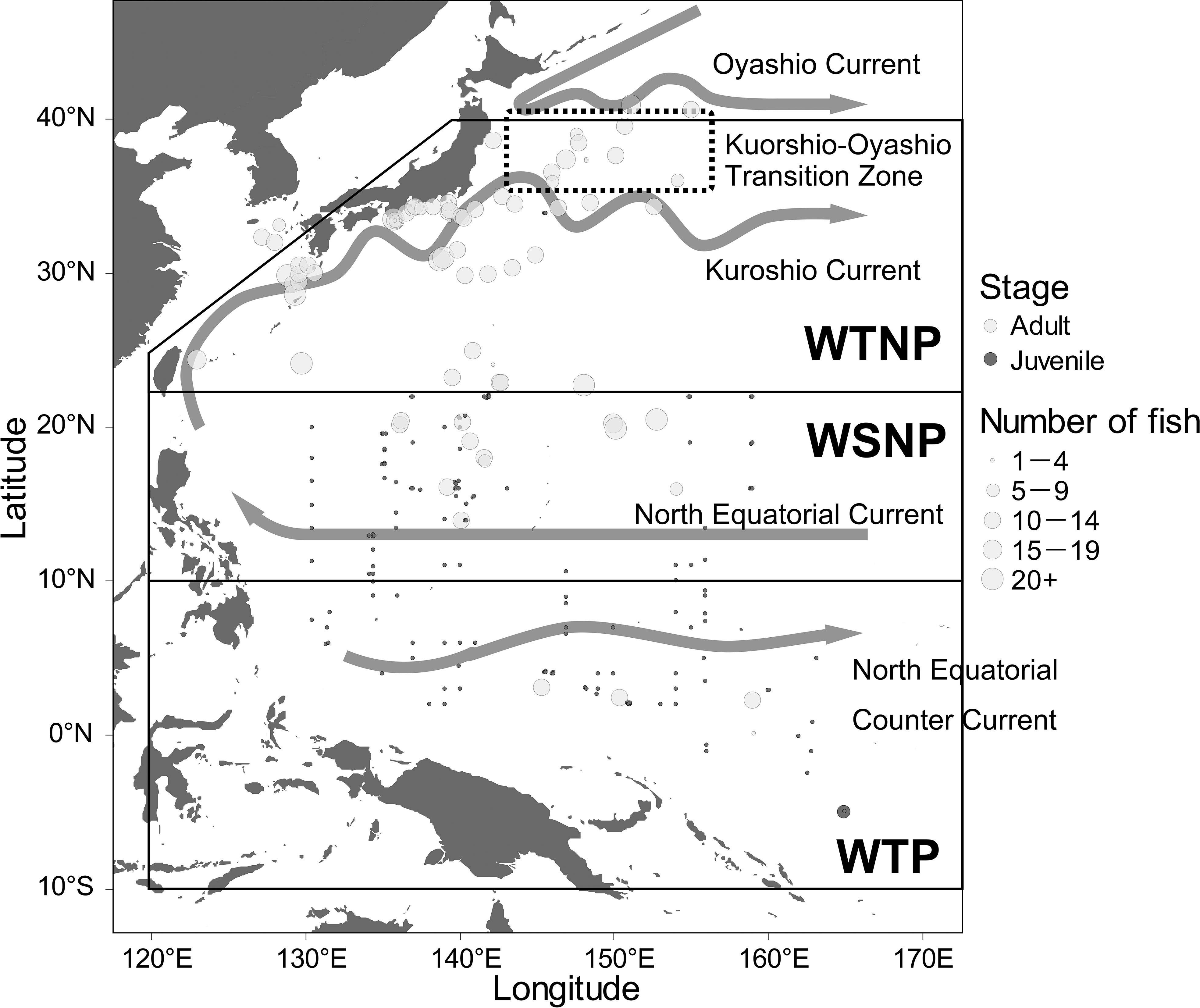
Figure 1 Sampling points and sample sizes of juvenile and adult skipjack tuna (Katsuwonus pelamis), boundaries of the western tropical Pacific (WTP), western subtropical North Pacific (WSNP), western temperate North Pacific (WTNP), and schematic diagram of the major currents in the western Pacific Ocean. The Kuroshio-Oyashio Transition Zone is known to have high net primary productivity (Nishikawa et al., 2020).
The δ13CBulk and δ15NBulk values were measured using continuous-flow elemental analyzer (EA)/isotope-ratio mass spectrometry (IRMS) systems. Stable isotope ratios are expressed in conventional δ notation in accordance with the international standard scale, based on the following equation:
where X is 13C or 15N, Rsample is the 13C:12C or 15N:14N ratio of the sample, and Rstandard is that of Vienna Pee Dee Belemnite (VPDB) or atmospheric nitrogen (AIR), respectively. Elemental concentrations and isotope ratios of carbon and nitrogen were calibrated against those of alanine, glycine, and histidine laboratory standards, which are traceable back to international standards. The analytical errors (SDs) of δ13C and δ15N were smaller than 0.18‰ and 0.16‰, respectively.
The δ13CBulk and δ15NBulk values allow the study area to be isotopically divided into at least three regions: the western tropical Pacific (WTP), western subtropical North Pacific (WSNP), and western temperate North Pacific (WTNP). We chose a total of five skipjack samples representing the δ13CBulk and δ15NBulk values in each region for δ15NAAs analysis. Samples for δ15NAAs were prepared using a method based on the amino-acid derivatization procedures described in Chikaraishi et al. (2015) as follows. Samples were initially hydrolyzed with 12 M HCl at 110°C overnight (>12 h) and then washed with n-hexane:dichloromethane (3:2, v:v) to remove any hydrophobic constituents. After hydrolysis, samples were derivatized using thionyl chloride:2-propanol (1:4, v:v) at 110°C for 2 h and then pivaloyl chloride:dichloromethane (1:4, v:v) at 110°C for 2 h. The amino-acid derivatives were then extracted with n-hexane:dichloromethane (3:2, v:v). The δ15N value of each amino acid was determined by gas chromatography/combustion/isotope-ratio mass spectrometry (GC/C/IRMS) using a 6890N GC instrument (Agilent Technologies, Palo Alto, CA, USA) coupled to a Delta plus XP IRMS via GC-combustion III interface (Thermo Finnigan, Bremen, Germany) at the Japan Agency for Marine-Earth Science and Technology. Reference mixtures of nine amino acids (alanine, glycine, leucine, norleucine, aspartic acid, methionine, glutamic acid, phenylalanine, and hydroxyproline) with known δ15N values (ranging from −26.4‰ to +45.6‰; Indiana University, Bloomington, IN, USA, and SI Science Co., Sugito-machi, Japan) were analyzed every four to six sample runs. The average SD of the standards was 0.7‰ (n = 16).
The trophic positions (TPs) of the fish sampled for δ15NAAs (n = 5) were estimated from differences between the δ15N values of glutamic acid and phenylalanine as follows (Chikaraishi et al., 2009):
where δ15NGlu is the δ15N of glutamic acid, δ15NPhe is the δ15N of phenylalanine, β is the difference between δ15NGlu and δ15NPhe in primary producers, and TDFGlu-Phe is the trophic discrimination factor for δ15N of glutamic acid relative to phenylalanine. We used a value of 3.4 for β and 7.6‰ for TDFGlu-Phe (Chikaraishi et al., 2009).
Data for the following environmental variables in the euphotic zone (depth < 100 m) of the western Pacific were obtained from Copernicus Marine Environment Monitoring Service (CMEMS, https://marine.copernicus.eu/): potential temperature, salinity, concentrations of chlorophyll a, dissolved oxygen, nitrate, phosphate, and iron, and surface partial pressure of carbon dioxide (spCO2). These data have at most four dimensions: latitude, longitude, date (year and month), and depth. Among these, latitude and longitude were set to the same as the skipjack sampling points; however, it was necessary to assume an interval for data aggregation of date and depth prior to allocating the environmental variables for each data point.
To determine the aggregation interval for the environmental information for each data point, we estimated the isotopic turnover rate (i.e., the rate at which the elements comprising a tissue are replaced) of muscle for adult and juvenile skipjack. Although there are no empirical studies estimating species-specific turnover times for skipjack, Coletto et al. (2021) suggested that adult skipjack has a shorter turnover time than Thunnus species, considering the faster growth rates of this species, and assumed a turnover time similar to those estimated for juvenile yellowfin tuna (around 2–4 months; Graham et al., 2007). For this reason, we used the average values of the environmental variables at each sampling point over the four months leading up to and including the sampled month for adult fish with fork length greater than 200 mm. Because juvenile fish with fork length<200 mm seem to have shorter turnover times than adult fish, given their higher growth rate (Hoyle et al., 2011), we used monthly mean values of environmental variables at each sampling point for the sampled year and month for juvenile skipjack.
As the representative depth for aggregating the environmental variables, we selected the depth at which the concentration of phytoplankton was highest by using data for phytoplankton concentration from CMEMS, assuming that δ13C and δ15N of phytoplankton at that depth were the main influences on the values in skipjack muscle. We then extracted and allocated the environmental variables at the location, period and depth corresponding to each data point (Supplementary Table 1).
To estimate spatial distributions of δ13CBulk and δ15NBulk values in the western Pacific, we used the R package “sdmTMB” ver. 0.0.26.9001 (Anderson et al., 2022), which accounts for independent region-specific noise via the stochastic partial differential equations (SPDE) approach. In sdmTMB, the spatial random effect is assumed to form continuous Gaussian Markov random fields (GMRF) and is approximated by creating a Delaunay triangularized mesh over the study area (Lindgren et al., 2011). sdmTMB makes use of the integrated nested Laplace approximation (INLA; Rue et al., 2009) to create the triangularized meshes. We set the number of nodes to 200 and determined the optimal cutoff value for the number of nodes via the “cutoff_search” option in sdmTMB (Anderson et al., 2022). Meshes on land were transformed into barrier meshes (meshes with correlation barriers) using the “add_barrier_mesh” function of sdmTMB (Anderson et al., 2022).
To maximize the prediction ability of the model, we implemented thin plate regression splines (Wood, 2003) for all covariates. We used smoothers with specified basis dimensions (k values), which were 3 for fork length and 5 for the other covariates. A smaller basis dimension (k = 3) was assumed for fork length because the relationships between fork length and δ13CBulk and δ15NBulk are expected to be either positive linear or positive asymptotic relationships (Fry and Sherr, 1984; Minagawa and Wada, 1984). The relationships between δ13CBulk or δ15NBulk and the other parameters were unknown, hence we assigned these a larger basis dimension (k = 5). We did not implement temporal random effects because there is a large bias in the year the samples were taken. The response variables were modelled using the Gaussian family with identity link function.
From this, the model can be specified as: yi = α0 + Xiβ + Wi where yi is the δ13CBulk or δ15NBulk value of skipjack muscle at sampling location i (i = 1, …, n; n = 1094), α0 is the intercept, β is the vector of regression parameters, Xi is the matrix of the explanatory covariates (fork length and environmental variables) at location i, and Wi represents the spatially structured random effect at location i. We searched for the best combinations of the covariates (Xi) for prediction of δ13CBulk and δ15NBulk values of skipjack muscle by model selection based on the Akaike information criterion (AIC). We tested three options for each covariate—the variable with smoothing, the variable without smoothing, and without the variable at all—and then calculated the AIC for models with all combinations of these three options for nine covariates. Due to computational time limitations for model selection, we could not incorporate additional explanatory variables such as the effect of season. St John Glew et al. (2021) incorporated the effect of season as explanatory variables, which improved the model predictions. However, we believe that seasonal effects are not an important variable in our model, because the CMEMS environmental data are themselves highly seasonally variable, and their effects are incorporated into the model with smoothing splines. Finally, models with the smallest AIC were chosen as best-fit models for the prediction of δ13CBulk and δ15NBulk values of skipjack muscle.
For the best fit models, sanity checks on the items listed below were performed by the “sanity” function of sdmTMB; the non-linear minimizer suggests successful convergence, the Hessian matrix is positive definite, no extreme or very small eigen values are detected, no gradients with respect to fixed effects are greater than 0.001, no fixed-effect standard errors are not applicable (N/A), no fixed-effect standard errors look unreasonably large, no sigma parameters are less than 0.001, and the range parameter does not look unreasonably large. All statistical analysis was conducted using R (R Core Team, 2021).
To generate isoscapes of δ13C and δ15N in the western Pacific, we obtained monthly mean values of the environmental variables within the triangularized meshes of sdmTMB from January to December 2021 from CMEMS. The environmental variables were then fitted with the best-fit models of δ13C and δ15N to generate isoscapes for 2021, while fork length was set to 0. The uncertainties (standard deviations) of spatial prediction were estimated via simulation from the fitted model (n = 500). Predictions with uncertainty >2 for δ15N and >1 for δ13C were excluded from the isoscapes to avoid excessive extrapolation.
The fork length of skipjack sampled ranged from 11 to 834 mm (384 ± 186 mm), and that of juveniles and adults were from 11 to 170 mm (36 ± 26 mm) and from 25 to 83 mm (466 ± 85 mm), respectively. Juveniles were distributed from 130.4°E to 164.9°E (mean 146.0°E) and from 5.0°S to 33.9°N (10.0°N) Adults were found from 123.0°E to 159.0°E (140.1°E) and from 2.3°S to 40.9°N (28.8°N) (Figure 1). The sample sizes at each sampling station were generally small for juvenile fish (1.3 ± 0.7) but large for adult fish (11.5 ± 7.7).
The observed δ13CBulk and δ15NBulk values of skipjack ranged from –20.0‰ to –15.7‰ (mean ± SD, –17.8‰ ± 0.8‰) and from 3.1‰ to 18.9‰ (9.7‰ ± 2.4‰), respectively. Skipjack in the WTP had high δ15NBulk values and those in the WSNP and WTNP had low and intermediate values, respectively (Figure 2). The spatial variation in δ13CBulk of skipjack muscle is characterized by lower values in the WTNP than in the WSNP and WTP (Figure 2).
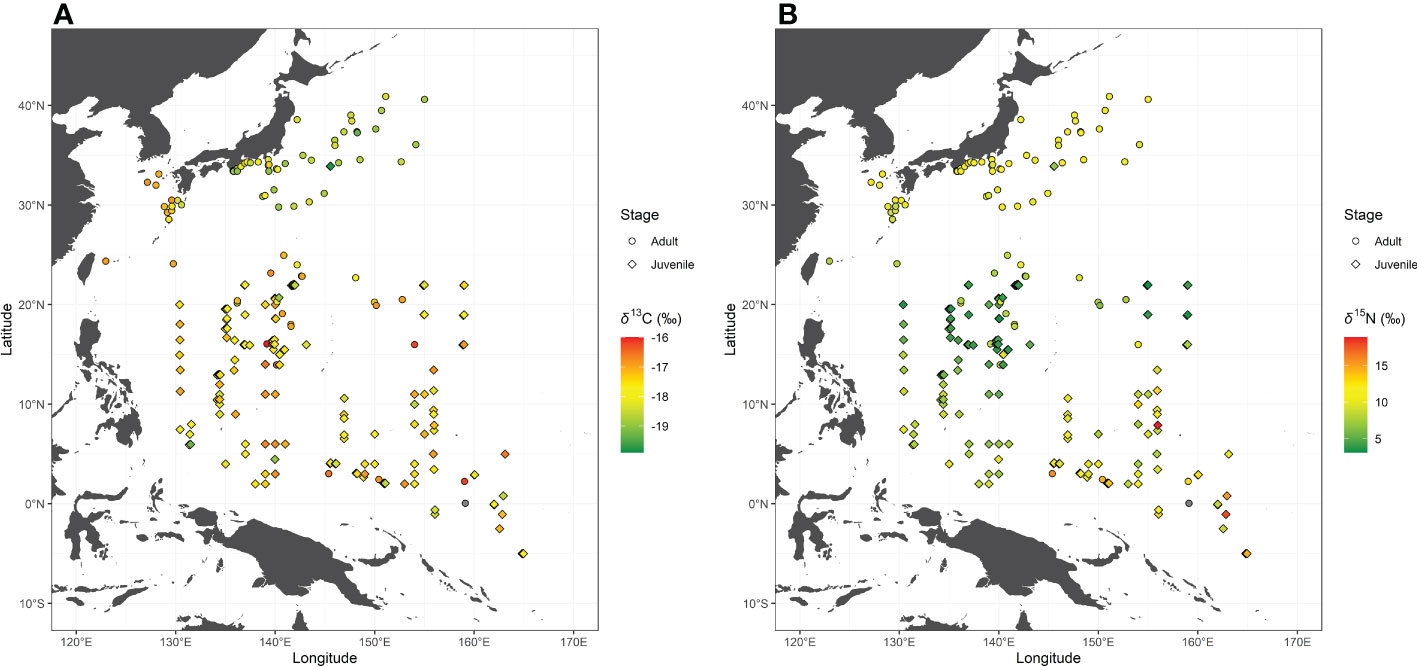
Figure 2 Bulk tissue carbon (δ13CBulk: A) and nitrogen (δ15NBulk: B) stable isotope ratios of skipjack tuna (Katsuwonus pelamis) in the western Pacific. Isotope ratios of skipjack of the same stage collected at the same location are averaged.
The best-fit model for δ15N included salinity, temperature, phosphate, and nitrate concentrations without smoothing, and fork length and iron concentration with smoothing (Supplementary Figures 1 and 2, Table 1). All sanity checks were positive for the best-fit model. The ΔAIC (the difference between the AIC for a model and the best-fit model) of the model with the second lowest AIC (ΔAIC2nd – Best) was 0.986, and the best-fit model accounted for 86.9% of the variation in observed δ15N values of skipjack muscle.
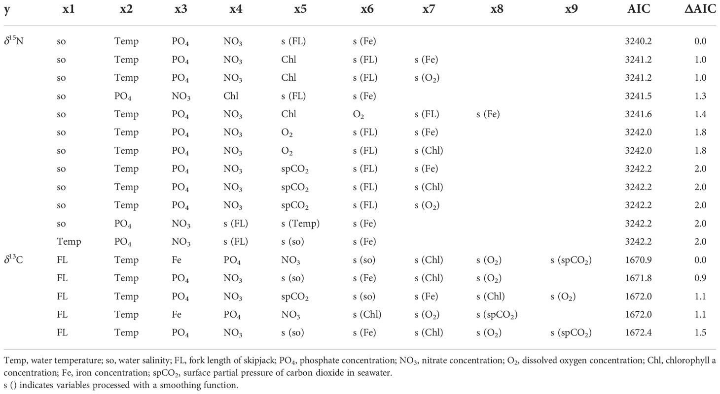
Table 1 Results of model selection based on the Akaike information criterion (AIC). Models with ΔAIC ≤ 2 are shown.
The best-fit model for δ13C included fork length, temperature, phosphate, nitrate, and iron concentrations without smoothing, and salinity, concentrations of chlorophyll a and dissolved oxygen, and the surface partial pressure of carbon dioxide with smoothing (Table 1). All sanity checks were positive for the best-fit model. The ΔAIC2nd – Best was 0.942, and the best-fit model accounted for 72.1% of the variation in observed δ13C values of skipjack muscle.
The δ15N and fork length of skipjack show a positive asymptotic relationship (Figure 3A), with a largely monotonous increase until fork length reaches 400 mm (0.01265‰/mm), approaching an asymptotic value at 600 mm (Δδ15N600mm–0mm = 5.84‰). Fork length with smoothing was included in all models with ΔAIC smaller than 2 for δ15N. The δ13C and fork length of skipjack showed a positive linear relationship (Supplementary Figure 2) with a small coefficient (0.00077‰/mm). Fork length without smoothing was included in all models with ΔAIC smaller than 2 for δ13C.
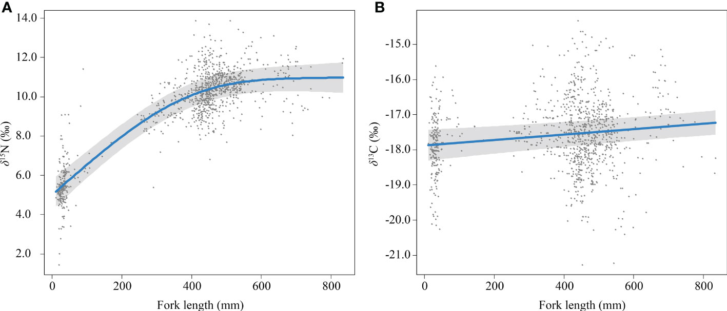
Figure 3 Relationship between fork length and δ15NBulk (A) and δ13CBulk (B) of skipjack tuna (Katsuwonus pelamis) in the western Pacific (blue lines) with randomized quantile partial residuals (gray areas) from the best-fit models. Each data point represents residuals from each data.
The western Pacific δ15N isoscape showed a clear latitudinal trend, with values in the WTP (from 10°S to 10–15°N) higher than in other northern regions (Figure 4). Overall, the uncertainty profile of δ15N was low around the sampling points, but high in the marginal region of our study area. On the other hand, δ13C was low in the WTNP (north of 20°N) and around the equator (from 2°S to 4°N) compared with the other regions. The uncertainty of estimated δ13C was low around the sampling points north of 4°N, but high in the marginal regions of the study area and south of 4°N regardless of the spatial density of sampling points.
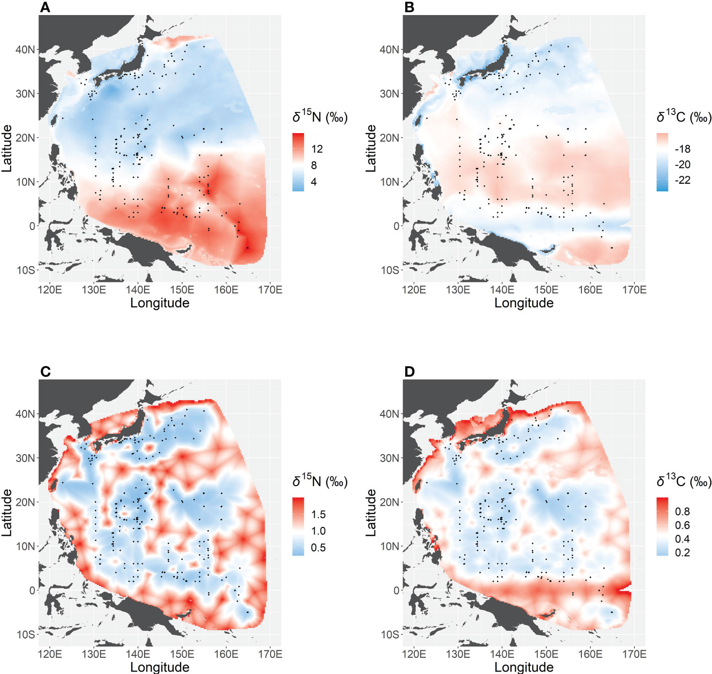
Figure 4 Isoscapes of nitrogen (A) and carbon (B) stable isotope ratios in the western Pacific, and the uncertainty (standard deviation) of predicted nitrogen (C) and carbon (D) isotope ratios estimated by simulation from the best-fit models (n = 500).
The results of compound-specific δ15N analysis for five skipjack samples representing the main regions (WTP, WSNP, and WTNP) with typical bulk-tissue isotope ratios are shown in Table 2. In summary, regional mean δ15NBulk was highest for WTP, followed by WTNP and WSNP, while TPGlu–Phe was highest for WTNP followed by WSNP and WTP. Thus, the trend in the regional variability of δ15NBulk was not consistent with that of TPGlu–Phe (Figure 5).
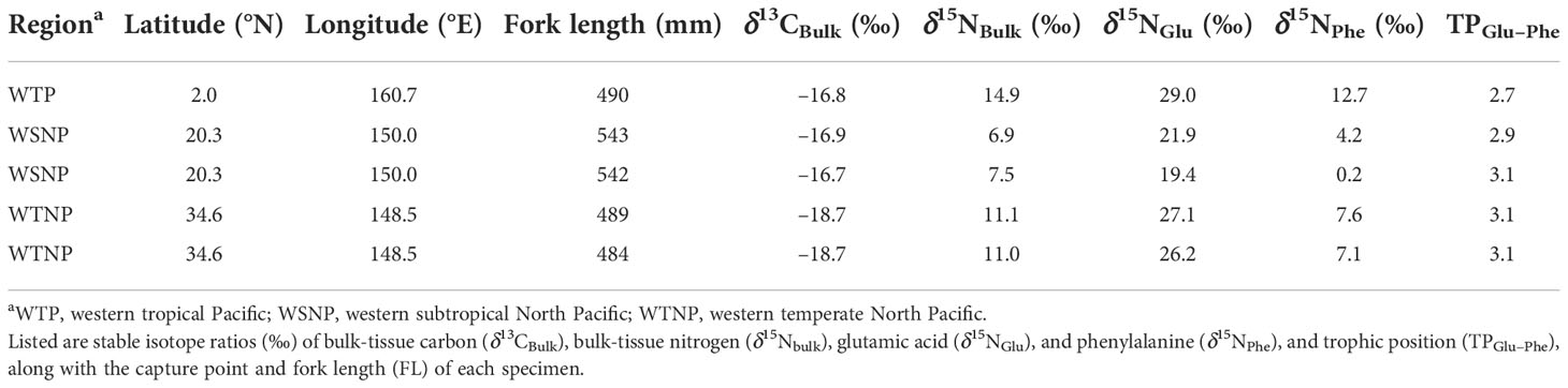
Table 2 Detailed sample information for five skipjack tuna (Katsuwonus pelamis) specimens used for compound-specific isotope analysis.
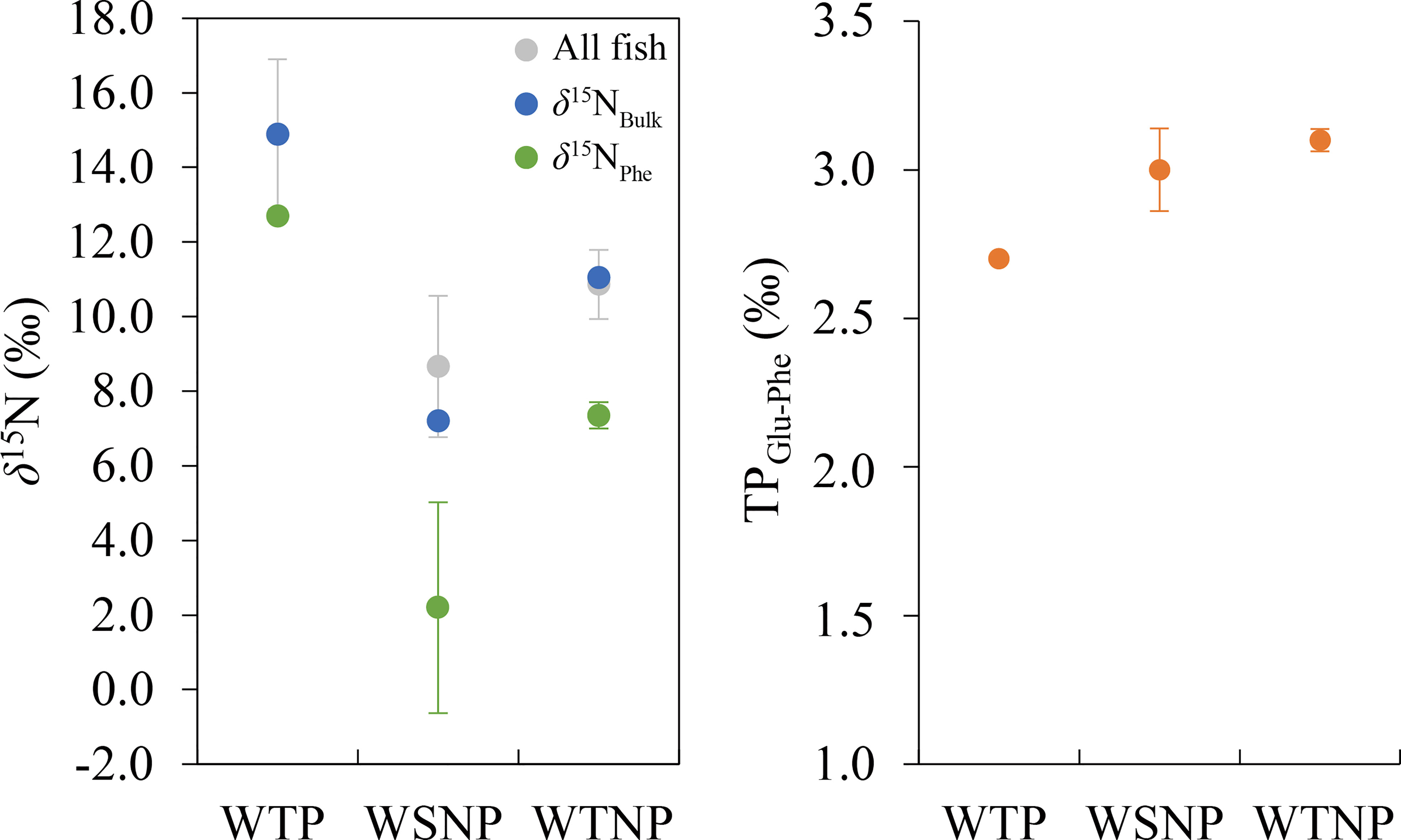
Figure 5 Mean δ15NBulk and δ15NPhe (left), and TPGlu–Phe (right) of skipjack tuna (Katsuwonus pelamis) in the western tropical Pacific (WTP), western subtropical North Pacific (WSNP), and western temperate North Pacific (WTNP). Gray, blue and green datapoints in the left panel indicate the mean (±SD) δ15NBulk of all skipjack samples, δ15NBulk and δ15NPhe of skipjack used for δ15NAAs, respectively. Orange datapoints in the right panel are the TPGlu–Phe of skipjack used for determining δ15NAAs.
For generation of isoscapes, previous studies have used species with lower mobility like jellyfish and copepods as proxy organisms (Trueman et al., 2017; Matsubayashi et al., 2020). The advantage of using other species with low swimming ability to create isoscape is that location-specific isotope ratios can be detected with high representativeness. On the other hand, the ontogenetic shift of isotope ratios in target fish and the offset of isotope ratios between target fish and isoscapes should be estimated separately in this method. This study used a target fish as a proxy organism for isoscapes, and successfully estimated both isoscapes (Figure 4) and the ontogenetic shifts of isotope ratios (Figure 3) of skipjack without compound-specific isotope analysis, through the use of geostatistical models. Furthermore, we can apply iso-logging of skipjack without considering the isotopic offset between isoscapes and target organism, because the isoscapes were generated based on the isotope ratios of the skipjack. Thus, our approach can be a useful alternative to the previous method, although our method has one drawback in that the uncertainty of isoscapes will increase with the number of fish captured that had migrated across regions with different isoscapes in the several months before they were caught. We addressed this issue by increasing the number of adult fish at each sampling point and period (Figure 1), and this may have contributed somewhat to decreasing the uncertainty of isoscapes given the high prediction ability of our models. Another solution would be to use juvenile fish only for generating isoscapes and then to construct another model to account for the ontogenetic shift of isotope ratios. However, this is not applicable when the distribution of juvenile and adult fish does not completely overlap, as with skipjack in the western Pacific where juvenile fish are scarce in the northern area (Lehodey et al., 2013). To minimize the uncertainty associated with a high migration ability of proxy organisms, it is important to use tissues with a high turnover rate. As of now, the fish tissue with the shortest stable isotope turnover time is epidermal mucus (Winter and Britton, 2021), but this is difficult to sample from juvenile fish smaller than 100 mm. Therefore, it is important to further explore turnover rates in other tissues to discover better ways to sample proxy organisms for generation of isoscapes.
Together with the results of the geostatistical models, our δ15NAAs data also show that the variation in isotope ratios of skipjack in the western Pacific was generally derived from the baseline shift of the isoscape and not from differences in prey items. Adult skipjack in the western Pacific are mainly piscivorous and occasionally consume cephalopods, with low selectivity for their prey (Iizuka et al., 1989). Therefore, regional shifts in prey abundance can cause regional differences in δ15NBulk. If the observed fluctuations of δ13CBulk and δ15NBulk in skipjack muscle resulted from differences in trophic position, the regional trend of δ15NBulk should be similar to that of TPGlu–Phe (Figure 5). However, our δ15NAAs data show that skipjack in the western Pacific have small individual variation in TPGlu–Phe (maximum difference: 0.4). Assuming that δ15NBulk increases 3.4‰ with trophic level (Minagawa and Wada, 1984), differences in TPGlu–Phe can only explain 1.4‰ of the observed variation of δ15NBulk out of 10.2‰ (Table 2, Figure 5). Given that the δ15NPhe, which generally has a small trophic discrimination factor (about 0.4%; Chikaraishi et al., 2009), was more correlated with δ15NBulk of skipjack muscle than TPGlu–Phe, individual differences in δ15NBulk of adult skipjack largely reflect the variation of δ15N at the base of the food web.
TPGlu–Phe of skipjack estimated by commonly used TDFGlu-Phe (7.6 ‰) were somewhat lower (2.7–3.1) than the trophic position estimated by stomach-content analysis (TPSCA = 3.8; Bradley et al., 2015). Although the optimal TDFGlu–Phe to use for estimating the trophic position of skipjack remains controversial (e.g., Bradley et al., 2015; McMahon and McCarthy, 2016; Ohkouchi et al., 2017; Coletto et al., 2022), differences in TPGlu–Phe of skipjack do not affect intraspecific variation in TDFGlu–Phe, and thus would not affect our conclusion that regional variation in TDFGlu–Phe are unlikely to explain δ15NBulk differences among regions.
Regional differences in δ15N of skipjack in the western Pacific were largely consistent with the δ15N distribution of nitrate in this region (Rafter et al., 2019). Low δ15N around 10°N to 35°N (Figure 4) is related to extensive N2 fixation in this region (Gruber, 2016), because N2 fixers typically exhibit lower δ15N values than non-N2 fixers (McClelland et al., 2003). On the other hand, our isoscape suggests that the low-δ15N area extends as far as 40°N, which is not consistent with known distributions of N2 fixers or low nitrate δ15N (Gruber, 2016; Rafter et al., 2019). Presumably, this inconsistency is attributable to the relatively longer turnover time of skipjack muscle. The area around 35–40°N is the northern limit of skipjack migration and they can stay there at most four months a year (from June to September; Mugo et al., 2011; Kiyofuji et al., 2019a). Given that the turnover time of adult skipjack white muscle is about four months, isotope ratios of the muscle of skipjack captured around 35–40°N are likely to reflect the low δ15N values south of 35°N, and thus our isoscape shows low δ15N up to 40°N. On the other hand, the high δ15N south of 10–15°N can be explained by high nitrate utilization and limited N2 fixation. In the surface layer of the tropical Pacific Ocean, a strong halocline above the thermocline generates a barrier layer, which impedes vertical mixing and nutrient supply from subsurface to surface waters (Sprintall & Tomczak, 1992). The limited nutrient influx results in high nitrate utilization (i.e. low nitrate concentration)—the ratio of nitrate assimilation by phytoplankton to nitrate supply in the euphotic layer—and nitrate δ15N increases with nitrate depletion (Yoshikawa et al., 2018). Furthermore, N2 fixation is limited in this region (Gruber, 2016; Tanita et al., 2021) mainly due to the depleted dissolved iron concentration (Tanita et al., 2021). Such biogeochemical factors result in a clear latitudinal trend in δ15N, rendering it useful for segregating the habitat use of skipjack in the western Pacific.
Interpretation of spatial variation in δ13C is much more difficult than that of δ15N. The spatial variations in δ13C of skipjack muscle should be ultimately determined by that of phytoplankton (δ13Cphy), which is strongly influenced by the δ13C of dissolved inorganic carbon (DIC) and the isotopic fractionation associated with carbon uptake (Tuerena et al., 2019). In the case of the western Pacific, there are no clear latitudinal differences in δ13C of DIC (Quay et al., 2003), and therefore the spatial variation in the δ13C isoscape would be driven by the uptake fractionation by phytoplankton. Until the early 1990s, the δ13C of phytoplankton was thought to be determined by the DIC concentration in the ambient water (Sackett et al., 1965; Rau et al., 1991). Our geostatistical model also predicted an inverse relationship between DIC and δ13C (Supplementary Figure 2), and the belt-shaped low-δ13C zone around the equator (Figure 4) may be mainly due to the high spCO2 in this region (Supplementary Figure 3). However, there is a large uncertainty associated with the equatorial low-δ13C zone and further sampling in this region would provide important clarification (Figure 4). On the other hand, the clear δ13C gradient around 20°N is not likely explained by spatial variation in spCO2. Recent studies have shown that local differences in phytoplankton species composition can be important controls on δ13Cphy (e.g. Francois et al., 1993; Bidigare et al., 1997; Popp et al., 1998; Tuerena et al., 2019) as well as the DIC concentration, specifically in regions where the DIC is not high and is less variable, as in the western Pacific (Supplementary Figure 3). Thus, we presume that local differences in environmental variables altered the phytoplankton species composition, and ultimately generated spatial variation in δ13C of skipjack muscle in this region. It is worth noting that anthropogenic CO2 emission can be another factor influencing the spatial variation in δ13Cphy (Tuerena et al., 2019).
In this study, we demonstrated that δ13C and δ15N measurements of skipjack in the western Pacific can help to identify their latitudinal migration. Because the dorsal muscle, which is a major tissue used for isotope analysis of fishes, only represents isotope ratios at a specific point in time, the utility of isoscapes will be maximized when they are used along with the isotopic analysis of incremental growth tissues such as eye lenses and vertebral bone (e.g. Quaeck-Davies et al., 2018; Matsubayashi et al., 2019). Iso-logging using such incremental growth tissue would allow us to understand how skipjack in this region utilize different habitats though their lifetime without using electronic tags. For example, if time series isotopic data for eye lens are available, the migration pattern can be tracked by the following steps: i) calculate the fork length when each layer is formed from the equation relating lens diameter to fork length, ii) using the equation relating fork length to isotopic ratios (Figure 3), correct the isotope ratios of eye lens so that the fork length is at zero; iii) subtract Δδ15Nmuscle - eye lens from the value obtained in ii), iv) corrected lens isotope ratios can then be compared to the isoscape (Figure 4). We also suggest that the isoscapes generated in this study can be applied to other fish species that migrate in the western Pacific Ocean, such as albacore Thunnus alalunga (Nikolic et al., 2017), Pacific bluefin tuna Thunnus orientalis (Fujioka et al., 2018), and Japanese eel Anguilla japonica (Aoyama et al., 2014). For these other target species, however, it will be necessary to apply an appropriate correction to the trophic discrimination factor for differences between skipjack muscle and specific tissues of these other species. By using this method, we can better understand the immigration/emigration rates and connectivity in each region, which is crucial for cooperative management of shared fish stocks like skipjack. Further studies to generate precise isoscapes of δ13C and δ15N based on ocean models hold promise for improving the spatiotemporal resolution of isotope tracking and, together with the results of this study, will facilitate its use.
The original contributions presented in the study are included in the article/Supplementary Material. Further inquiries can be directed to the corresponding author.
JM and HM conceived this study. HM and YT provided skipjack samples and contextual information. HM, YC, NO, KK, NFI, and NOO performed bulk and compound-specific stable isotope analyses. JM performed statistical analyses and wrote the first draft of the paper. All authors contributed to the article and approved the submitted version.
This study was partially supported by the Foundation for the Japan Society for the Promotion of Science (JSPS) KAKENHI Grants 19H04247, 21H03579, 21H04784, and 22H05028 to JM, and 20H00208 to NO, and the Research and Assessment Program for Fisheries Resources of the Fisheries Agency of Japan.
This study was conducted with the support of the Joint Research Grant for the Environmental Isotope Study of the Research Institute for Humanity and Nature. We thank H. Ashida, S. Ohashi, F. Tanaka, and H. Kiyofuji at the Fisheries Resources Institute, Japan Fisheries Research and Education Agency, for their help with sample collection. We thank C. Yoshikawa at the Japan Agency for Marine-Earth Science and Technology for her helpful comments on a draft of this manuscript. We also thank the reviewers for their prompt and careful review of our draft and for their helpful comments.
The authors declare that the research was conducted in the absence of any commercial or financial relationships that could be construed as a potential conflict of interest.
All claims expressed in this article are solely those of the authors and do not necessarily represent those of their affiliated organizations, or those of the publisher, the editors and the reviewers. Any product that may be evaluated in this article, or claim that may be made by its manufacturer, is not guaranteed or endorsed by the publisher.
The Supplementary Material for this article can be found online at: https://www.frontiersin.org/articles/10.3389/fmars.2022.1049056/full#supplementary-material
Anderson S. C., Ward E. J., English P. A., Barnett L. A. K. (2022). sdmTMB: An r package for fast, flexible, and user-friendly generalized linear mixed effects models with spatial and spatiotemporal random fields. bioRxiv 2022.03.24.485545. doi: 10.1101/2022.03.24.485545
Aoyama J., Watanabe S., Miller M. J., Mochioka N., Otake T., Yoshinaga T., et al. (2014). Spawning sites of the Japanese eel in relation to oceanographic structure and the West Mariana ridge. PloS One 9, e88759. doi: 10.1371/journal.pone.0088759
Barrett I., Hester F. J. (1964). Body temperature of yellowfin and skipjack tunas in relation to sea surface temperature. Nature 203, 96–97. doi: 10.1038/203096b0
Bartoo N. W. (1987). “Tuna and billfish summaries of major stocks,” in Administrative report LJ-87-26 (La Jolla: National Marine Fisheries Service).
Bidigare R. R., Fluegge A., Freeman K. H., Hanson K. L., Hayes J. M., Hollander D., et al. (1997). Consistent fractionation of c-13 in nature and in the laboratory: Growth-rate effects in some haptophyte algae. Global Biogeochem. Cy. 11, 279–292. doi: 10.1029/96gb03939
Bradley C. J., Wallsgrove N. J., Choy C. A., Drazen J. C., Hetherington E. D., Hoen D. K., et al. (2015). Trophic position estimates of marine teleosts using amino acid compound specific isotopic analysis. Limnol. Oceanogr. Meth. 13, 476–493. doi: 10.1002/lom3.10041
Caddy J. F. (1997). “Establishing a consultative mechanism or arrangement for managing shared stocks within the jurisdiction of contiguous states,” in Taking stock: Defining and managing shared resources, Australian society for fish biology and aquatic resource management association of Australasia joint workshop proceedings, vol. 15 . Ed. Hancock D. A. (Sydney: Australian Society for Fish Biology), 81–123.
Canseco J. A., Niklitschek E. J., Harrod C. (2021). Variability in δ13C and δ15N trophic discrimination factors for teleost fishes: A meta-analysis of temperature and dietary effects. Rev. Fish. Biol. Fish. 32, 313–329. doi: 10.1007/s11160-021-09689-1
Carey F. G., Teal J. M. (1969). Regulation of body temperature by the bluefin tuna. Comp. Biochem. Physiol. 28, 205–213. doi: 10.1016/0010-406X(69)91336-X
Carvalho F., Ahrens R., Murie D., Bigelow K., Aires-Da-Silva A., Maunder M. N., et al. (2015). Using pop-up satellite archival tags to inform selectivity in fisheries stock assessment models: A case study for the blue shark in the south Atlantic ocean. ICES. J. Mar. Sci. 72, 1715–1730. doi: 10.1093/icesjms/fsv026
Chikaraishi Y., Ogawa N. O., Kashiyama Y., Takano Y., Suga H., Tomitani A., et al. (2009). Determination of aquatic food-web structure based on compound-specific nitrogen isotopic composition of amino acids. Limnol. Oceanogr. Meth. 7, 740–750. doi: 10.4319/lom.2009.7.740
Chikaraishi Y., Steffan S. A., Takano Y., Ohkouchi N. (2015). Diet quality influences isotopic discrimination among amino acids in an aquatic vertebrate. Ecol. Evol. 5, 2048–2059. doi: 10.1002/ece3.1491
Coletto J. L., Besser A. C., Botta S., Madureira L. A. S. P., Newsome S. D. (2022). Multi-proxy approach for studying the foraging habitat and trophic position of a migratory marine consumer in the southwestern Atlantic ocean. Mar. Ecol. Prog. Ser. 690, 147–163. doi: 10.3354/meps14036
Coletto J. L., Botta S., Fischer L. G., Newsome S. D., Madureira L. S. (2021). Isotope-based inferences of skipjack tuna feeding ecology and movement in the southwestern Atlantic ocean. Mar. Environ. Res. 165, 105246. doi: 10.1016/j.marenvres.2020.105246
Cooke S. J., Woodley C. M., Eppard M. B., Brown R. S., Nielsen J. L. (2011). Advancing the surgical implantation of electronic tags in fish: A gap analysis and research agenda based on a review of trends in intracoelomic tagging effects studies. Rev. Fish. Biol. Fish. 21, 127–151. doi: 10.1007/s11160-010-9193-3
Francois R., Altabet M. A., Goericke R., McCorkle D. C., Brunet C., Poisson A. (1993). Changes in the delta c-13 of surface water particulate organic matter across the subtropical convergence in the SW Indian ocean. Global Biogeochem. Cy. 7, 627–644. doi: 10.1029/93GB01277
Fry B., Sherr E. (1984). δ13C measurements as indicators of carbon flow in marine and freshwater ecosystems. Contrib. Mar. Sci. 27, 49–63. doi: 10.1007/978-1-4612-3498-2_12
Fujioka K., Fukuda H., Tei Y., Okamoto S., Kiyofuji H., Furukawa S., et al. (2018). Spatial and temporal variability in the trans-pacific migration of pacific bluefin tuna (Thunnus orientalis) revealed by archival tags. Prog. Oceanogr. 162, 52–65. doi: 10.1016/j.pocean.2018.02.010
Graham B. S., Koch P. L., Newsome S. D., McMahon K. W., Aurioles D. (2010). “Using isoscapes to trace the movements and foraging behavior of top predators in oceanic ecosystems,” in Isoscapes. Eds. West J., Bowen G., Dawson T., Tu K. (Dordrecht: Springer), 299–318.
Graham B. S., Grubbs D., Holland K., Popp B. N. (2007). A rapid ontogenetic shift in the diet of juvenile yellowfin tuna from Hawaii. Mar. Biol. 150, 647–658. doi: 10.1007/s00227-006-0360-y
Graves J. E., Horodysky A. Z. (2015). Challenges of estimating post-release mortality of istiophorid billfishes caught in the recreational fishery: A review. Fish. Res. 166, 163–168. doi: 10.1016/j.fishres.2014.10.014
Gruber N. (2016). Elusive marine nitrogen fixation. Proc. Natl. Acad. Sci. U.S.A. 113, 4246–4248. doi: 10.1073/pnas.1603646113
Hebblewhite M., Haydon D. T. (2010). Distinguishing technology from biology: A critical review of the use of GPS telemetry data in ecology. Philos. Trans. R. Soc B. 365, 2303–2312. doi: 10.1098/rstb.2010.0087
Hoyle S., Kleiber P., Davies N., Langley A., Hampton J. (2011). “Stock assessment of skipjack tuna in the Western and central pacific ocean,” in WCPFC-SC7-2011/SA-WP-04 (Pohnpei, Federated States of Micronesia: Western and Central Pacific Fisheries Commission, Seventh Regular Session).
Hsieh Y., Shiao J. C., Lin S. W., Iizuka Y. (2019). Quantitative reconstruction of salinity history by otolith oxygen stable isotopes: An example of a euryhaline fish Lateolabrax japonicus. Rapid Commun. Mass. Spectrom. 33, 1344–1354. doi: 10.1002/rcm.8476
Iizuka K., Asano M., Naganuma A. (1989). Feeding habits of skipjack tuna (Katsuwonus pelamis Linnaeus) caught by pole and line and the state of young skipjack tuna distribution in the tropical seas of the Western pacific ocean. Bull. Tohoku. Reg. Fish. Res. Lab. 51, 107–116.
Jepsen N., Koed A., Thorstad E., Baras E. (2002). Surgical implantation of transmitters in fish: How much have we learned? Hydrobiologia 483, 239–248. doi: 10.1007/978-94-017-0771-8_28
Jepsen N., Thorstad E. B., Havn T., Lucas M. C. (2015). The use of external electronic tags on fish: an evaluation of tag retention and tagging effects. Anim. Biotelem. 3, 49. doi: 10.1186/s40317-015-0086-z
Kiyofuji H., Aoki Y., Kinoshita J., Ohashi S., Fujioka K. (2019b). “A conceptual model of skipjack tuna in the western and central pacific ocean (WCPO) for the spatial structure configuration,” in WCPFC-SC15-2019/SA-WP-11 (Pohnpei, Federated States of Micronesia: Western and Central Pacific Fisheries Commission), 2019, 23.
Kiyofuji H., Aoki Y., Kinoshita J., Okamoto S., Masujima M., Matsumoto T., et al. (2019a). Northward migration dynamics of skipjack tuna (Katsuwonus pelamis) associated with the lower thermal limit in the western pacific ocean. Prog. Oceanogr. 175, 55–67. doi: 10.1016/j.pocean.2019.03.006
Kiyofuji H., Ochi D. (2016). Proposal of alternative spatial structure for skipjack stock assessment in the WCPO. Twelfth. Session. Sci. Committee., 3–11.
Kraska J., Crespo G. O., Johnston D. W. (2015). Bio-logging of marine migratory species in the law of the sea. Mar. Policy 51, 394–400. doi: 10.1016/j.marpol.2014.08.016
Lehodey P., Senina I., Calmettes B., Hampton J., Nicol S. (2013). Modelling the impact of climate change on pacific skipjack tuna population and fisheries. Clim. Change 119, 95–109. doi: 10.1007/s10584-012-0595-1
Lindgren F., Rue H., Lindström J. (2011). An explicit link between Gaussian fields and Gaussian Markov random fields: The stochastic partial differential equation approach. J. R. Stat. Soc Ser. A. Stat. Soc 73, 423–498. doi: 10.1111/j.1467-9868.2011.00777.x
Matsubayashi J., Osada Y., Tadokoro K., Abe Y., Yamaguchi A., Shirai K., et al. (2020). Tracking long-distance migration of marine fishes using compound-specific stable isotope analysis of amino acids. Ecol. Lett. 23, 881–890. doi: 10.1111/ele.13496
Matsubayashi J., Saitoh Y., Osada Y., Uehara Y., Habu J., Sasaki T., et al. (2017). Incremental analysis of vertebral centra can reconstruct the stable isotope chronology of teleost fishes. Methods Ecol. Evol. 8, 1755–1763. doi: 10.1111/2041-210X.12834
Matsubayashi J., Umezawa Y., Matsuyama M., Kawabe R., Mei W., Wan X., et al. (2019). Using segmental isotope analysis of teleost fish vertebrae to estimate trophic discrimination factors of bone collagen. Limnol. Oceanogr. Meth. 17, 87–96. doi: 10.1002/lom3.10298
McClelland J. W., Holl C. M., Montoya J. P. (2003). Relating low δ15N values of zooplankton to N2-fixation in the tropical north Atlantic: Insights provided by stable isotope ratios of amino acids. Deep. Sea. Res. Part I. Oceanogr. Res. Papers. 50, 849–861. doi: 10.1016/S0967-0637(03)00073-6
McMahon K. W., McCarthy M. D. (2016). Embracing variability in amino acid δ15N fractionation: Mechanisms, implications, and applications for trophic ecology. Ecosphere 7, e01511. doi: 10.1002/ecs2.1511
McWhinnie S. F. (2009). The tragedy of the commons in international fisheries: An empirical examination. J. Environ. Econ. Manage. 57, 321–333. doi: 10.1016/j.jeem.2008.07.008
Miller K. A., Munro G. R. (2004). Climate and cooperation: A new perspective on the management of shared fish stocks. Mar. Res. Econ. 19, 367–393. doi: 10.1086/mre.19.3.42629440
Minagawa M., Wada E. (1984). Stepwise enrichment of 15N along food chains: Further evidence and the relation between δ15N and animal age. Geochim. Cosmochim. Acta 48, 1135–1140. doi: 10.1016/0016-7037(84)90204-7
Mugo R., Saitoh S. I., Nihira A., Kuroyama T. (2010). Habitat characteristics of skipjack tuna (Katsuwonus pelamis) in the western north pacific: A remote sensing perspective. Fish. Oceanogr. 19, 382–396. doi: 10.1111/j.1365-2419.2010.00552.x
Mugo R., Saitoh S., Nihira A., Kuroyama T. (2011). “Application of multi-sensor satellite and fishery data, statistical models and marine GIS to detect habitat preferences of skipjack tuna,” in Handbook of satellite remote sensing image interpretation: Applications for marine living resources conservation and management. Eds. Morales J., Stuart V., Platt T., Sathyendranath S. (Dartmouth, Canada: EU PRESPO and IOCCG), 166–185.
Nikolic N., Morandeau G., Hoarau L., West W., Arrizabalaga H., Hoyle S., et al. (2017). Review of albacore tuna, Thunnus alalunga, biology, fisheries and management. Rev. Fish. Biol. Fish. 27, 775–810. doi: 10.1007/s11160-016-9453-y
Nishikawa H., Nishikawa S., Ishizaki H., Wakamatsu T., Ishikawa Y. (2020). Detection of the oyashio and kuroshio fronts under the projected climate change in the 21st century. Prog. Earth Planet. Sci. 7, 29. doi: 10.1186/s40645-020-00342-2
Ohkouchi N., Chikaraishi Y., Close H. G., Fry B., Larsen T., Madigan D. J., et al. (2017). Advances in the application of amino acid nitrogen isotopic analysis in ecological and biogeochemical studies. Org. Geochem. 113, 150–174. doi: 10.1016/j.orggeochem.2017.07.009
Popova E., Vousden D., Sauer W. H., Mohammed E. Y., Allain V., Downey-Breedt N., et al. (2019). Ecological connectivity between the areas beyond national jurisdiction and coastal waters: Safeguarding interests of coastal communities in developing countries. Mar. Policy 104, 90–102. doi: 10.1016/j.marpol.2019.02.050
Popp B. N., Laws E. A., Bidigare R. R., Dore J. E., Hanson K. L., Wakeham S. G. (1998). Effect of phytoplankton cell geometry on carbon isotopic fractionation. Geochim. Cosmochim. Acta 62, 69–77. doi: 10.1016/S0016-7037(97)00333-5
Priede I. G., Solbé J. D. L., Nott J. E., O'Grady K. T., Cragg-Hine D. (1988). Behaviour of adult Atlantic salmon, Salmo salar l., in the estuary of the river ribble in relation to variations in dissolved oxygen and tidal flow. J. Fish. Biol. 33, 133–139. doi: 10.1111/j.1095-8649.1988.tb05567.x
Quaeck-Davies K., Bendall V. A., MacKenzie K. M., Hetherington S., Newton J., Trueman C. N. (2018). Teleost and elasmobranch eye lenses as a target for life-history stable isotope analyses. PeerJ 6, e4883. doi: 10.7717/peerj.4883
Quay P., Sonnerup R., Westby T., Stutsman J., McNichol A. (2003). Changes in the 13C/12C of dissolved inorganic carbon in the ocean as a tracer of anthropogenic CO2 uptake. Global Biogeochem. Cy. 17, 1004. doi: 10.1029/2001GB001817
Rafter P. A., Bagnell A., Marconi D., DeVries T. (2019). Global trends in marine nitrate n isotopes from observations and a neural network-based climatology. Biogeosciences 16, 2617–2633. doi: 10.5194/bg-16-2617-2019
Rau G. H., Froelich P. N., Takahashi T., Des Marais D. J. (1991). Does sedimentary organic d13C record variations in quaternary ocean [CO2(aq)]? Paleoceanography 6, 335–347. doi: 10.1029/91pa00321
R Core Team (2021). R: A language and environment for statistical computing (Vienna, Austria: R Foundation for Statistical Computing). Available at: https://www.R-project.org/.
Rue H., Martino S., Chopin N. (2009). Approximate Bayesian inference for latent Gaussian models by using integrated nested Laplace approximations. J. R. Stat. Soc Ser. B. 71, 319–392. doi: 10.1111/j.1467-9868.2008.00700.x
Sackett W. M., Eckelmann W. R., Bender M. L., Be A. W. H. (1965). Temperature dependence of carbon isotope composition in marine plankton and sediments. Science 148, 235–237. doi: 10.1126/science.148.3667.23
Sakamoto T., Komatsu K., Shirai K., Higuchi T., Ishimura T., Setou T., et al. (2019). Combining microvolume isotope analysis and numerical simulation to reproduce fish migration history. Methods Ecol. Evol. 10, 59–69. doi: 10.1111/2041-210X.13098
Sippel T., Eveson J. P., Galuardi B., Lam C., Hoyle S., Maunder M., et al. (2015). Using movement data from electronic tags in fisheries stock assessment: A review of models, technology and experimental design. Fish. Res. 163, 152–160. doi: 10.1016/j.fishres.2014.04.006
Sprintall J., Tomczak M. (1992). Evidence of the barrier layer in the surface layer of the tropics. J. Geophys. Res. Oceans. 97, 7305–7316. doi: 10.1029/92JC00407
St John Glew K., Espinasse B., Hunt B.P., Pakhomov E.A., Bury S.J., Pinkerton M., et al. (2021). Isoscape models of the Southern Ocean: Predicting spatial and temporal variability in carbon and nitrogen isotope compositions of particulate organic matter. Glob. Biogeochem. Cycles35, e2020GB006901. doi: 10.1029/2020GB006901
Stevens E. D., Lam H. M., Kendall J. (1974). Vascular anatomy of the counter-current heat exchanger of skipjack tuna. J. Exp. Biol. 61, 145–153. doi: 10.1242/jeb.61.1.145
Tanita I., Shiozaki T., Kodama T., Hashihama F., Sato M., Takahashi K., et al. (2021). Regionally variable responses of nitrogen fixation to iron and phosphorus enrichment in the pacific ocean. J. Geophys. Res. Biogeosci. 126, e2021JG006542. doi: 10.1029/2021JG006542
Thorson J. T. (2019). Guidance for decisions using the vector autoregressive spatio-temporal (VAST) package in stock, ecosystem, habitat and climate assessments. Fish. Res. 210, 143–161. doi: 10.1016/j.fishres.2018.10.013
Thorstad E. B., Rikardsen A. H., Alp A., Økland F. (2013). The use of electronic tags in fish research–an overview of fish telemetry methods. Turk. J. Fish. Aquat. Sci. 13, 881–896. doi: 10.4194/1303-2712-v13_5_13
Trueman C. N., MacKenzie K. M., Palmer M. R. (2012). Identifying migrations in marine fishes through stable-isotope analysis. J. Fish. Biol. 81, 826–847. doi: 10.1111/j.1095-8649.2012.03361.x
Trueman C. N., MacKenzie K. M., St. John Glew K. (2017). Stable isotope-based location in a shelf sea setting: Accuracy and precision are comparable to light-based location methods. Methods Ecol. Evol. 8, 232–240. doi: 10.1111/2041-210X.12651
Tuerena R. E., Ganeshram R. S., Humphreys M. P., Browning T. J., Bouman H., Piotrowski A. P. (2019). Isotopic fractionation of carbon during uptake by phytoplankton across the south Atlantic subtropical convergence. Biogeosciences 16, 3621–3635. doi: 10.5194/bg-16-3621-2019
Vatsov M. (2016). Changes in the geographical distribution of shared fish stocks and the mackerel war: Confronting the cooperation maze. Scottish. Centre. Int. Law. Working. Paper. Ser. 13. doi: 10.2139/ssrn.2863853
Vecchio J. L., Peebles E. B. (2020). Spawning origins and ontogenetic movements for demersal fishes: An approach using eye-lens stable isotopes. Estuar. Coast. Shelf. Sci. 246, 107047. doi: 10.1016/j.ecss.2020.107047
Winter J. D. (1983). “Underwater biotelemetry,” in Fisheries techniques. Eds. Nielsen L. A., Johnson D. L. (Bethesda, Maryland: American Fisheries Society), 371–395.
Winter E. R., Britton J. R. (2021). Individual variability in stable isotope turnover rates of epidermal mucus according to body size in an omnivorous fish. Hydrobiologia 848, 363–370. doi: 10.1007/s10750-020-04444-2
Wood S. N. (2003). Thin plate regression splines. J. R. Stat. Soc Ser. B. Stat. Meth. 65, 95–114. doi: 10.1111/1467-9868.00374
Keywords: iso-logging, isoscape, ontogenetic shift, skipjack tuna, δ 13 C, δ 15 N, compound-specific isotope analysis
Citation: Matsubayashi J, Kimura K, Ohkouchi N, Ogawa NO, Ishikawa NF, Chikaraishi Y, Tsuda Y and Minami H (2022) Using geostatistical analysis for simultaneous estimation of isoscapes and ontogenetic shifts in isotope ratios of highly migratory marine fish. Front. Mar. Sci. 9:1049056. doi: 10.3389/fmars.2022.1049056
Received: 20 September 2022; Accepted: 26 October 2022;
Published: 28 November 2022.
Edited by:
Tomihiko Higuchi, The University of Tokyo, JapanReviewed by:
Julie Vecchio, South Carolina Department of Natural Resources, United StatesCopyright © 2022 Matsubayashi, Kimura, Ohkouchi, Ogawa, Ishikawa, Chikaraishi, Tsuda and Minami. This is an open-access article distributed under the terms of the Creative Commons Attribution License (CC BY). The use, distribution or reproduction in other forums is permitted, provided the original author(s) and the copyright owner(s) are credited and that the original publication in this journal is cited, in accordance with accepted academic practice. No use, distribution or reproduction is permitted which does not comply with these terms.
*Correspondence: Jun Matsubayashi, bWF0c3VqQGZyYS5hZmZyYy5nby5qcA==
Disclaimer: All claims expressed in this article are solely those of the authors and do not necessarily represent those of their affiliated organizations, or those of the publisher, the editors and the reviewers. Any product that may be evaluated in this article or claim that may be made by its manufacturer is not guaranteed or endorsed by the publisher.
Research integrity at Frontiers
Learn more about the work of our research integrity team to safeguard the quality of each article we publish.