Absorption-based algorithm for satellite estimating the particulate organic carbon concentration in the global surface ocean

Particulate organic carbon (POC) in the surface ocean contributes to understanding the global ocean carbon cycle system. The surface POC concentration can be effectively detected using satellites. In open oceans, the blue-to-green band ratio (BG) algorithm is often used to obtain global surface ocean POC concentrations. However, POC concentrations are underestimated in waters with complex optical environments. To generate a more accurate global POC mapping in the surface ocean, we developed a new ocean color algorithm using a mixed global-scale in situ POC dataset with the concentration ranging from 11.10 to 4389.28 mg/m³. The new algorithm (a-POC) was established to retrieve the POC concentration using the strong relationship between the absorption coefficient at 490 nm (a(490)) and POC, in which a(490) was from the Ocean Color Climate Change Initiative (OC-CCI) v5.0 suite. Afterward, the a-POC algorithm was applied to OC-CCI v5.0 data for special regions and the global ocean. The performances of the a-POC algorithm and the BG algorithm were compared by combining the match-ups of satellite data and in situ dataset. The results showed that the statistical parameters of the a-POC algorithm were similar to those of the BG algorithm in the Atlantic oligotrophic gyre regions, with a median absolute percentage deviation (MAPD) value of 22.04%. In the eastern coastal waters of the United States and the Chesapeake Bay, the POC concentration retrieved by the a-POC algorithm was highly consistent with the match-ups, and MAPD values were 33.06% and 26.11%. The a-POC algorithm was also applied to the Ocean and Land Color Instrument (OLCI) data pre-processed with different atmospheric correction algorithms to evaluate the universality. The result showed that the a-POC algorithm was robust and less sensitive to atmospheric correction than the BG algorithm.

1 Introduction

The ocean is a vast carbon reservoir, and the ocean carbon cycle is crucial in studying global climate change and environmental evolution (Hedges, 1992; Siegenthaler and Sarmiento, 1993). Particulate organic carbon (POC) and dissolved organic carbon (DOC) are two kinds of oceanic organic carbon (Amon and Benner, 1996; Jahnke, 1996; Chen et al., 2022). Although the stock of POC is small, its importance depends on its constituents (phytoplankton, bacteria, zooplankton, and organic detritus), which are responsible for relatively large carbon fluxes and short turnaround times (Stramska, 2009; Evers-King et al., 2017). In addition, POC is also an important indicator of ocean primary productivity (Behrenfeld et al., 2005). The flux from dissolved inorganic carbon (DIC) to POC through primary production is estimated to be about 50 Gt C/year, accounting for about 50% of global primary production (Liu et al., 2021). Due to POC transformation (e.g., remineralization), sedimentation, physical mixing, and horizontal ocean current transport, the concentration of POC (mg/m³) in the surface ocean changes significantly on temporal and spatial scales (Field Christopher et al., 1998; Stramski et al., 1999; Gardner et al., 2006; Omand et al., 2015; Stramska and Cieszyńska, 2015). Therefore, the POC measured through traditional shipboard platforms or other in situ observation platforms cannot fully characterize POC changes on a global scale.

Ocean color remote sensing has the advantages of broad spatial coverage and long time series in obtaining bio-optical properties. It solves the drawback that the data obtained by traditional monitoring methods are dispersed in time and space. In the past few decades, ocean color remote sensing technology has been rapidly developed. For example, the Sea-viewing Wide-Field-of-view Sensor (SeaWiFS), Moderate Resolution Imaging Spectroradiometer (MODIS), Medium-Resolution Imaging Spectrometer (MERIS), Visible Infrared Imaging Radiometer Suite (VIIRS), and Ocean and Land Colour Instrument (OLCI) can send ocean color data to ground receiving stations almost every day. By applying specific retrieval algorithms to remote sensing data, ocean color remote sensing technology can obtain the distribution of oceanic POC concentrations on temporal and spatial scales (Loisel et al., 2002; Stramska and Stramski, 2005; Allison et al., 2010; Duforêt-Gaurier et al., 2010; Stramska, 2014; Stramska and Cieszyńska, 2015; Stramski et al., 2022).

Current POC concentration retrieval algorithms are mainly based on the inherent optical properties (IOPs), the apparent optical properties (AOPs), and water constituents (e.g., chlorophyll-a (Chla) and total suspended matter (TSM)). The first type is two-step algorithms based on IOPs. The relationship between AOPs and IOPs was first established, and then an empirical relationship between IOPs and POC concentration was formulated. These IOPs include the particulate backscattering coefficient (b_bp) and the particle beam attenuation coefficient (c_p). Stramski et al., 1999 used b_bp at 510 nm as a proxy to retrieve the POC concentration. Gardner et al., 2006 established a linear regression between c_p and the POC concentration to retrieve the POC concentration. However, the relationship between b_bp, c_p, and POC varied by sea area. At similar POC levels, the b_bp at 510 nm in the Antarctic Polar Front Zone was higher than that in the Ross Sea region, indicating a difference in the specific b_bp of carbon (Stramski et al., 1999; Stramski et al., 2001; Pabi and Arrigo, 2006; Stramski et al., 2008). Le et al., 2018 showed a relatively weak relationship between the POC concentration and the backscattering coefficient at 547 nm, and the coefficient of determination was 0.33. In addition, there is a significant change in the slope between c_p and POC concentrations (about twice as large) compared to the linear regression model for different sea areas worldwide (Gardner et al., 2006). Therefore, these algorithms may be limited in retrieving POC concentrations on a global scale.

The second type of algorithm obtains the POC concentration based on the empirical relationship between AOPs and the POC concentration. The typical empirical algorithm is the blue-to-green band ratio (BG) of remote sensing reflectance (R_rs(λ), where λ is the light wavelength) (Stramski et al., 2008). The BG algorithm outperformed the b_bp-based two-step algorithm in the open ocean (Stramski et al., 2008; Allison et al., 2010). It was used by the National Aeronautics and Space Administration (NASA) Ocean Biology Processing Group to generate global POC products. Le et al., 2018 proposed an empirical POC concentration retrieval algorithm (CI_POC) based on a three-band R_rs(λ) difference (i.e., Color Index) initially developed by Hu et al., 2012. However, the accuracy of empirical algorithms relies heavily on the variation of the in situ datasets used to establish the algorithms. The BG algorithm was established using in situ POC concentrations ranging from 12 to 270 mg/m³, and the CI_POC algorithm was established using in situ POC concentrations less than 1000 mg/m³. As a result, the BG and CI_POC algorithms had significant errors in coastal waters with complex optical environments (Duan et al., 2014; Evers-King et al., 2017; Le et al., 2017; Le et al., 2018; Lin et al., 2018; Jiang et al., 2019; Tran et al., 2019).

The third type of algorithm is based on the water constituents. Loisel et al., 2002 proposed a POC algorithm based on the combination of b_bp at 490 nm and Chla concentrations. However, this algorithm significantly underestimated the data in regions with high POC concentrations (Evers-King et al., 2017). In turbid regions such as coastal waters, the uncertain accuracy of Chla concentration retrieval can bring errors to further POC retrieval. Liu et al., 2019 established the relationship between TSM concentrations and POC concentrations using an in situ dataset collected in the Changjiang River Estuary. This relationship was verified through the Geostationary Ocean Color Imager (GOCI) data. As the relationship between TSM and POC is not static, the ratio of POC to TSM in different water environments is greatly affected by the relative contribution of organic and inorganic particulate matter (Bishop, 1999). The lack of a recognized ocean color TSM retrieval model also increases the difficulty of algorithm generalization (Yu et al., 2019; Liu et al., 2021).

Since Stramski et al., 1999 proposed the backscattering of particulate matter as a proxy for POC, ocean color retrieval algorithms for POC concentration based on IOPs have been continuously investigated. Previous studies have suggested that the absorption coefficient (a(λ)) can serve as a proxy for organic particulate matter, particularly the wavelength λ at longer blue bands (Woźniak et al., 2010; Le et al., 2018). However, few POC algorithms based on a(λ) have been studied, especially on the direct establishment of the relationship between POC and a(λ) (Jiang et al., 2019). Often, a(λ) is subdivided into the following four components:

$$\text{a}\left(\text{λ}\right)={\text{a}}_{\text{w}}\left(\text{λ}\right)+{\text{a}}_{\text{Φ}}\left(\text{λ}\right)+{\text{a}}_{\text{NAP}}\left(\text{λ}\right)+{\text{a}}_{\text{CDOM}}\left(\text{λ}\right)$$

Subscripts w, Φ, NAP, and CDOM represent pure seawater, phytoplankton, nonalgal particles, and colored dissolved organic matter. Selecting a(λ) as a proxy for POC can describe the variability in phytoplankton and nonalgal particles, although doing so also mingled with the signal of CDOM, especially in coastal waters. Since the absorption coefficient of CDOM (a_CDOM) decays exponentially with increasing wavelength (Babin et al., 2003), this study focused on the relationship between a(490) and POC concentration. The OC-CCI data was combined with a global in situ POC dataset to establish an absorption-coefficient-based POC concentration retrieval algorithm (a-POC). Afterward, the performance of the a-POC algorithm was compared with that of the BG algorithm on a global and regional scale, and an uncertainty map was plotted. Finally, the a-POC algorithm was applied to other sensors, and its universality was evaluated.

2 Data and methods

2.1 In situ dataset

The in situ POC dataset used in this study was obtained from globally shared databases and an independently collected Bohai Sea dataset. The shared databases mainly consisted of datasets collected by Martiny et al., 2014 in the Dryad Digital Repository (https://datadryad.org/) and a large number of datasets provided by contributors in SeaBASS (https://seabass.gsfc.nasa.gov) (Werdell and Bailey, 2005). The Bohai Sea dataset was collected in the Bohai Sea of China. It included optical and biochemical parameters of the ocean surface (e.g., R_rs(λ), the concentrations of Chla and POC). The water samples used to obtain biochemical parameters were collected at a depth of 0.5 m. R_rs(λ) and Chla were measured in the same way as in the study of Jiang et al., 2020, where the optical measurement followed the NASA optics protocols (Mueller et al., 2003), and Chla was measured by the fluorometric method (Cui et al., 2010). The measurement method for POC concentration was according to the method provided by Sharp, 1974. Before analysis, samples were collected using GF/F filters with a pore size of 0.7 µm and pre-combusted (450 °C) and dried overnight at 65 °C. Filters were acidified by adding low-carbon HCl directly or by overnight exposure to concentrated HCl solution fumes in a desiccator to remove interference from particulate inorganic carbon (Hedges and Stern, 1984). The filter was then dried at 55°C, loaded into pre-combusted tin capsules, and converted to organic carbon in an elemental analyzer at 960 °C. Finally, the POC concentrations were calculated by subtracting the average organic carbon mass (measured on blank filters) from the organic carbon mass (measured on filters) and dividing it by the volume of the filtered sample. POC concentrations could be easily overestimated due to the inevitable errors in POC measurements, especially from dissolved organic carbon adsorbed on the filter (Gardner et al., 2003). Therefore, POC concentrations below 10 mg/m³ were considered invalid in this study (Cetinić et al., 2012; Le et al., 2018). For shared databases that provide a sampling depth, the measurements from 10 m below the water surface were averaged to provide the “surface” value (Evers-King et al., 2017). The dataset was sampled from 1997 to 2020, with areas ranging from the open oceans to coastal waters, providing good representation on both temporal and spatial scales.

2.2 Satellite data

The European Space Agency (ESA) Ocean Color Climate Change Initiative (OC-CCI) project has produced a series of validated Essential Climate Variables (ECVs) with error characteristics by merging observational products from multiple satellite sensors. Since the first phase of OC-CCI was launched in 2010, several updates and improvements have been implemented, and the current OC-CCI project has progressed to version 5.0 (Sathyendranath et al., 2019; Sathyendranath et al., 2021). The OC-CCI v5.0 data is created by band-shifting (Mélin and Sclep, 2015) and bias-correcting SeaWiFS, MODIS-Aqua, VIIRS, and Sentinel3A-OLCI data to match MERIS data. The datasets are merged, and per-pixel uncertainty estimates are computed. In addition to R_rs(λ) at MERIS wavelengths, Chla concentration, k_d(490), and IOPs, the dataset also includes an optical water classification system, which divides water into 14 spectral classes based on fuzzy logic (Moore et al., 2001; Jackson et al., 2017). In this way, the dataset can focus on the spectral shape when differentiating classes.

In this study, the daily and monthly average composite OC-CCI v5.0 products with 4 km resolution (Sathyendranath et al., 2021), the OLCI Level-1B (L1B) Full-Resolution (FR, spatial resolution of 300 m) TOA remotely-sensed radiance products, and OLCI baseline products Level-2 (L2) FR were used. The OC-CCI v5.0 products were obtained from the ESA Climate Office Ocean Colour (https://climate.esa.int/en/projects/ocean-colour/), and the OLCI products were obtained from Copernicus Open Access Hub (https://scihub.copernicus.eu/). In OC-CCI v5.0 products, R_rs(λ) were obtained using a mixed atmosphere correction algorithm (i.e., SeaDAS v7.5 for SeaWiFS; POLYMER v4.12 for MERIS, MODIS, VIIRS, and OLCI). On this basis, IOPs were obtained using a multiband quasi-analytical algorithm (QAA), in which the backscattering coefficients of pure seawater developed by Zhang et al., 2009 were used (Gordon and Wang, 1994a; Lee et al., 2002; Lee et al., 2009; Steinmetz et al., 2011).

The OLCI data were pre-processed with the Baseline Atmospheric Correction (BAC) and POLYMER atmospheric correction algorithms to obtain R_rs(λ). BAC is based on the NIR black pixel assumption (Gordon and Wang, 1994b) and the bright pixel atmospheric correction algorithm (Moore et al., 1999). The switch between two modes for clear and turbid waters was determined with a turbid water flag. POLYMER is a spectral matching approach based on all available spectral bands from blue to NIR, and it is designed explicitly for atmospheric correction in the presence of sun glint (Steinmetz et al., 2011). The OLCI L1B products were pre-processed using POLYMER v4.13 processor to obtain R_rs(λ), and R_rs(λ) corrected by the BAC atmospheric correction algorithm were extracted from OLCI L2 products. Finally, the QAA_v5 algorithm was used to obtain IOPs products from R_rs(λ) (Lee et al., 2002; Lee et al., 2009).

2.3 Match-up procedures

The match-ups between the satellite data and the in situ dataset were determined based on the satellite overpass time and sampling location. We selected a 1-day time window and extracted a surrounding 3-by-3 pixel box centered on the location of the in situ points. If the number of valid pixels in a pixel box was less than 6 or the center pixel was invalid, the pixel box was discarded. The water class memberships of the central pixels were extracted from the OC-CCI products, and the dominant OC-CCI water classes (i.e., the water classes corresponding to the highest membership value) were calculated. Furthermore, the mean and standard deviation were calculated for all satellite products with valid pixels in the pixel boxes. The in situ data were averaged if multiple in situ measurements were available in the same pixel.

Through the match-up procedure, 3580 valid match-ups were obtained. Their location distribution is shown in Figure 1, with POC concentrations ranging from 11.10 to 4389.28 mg/m³. It can be seen that POC concentrations were lower in open oceans than in coastal waters. In some estuarine regions, such as the Chesapeake Bay and Norton Sound, the POC concentrations were high. Among 3580 match-ups, 2387 were selected for a-POC algorithm formulation, and the remaining 1193 match-ups were used to evaluate the performance of the a-POC algorithm. The frequency distribution of POC concentrations of match-ups is shown in Figure 2. The distribution of OC-CCI dominant water classes corresponding to the match-ups is illustrated in Figure 3. As the water class increases, the POC concentration shows an upward trend. Supplementary Table 1 shows the number of all match-ups, algorithm formulation match-ups, and algorithm validation match-ups in different OC-CCI dominant water classes. The distribution shows a bimodal trend, with more match-up distributions associated with water classes 2-4 and 11-13.

FIGURE 1

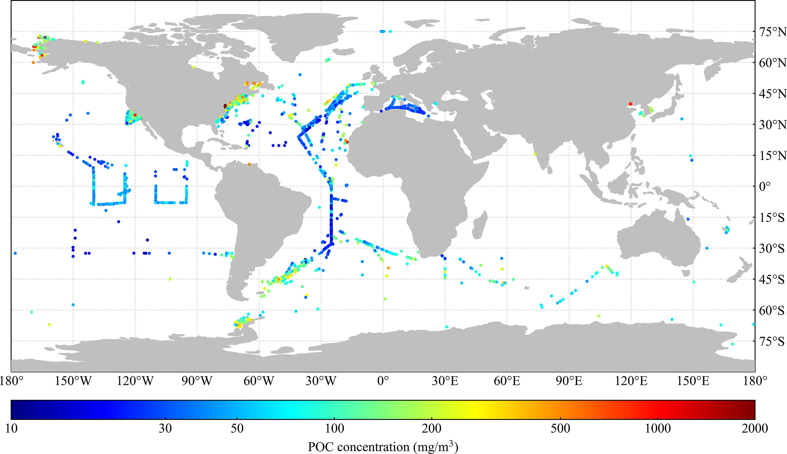
Figure 1 Geographical distribution of match-ups between the in situ dataset and satellite data. The color bar represents the average POC concentration (mg/m³) 10 m below the water surface.

FIGURE 2

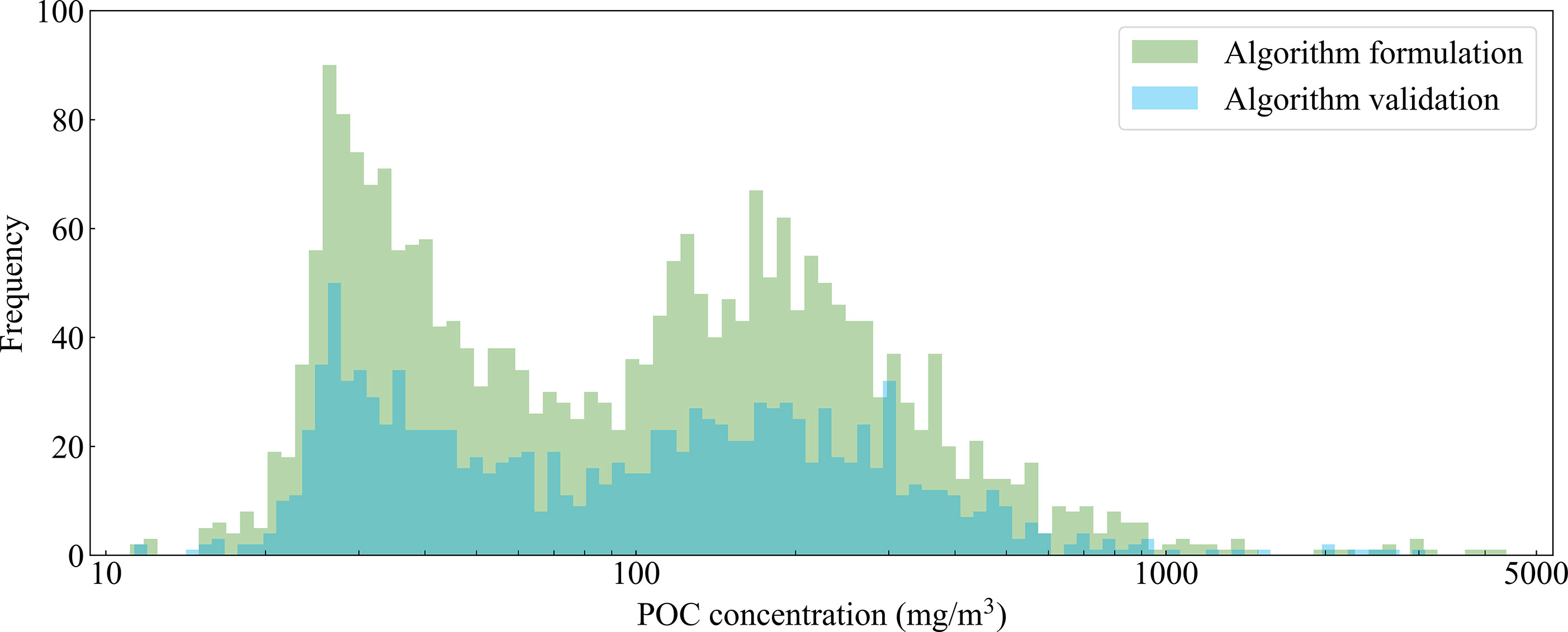
Figure 2 Histogram of POC concentration distribution for algorithm formulation match-ups and algorithm validation match-ups.

FIGURE 3

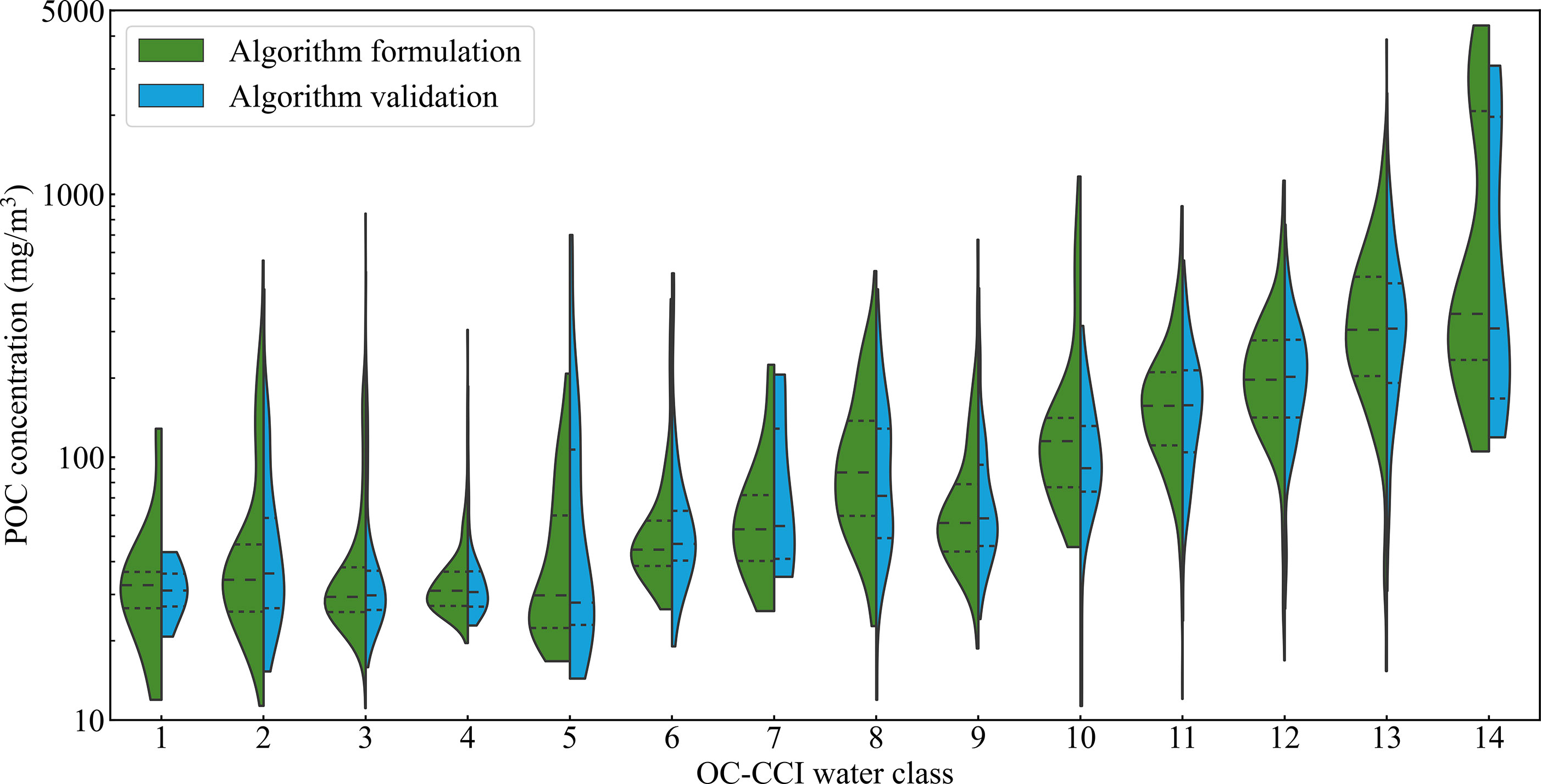
Figure 3 The distribution of OC-CCI dominant water classes corresponds to the match-ups. The height of the bulges on both sides indicates the density of the match-ups, and the black dashed lines represent the quartile lines.

2.4 Statistical metrics

In addition to the visual measurement of the product images generated by the a-POC algorithm, the performance of the algorithm was also evaluated by six statistical metrics:

● Pearson correlation coefficient between the measured value (x_i ) and the satellite-derived value (y_i ), R;

● Slope (S) and intercept (I) between x_i and y_i from Model-II linear regression (Reduced Major Axis);

● The median absolute percentage deviation (MAPD, %) between x_i and y_i , calculated as the median of the respective absolute percentage deviation, $\text{APD}=\frac{\left|{\text{y}}_{\text{i}}-{\text{x}}_{\text{i}}\right|}{{\text{x}}_{\text{i}}}\times 100$;

● Root-mean-square difference (RMSD, mg/m³) between x_i and y_i , $\text{RMSD}=\sqrt{\frac{1}{\text{N}}\sum ({\text{y}}_{\text{i}}-{\text{x}}_{\text{i}}{)}^2}$, where N is the number of match-ups used in the calculation;

● Bias between x_i and y_i , $\text{Bias}=\frac{1}{\text{N}}\sum \left({\text{y}}_{\text{i}}-{\text{x}}_{\text{i}}\right)$.

2.5 Formulation of a-POC algorithm

The relationship between the absorption coefficient and the POC concentration was established based on a(490). Figure 4 shows the cubic polynomial fit between the in situ POC concentration for algorithm formulation match-ups and the a(490) from the OC-CCI v5.0 product suite. The relationship between POC and a(490) in the a-POC algorithm is described as follows:

FIGURE 4

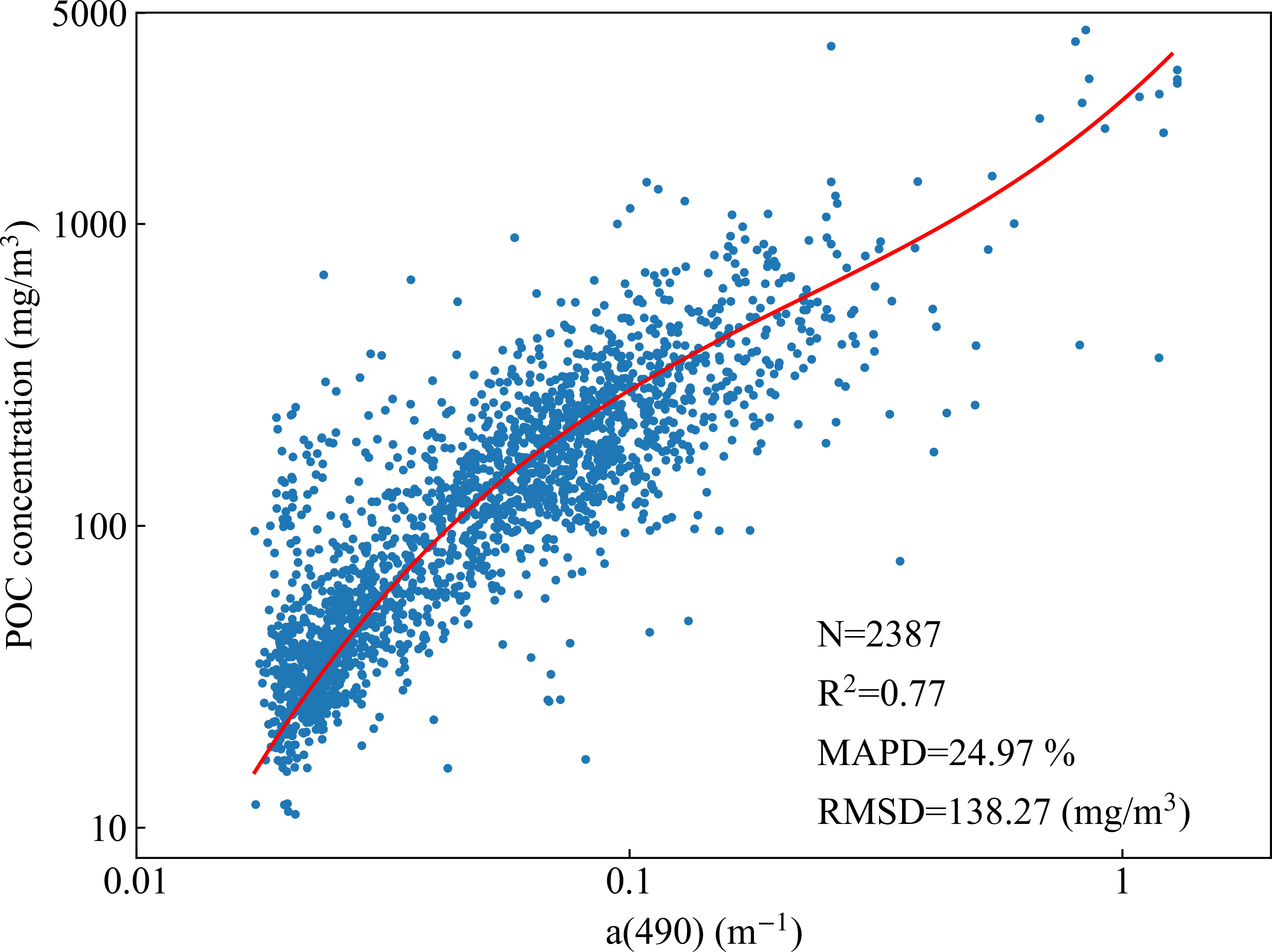
Figure 4 The relationship between the POC concentration and a(490) for algorithm formulation match-ups (N=2387) from the OC-CCI v5.0 product suite.

$\begin{array}{ll}\text{POC}={10}^{0.488{\text{x}}^3+0.947{\text{x}}^2+1.42\text{x}+3.41}& \text{,}\end{array}$

where x=log₁₀a(490) . The value for the squared correlation coefficient, R², between the POC concentration and a(490) obtained by cubic polynomial fitting was 0.77.

3 Results

3.1 Algorithm performance evaluation using algorithm validation match-ups

Figure 5 shows the frequency distribution of POC concentrations for algorithm validation match-ups and algorithm retrievals. The distribution of the algorithm validation match-ups showed a bimodal pattern, presenting at about 26 mg/m³ and 200 mg/m³. The a-POC algorithm underestimated the POC concentrations in the low-value interval, where the distribution clustered near 30 mg/m³. When the POC concentration was higher than 100 mg/m³, the a-POC algorithm roughly reproduced the histogram shape of the match-ups. For comparison, a similar evaluation was performed for the BG algorithm. The BG algorithm and a-POC algorithm had a similar histogram shape at the first peak, while the second peak significantly shifted to the left and was narrower than that of match-ups. In addition, the BG algorithm showed no frequency distribution when the POC concentration was higher than 800 mg/m³, indicating that the POC concentration estimated by the BG algorithm reached saturation.

FIGURE 5

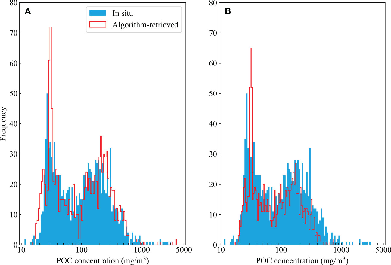
Figure 5 The frequency distribution of POC concentrations for algorithm validation match-ups and algorithm retrievals: (A) a-POC algorithm and (B) BG algorithm.

Statistical analysis was carried out, and the scatter plot and statistics metrics are shown in Figure 6 and Table 1, respectively. It can be seen that both a-POC and BG algorithms show significant correlations, with R² of 0.77 and 0.75 for a-POC and BG algorithms on the log₁₀ scale, respectively. The a-POC algorithm had a smaller error than the BG algorithm, with a Bias value of -3.29 mg/m³. The linear fitting line on the log₁₀ scale was closer to the 1:1 line, with a slope value of 0.91. However, the BG algorithm significantly underestimated the POC concentrations in the high-value range, with a Bias value of -49.06 mg/m³. The MAPD values ​​of the two algorithms were similar, and the RMSD were 128.49 and 184.48 mg/m³ for a-POC and BG algorithms, respectively. These results indicated that the a-POC algorithm was more suitable than the BG algorithm for retrieving POC concentrations, especially in regions with high POC concentrations (i.e., highly productive regions).

FIGURE 6

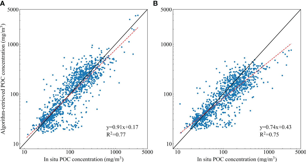
Figure 6 Correlation between in situ POC concentrations and the concentrations retrieved by (A) a-POC algorithm and (B) BG algorithm on the log₁₀ scale. The solid black line represents the 1: 1 line, and the red dashed line represents the corresponding linear regression line for each algorithm. The optimal linear regression equation (y) and the square of the determining coefficient (R²) on the log₁₀ scale are also presented.

TABLE 1

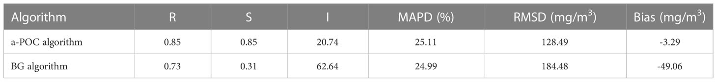
Table 1 Summary of statistical metrics characterizing the differences in POC concentration between the algorithm retrievals and values of algorithm validation match-ups.

3.2 Algorithm applied to OC-CCI data

3.2.1 Algorithm performance per OC-CCI water class

The performance of the a-POC algorithm is further evaluated to respond to the regional optimization of user groups and the calculation of per-pixel uncertainty. Figure 7 summarizes the statistical metrics of a-POC and BG algorithms per OC-CCI water class. Water classes 1-6 represent cleaner open oceans, and 12-14 represent coastal waters with high scattering characteristics. The algorithms performed differently in different water classes. When water classes were less than 13, both algorithms showed lower error levels, indicating that the algorithms perform similarly in open oceans and slightly turbid waters. The a-POC algorithm performed better in classes 13 and 14 (i.e., high turbid waters), especially in class 14, which represents the most optically complex waters. In contrast, the BG algorithm heavily underestimated POC concentrations in these classes.

FIGURE 7

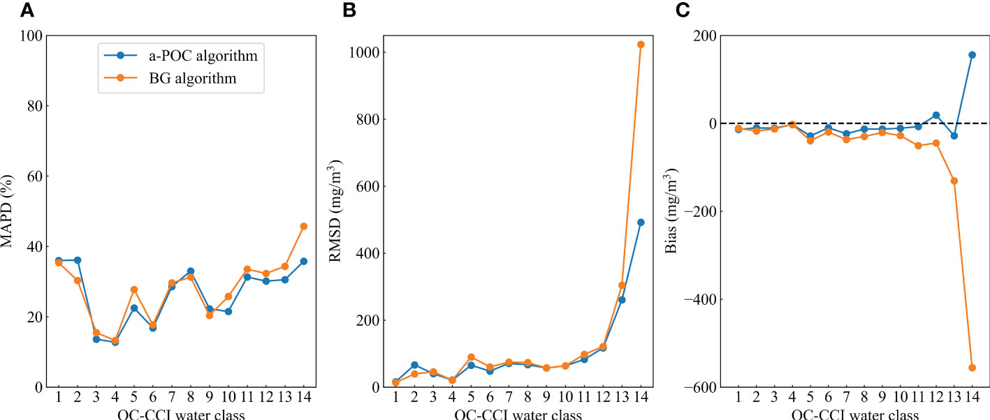
Figure 7 The statistical parameters of the algorithms per OC-CCI water class based on algorithm validation match-ups. (A) MAPD, (B) RMSD, and (C) Bias.

3.2.2 Algorithm applied in specific regions

In order to evaluate the applicability of the a-POC algorithm in waters with different turbidity degrees, in situ match-up datasets of the Atlantic Meridional Transect 26 (AMT26), CLIVEC-CV6, and the Chesapeake Bay were selected for algorithm validation. The AMT26 dataset was collected in September-October 2016 from the Atlantic oligotrophic gyre regions, with several match-ups (N=38) and POC concentrations ranging from 15.79 to 43.88 mg/m³ (Figures 8A, B). The CLIVEC-CV6 dataset was collected in June 2012 from the eastern coastal waters of the United States with typical coastal water characteristics (N=77), and the POC concentrations ranged from 109.83-635.25 mg/m³ (Figures 8D, E). The Chesapeake Bay belongs to highly turbid waters, and the Chesapeake Bay dataset was from the discover_aq_2011 cruise in July 2011, N=19, and the POC concentrations range was 1442.13-4389.28 mg/m³ (Figures 8G, H).

FIGURE 8

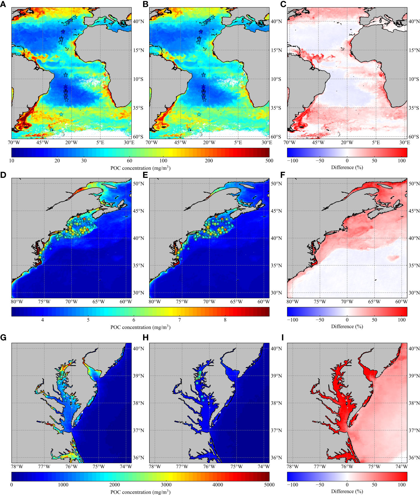
Figure 8 POC concentration distributions, including match-ups associated with (A–C) the Atlantic Meridional Transect 26 (AMT26), (D–F) the CLIVEC-CV6, and (G–I) the Chesapeake Bay datasets. The colors of scattered points correspond to the bottom color bar showing the POC concentrations of the match-ups. The background maps in (A, B) show the POC concentrations derived from a monthly average composite OC-CCI data in October 2016 using a-POC and BG algorithms, respectively. The patterns of panels (D, E) are similar to those of panels (A, B); background maps were derived in June 2012. The patterns of panels (G, H) are similar to those of panels (A, B); background maps were derived in July 2011. The percentage difference between the two algorithms is highlighted in (C, F, I), and the color pattern corresponds to the bottom color bar displaying the difference values. The percentage difference is calculated as 100×(POC_a−POC−POC_BG)/POC_BG.

The geographic and POC concentration distributions for match-ups of the AMT26, CLIVEC-CV6, and Chesapeake Bay datasets are shown in Figure 8. The background maps in panels (Figures 8A, D, G) and (Figures 8B, E, H) show POC concentrations derived from monthly average composite OC-CCI data associated with corresponding samples using a-POC and BG algorithms, respectively, and the percentage differences between the two algorithms are shown in panels (Figures 8C, F, I). Table 2 summarizes the statistical parameters between the POC concentrations retrieved by algorithms during the 1-day time window and the values of match-ups.

TABLE 2

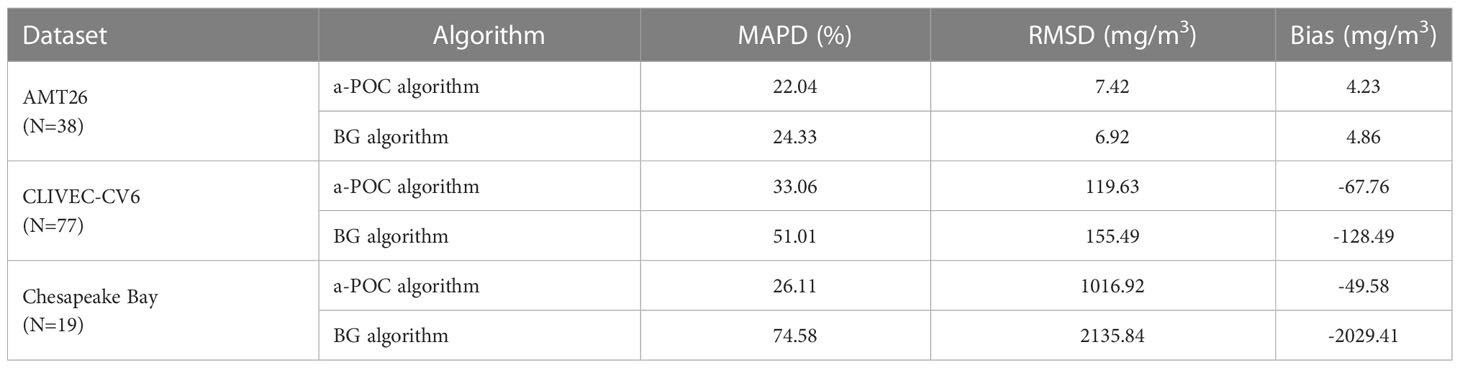
Table 2 The summary of statistical metrics characterizing the differences in POC concentration between algorithm retrievals and match-ups in specific regions.

For the AMT26 dataset, both algorithms reproduced the POC concentrations of match-ups and achieved similar results. The a-POC algorithm had lower MAPD and Bias values, but RMSD values were slightly higher than those of the BG algorithm due to the overestimation of the POC concentrations of individual match-ups. It can be seen from the background maps of Figure 8 that the POC concentrations retrieved by the algorithms had high consistency in the oligotrophic gyre regions. For the CLIVEC-CV6 dataset, the statistical metrics of the a-POC algorithm outperformed those of the BG algorithm. In addition, both algorithms underestimated POC concentrations, with Bias values of -67.76 and -128.49 mg/m³, respectively. This result is also evidenced by the monthly average products in Figure 8, where the two algorithms had a significant percentage difference in the regions close to the shore.

Compared to AMT26 and CLIVEC-CV6, these two algorithms produced considerable differences between retrieved POC concentrations and the values of match-ups in the Chesapeake Bay. The a-POC algorithm showed significant advantages, with RMSD and Bias values ​​of 1016.92 and -49.58 mg/m³, respectively. However, the RMSD and Bias values for the BG algorithm ​​were 2135.84 and -2029.41mg/m³, respectively, and POC concentrations did not exceed 800mg/m³, severely underestimated POC concentrations. Figure 8H shows that the BG algorithm saturated POC concentrations in the Chesapeake Bay, making the two algorithms produce a significant percentage difference of more than 100%.

Overall, the a-POC algorithm produced satisfactory results in open oceans, coastal waters, and highly turbid waters, with MAPD values ​​of 22.04, 33.06, and 26.11%, respectively. It outperformed the BG algorithm, especially in coastal waters and highly turbid waters.

3.2.3 Algorithm applied in global surface ocean

We further assessed the performance of the a-POC algorithm at the macroscopic scale and compared it with the BG algorithm. Panels (A) and (B) in Figure 9 show the global POC concentration distribution generated by applying a-POC and BG algorithms to the OC-CCI monthly average composite data in March 2020, respectively. Both algorithms produced similar patterns of concentration change in most open oceans. In the equatorial Atlantic and Pacific Oceans, seawater is blown away on both sides of the equator due to the influence of easterly trade winds (Gill and Adrian, 1982). The divergence of surface ocean currents causes an upwelling of cold and nutrient-rich waters, producing productive phytoplankton bloom zones and leading to higher POC concentrations than in subtropical gyre regions (Liu and Wang, 2022). At high latitudes, ocean surface waters are cold with a slight vertical density gradient. The vertical mixing depth of the water is much greater than the depth of the euphotic layer (Siegel et al., 2002). Due to vertical mixing, there is an abundant supply of nutrients in the South Ocean, North Atlantic, and North Pacific, resulting in higher POC concentrations. The a-POC algorithm more precisely captured the spatial characteristics of high POC concentrations. In coastal waters, the a-POC algorithm produced higher POC concentrations than the BG algorithm.

FIGURE 9

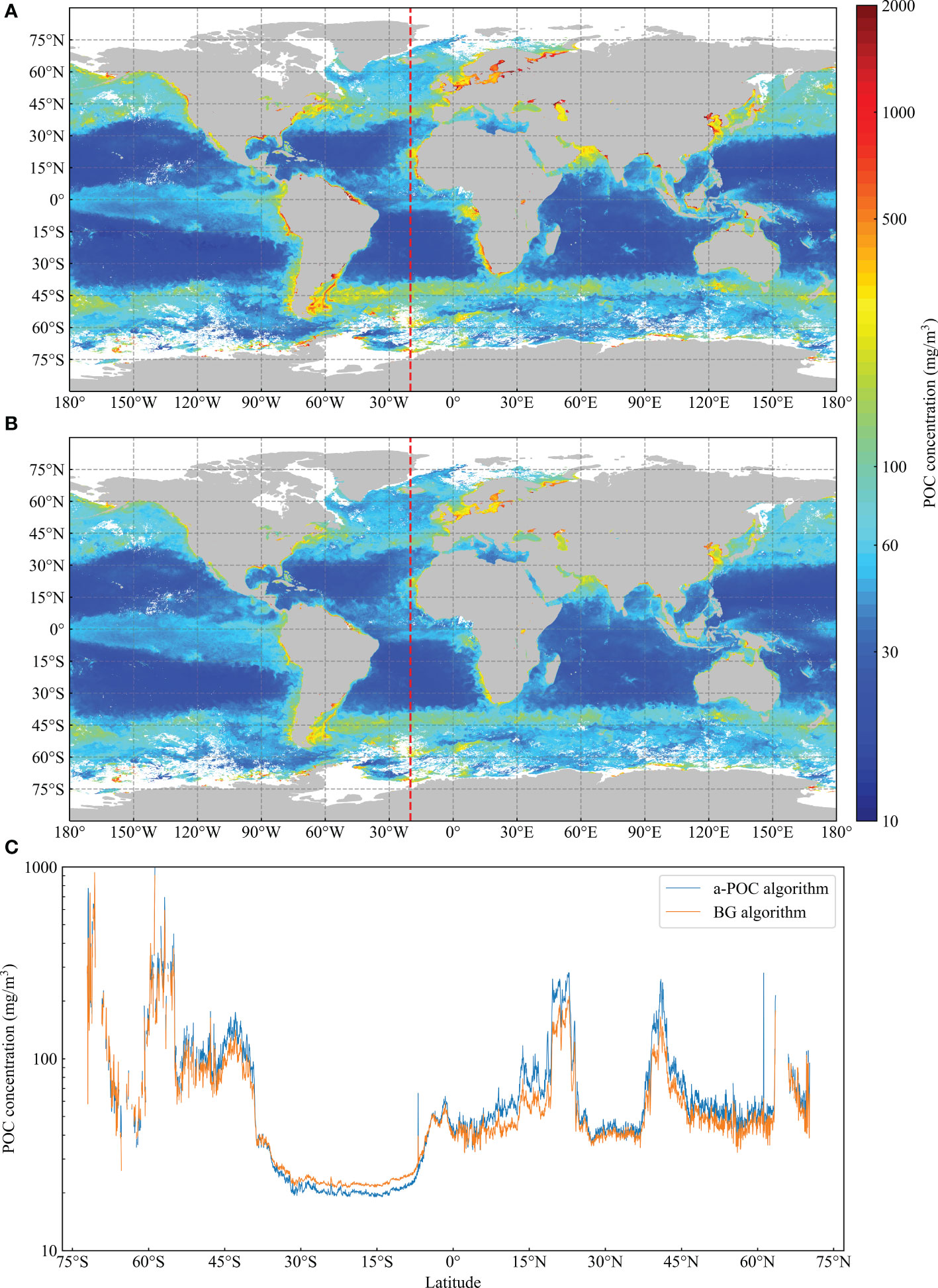
Figure 9 POC concentration distribution retrieved by (A) the a-POC algorithm and (B) the BG algorithm applied to monthly average composite OC-CCI data in March 2020, and (C) the POC concentration distribution along the 20°W transect through the Atlantic Ocean.

As shown in Figure 9C, the POC concentrations retrieved by the two algorithms were extracted along a transect through the Atlantic Ocean at 20°W, and the POC concentration change was generated with latitude as the independent variable. The trend was consistent for both algorithms, with retrieved POC concentrations ranging from 10 to 1000 mg/m³. The a-POC algorithm retrieved lower POC concentrations than the BG algorithm in the South Atlantic, consistent with the validation results of the AMT26 dataset. In the northwestern coastal region of Africa at 15-30°N, the a-POC algorithm showed reasonably higher POC concentrations, which can be demonstrated by the validation results in the coastal waters of the United States.

Precise POC concentration mapping in the global surface ocean can be used to estimate total pools of POC in the mixed layer, providing an insight into the global ocean carbon cycle. After considering seasonal and regional variations and assuming homogeneity of the mixed layer, the two algorithms were applied to all monthly average composite OC-CCI data in 2020. Afterward, the obtained POC concentrations were integrated over the mixed-layer depth. The mixed-layer depth data were derived from MIMOC (https://www.pmel.noaa.gov/mimoc/) (Schmidtko et al., 2013). The average total pools of POC estimated by a-POC and BG algorithms were 1.00 Pg C and 0.87 Pg C, respectively. The above evaluations indicated that the a-POC algorithm was robust in both open oceans and coastal waters compared with the BG algorithm. Thus, the total pool estimated by the a-POC algorithm was more credible.

3.3 Mapped uncertainties

Based on the performance of algorithms per OC-CCI water class in Section 3.2.1, the uncertainties of algorithms in the global surface ocean were mapped without in situ dataset distribution. The uncertainty of each pixel is obtained by calculating a weighted average based on each water class percent membership and then multiplying it with the statistical parameters of the corresponding water class. Supplementary Figure 1 shows the distribution of the OC-CCI dominant water class in the global ocean in March 2020. From the open ocean to the mainland, there was an increasing trend of water classes, with classes 13 and 14 concentrated along the coasts of the northern hemisphere.

The calculation procedure for uncertainties was applied to the data in Figure 9 to obtain the statistical metric distribution of algorithms (Figure 10). In general, the trend of statistical metric distribution was consistent with the match-up validation results. Both algorithms performed similarly in open oceans (i.e., lower water classes), with lower MAPD, RMSD, and Bias values for the a-POC algorithm. As expected, the two algorithms showed significant differences in the southern Atlantic, the Baltic Sea, and the Yellow and Bohai Seas in China, where corresponding OC-CCI water classes were high. In these regions, the a-POC algorithm slightly overestimated POC concentrations, while the BG algorithm underestimated POC concentrations with poor statistical metrics.

FIGURE 10

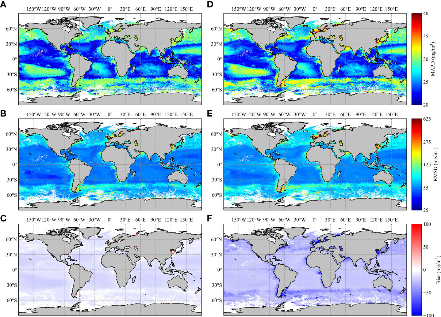
Figure 10 Distribution of statistical metrics MAPD, RMSD, and Bias associated with OC-CCI water class when (A–C) a-POC algorithm and (D–F) BG algorithm are applied to the monthly average OC-CCI data in March 2020.

4 Discussion

4.1 Algorithm applied to OLCI data in Bohai Sea of China

The a-POC algorithm showed significant advantages over BG algorithms when applied to OC-CCI v5.0 data, and user groups may want to apply a-POC algorithms to specific ocean color sensors. To evaluate the universality of the a-POC algorithm to specific ocean color sensors and the sensitivity to different atmospheric correction algorithms, the a-POC and BG algorithms were applied OLCI data associated with the Bohai Sea dataset (Figure 11). The POC concentrations in the Bohai Sea dataset ranged from 338.0 to 1380.0 mg/m³. The OLCI data were pre-processed by the BAC algorithm (Moore et al., 1999) and the POLYMER algorithm (Steinmetz et al., 2011). After the OLCI data pre-processing and match-up procedure, 23 match-ups were obtained for the BAC algorithm and 28 for the POLYMER algorithm, and the in situ sampling dates were June 14, September 19, and 23, 2017. As expected, the BAC algorithm has stricter quality flags than the POLYMER algorithm (Mograne et al., 2019; Renosh et al., 2020). The BAC algorithm reduced the match-ups by 5 due to the influence of the atmospheric correction failure flag. Figure 12 shows the scatter plots of in situ R_rs(λ) versus OLCI-derived R_rs(λ) at 443 nm, 490 nm, 560 nm, and 665 nm using the atmospheric correction algorithms. These bands were used by the QAA_V5 and BG algorithms to obtain the absorption coefficients and POC concentrations, respectively. The two atmospheric correction algorithms differed significantly at 443 nm. The R_rs(443) obtained by the BAC algorithm were significantly underestimated and discrete, while those obtained by the POLYMER algorithm were more consistent with the in situ R_rs(443). In other bands, both algorithms had similar performances at other bands.

FIGURE 11

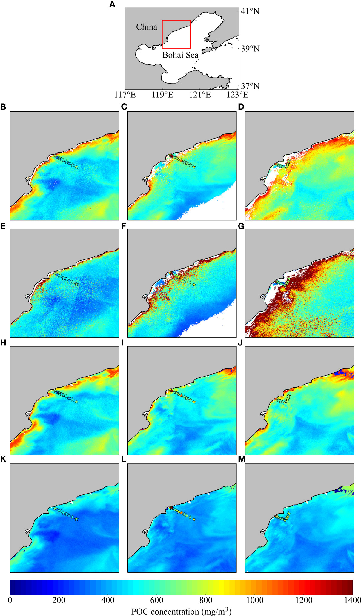
Figure 11 Distribution of POC associated with the Bohai Sea match-ups dataset. (A) The geographical location of the Bohai Sea. The red box corresponds to the range of the panels below. The color of scatters and background map in (B–M) corresponds to the bottom color bar representing the POC concentration. The background maps in (B–G) are POC concentrations retrieved by the (B–D) a-POC algorithm and (E–G) BG algorithm. These data are from OLCI data pre-processed by the BAC atmospheric correction algorithm on June 14, September 19, and 23, 2017. Panels (H–M) used the same date and color patterns as panels (B–G), OLCI data were pre-processed by the POLYMER atmospheric correction algorithm, and POC concentrations were retrieved by the (H–J) a-POC algorithm and (K–M) BG algorithm.

FIGURE 12

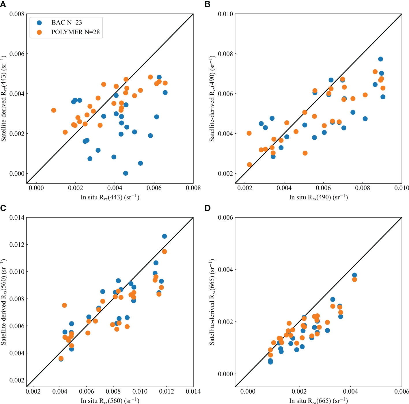
Figure 12 Scatter plots of OLCI remote sensing reflectance (R_rs(λ)) derived by the BAC algorithm and POLYMER algorithm with match-up R_rs(λ) at (A) 443 nm, (B) 490 nm, (C) 560 nm, and (D) 665 nm. The solid black line represents the 1:1 line.

Figure 11 found that the scatters were closer to the color of the background maps generated by the a-POC algorithm, i.e., the POC concentrations retrieved by the a-POC algorithm were closer to that of the match-ups. Furthermore, different atmospheric correction algorithms significantly impact the estimation of POC concentrations, which was especially true for the BG algorithm (Figures 11E–G). When the BG algorithm was applied to OLCI data pre-processed by the BAC algorithm, a large amount of noise was generated, and the estimated POC concentrations were seriously inconsistent with the match-ups. Because the BG algorithm relies too much on the accuracy of R_rs(443), the strong absorption of CDOM and debris at 443 nm prevents the accurate identification of aerosol models from LUTs by the BAC algorithm, leading to a significant underestimation of R_rs(443) (Li et al., 2022). Therefore, an accurate atmospheric correction is essential for the BG algorithm. In contrast, the atmospheric correction has less impact on the a-POC algorithm because the QAA algorithm weakens the dominance of R_rs(443) in the calculation of absorption coefficients (Lee et al., 2002; Lee et al., 2009). For the OLCI data pre-processed by the POLYMER algorithm, the quality of the POC concentration distribution maps generated by both algorithms was significantly improved. Compared with the match-ups, the BG algorithm significantly underestimated POC concentrations (Figures 11H–M).

The statistical parameters between POC algorithms and match-ups are summarized in Table 3. Consistent with the image analysis, the POC concentrations were all overestimated to varying degrees when the POC algorithms were applied to the OLCI data pre-processed by the BAC algorithm. The Bias values for the a-POC and BG algorithms were 16.80 mg/m³ and 741.83mg/m³, respectively. In contrast, when the POC algorithms were applied to the OLCI data pre-processed by the POLYMER algorithm, both algorithms underestimated the POC concentrations, and Bias values were -89.04 mg/m³ and -297.83mg/m³, respectively. After applying the POC algorithms to the OLCI data pre-processed by the BAC and POLYMER algorithms, the RMSD value for the BG algorithm plummeted from 396.94 mg/m³ to 66.26 mg/m³. This result was contrary to the trend of MAPD because the noise generated by the BAC algorithm partially offsets the underestimation of POC concentrations retrieved by the BG algorithm. In comparison, the RMSD value of the a-POC algorithm decreased from 40.08 mg/m³ to 35.97 mg/m³, indicating that the a-POC algorithm was less sensitive to atmospheric correction than the BG algorithm. As expected, the BG algorithm was established solely based on in situ measurement data, making it a typical “in-water” algorithm. The accuracy of the BG algorithm is limited by the accuracy of the atmospheric correction algorithm (Hu et al., 2012; Le et al., 2018).

TABLE 3

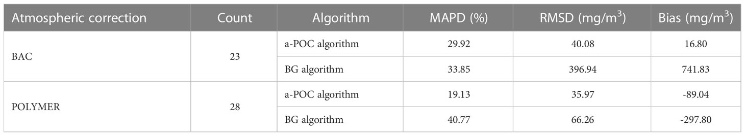
Table 3 Statistical metrics between POC concentrations in the Bohai Sea match-up dataset and algorithm retrievals applied to OLCI data pre-processed by different atmospheric correction algorithms.

Because the Bohai Sea is surrounded by land on three sides, the water optical environment is more complex, and the water class is dominated by classes 13 and 14 (Supplementary Figure 1). It strongly demonstrates the results of Section 3.2 that the a-POC algorithm was more suitable for retrieving the POC concentrations in high turbid waters than the BG algorithm.

4.2 Influence of the IOPs on the POC concentration retrieval

The complexity of POC composition indicates that accurate retrieval of POC remains a great challenge. For example, changes in the species composition of the phytoplankton community or the contribution of phytoplankton and non-phytoplankton particles to the total POC can change the optical properties of the seawater (Grob et al., 2007; Ras et al., 2008). In addition, some non-POC components, such as air bubbles and mineral particles, can also cause changes in the optical environment of the water column, affecting the accurate acquisition of scattering of organic particulate matter (Tassan and Ferrari, 1995; Stramski and Tegowski, 2001). These variations cause changes in the relationship between b_bp and POC, introducing uncertainty in estimating the POC concentration of b_bp. Based on an in situ measurement dataset, Gardner et al., 2006 found a robust relationship between c_p and POC. However, satellite remote sensing retrieval of c_p is difficult because c_p is the sum of particulate absorption and total particulate scattering. Total particle scattering is dominated by forward scattering, to which R_rs is theoretically insensitive (Evers-King et al., 2017; Le et al., 2018). Although machine-learning methods are robust in retrieval studies of global ocean surface POC concentrations (Liu et al., 2021), a better understanding of the relationship between particle properties and IOPs can improve POC algorithms by providing insight into the composition of the total POC pool (Evers-King et al., 2017).

When b_bp and c_p in IOPs were verified and limited, scholars started focusing on absorption coefficients. Stramski et al., 2001 have demonstrated that organic particles contribute more to the absorption coefficient than the backscattering coefficient, especially for the phytoplankton community, which is the main contribution to the optical variability in open oceans. For high productivity waters, Woźniak et al. (2010) indicated that the variation range of POC-specific particulate absorption coefficients spans one order of magnitude, while the variation of particulate scattering spans two orders of magnitude, suggesting that the POC-specific absorption coefficients are more constrained.

The successful application of the BG algorithm in open oceans demonstrates that the absorption coefficient is a meaningful optical proxy for the POC. The variation of R_rs(443) and R_rs(560) used by the BG algorithm is mainly driven by the variation of the absorption coefficient (Stramski et al., 2008). Unlike in open oceans, the mineral particles and CDOM in coastal waters mainly contribute to optical properties. The absorption at the short blue bands (i.e., 412 nm and 443 nm) is strongly influenced by a_CDOM, which is one of the reasons for the poor performance of the BG algorithm in these waters (Le et al., 2018). In addition, the size and scope of in situ datasets used to build the empirical algorithm also impact the accuracy of the BG algorithm (Siegel et al., 2005; Evers-King et al., 2017).

In this study, a(490) was selected as a proxy for POC concentration. First, all types of particles (mineral-dominated, organic-dominated, and mixed) have stronger absorption in the longer blue and shorter green wavelengths range (Allison et al., 2010; Woźniak et al., 2010), especially around 500 nm (see Figure 4 in Woźniak et al., 2010). We tried to use both a(490) and a(510) as proxies for POC and establish the relationship. Compared with a(490), the variation of a(510) was more constrained, thus amplifying the error when retrieving the POC concentration despite the similar fitting performance. Second, selecting a(490) as a proxy can reduce the effects of absorption by CDOM, especially in coastal waters (Le et al., 2017; Le et al., 2018). The direct use of a (490) obtained from the QAA algorithm reduces the error introduced by using R_rs in a single band as a proxy for the absorption coefficient. Despite the extensive spatial and larger concentration distribution range of the in situ dataset used to develop the a-POC algorithm, the POC concentrations were slightly overestimated in open oceans while underestimated in highly productive waters. Errors may occur as all the empirical algorithms were established based on certain assumptions (Hu et al., 2012). The a-POC algorithm assumes that a_CDOM and absorption of nonalgal inorganic particles in seawater are covariant with the absorption of organic particulate matter. As a result, the a-POC algorithm misestimates the contribution of non-POC sources to the absorption coefficient. Due to the absence of optical property data in the in situ POC dataset, the a-POC algorithm is not an “in-water” algorithm. It cannot show the actual physical relationship between the absorption coefficient and the POC concentration. In addition, the in situ dataset used in this study was derived from multiple cruises over a long period. The measurement method of POC concentration was difficult to standardize, creating uncertainty in the development of the a-POC algorithm. However, compared to “in-water” algorithms, the a-POC algorithm considers the partial errors introduced by atmospheric correction and the QAA algorithm, which helps the end-user to use the algorithm directly and to obtain higher accuracy.

5 Conclusions

In this study, a large in situ POC dataset was merged, which spans an extensive time and space and accurately captures the changing characteristics of seawater optical properties. The a-POC algorithm was formulated based on the in situ dataset. Compared with the BG algorithm, the application of the a-POC algorithm to the OC-CCI data improved the accuracy of POC concentration retrieval, especially in medium and high productivity waters. This improvement can be attributed to the robust relationship between the absorption coefficient at 490 nm from the OC-CCI v5.0 product suite and POC. As a result, the long-time series variation of POC concentrations in the global surface ocean was supported, and the estimation of total pools of POC in the mixed layer was promoted. Furthermore, the a-POC algorithm was also suitable for OLCI data, producing reliable results in the Bohai Sea of China. The a-POC algorithm was less sensitive to the influence of atmospheric correction algorithms, which was associated with low dependence on a single band when calculating the absorption coefficient using the QAA method. The a-POC algorithm was established based on the in situ POC dataset and the absorption coefficient of remote sensing data, which considered the uncertainty in the generation of remote sensing data. Therefore, when applying the a-POC algorithm to the original remote sensing data processed by different methods, the parameters of the algorithm need to be adjusted to reduce the error. In future field surveys, both the optical properties of seawater and biochemical parameters should be included in the measurement task, facilitating the verification of the genuine physical relationship between the absorption coefficient and the POC.

Data availability statement

Publicly available datasets were analyzed in this study. This data can be found here: https://seabass.gsfc.nasa.gov, https://datadryad.org/.

Author contributions

QL: All the calculations, preparation of figures, collation of the in situ database, and original draft preparation. LJ: Project administration, funding acquisition, review and editing, and investigation. YC: Project administration and collation of the in situ dataset in the Bohai Sea. JT: review and editing, methodology. SG: software and calculation code. All authors contributed to the article and approved the submitted version.

Funding

This work was supported by the<National Natural Science Foundation of China> under Grant (No. 42076186).

Acknowledgments

We would like to thank the Remote Sensing Group of the National Marine Environmental Monitoring Centre of China for providing partial in situ datasets. We would like to thank the scientists who contributed in situ data to the shared database for our use. We would like to thank the ESA climate office for providing the OC-CCI data. We would like to thank two reviewers for their thoughtful comments, which have helped us to improve this manuscript considerably.

Conflict of interest

The authors declare that the research was conducted in the absence of any commercial or financial relationships that could be construed as a potential conflict of interest.

Publisher’s note

All claims expressed in this article are solely those of the authors and do not necessarily represent those of their affiliated organizations, or those of the publisher, the editors and the reviewers. Any product that may be evaluated in this article, or claim that may be made by its manufacturer, is not guaranteed or endorsed by the publisher.

Supplementary material

The Supplementary Material for this article can be found online at: https://www.frontiersin.org/articles/10.3389/fmars.2022.1048893/full#supplementary-material

References

Allison D. B., Stramski D., Mitchell B. G. (2010). Empirical ocean color algorithms for estimating particulate organic carbon in the southern ocean. J. Geophysical Res: Oceans 115 (C10). doi: 10.1029/2009JC006040

CrossRef Full Text | Google Scholar

Amon R. M. W., Benner R. (1996). Bacterial utilization of different size classes of dissolved organic matter. Limnology Oceanography 41 (1), 41–51. doi: 10.4319/lo.1996.41.1.0041

CrossRef Full Text | Google Scholar

Babin M., Stramski D., Ferrari G. M., Claustre H., Bricaud A., Obolensky G., et al. (2003). Variations in the light absorption coefficients of phytoplankton, nonalgal particles, and dissolved organic matter in coastal waters around Europe. J. Geophysical Res.: Oceans 108, C7. doi: 10.1029/2001JC000882

CrossRef Full Text | Google Scholar

Behrenfeld M. J., Boss E., Siegel D. A., Shea D. M. (2005). Carbon-based ocean productivity and phytoplankton physiology from space. Global Biogeochemical Cycles 19 (1). doi: 10.1029/2004GB002299

CrossRef Full Text | Google Scholar

Bishop J. K. B. (1999). Transmissometer measurement of POC. Deep Sea Res. Part I: Oceanographic Res. Papers 46 (2), 353–369. doi: 10.1016/S0967-0637(98)00069-7

CrossRef Full Text | Google Scholar

Cetinić I., Perry M. J., Briggs N. T., Kallin E., D'Asaro E. A., Lee C. M. (2012). Particulate organic carbon and inherent optical properties during 2008 north Atlantic bloom experiment. J. Geophysical Res: Oceans 117 (C6). doi: 10.1029/2011JC007771

CrossRef Full Text | Google Scholar

Chen D., Zeng L., Boot K., Liu Q. (2022). Satellite observed spatial and temporal variabilities of particulate organic carbon in the East China Sea. Remote Sens. 14 (8), 1799. doi: 10.3390/rs14081799

CrossRef Full Text | Google Scholar

Cui T., Zhang J., Groom S., Sun L., Smyth T., Sathyendranath S. (2010). Validation of MERIS ocean-color products in the bohai Sea: A case study for turbid coastal waters. Remote Sens. Environ. 114 (10), 2326–2336. doi: 10.1016/j.rse.2010.05.009

CrossRef Full Text | Google Scholar

Duan H., Feng L., Ma R., Zhang Y., Arthur Loiselle S. (2014). Variability of particulate organic carbon in inland waters observed from MODIS aqua imagery. Environ. Res. Lett. 9 (8), 84011. doi: 10.1088/1748-9326/9/8/084011

CrossRef Full Text | Google Scholar

Duforêt-Gaurier L., Loisel H., Dessailly D., Nordkvist K., Alvain S. (2010). Estimates of particulate organic carbon over the euphotic depth from in situ measurements. application to satellite data over the global ocean. Deep Sea Res. Part I: Oceanographic Res. Papers 57 (3), 351–367. doi: 10.1016/j.dsr.2009.12.007

CrossRef Full Text | Google Scholar

Evers-King H., Martinez-Vicente V., Brewin R. J., Dall'Olmo G., Hickman A. E., Jackson T., et al. (2017). Validation and intercomparison of ocean color algorithms for estimating particulate organic carbon in the oceans. Front. Mar. Sci. 4. doi: 10.3389/fmars.2017.00251

CrossRef Full Text | Google Scholar

Field Christopher B., Behrenfeld Michael J., Randerson James T., Falkowski P. (1998). Primary production of the biosphere: Integrating terrestrial and oceanic components. Science 281 (5374), 237–240. doi: 10.1126/science.281.5374.237

PubMed Abstract | CrossRef Full Text | Google Scholar

Gardner W. D., Mishonov A. V., Richardson M. J. (2006). Global POC concentrations from in-situ and satellite data. Deep Sea Res. Part II: Topical Stud. Oceanography 53 (5), 718–740. doi: 10.1016/j.dsr2.2006.01.029

CrossRef Full Text | Google Scholar

Gardner W. D., Richardson M. J., Carlson C. A., Hansell D., Mishonov A. V. (2003). Determining true particulate organic carbon: bottles, pumps and methodologies. Deep Sea Res. Part II: Topical Stud. Oceanography 50 (3), 655–674. doi: 10.1016/S0967-0645(02)00589-1

CrossRef Full Text | Google Scholar

Gill A. E., Adrian E. (1982). Atmosphere-ocean dynamics (New York:Academic press).

Google Scholar

Gordon H. R., Wang M. (1994a). Influence of oceanic whitecaps on atmospheric correction of ocean-color sensors. Appl. Optics 33 (33), 7754–7763. doi: 10.1364/AO.33.007754

CrossRef Full Text | Google Scholar

Gordon H. R., Wang M. (1994b). Retrieval of water-leaving radiance and aerosol optical thickness over the oceans with SeaWiFS: a preliminary algorithm. Appl. Optics 33 (3), 443–452. doi: 10.1364/AO.33.000443

CrossRef Full Text | Google Scholar

Grob C., Ulloa O., Claustre H., Huot Y., Alarcón G., Marie D. (2007). Contribution of picoplankton to the total particulate organic carbon concentration in the eastern south pacific. Biogeosciences 4 (5), 837–852. doi: 10.5194/bg-4-837-2007

CrossRef Full Text | Google Scholar

Hedges J. I. (1992). Global biogeochemical cycles: progress and problems. Mar. Chem. 39 (1), 67–93. doi: 10.1016/0304-4203(92)90096-S

CrossRef Full Text | Google Scholar

Hedges J. I., Stern J. H. (1984). Carbon and nitrogen determinations of carbonate-containing solids1. Limnology Oceanography 29 (3), 657–663. doi: 10.4319/lo.1984.29.3.0657

CrossRef Full Text | Google Scholar

Hu C., Lee Z., Franz B. (2012). Chlorophyll aalgorithms for oligotrophic oceans: A novel approach based on three-band reflectance difference. J. Geophysical Research: Oceans 117 (C1). doi: 10.1029/2011JC007395

CrossRef Full Text | Google Scholar

Jackson T., Sathyendranath S., Mélin F. (2017). An improved optical classification scheme for the ocean colour essential climate variable and its applications. Remote Sens. Environ. 203, 152–161. doi: 10.1016/j.rse.2017.03.036

CrossRef Full Text | Google Scholar

Jahnke R. A. (1996). The global ocean flux of particulate organic carbon: Areal distribution and magnitude. Global Biogeochemical Cycles 10 (1), 71–88. doi: 10.1029/95GB03525

CrossRef Full Text | Google Scholar

Jiang L., Guo X., Wang L., Sathyendranath S., Evers-King H., Chen Y., et al. (2020). Validation of MODIS ocean-colour products in the coastal waters of the yellow Sea and East China Sea. Acta Oceanologica Sin. 39 (1), 91–101. doi: 10.1007/s13131-019-1522-3

CrossRef Full Text | Google Scholar

Jiang G., Loiselle S. A., Yang D., Gao C., Ma R., Su W., et al. (2019). An absorption-specific approach to examining dynamics of particulate organic carbon from VIIRS observations in inland and coastal waters. Remote Sens. Environ. 224, 29–43. doi: 10.1016/j.rse.2019.01.032

CrossRef Full Text | Google Scholar

Lee Z., Carder K. L., Arnone R. A. (2002). Deriving inherent optical properties from water color: a multiband quasi-analytical algorithm for optically deep waters. Appl. Optics 41 (27), 5755–5772. doi: 10.1364/AO.41.005755

CrossRef Full Text | Google Scholar

Lee Z., Lubac B., Werdell J., Arnone R. (2009). “An update of the quasi-analytical algorithm (QAA_v5),” in International ocean color group software report.

Google Scholar

Le C., Lehrter J. C., Hu C., MacIntyre H., Beck M. W. (2017). Satellite observation of particulate organic carbon dynamics on the Louisiana continental shelf. J. Geophysical Research: Oceans 122 (1), 555–569. doi: 10.1002/2016JC012275

CrossRef Full Text | Google Scholar

Le C., Zhou X., Hu C., Lee Z., Li L., Stramski D. (2018). A color-index-based empirical algorithm for determining particulate organic carbon concentration in the ocean from satellite observations. J. Geophysical Research: Oceans 123 (10), 7407–7419. doi: 10.1029/2018JC014014

CrossRef Full Text | Google Scholar

Li Q., Jiang L., Chen Y., Wang L., Wang L. (2022). Evaluation of seven atmospheric correction algorithms for OLCI images over the coastal waters of qinhuangdao in bohai Sea. Regional Stud. Mar. Sci. 56, 102711. doi: 10.1016/j.rsma.2022.102711

CrossRef Full Text | Google Scholar

Lin J., Lyu H., Miao S., Pan Y., Wu Z., Li Y., et al. (2018). A two-step approach to mapping particulate organic carbon (POC) in inland water using OLCI images. Ecol. Indic. 90, 502–512. doi: 10.1016/j.ecolind.2018.03.044

CrossRef Full Text | Google Scholar

Liu D., Bai Y., He X. Q., Tao B. Y., Pan D. L., Chen C. T. A., et al. (2019). Satellite estimation of particulate organic carbon flux from changjiang river to the estuary. Remote Sens. Environ. 223, 307–319. doi: 10.1016/j.rse.2019.01.025

CrossRef Full Text | Google Scholar

Liu H., Li Q., Bai Y., Yang C., Wang J., Zhou Q., et al. (2021). Improving satellite retrieval of oceanic particulate organic carbon concentrations using machine learning methods. Remote Sens. Environ. 256, 112316. doi: 10.1016/j.rse.2021.112316

CrossRef Full Text | Google Scholar

Liu X., Wang M. (2022). Global daily gap-free ocean color products from multi-satellite measurements. Int. J. Appl. Earth Observation Geoinformation 108, 102714. doi: 10.1016/j.jag.2022.102714

CrossRef Full Text | Google Scholar

Loisel H., Nicolas J.-M., Deschamps P.-Y., Frouin R. (2002). Seasonal and inter-annual variability of particulate organic matter in the global ocean. Geophysical Res. Lett. 29 (24), 49–41-49-44. doi: 10.1029/2002GL015948

CrossRef Full Text | Google Scholar

Martiny A. C., Vrugt J. A., Lomas M. W. (2014). Concentrations and ratios of particulate organic carbon, nitrogen, and phosphorus in the global ocean. Sci. Data 1 (1), 140048. doi: 10.1038/sdata.2014.48

PubMed Abstract | CrossRef Full Text | Google Scholar

Mélin F., Sclep G. (2015). Band shifting for ocean color multi-spectral reflectance data. Optics Express 23 (3), 2262–2279. doi: 10.1364/OE.23.002262

PubMed Abstract | CrossRef Full Text | Google Scholar

Mograne M., Jamet C., Loisel H., Vantrepotte V., Mériaux X., Cauvin A., et al (2019). Evaluation of five atmospheric correction algorithms over French optically-complex waters for the sentinel-3A OLCI ocean color sensor. Remote Sens. 11 (6), 668. doi: 10.3390/rs11060668

CrossRef Full Text | Google Scholar

Moore G. F., Aiken J., Lavender S. J. (1999). The atmospheric correction of water colour and the quantitative retrieval of suspended particulate matter in case II waters: Application to MERIS. Int. J. Remote Sens. 20 (9), 1713–1733. doi: 10.1080/014311699212434

CrossRef Full Text | Google Scholar

Moore T. S., Campbell J. W., Hui F. (2001). A fuzzy logic classification scheme for selecting and blending satellite ocean color algorithms. IEEE Trans. Geosci. Remote Sens. 39 (8), 1764–1776. doi: 10.1109/36.942555

CrossRef Full Text | Google Scholar

Mueller J. L., Morel A., Frouin R., Davis C., Arnone R., Carder K., et al. (2003). “Ocean optics protocols for satellite ocean color sensor validation, revision 4. volume III,” in Radiometric measurements and data analysis protocols (Greenbelt, MD: USA: Goddard Space Flight Space Center).

Google Scholar

Omand M. M., D’Asaro E. A., Lee C. M., Perry M. J., Briggs N., Cetinić I., et al. (2015). Eddy-driven subduction exports particulate organic carbon from the spring bloom. Science 348 (6231), 222–225. doi: 10.1126/science.1260062

PubMed Abstract | CrossRef Full Text | Google Scholar

Pabi S., Arrigo K. R. (2006). Satellite estimation of marine particulate organic carbon in waters dominated by different phytoplankton taxa. J. Geophysical Research: Oceans 111 (C9). doi: 10.1029/2005JC003137

CrossRef Full Text | Google Scholar

Ras J., Claustre H., Uitz J. (2008). Spatial variability of phytoplankton pigment distributions in the subtropical south pacific ocean: comparison between in situ and predicted data. Biogeosciences 5 (2), 353–369. doi: 10.5194/bg-5-353-2008

CrossRef Full Text | Google Scholar

Renosh P. R., Doxaran D., Keukelaere L. D., Gossn J. I. (2020). Evaluation of atmospheric correction algorithms for sentinel-2-MSI and sentinel-3-OLCI in highly turbid estuarine waters. Remote Sens. 12 (8), 1285. doi: 10.3390/rs12081285

CrossRef Full Text | Google Scholar

Sathyendranath S., Brewin R. J. W., Brockmann C., Brotas V., Calton B., Chuprin A., et al. (2019). An ocean-colour time series for use in climate studies: The experience of the ocean-colour climate change initiative (OC-CCI). Sensors 19 (19), 4285. doi: 10.3390/s19194285

PubMed Abstract | CrossRef Full Text | Google Scholar

Sathyendranath S. J. T., Brockmann C., Brotas V., Calton B., Chuprin A., Clements O., et al. (2021). ESA Ocean colour climate change initiative (Ocean_Colour_cci): Version 5.0 data. NERC EDS Centre Environ. Data Analysis. doi: 10.5285/1dbe7a109c0244aaad713e078fd3059a

CrossRef Full Text | Google Scholar

Schmidtko S., Johnson G. C., Lyman J. M. (2013). MIMOC: A global monthly isopycnal upper-ocean climatology with mixed layers. J. Geophysical Res: Oceans 118 (4), 1658–1672. doi: 10.1002/jgrc.20122

CrossRef Full Text | Google Scholar

Sharp J. H. (1974). Improved analysis for “particulate” organic carbon and nitrogen from seawater1. Limnology Oceanography 19 (6), 984–989. doi: 10.4319/lo.1974.19.6.0984

CrossRef Full Text | Google Scholar

Siegel D. A., Doney S. C., Yoder J. A. (2002). The north Atlantic spring phytoplankton bloom and sverdrup's critical depth hypothesis. Science 296 (5568), 730–733. doi: 10.1126/science.1069174

PubMed Abstract | CrossRef Full Text | Google Scholar

Siegel D. A., Maritorena S., Nelson N. B., Behrenfeld M. J., McClain C. R. (2005). Colored dissolved organic matter and its influence on the satellite-based characterization of the ocean biosphere. Geophysical Res. Lett. 32 (20). doi: 10.1029/2005GL024310

CrossRef Full Text | Google Scholar

Siegenthaler U., Sarmiento J. L. (1993). Atmospheric carbon dioxide and the ocean. Nature 365 (6442), 119–125. doi: 10.1038/365119a0

CrossRef Full Text | Google Scholar

Steinmetz F., Deschamps P.-Y., Ramon D. (2011). Atmospheric correction in presence of sun glint: application to MERIS. Optics Express 19 (10), 9783–9800. doi: 10.1364/OE.19.009783

PubMed Abstract | CrossRef Full Text | Google Scholar

Stramska M. (2009). Particulate organic carbon in the global ocean derived from SeaWiFS ocean color. Deep Sea Res. Part I: Oceanographic Res. Papers 56 (9), 1459–1470. doi: 10.1016/j.dsr.2009.04.009

CrossRef Full Text | Google Scholar

Stramska M. (2014). Particulate organic carbon in the surface waters of the north Atlantic: spatial and temporal variability based on satellite ocean colour. Int. J. Remote Sens. 35 (13), 4717–4738. doi: 10.1080/01431161.2014.919686

CrossRef Full Text | Google Scholar

Stramska M., Cieszyńska A. (2015). Ocean colour estimates of particulate organic carbon reservoirs in the global ocean – revisited. Int. J. Remote Sens. 36 (14), 3675–3700. doi: 10.1080/01431161.2015.1049380

CrossRef Full Text | Google Scholar

Stramska M., Stramski D. (2005). Variability of particulate organic carbon concentration in the north polar Atlantic based on ocean color observations with Sea-viewing wide field-of-view sensor (SeaWiFS). J. Geophysical Research: Oceans 110 (C10). doi: 10.1029/2004JC002762

CrossRef Full Text | Google Scholar

Stramski D., Bricaud A., Morel A. (2001). Modeling the inherent optical properties of the ocean based on the detailed composition of the planktonic community. Appl. Optics 40 (18), 2929–2945. doi: 10.1364/AO.40.002929

CrossRef Full Text | Google Scholar

Stramski D., Joshi I., Reynolds R. A. (2022). Ocean color algorithms to estimate the concentration of particulate organic carbon in surface waters of the global ocean in support of a long-term data record from multiple satellite missions. Remote Sens. Environ. 269, 112776. doi: 10.1016/j.rse.2021.112776

CrossRef Full Text | Google Scholar

Stramski D., Reynolds R. A., Babin M., Kaczmarek S., Lewis M. R., Röttgers R., et al. (2008). Relationships between the surface concentration of particulate organic carbon and optical properties in the eastern south pacific and eastern Atlantic oceans. Biogeosciences 5 (1), 171–201. doi: 10.5194/bg-5-171-2008

CrossRef Full Text | Google Scholar

Stramski D., Reynolds R. A., Kahru M., Mitchell B. G. (1999). Estimation of particulate organic carbon in the ocean from satellite remote sensing. Science 285 (5425), 239–242. doi: 10.1126/science.285.5425.239

PubMed Abstract | CrossRef Full Text | Google Scholar

Stramski D., Tegowski J. (2001). Effects of intermittent entrainment of air bubbles by breaking wind waves on ocean reflectance and underwater light field. J. Geophysical Research: Oceans 106 (C12), 31345–31360. doi: 10.1029/2000JC000461

CrossRef Full Text | Google Scholar

Tassan S., Ferrari G. M. (1995). Proposal for the measurement of backward and total scattering by mineral particles suspended in water. Appl. Optics 34 (36), 8345–8353. doi: 10.1364/AO.34.008345

CrossRef Full Text | Google Scholar

Tran T. K., Duforêt-Gaurier L., Vantrepotte V., Jorge D. S. F., Mériaux X., Cauvin A., et al. (2019). Deriving particulate organic carbon in coastal waters from remote sensing: Inter-comparison exercise and development of a maximum band-ratio approach. Remote Sens. 11 (23), 2849. doi: 10.3390/rs11232849

CrossRef Full Text | Google Scholar

Werdell P. J., Bailey S. W. (2005). An improved in-situ bio-optical data set for ocean color algorithm development and satellite data product validation. Remote Sens. Environ. 98 (1), 122–140. doi: 10.1016/j.rse.2005.07.001

CrossRef Full Text | Google Scholar

Woźniak S. B., Stramski D., Stramska M., Reynolds R. A., Wright V. M., Miksic E. Y., et al. (2010). Optical variability of seawater in relation to particle concentration, composition, and size distribution in the nearshore marine environment at imperial beach, California. J. Geophysical Research: Oceans 115 (C8). doi: 10.1029/2009JC005554

CrossRef Full Text | Google Scholar

Yu X., Lee Z., Shen F., Wang M., Wei J., Jiang L., et al. (2019). An empirical algorithm to seamlessly retrieve the concentration of suspended particulate matter from water color across ocean to turbid river mouths. Remote Sens. Environ. 235, 111491. doi: 10.1016/j.rse.2019.111491

CrossRef Full Text | Google Scholar

Zhang X., Hu L., He M.-X. (2009). Scattering by pure seawater: Effect of salinity. Optics Express 17 (7), 5698–5710. doi: 10.1364/OE.17.005698

PubMed Abstract | CrossRef Full Text | Google Scholar