Numerical simulations of generation and propagation of internal tides in the Andaman Sea

The generation and propagation of internal tides in the Andaman Sea are investigated using a three-dimensional high-resolution numerical model. Three categories of experiments, including driving the model with four main semidiurnal tides (M2, S2, N2, and K2), four main diurnal tides (K1, O1, P1, and Q1), and eight main tides (M2, S2, N2, K2, K1, O1, P1, and Q1), are designed to examine the effects of barotropic tides. The results show that the semidiurnal internal tides are dominant in the Andaman Sea, and the inclusion of diurnal barotropic tides negligibly modulates this result. That is partly due to the strength of the diurnal barotropic tides is generally one order smaller than that of the semidiurnal barotropic tides in this region. The sensitivity experiments put this on a firmer footing. In terms of the internal tidal energy, the experiments driven by the diurnal barotropic tides are three orders and one order smaller than those driven by the semidiurnal barotropic tides, respectively, during the spring and neap tides. In addition, the experiments result in total barotropic-to-baroclinic energy conversion rates over the Andaman Sea 29.15 GW (driven by the eight tides), 29.24 GW (driven by the four semidiurnal tides), and 0.05 GW (driven by the fourdiurnal tides) in the spring tidal period and 3.08 GW, 2.56 GW, and 0.31 GW in the neap tidal period, respectively. Four potential generation regions of internal tides are found, three of which are in the Andaman and Nicobar Islands and one in the northeastern Andaman Sea.

1. Introduction

Oceanic internal waves are fluctuations occurring in the stratified water with the largest amplitudes in the interior, indicating that detecting internal waves is generally difficult. Internal waves possessing weak nonlinearity and tidal frequencies are usually called internal tides. Their wavelengths are typically tens of kilometers, and the energy travels along the rays. Internal tides were first observed in 1907 when the Swedish ship “Skagerak” obtained observational data with the semidiurnal tidal frequencies in the Great Belt. Petterson proposed the internal tides originated from the barotropic tides (Fang and Du, 2005). The dissipation, deformation, and wave breaking induced by internal tides can transfer energy between large-scale and small-scale motions. Therefore, internal tides play an essential role in the energy cascade process of the global ocean, thereby affecting climate change. The total energy of internal tides in the global ocean is about 1 TW (Egbert and Ray, 2000). The isopycnal fluctuations induced by internal tides can improve the primary productivity of the sea. Studying internal tides is of great value to understanding marine multi-scale energetics and marine ecological environment. Most internal tides generate at some specific bathymetries, e.g., continental slopes (Alford, 2003). Since the 1960s, the theory that internal tides are generated due to the interaction of barotropic tides and a steep ridge is gradually widely accepted (Rattray, 1960). Stably stratified seawater is disturbed when the barotropic tidal currents flow through the abrupt terrain, such as shelves, seamounts, and sills. The perturbation propagates outward, resulting in large vertical fluctuations consistent with tidal frequency. A portion of the barotropic energy is converted into baroclinic energy, resulting in the generation of internal tides, and the residual barotropic energy dissipates locally or continues to radiate away. The converted baroclinic energy dissipates near the internal tides generation sites or radiates away (Munk and Wunsch, 1998).

The Andaman Sea is the marginal sea of the Indian Ocean. It is located northeast of the Indian Ocean, bordering Myanmar and Thailand to the east, the Bay of Bengal to the west, and the Malacca Strait to the south. The Andaman Sea is characterized by rough bottom topography, which is deeper in the west and shallower in the east. The internal waves are very active in the southern Andaman Sea. On the west side are the thousand-kilometer-long Andaman and Nicobar Archipelago, where the abrupt bathymetry and strong tidal currents from the Bay of Bengal provide favorable conditions for the generation of internal waves. It indeed becomes one of the important sources of internal waves in the Andaman Sea (Mohanty et al., 2018; Jithin et al., 2019). Perry and Schimke (1965) pioneeringly studied internal waves in the Andaman Sea and identified them through temperature profiles. Both in-situ observations and satellite remote sensing images show the frequent emergence of intensive internal tides in the Andaman Sea (Osborne and Burch, 1980; Alpers et al., 1997; Hyder et al., 2005; Magalhaes et al., 2020; Yang et al., 2021). It has become one of the hot spots for investigating large internal tides.

The dynamic mechanism and energy budget of internal tides in the Andaman Sea have attracted much attention among oceanographers over the past decades, see, for example, (Mohanty et al., 2018; Magalhaes et al., 2020; Peng et al., 2021). Jithin et al. (2020) examined the semidiurnal internal tides in the Andaman Sea and found that the interaction between barotropic tides and bottom topography resulted in the conversion of one-third of M2 barotropic tidal energy into internal tides; this process mainly occurred in the Andaman and Nicobar Archipelago. Nevertheless, they estimated that 41% of the energy dissipates locally at the generation sites, almost double the estimation (20%) by Mohanty et al. (2018), which indicates that there needs further study to unravel this problem. Based on the MODIS true-color and SAR observations in the Andaman Sea, it is found that some potential generation regions of internal tides are mainly distributed in the Andaman and Nicobar Archipelago and the northeast Andaman Sea (Raju et al., 2019), as shown in Figure 1. To accurately identify these generation sites, the energy conversion from barotropic energy to baroclinic energy needs to be estimated, and Mohanty et al. (2018); Jithin et al. (2020) conducted numerical simulations to investigate this problem. They have found that the conversion occurred intensively near the Andaman and Nicobar Islands, however, note that the energy conversion between barotropic and baroclinic phenomena significantly depends on the model resolution. One question arises: is the grid size ~2km horizontally and ~40 layers vertically considered sufficiently fine to resolve the small scale motion and accurately estimate the energy conversion further? To answer this question, in this paper, we consider simulations using a higher resolution. Yadidya et al. (2022) investigated the seasonal variation of semidiurnal internal tides in the Andaman Sea using in-situ observational data and found the strong seasonal variability manifested itself as stronger in summer and autumn but weaker in spring and winter for semidiurnal internal tides, in contrast with the diurnal internal tides, stronger in summer and winter. Nonetheless, Sun et al. (2019) conducted statistics on the remote sensing images and concluded that most of the nonlinear internal waves occur from February to April. It is clear that there have been several pieces of the literature concentrated on the semidiurnalinternal tides in winter [Mohanty et al. (2018); Jithin et al. (2019)]; however, the dynamics of diurnal internal tides and their role on the entire energy budget in the Andaman Sea still needs to be examined, and the internal tides in a different season, for example, in spring, worth analysing as well. Overall, the energy budget of internal tides during the generation and propagation is worth exploring further, especially in the season different from winter. The comparisons of intensity and energy distributions between semidiurnal and diurnal tides also need to be further identified. This work is expected to provide a more comprehensive understanding and enrich the tidal energetics on the internal tides in the Andaman Sea.

FIGURE 1

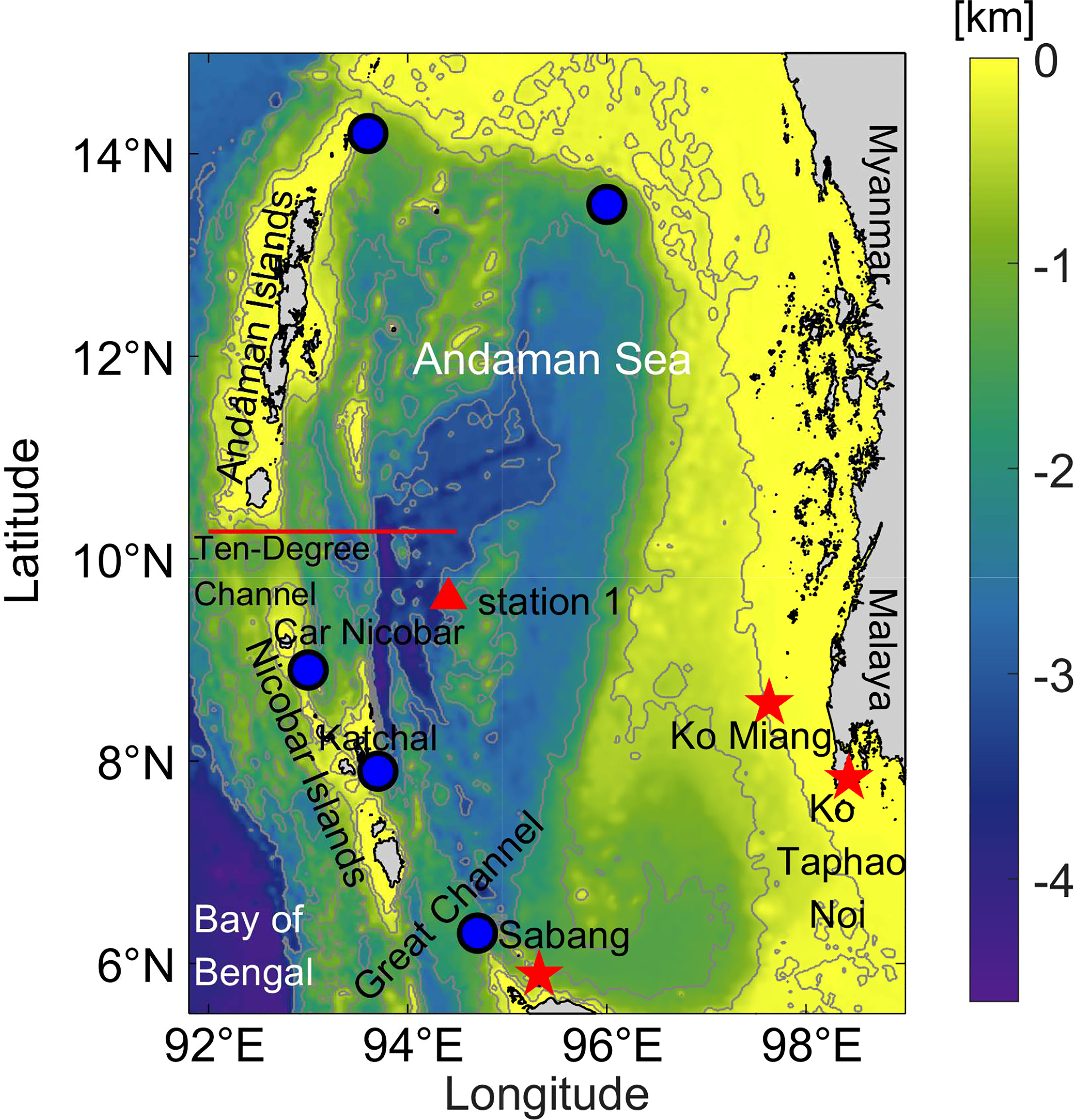
Figure 1 Bathymetry map of the model domain. Bathymetry contours are spaced at 100, 500, 1200, 2000, and 3000 m. The red stars represent the three observed stations in the Andaman Sea. The red line indicates one of the major paths of internal tides in the Andaman Sea. The red triangle illustrates the selected section to show the internal tidal form. The blue circles denote the potential generation regions of internal tides (Raju et al., 2019).

The outline of this study is as follows: The numerical model setup and results’ validations are described in Section 2. Tidal features in the Andaman Sea and theoretical frameworks are presented in Section 3. Section 4 is the results and discussion of the numerical model, including internal tidal form, generation sites, energy conversion and radiation, etc., in the generation and propagation processes. Conclusions and discussions are given in Section 5.

2. Numerical mode

2.1. Model setup

To examine the energy distribution and dynamical mechanism in the generation and propagation of internal tides in the Andaman Sea, we use the MITgcm (Massachusetts Institute of Technology General Circulation Model) model to conduct a high-resolution, three-dimensional, non-linear, hydrostatic approximation simulation. Orthogonal curvilinear coordinates are selected in the horizontal direction, and the classic z coordinate is selected in the vertical direction. The simulation domain is 5.5°–15°N to 91.8°–99°E. The bottom topography is derived from ETOPO1 dataset with the spatial resolution of (1′)×(1′) (Figure 1). Since the propagation of internal tides over the Andaman Sea is principally along the east-west direction, and the wavelengths are typically tens of kilometers, here the grid resolution is set to be (approximately) 500 m in the x direction and 1000 m in the y direction to achieve a balance between high resolution and accuracy. To capture the features of internal tides in the vertical column, we adopt more grids for the upper ocean than the lower ocean to achieve a balance between accuracy and efficiency. There are 150 layers with an entire depth of 4620 m, ranging from 1 m in each layer near the sea surface to 200 m near the bottom. The minimum depth of topography is set as 10 m to ensure the stability of the simulation, and the time step size is set as 10 s to satisfy the Courant–Friedrichs–Lewy (CFL) condition. An implicit free surface condition is implemented on the simulations, and the diffusion of temperature and salinity are set to be zero; a similar configuration can be found in many other numerical simulations on internal waves, for example, (Wang et al., 2016; Mohanty et al., 2018; Jithin et al., 2020; Peng et al., 2021). The horizontal and vertical viscosity parameters are chosen homogeneously over the entire simulated area with A_h = 10^-3 m²/s and A_z = 10^-6 m²/s, and to resolve the energetics of the phenomena whose spatial scale is smaller than the grid size, the nonlocal K-Profile Parameterization scheme (Large et al., 1994) is invoked based on the sensitivity experiments we have conducted (not shown).

Based on MODIS images, Sun et al. (2019) conducted some statistical analyses, which suggested that internal waves occurred at the highest frequency in spring, especially in March, while at the lowest frequency in June and July. Therefore, we simulate the internal tides in the Andaman Sea in March, ranging from 1 March to 31 March 2006, including two complete spring and neap tidal cycles. The initial temperature and salinity (Figure 2) fields are set horizontally homogenous, and the data are extracted from the World Ocean Atlas 2018 (WOA18) dataset. In the upper 1500 m, we choose the monthly average in March, and below 1500 m, we choose the seasonal average. Buoyancy frequency $N=\sqrt{-\frac{g}{\overline{\rho }}\frac{d\rho }{dz}}$, where density ρ can be calculated according to the state equation of seawater EOS80 (UNESCO, 1981), $\overline{\rho }$ is the vertical average of density, z points upward, and g is the gravitational acceleration.

FIGURE 2

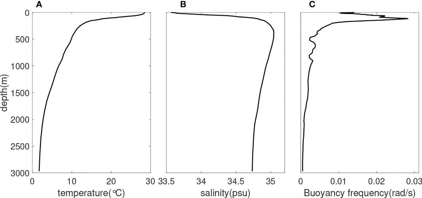
Figure 2 Vertical profiles of initial (A) temperature, (B) salinity, and (C) buoyancy frequency.

The barotropic tides are used at the four open boundaries, which are derived from the Oregon State University TOPEX/Poseidon Solution (TPXO8-atlas data) 1/30 degree (Egbert and Erofeeva, 2002). We set up 20 grids at the boundaries as the sponge layers, i.e., 10 km in the east-west direction and 20 km in the south-north direction. To compare the contribution of semidiurnal internal tides and diurnal internal tides in the Andaman Sea, we conducted three experiments. Specifically, theyare as follows: the experiments driven by the eight main tides (M2, S2, N2, K2, K1, O1, P1, and Q1), the experiments driven by the four main semidiurnal tides (M2, S2, N2, and K2), and the experiments driven by the four main diurnal tides (K1, O1, P1, and Q1). In all simulations, the salinity and temperature profile are set to be horizontally homogeneous, as in Zeng et al. (2019). To validate the model’s accuracy, we also carry out barotropic experiments. The vertical layers decrease to 40 and thermohaline iteration is closed to reduce the computational resources. When the barotropic tidal experiments are conducted, the temperature and salinity are set to be equal throughout the simulated domain, respectively (temperature 7°C, salinity 35 PSU). The simulation duration is extended to 120 days, and other settings are the same as the experiments driven by the eight main tides. Note that detailed configurations of the four numerical experiments are listed in Table 1.

TABLE 1

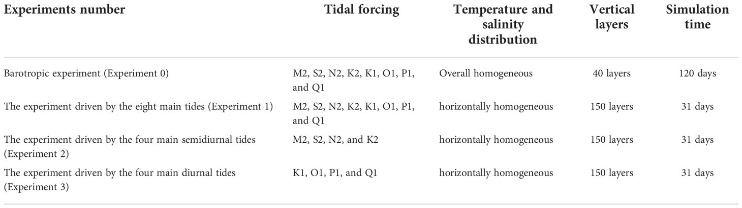
Table 1 The configurations of different numerical experiments.

2.2. Model validation

2.2.1. Barotropic tidal validation

We select the results of barotropic sea surface elevation and zonal barotropic velocity from day 16 to day 120 in Experiment 0 and carry out harmonic analysis using the T-Tide toolkit (Pawlowicz et al., 2022) to obtain the amplitude and phase of thetidal constituent and compare them with TPXO8-atlas data. As the M2 and S2 components are the most powerful among all tidal constituents, we show the comparison of the barotropic sea surface elevation and zonal barotropic velocity of M2 and S2 componentsbetween the model results and TPXO8 data in Figure 3.

FIGURE 3

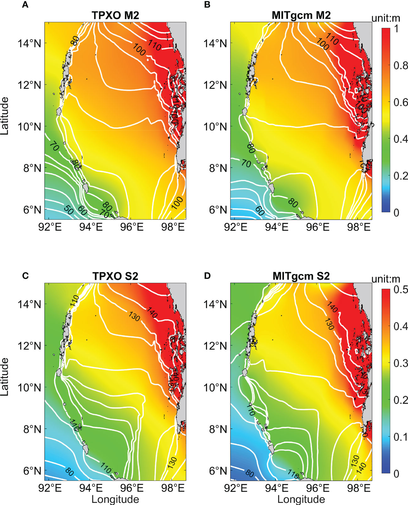
Figure 3 M2 and S2 cotidal charts for the barotropic tides based on the (A, C) TPXO and (B, D) simulation results. The colors indicate the amplitude, and the contours represent the phase. The color scale of M2 cotidal chart ranges from 0 to 1 m, and the color scale of S2 cotidal chart ranges from 0 to 0.5 m.

It is clear that, as shown in Figure 3, the model results are consistent with those of TPXO8 in terms of the co-tidal charts of sea surface elevation, especially in the Andaman and Nicobar Archipelago of the western Andaman Sea near the generation sites of the internal tides. The surface elevation distribution is slightly different in the northern Andaman Sea, where the amplitudes of M2 and S2 tidal constituents obtained from the model results are smaller than those derived from TPXO8, likely due to the difference in bathymetry and the resolution between ETOPO1 and TPXO8. The absolute root-mean-square error (RMSE) can comprehensively evaluate the biases of amplitude and phase for each tidal harmonic (Cummins and Oey, 1997), which is given by

$\begin{array}{ll}{E}_{ARMS}=\sqrt{\frac{1}{2}(A_0^2+A_m^2)-A_0{A}_m·\cos \text{ (}{g}_0-g_m)},& (1)\end{array}$

where A₀ and A_m represent the velocity amplitude derived from TPXO8 and MITgcm, respectively, g₀ and g_m represent the corresponding phase. In Figure 4, the E_ARMS for most parts of the Andaman Sea are less than 0.1m/s, and the E_ARMS is larger in the east near-coastal area partly due to the bathymetry is abrupt. Overall, the model is adequate to simulate the barotropic tides of the Andaman Sea.

FIGURE 4

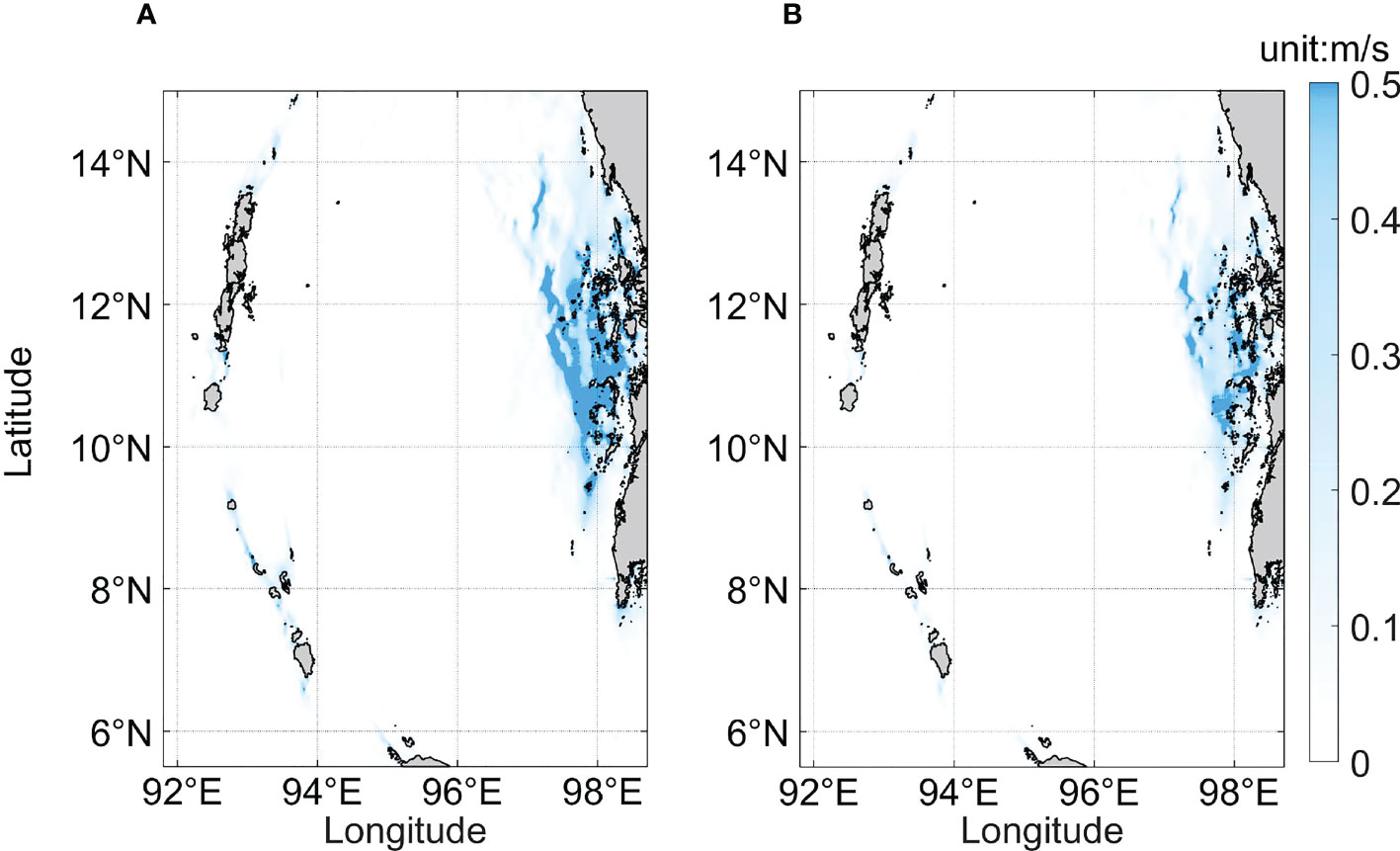
Figure 4 EARMS of zonal velocity of (A) M2 tidal constituent and (B) S2 tidal constituent.

2.2.2. Comparison with observations

Additionally, the model-simulated barotropic sea surface elevations are compared with the field observations at three tide stations (see red stars in Figure 1) near Sumatra and Malay derived from the University of Hawaii Sea Level CENTER (UHSLC). Generally, the amplitude and phase of model-simulated barotropic sea level around spring tide agree well with tide gauge data and TPXO8 (see Figure 5). Specifically, the amplitude of simulated elevation around spring tide at Ko Taphao Noi is slightly higher than that of observations, but the phase matches well. TPXO8-atlas data does not contain the elevation information at Sabang due to its low resolution, so we only compare model-simulated elevation and tide gauge data from UHSLC at this station. The simulated elevation around neap tide at Sabang (at a water depth of 5 m) shows a slight discrepancy with the observational data, probably because there are differences between the bathymetry data and the real topography. In summary, the model-simulated results match well with the observations, suggesting the model is qualified to reproduce the tidal characteristics of the Andaman Sea.

FIGURE 5

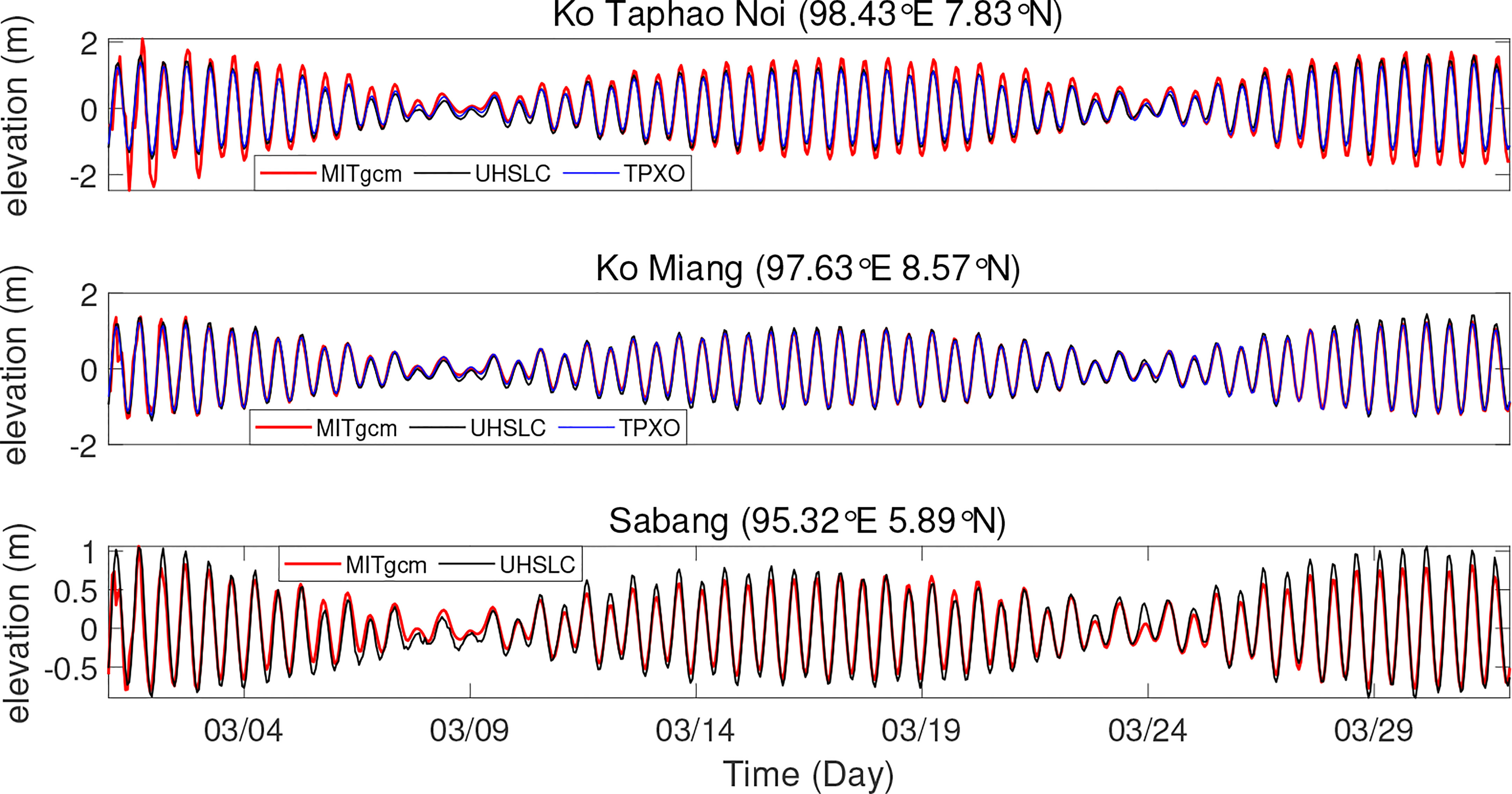
Figure 5 The comparisons of barotropic sea levels between model results and observations (locations are marked as red stars in Figure 1). The red line represents model-simulated elevation, the black line represents the tide gauge data from UHSLC, and the blue line represents the data of TPXO8 from 1 March to 31 March.

3. Theoretical framework

To characterize barotropic tides in the Andaman Sea, we select Station 1, located in one of the main propagation paths of internal tides (see the red triangle in Figure 1). We present local zonal barotropic velocity and barotropic sea surface elevation. Figure 6 indicates the dominance of semidiurnal tidal constituents at the local site. The maximum zonal barotropic velocities of the eight main tides in Experiment 1 and the four main semidiurnal barotropic tides in Experiment 2 during the spring tide period are about 0.04 m/s. Whereas the velocity for the case of the four main diurnal barotropic tides in Experiment 3 is about 0.003 m/s, which is one order of magnitude smaller. This phenomenon is similar during the neaptide period. For the zonal barotropic velocity, the time series of the eight main tides match well with that of the four main semidiurnal barotropic tides during spring tide. However, the zonal barotropic velocity of the eight main tides is sometimes lower than that of the four main semidiurnal barotropic tides during neap tide. The barotropic sea surface elevation shows similar circumstances at this station. It can be seen from the characteristics of barotropic tides that the semidiurnal tidal constituents are significantly stronger than the diurnal tidal constituents in the whole tidal cycle, and the gap between them is slightly smaller during neap tide. However, the baroclinic energy of internal tides excited by the two tidal constituents in the following calculation shows that the semidiurnal tidal energy is superior to diurnal tidal energy, and they can differ by order of magnitude even during neap tide.

FIGURE 6

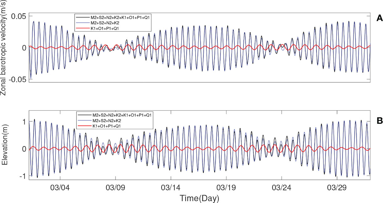
Figure 6 The time series of (A) model-simulated zonal barotropic velocity for Experiment 1 – 3 and (B) barotropic sea surface elevation derived from TPXO8 from 1 March to 31 March at Station 1 (see the red triangle in Figure 1), among which the black curve represents the eight main tides, the blue curve represents the four main semidiurnal tides, and the red curve represents the four main diurnal tides.

In this paper, the tidally averaged baroclinic energy balance equation (Cummins and Oey, 1997; Kang and Fringer, 2012) is applied to analyze the generation and propagation processes of internal tides in the Andaman Sea, which is written as

$\begin{array}{ll}\frac{\partial }{\partial t}\left(\langle KE\rangle +\langle APE\rangle \right)+\nabla ·\langle \mathit{F}\rangle =\langle C\rangle -\langle D\rangle -\langle M\rangle ,& (2)\end{array}$

where ⟨⟩ indicates depth integration. $KE=\frac{1}{2}{\rho }_0(u^{\text{'}2}+v^{\text{'}2}+w^2)$denotes the baroclinic kinetic energy, where u′ and v′ are baroclinic horizontal zonal velocity and meridional velocity, respectively, which can be obtained by subtracting the barotropic components (U) from the total velocity (u). That is to say, u′=u–U and $\mathbf{U}=\frac{1}{H+\eta }{\displaystyle {\int }_{-H}^{\eta }\mathit{\text{u}}dz}$, where η and H are the free surface elevation and bottom depth, respectively. w is vertical velocity, and ρ₀ is reference density. APE = g² ρ^′2/(2ρ₀N²) denotes available potential energy, in which ρ′ =ρ(x, y, z, t)–ρ_b(z) is the perturbation density and ρ_b(z) is the background density.

The third term of equation (2) represents the divergence of the baroclinic energy flux, which is calculated as follows

$\begin{array}{ll}\langle \mathit{\text{F}}\rangle =\langle {\mathit{\text{u}}}^{\prime }{p}^{\prime }\rangle +\langle \mathit{\text{u}}KE\rangle +\langle \mathit{\text{u}}K{E}_0\rangle +\langle \mathit{\text{u}}APE\rangle -\langle K_h\nabla KE\rangle -\langle A_h\nabla APE\rangle .& (3)\end{array}$

p′ is the perturbation pressure, which is given by

$\begin{array}{ll}{p}^{\prime }={\displaystyle {\int }_z^{\eta }{\rho }^{\prime }(\widehat{z},t)gd\widehat{z}-\frac{1}{H+\eta }{\displaystyle {\int }_{-H}^{\eta }{\displaystyle {\int }_z^{\eta }{\rho }^{\prime }(\widehat{z},t)gd\widehat{z}dz,}}}& (4)\end{array}$

and KE₀ = ρ₀(Uu′+Vv′). K_h and A_h are the horizontal eddy diffusivity and viscosity parameters, respectively (Wang et al., 2018).

C= ρ′gW is the barotropic-to-baroclinic energy conversion rate, the positive values of which are the sources of internal tidal energy. W=−∇·[(H+z)U] is vertical barotropic velocity.

The following two parameters are calculated to evaluate whether the regions with high barotropic-to-baroclinic energy conversion rates are the internal tides generation sites

Slope criticality:

$$\alpha =\frac{\frac{dh}{dx}}{\sqrt{\frac{{\omega }^2-f^2}{N^2-{\omega }^2}}},$$

where h(x) is the bathymetry, ω is the tidal frequency, and f =2ϖsinφ is the Coriolis parameter, with ϖ the Earth’s rotational angular velocity and φ the corresponding latitude (Gilbert and Garrett, 1989; 206 Shaw et al., 2009).α >1, α =1, and α<1 represent supercritical, critical, and subcritical ridges, respectively. When α >1 internal tides are possibly generated (Hurley and Keady, 1997; Zhang et al., 2007).

Internal tide generating body force or Baines force:

$$F_{body}=\frac{\mathit{\text{Q}}·\nabla (1/h)}{\omega }{\displaystyle {\int }_{-H}^{\eta }z{N}^2(z)dz,}$$

in which Q =(Uh, Vh) is barotropic mass flux vector, and ∇ is the horizontal gradient operator. Internal tides are often generated where F_body is large (F_body >0.25m²/s²) (Lozovatsky et al., 2012; Raju et al., 2019).

4. Results and discussion

4.1. Internal tides form

The sections of modelled zonal baroclinic velocity and isotherms of semidiurnal internal tides and diurnal internal tides along 10.27°N are shown in Figure 7. There are evident internal tides beam of semidiurnal internal tides from 92.5°E to 94°E, while the diurnal internal tidal signals are relatively weak. In terms of isothermal displacements of 18°C, the amplitude of semidiurnal internal tides is about 40 m. In contrast, its counterpart, diurnal internal tides, is only about 4 m (see Figure 8). The two ridges located at 92.3°E and 92.7°E are capable of generating semidiurnal internal tides, which propagate east-westward (see Figure 8A). In Figure 8A, the distribution and propagation of semidiurnal internal tides can be clearly observed, characterized by east-west radiations in the entire model domain. The Andaman and Nicobar Archipelago are the main generation sites of semidiurnal internal tides. The fluctuation signals of the diurnal internal tides are not obvious (see Figure 8B), and there are no evident diurnal tidal generation sites.

FIGURE 7

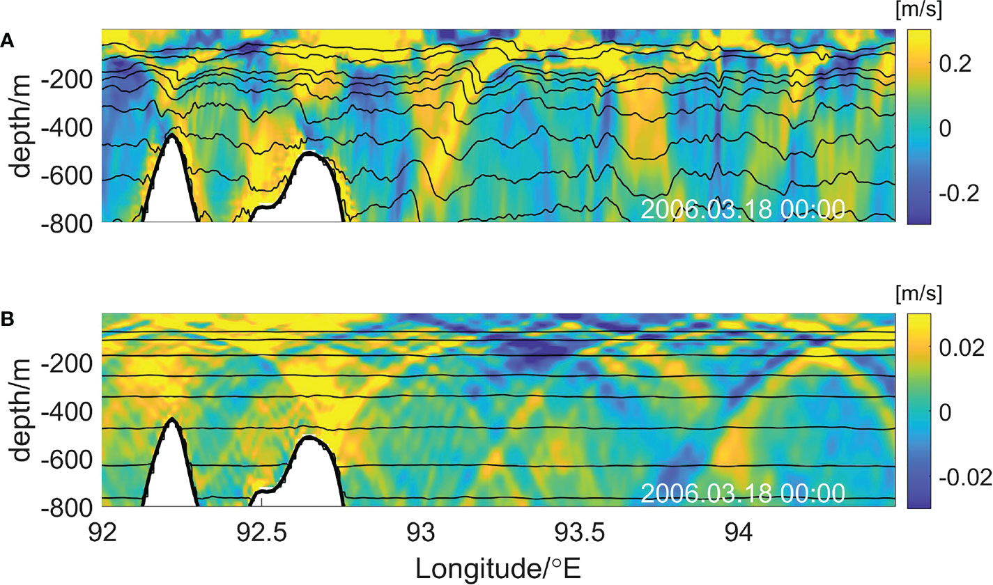
Figure 7 Selected section along 10.27°N (see the red line in Figure 1) of (A) semidiurnal internal tides and (B) diurnal internal tides showing modelled zonal baroclinic velocity (u ′, colour coded in m/s on the right-hand side) dated 18 March 2006 at 00:00. The solid black lines are isotherms. Note that the color scales in the two panels are different.

FIGURE 8

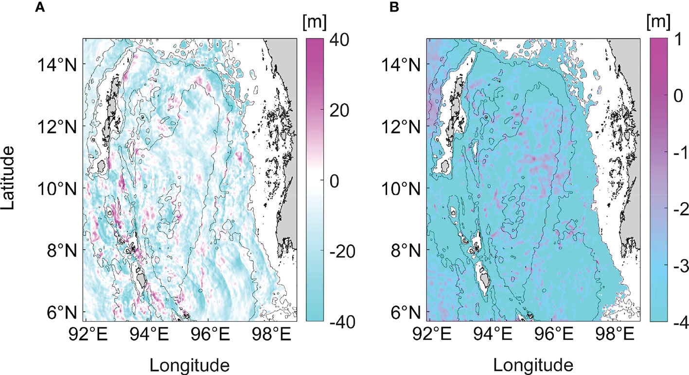
Figure 8 A snapshot of the model-predicted isothermal displacements of 18°C for (A) semidiurnal internal tides and (B) diurnal internal tides at 00:00 on 18 March 2006. Bathymetry contours are spaced at 100, 500, and 2000 m. The blank space represents the shelf. Note that the color scales in the two panels are different.

4.2. Generation of internal tides

4.2.1. Energy distribution

To evaluate the different characteristics of internal tides during spring and neap tide, we select 15-16 March as the spring tide period and 23-24 March as the neap tide period, respectively, for calculation (see Figure 6). The generation of internal tides is accompanied by energy conversion from barotropic to baroclinic tides. Figure 9 shows spatial distributions of the time-averaged depth-integrated barotropic-to-baroclinic conversion rate during the spring and neap tide periods. The positive barotropic-to-baroclinic energy conversion rate represents the generation of internal tidal energy, and the negative means the reverse conversion from baroclinic to barotropic tides (e.g., Zilberman et al., 2009; Kerry et al., 2013; 233 Nagai and Hibiya, 2015). During the spring tide, the total barotropic-to-baroclinic energy conversion rate of the Andaman Sea is 29.15 GW in Experiment 1, 29.24 GW in Experiment 2, and 0.05 GW in Experiment 3, respectively. During the neap tide, the total barotropic-to-baroclinic energy conversion rate of the Andaman Sea is 3.08 GW in Experiment 1, 2.56 GW in Experiment 2, and 0.31 GW in Experiment 3, respectively. It can be seen that semidiurnal tidal energy is dominant since there is little difference between the energy conversion rate in Experiment 1 and Experiment 2. Four regions denoted as A, B, C, and D with high barotropic-to-baroclinic energy conversion rates are marked as black boxes in Figure 9. They are close to those found by Mohanty et al. (2018) and Raju et al. (2019), indicating the four main generation sites of internal tides in the Bay of Bengal. Note that in some regions, see Figures 9D, E, the conversion rate is negative, which can be generally attributed to the phase (greater than 90 degree) difference between the baroclinic pressure and vertical barotropic velocity. When the remotely-generated internal tides are dominant at the local site, the local pressure can be significantly influenced, thereby resulting in the negative conversion rate. It can be seen in Figure 9D, these negative conversions occured in domains B and C, where the remotely-generated internal tides are relatively strong. As the disturbance pressure of the remote internal tides and the local vertical barotropic velocity are out of phase, the conversion rate is negative, see Zilberman et al. (2011); Gong et al. (2019) for similar scenarios.

FIGURE 9

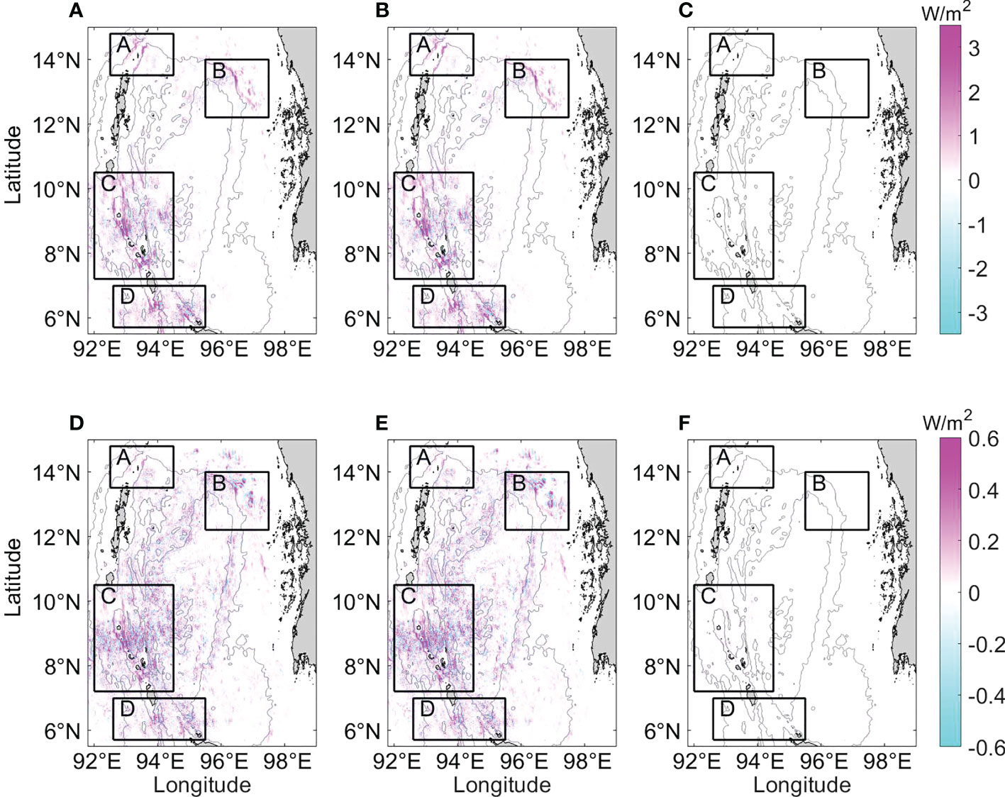
Figure 9 Spatial distributions of the time-averaged depth-integrated barotropic-to-baroclinic conversion rate in the (A, D) Experiment 1, (B, E) Experiment 2, and (C, F) Experiment 3. The period of (A ∼ C) is spring tide, and the range of color scale is −3.5 ∼ 3.5 W/m²; the period of (D ∼ F) is neap tide, and the range of color scale is −0.6 ∼ 0.6 W/m². The four rectangles present the main generation subdomains of internal tides. Bathymetry contours are spaced at 500 and 2000 m.

4.2.2. Generation regions

4.2.2.1. Slope criticality

Slope criticality is related to the period of tidal constituents. In the Andaman Sea, the M2 tidal constituent is the strongest among whole semidiurnal tidal constituents, and the K1 tidal constituent is the strongest among whole diurnal tidal constituents. The distribution of slope criticality greater than 1 of these two tidal constituents is shown in Figure 10. The high values of slope criticality of the M2 tidal constituent (in Figure 10) are mainly distributed in the Andaman and Nicobar Archipelago, northwest Sumatra, and the northeast Andaman Sea, close to the four regions with high barotropic-to-baroclinic energy conversion rate (Figure 9). For the K1 tidal constituent, the frequency of which is about half that of the M2 tidal constituent, and the angle between the internal tides beam and the horizontal direction excited by which is smaller than that excited by the M2 tidal constituent, so the distribution of high slope criticality is more extensive (Figure 10A).

FIGURE 10

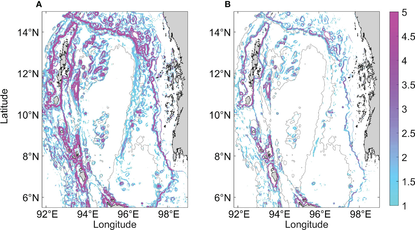
Figure 10 Slope criticality of (A) K1 tidal constituent and (B) M2 tidal constituent. Bathymetry contours are spaced at 500 and 2000 m.

4.2.2.2. Internal tide generating body force

The high body force regarding K1 and M2 tidal constituents is located in the vicinity of the Andaman and Nicobar Archipelago and northeastern Andaman Sea (Figure 11), which shows similar spatial patterns to slope criticality. It is noted that the body force of the M2 tidal constituent in the northeastern Andaman Sea is also high, as shown in Figure 11B, indicating that M2 internal tides can be generated here. However, the topography in these areas is shallow and abrupt, so the generated internal tides dissipate within a short distance (see Figure 8A). The body force of the K1 tidal constituent is smaller than that of the M2 tidal constituent, demonstrating that the formation of diurnal internal tides is limited. The areas with body force greater than 0.25m²/s² regarding the M2 tidal constituent account for 33% of the model domain, and those regarding the K1 tidal constituent account for 17%. As internal tides are mainly generated where F_body>0.25m²/s², the M2 internal tides are more likely to be generated in the Andaman Sea.

FIGURE 11

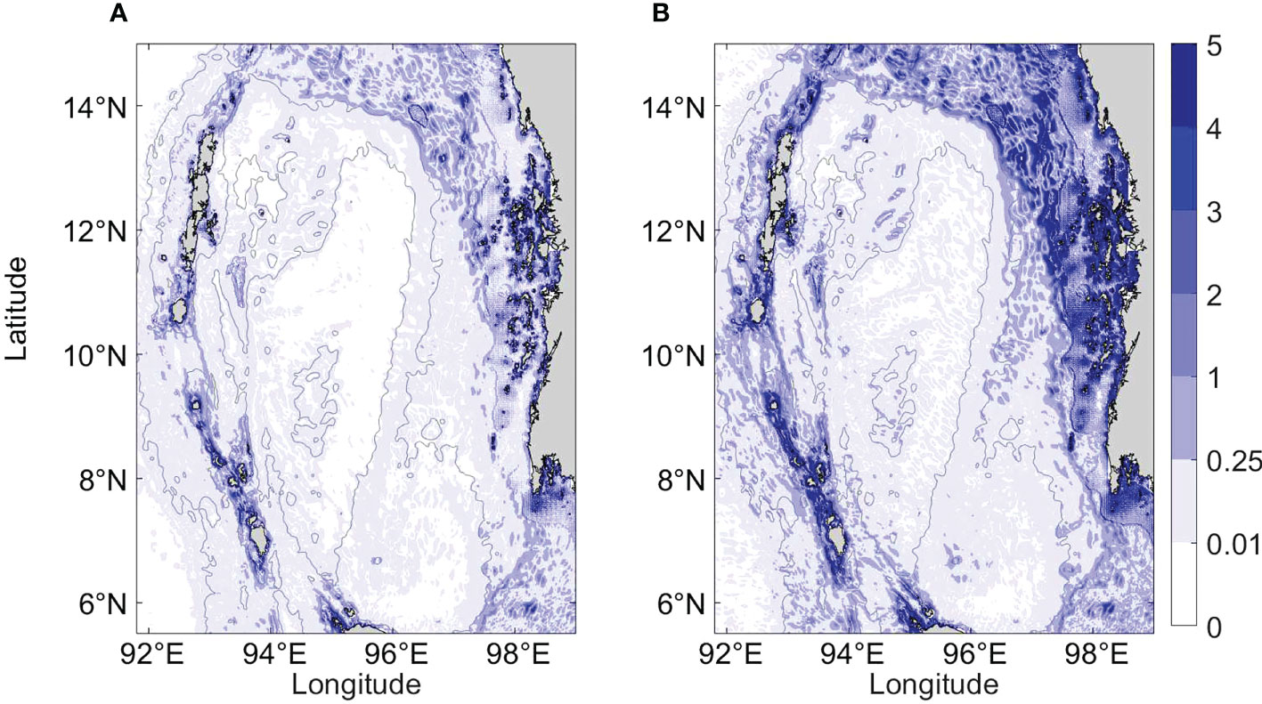
Figure 11 Maximum absolute value of depth-integrated internal tide generating body force of (A) K1 tidal constituent and (B) M2 tidal constituent in March. Bathymetry contours are spaced at 500 and 2000 m.

4.3. Propagation of internal tides

4.3.1.. Energy distribution

To further determine the generation regions of internal tides, we calculate the internal tidal energy budget following equation (3). we find that the magnitude of the first pressure term is much larger than the other five terms. Note that the following results are the comprehensive results of these six terms. The distribution of baroclinic energy flux in Experiment 2 (Figures 12B, E) is similar to that in Experiment 1 (Figures 12A, D), while that in Experiment 3 is indistinguishable (Figures 12C, F). The energy propagating direction of internal tides is mainly east-west, and the maximum value appears near the generation regions in Experiment 1.

FIGURE 12

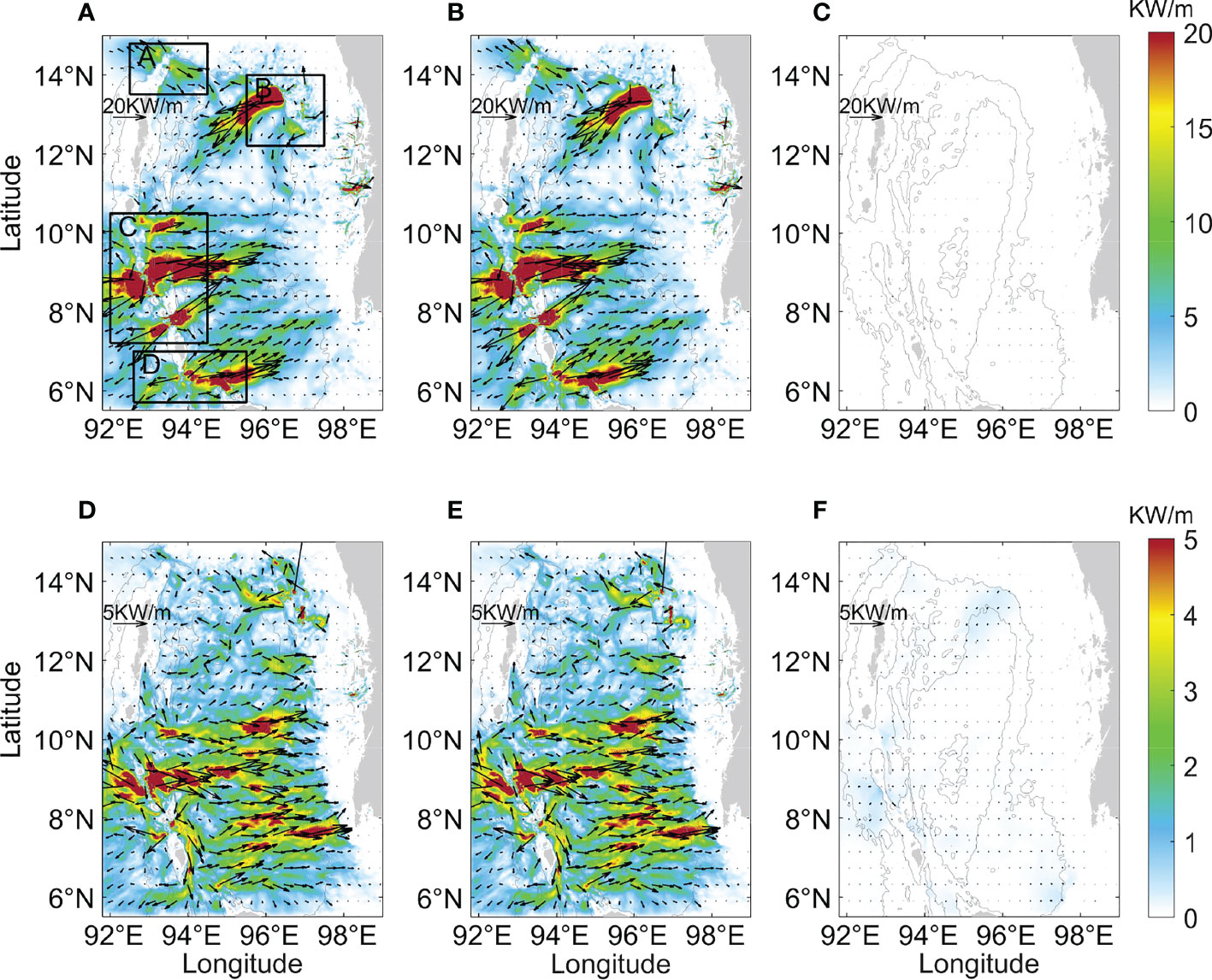
Figure 12 Spatial distribution of the time-averaged depth-integrated baroclinic energy flux in the (A, D) Experiment 1, (B, E) Experiment 2, and (C, F) Experiment 3. The period of (A–C) is spring tide, and the range of color scale is 0~20KW/m; the period of (D–F) is neap tide, and the range of color scale is 0~5KW/m. The color shade indicates the magnitude of the baroclinic energy flux, and the arrows indicate the direction of the baroclinic energy flux. The four rectangles in the panel (A) present the main generation subdomains of internal tides. Bathymetry contours are spaced at 500 and 2000 m.

In Figures 12A, B, the radiation sources of baroclinic energy are obvious during spring tides, mainly located in the Andaman and Nicobar Archipelago and the northeastern Andaman Sea, namely the four regions in Figure 9. The baroclinic energy flux in Experiment 1 in subdomain C is significantly large (>20KW/m) and propagates at a relatively long distance (200 km). It can be seen that the energy flux can propagate both westward and eastward, butthe energy decreases rapidly when crossing 92°E and 95.5°E, respectively. There are three apparent energy sources in the vicinity of the ten-degree channel, Car Nicobar and Katchal. Among them, the south of Car Nicobar is the strongest site (see Figure 13A). Baroclinic energy flux around the northern Andaman Islands (subdomain A) is the smallest compared with the other three subdomains and mainly propagates northwestward and southeastward. The northwestward energy radiates into the northern Bay of Bengal and then interferes with local internal tides. The southeastward energy dissipates after propagating a distance of 20 km. The baroclinic energy in subdomain B mainly propagates southwestward, then interference with that from subdomain A near 94.8°E. In northwestern Sumatra (subdomain D), the propagation direction of baroclinic energy flux is also mainly east-westward, and the eastward energy issignificantly higher than the westward energy. The eastward baroclinic energy flux decreases sharply when crossing 95.7°E and gradually turns northeastward around 96°E. In the east of the Andaman Sea and west of Myanmar, the baroclinic energy can also be observed in the vicinity of 11~13°N, 98.2°E. Although baroclinic tides can be motivated over the complicated local topography,they only radiate away within a short distance and dissipate quickly.

FIGURE 13

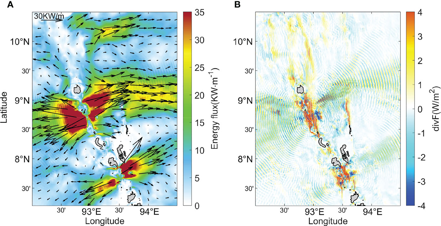
Figure 13 The distribution of (A) baroclinic energy flux and (B) the divergence during the spring tide period in the subdomain C in the Experiment 1.

The baroclinic energy flux during neap tide (Figures 12D, E) is smaller than that during spring tide (Figures 12A, B). The radiation sources of energy are scattered during the neap tides, and regions with high values of energy fluxes are mainly located in the southern Andaman Sea. The baroclinic energy flux in the southern Car Nicobar is still large, and the east-west propagation characteristics can also be seen. Still, the characteristics in the other three subdomains, especially in subdomain A, are not obvious.

The propagation of internal tides is accompanied by energy radiation and dissipation. By averaging over several tidal cycles, baroclinic energy is approximately equal to the sum of baroclinic energy flux divergence and baroclinic dissipation rate, namely $\langle \overline{C}\rangle =\langle \overline{\nabla ·F}\rangle +\langle \overline{D+M}\rangle$, where $\langle \overline{D+M}\rangle$ is the dissipation term and $\overline{( )}$ represents time average. In Figure 14, there is little difference between the baroclinic energy flux divergence in Experiment 1 and Experiment 2 compared with Experiment 3 during the spring and neap tide period. The baroclinic energy flux divergence of semidiurnal internal tides is three orders of magnitude larger than that of diurnal internal tides during the spring tides, while it is one order of magnitude larger than diurnal internal tides during the neap tides, similar to the barotropic-to-baroclinic energy conversion rate. The large values of divergence are mainly located at the generation sites of internal tides, and the distribution of which is similar to that of barotropic-to-baroclinic conversion rate, slope criticality, and body force. There is a lot of negative divergence during neap tide in the eastern Andaman Sea, corresponding to the local energy dissipation of internal tides in high modes. In Figures 14A, B, the largest baroclinic conversion rates occur in subdomain C during spring tide, and the percentage of energy flux divergence to the conversion rate (44%) is the smallest among the four subdomains, indicating that the relative dissipation is largest. The dissipation $\langle \overline{D+M}\rangle$ in subdomain C is about 56% during spring tide, demonstrating that half baroclinic energy of the rest will dissipate. The barotropic-to-baroclinic conversion rate and energy flux divergence in Experiment 2 are larger than in Experiment 1 in some regions, likely due to the out-phase of semidiurnal internal tides and diurnal internal tides. Moreover, the energy budget in the Andaman Sea is calculated during the entire tidal period (Figure 15), suggesting that the 14-day time-averaged energy flux divergence is always lower than the barotropic-to-baroclinic conversion rate in all three experiments. Nonetheless, the energy terms of diurnal internal tides are two orders of magnitude lower than that of semidiurnal internal tides.

FIGURE 14

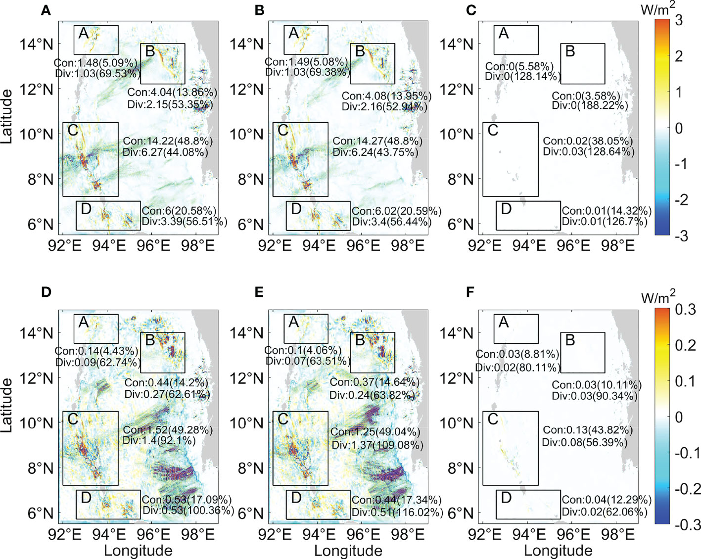
Figure 14 Spatial distribution of the time-averaged depth-integrated baroclinic energy flux divergence in the (A, D) Experiment 1, (B, E) Experiment 2, and (C, F) Experiment 3. The period of (A–C) is spring tide, and the range of color scale is –3~3W/m²; the period of (D–F) is neap tide, and the range of color scale is –0.3~0.3W/m². The four rectangles present the main generation subdomains of internal tides. Con represents the barotropic-to-baroclinic energy conversion rate of the corresponding subdomain (unit: GW), and the percentage of that to the total barotropic-to-baroclinic energy conversion rate in the Andaman Sea is shown in brackets. Div represents the baroclinic energy flux divergence of the corresponding subdomain (unit: GW), and the percentage of that to the barotropic-to-baroclinic energy conversion rate of the corresponding subdomain is shown in brackets.

FIGURE 15

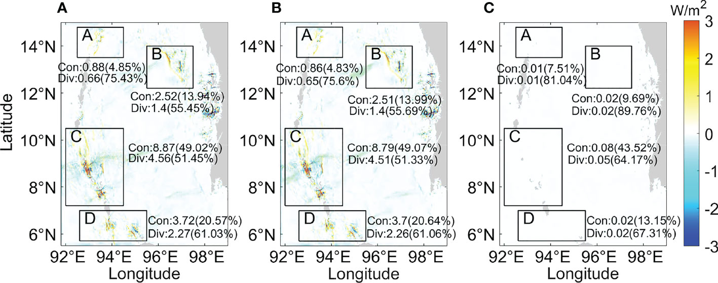
Figure 15 Same as Figures 14A–C, but during the entire tidal period (14 days).

4.3.2. Energy budget

In Figure 16, there are two peaks of barotropic-to-baroclinic energy conversion rate of both semidiurnal internal tides and diurnal internal tides during their tidal period (Figures 16C2, C3, D2, D3). For semidiurnal internal tides, the first (second) peak within 12 hours is bigger during the spring (neap) tide. For diurnal internal tides, there is no apparent difference between the two peaks within 24 hours. In fact, the generation of internal tides corresponds to the time when the second extreme appears. The two peaks of the barotropic-to-baroclinic energy conversion rate of the whole Andaman Sea are more evident than that of subdomain C (Figures 16A1, B1). In Figures 17C3 and D3, there are also two peaks of baroclinic energy flux divergence of both semidiurnal internal tides and diurnal internal tides within their tidal period during the neap tide. However, in Figure 17C2, there are multiple peaks of semidiurnal internal tides within 12 hours during spring tide. The baroclinic energy among subdomain C accounts for almost half of that among the whole Andaman Sea (Figures 16A1, 16B1, 17A1 and 17B1). Both the barotropic-to-baroclinic energy conversion rate and baroclinic energy divergence show that the energy variations in Experiment 1 are similar to those in Experiment 2.

FIGURE 16

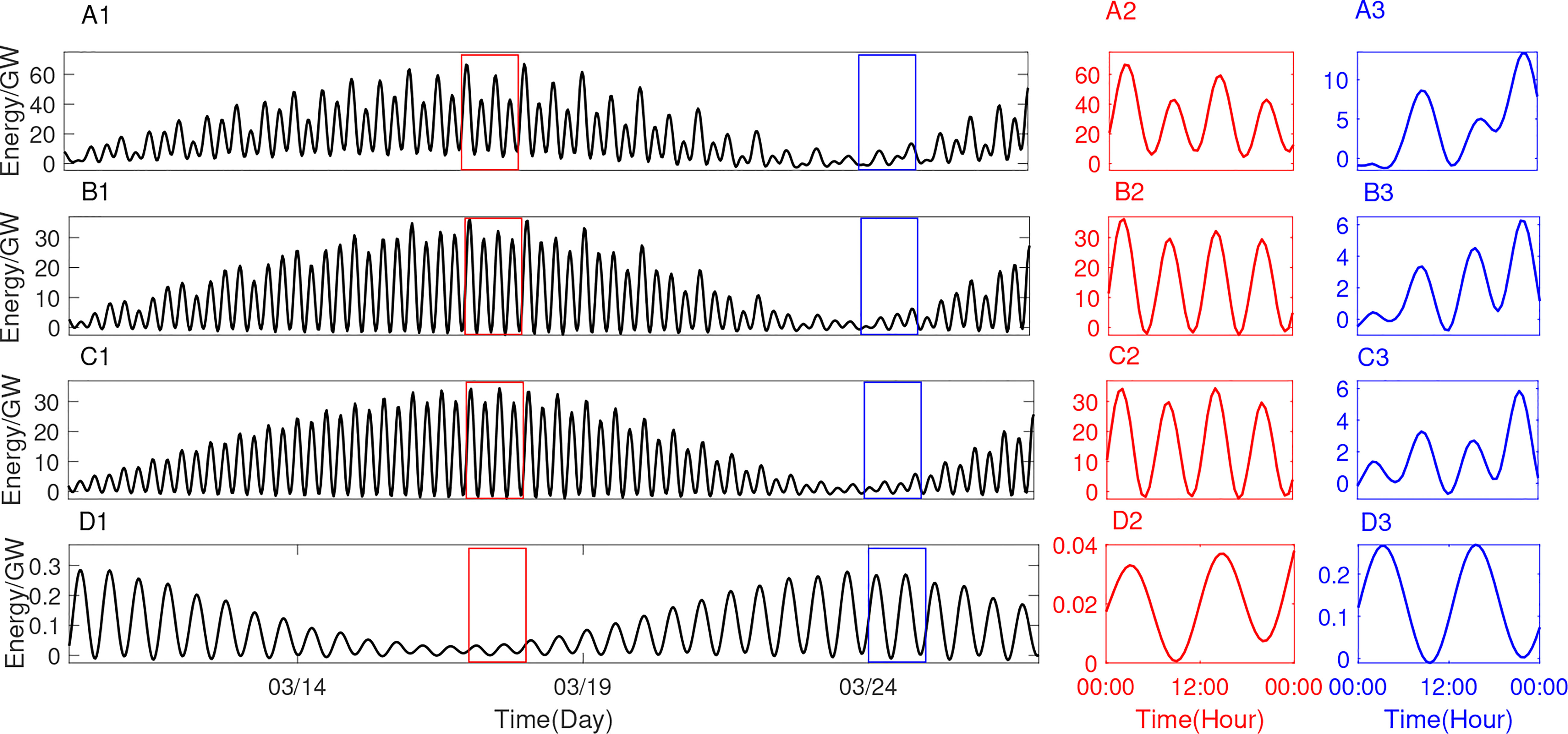
Figure 16 Time series of the barotropic-to-baroclinic energy conversion rate in the Andaman Sea, in which (A1 ∼ A3) is in the whole Andaman Sea in Experiment 1, (B1 ∼ B3) is in subdomain C in Experiment 1, (C1 ∼ C3) is in subdomain C in Experiment 2, and (D1 ∼ D3) is in subdomain C in Experiment 3. A2 (A3), B2 (B3), C2 (C3), and D2 (D3) are on March 17 (24), corresponding to the red (blue) rectangle in A1, B1, C1, and D1.

FIGURE 17

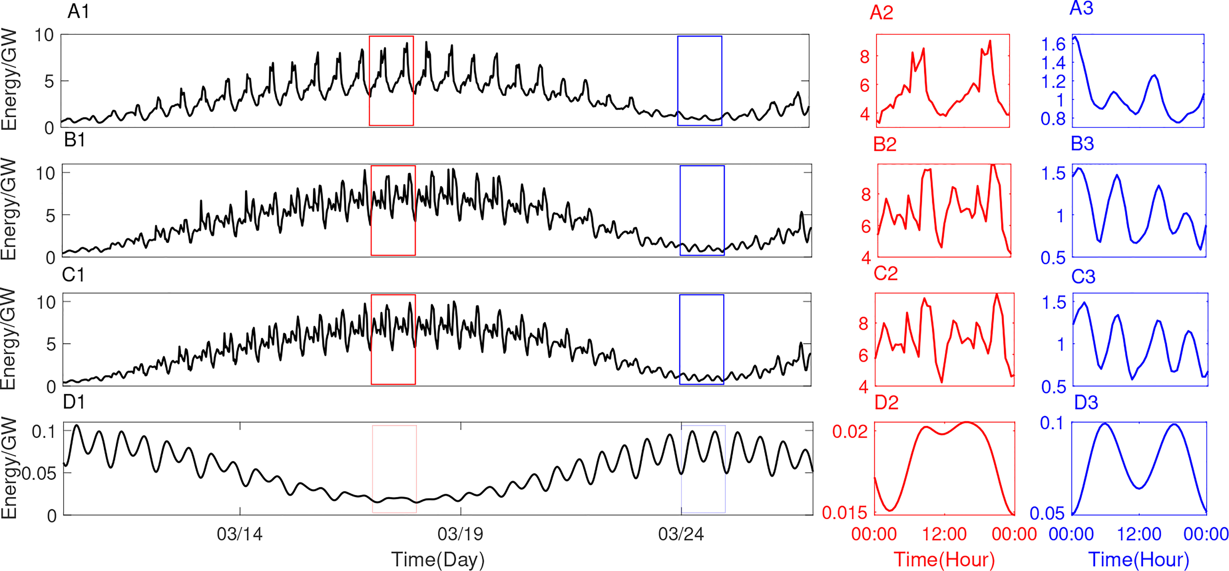
Figure 17 Same as Figure 16, but for baroclinic energy flux divergence.

5. Conclusions

In this study, a high-resolution three-dimensional MITgcm is configured to investigate the generation and propagation processes of internal tides in the Andaman Sea. The differences in spatial distributions and energy budgets between the semidiurnal and diurnal internal tides in the Andaman Sea are discussed. The semidiurnal internal tides are dominant in the Andaman Sea, and their intensity is not significantly different from that of the internal tides excited by eight main tides. Diurnal barotropic tides can independently reproduce internal tides, but the intensity of which is much weaker than that driven by semidiurnal components. The strength of diurnal barotropic tides (e.g., the maximum zonal barotropic velocity is 0.003 m/s at station 1 in Figure 1 during the spring tides period) is generally one order of magnitude smaller than that of the semidiurnal barotropic tides (e.g., the maximum zonal barotropic velocity is 0.04 m/s at station 1 in Figure 1 during the spring tides period). However, the energy of diurnal internal tides (e.g., the total barotropic-to-baroclinic energy conversion rate in the Andaman Sea is 0.05 GW) is about three orders of magnitude lower than that of semidiurnal internal tides (e.g., the total barotropic-to-baroclinic energy conversion rate in the Andaman Sea is 29.24 GW) during the spring tides. The energy of diurnal internal tides (e.g., the total barotropic-to-baroclinic energy conversion rate in the Andaman Sea is 0.31 GW) is about one order of magnitude lower than that of semidiurnal internal tides (e.g., the total barotropic-to-baroclinic energy conversion rate in the Andaman Sea is 2.56 GW) during the neap tides. Calculations for the entire tide period in the Andaman Sea show that the diurnal tidal energy is two orders of magnitude lower than the semidiurnal tidal energy. There are evident semidiurnal internal tides beam, while the diurnal internal tidal signals are relatively weaker. The amplitude of diurnal internal tides reflected by the isothermal fluctuation is also one magnitude lower than that of semidiurnal internal tides. In addition, there are two peaks of barotropic-to-baroclinic energy conversion rate of both semidiurnal internal tides and diurnal internal tides during their tidal period, and the generation of internal tides corresponds to the second peak. For semidiurnal internal tides, the first peak within 12 hours is larger around spring tide, and the second peak is larger around the neap tide.

Four potential generation regions of internal tides are found, mainly distributed in the Andaman and Nicobar Archipelago and the northeastern Andaman Sea. These regions satisfy the generation conditions by calculating slope criticality and internal tide generating body force. The distribution of baroclinic energy fluxes also shows that the internal tides are indeed generated in these subdomains and radiate outward. Among the four subdomains, the baroclinic energy in subdomain C accounts for about half of the whole Andaman Sea. Simultaneously, in the spring tides, most of the baroclinic energy is in the subdomain C, and more than half of the energy dissipates locally in this subdomain, contrasting to the subdomain A. Nevertheless, the baroclinic energy flux in subdomain C is significantly large (>20KW/m) and propagates over a relatively long distance (200 km). Inside subdomain C, we also find three obvious energy sources in the vicinity of the ten-degree channel, Car Nicobar and Katchal. In the neap tides, the baroclinic energy in region C is still large, and the generated internal tides propagate along the east-west direction; however, the energy contribution of the other three regions is much lower, especially region A. The internal tidal energy is mainly distributed in the southern Andaman Sea during this period. There are no evident diurnal internal tidal generation sites found, and the strength of the diurnal internal tides is also weak, which indicates that the inclusion of diurnal barotropic tides negligibly modulates the internal tides in the Andaman Sea.

In conclusion, this numerical study highlights the dominant semidiurnal internal tides in the Andaman Sea and the generation sites of internal tides. Moreover, understanding the generation mechanism of internal tides in the spring and neap tides and quantitatively identifying the tidal energy budget among the four regions in this study indeed give a complete story of internal tides during the generation, propagation, and dissipation processes in the Andaman Sea. Nonetheless, this work still leaves some questions which need to be further explored: the generation mechanism of the internal tides in the four subdomains identified; the radiating energy pathways after leaving the generation sites; the dynamical manner of the internal tides, especially its relationship with the large-amplitude nonlinear internal waves.

Data availability statement

Publicly available datasets were analyzed in this study. This data can be found here: https://www.tpxo.net/ https://ngdc.noaa.gov/mgg/global/global.html.

Author contributions

WW conducted the numerical simulations, performed the data analyses and wrote the manuscript. YG contributed significantly to the data analyses and manuscript preparation. ZW and CY conceived and designed the study, performed the data analyses and wrote the manuscript. All authors contributed to the article and approved the submitted version.

Funding

This work was supported by the National Natural Science Foundation of China (42006016, 12132018), the Fundamental Research Funds for the Central Universities (202265005), the Natural Science Foundation of Shandong Province (ZR2020QD063), the key program of the National Natural Science Foundation of China (91958206) and the National Natural Science Foundation of China (42206012).

Acknowledgments

The authors would like to thank the reviewers for their valuable suggestions on the manuscript.

Conflict of interest

The authors declare that the research was conducted in the absence of any commercial or financial relationships that could be construed as a potential conflict of interest.

Publisher’s note

All claims expressed in this article are solely those of the authors and do not necessarily represent those of their affiliated organizations, or those of the publisher, the editors and the reviewers. Any product that may be evaluated in this article, or claim that may be made by its manufacturer, is not guaranteed or endorsed by the publisher.

References

Alford M. H. (2003). Redistribution of energy available for ocean mixing by long-range propagation of internal waves. Nature 423, 159–162. doi: 10.1038/nature01628

PubMed Abstract | CrossRef Full Text | Google Scholar

Alpers W., Wang-Chen H., Hock L. (1997). "Observation of internal waves in the Andaman Sea by ERS SAR," IGARSS'97. 1997 IEEE International Geoscience and Remote Sensing Symposium Proceedings. Remote Sensing - A Scientific Vision for Sustainable Development,4, 1518–1520. doi: 10.1109/IGARSS.1997.608926

CrossRef Full Text | Google Scholar

Cummins P. F., Oey L.-Y. (1997). Simulation of barotropic and baroclinic tides off northern British Columbia. J. Phys. Oceanogr. 27, 762–781. doi: 10.1175/1520-0485(1997)027<0762:SOBABT>2.0.CO;2

CrossRef Full Text | Google Scholar

Egbert G. D., Erofeeva S. Y. (2002). Efficient inverse modeling of barotropic ocean tides. J. Atmos. Oceanic Technol. 19, 183–204. doi: 10.1175/1520-0426(2002)019<0183:EIMOBO>2.0.CO;2

CrossRef Full Text | Google Scholar

Egbert G. D., Ray R. D. (2000). Significant dissipation of tidal energy in the deep ocean inferred from satellite altimeter data. Nature 405, 775–778. doi: 10.1038/35015531

PubMed Abstract | CrossRef Full Text | Google Scholar

Fang X., Du T. (2005). Fundamentals of oceanic internal waves and internal waves in the China seas (Qingdao: China Ocean University Press).

Google Scholar

Gilbert D., Garrett C. (1989). Implications for ocean mixing of internal wave scattering off irregular topography. J. Phys. Oceanogr. 19, 1716–1729. doi: 10.1175/1520-0485(1989)019<1716:IFOMOI>2.0.CO;2

CrossRef Full Text | Google Scholar

Gong Y., Rayson M. D., Jones N. L., Ivey G. N. (2019). The effects of remote internal tides on continental slope internal tide generation. J. Phys. Oceanogr. 49, 1651–1668. doi: 10.1175/JPO-D-18-0180.1

CrossRef Full Text | Google Scholar

Hurley D. G., Keady G. (1997). The generation of internal waves by vibrating elliptic cylinders. part 2. approximate viscous solution. J. Fluid Mechanics 351, 119–138. doi: 10.1017/S0022112097007039

CrossRef Full Text | Google Scholar

Hyder P., Jeans D., Cauquil E., Nerzic R. (2005). Observations and predictability of internal solitons in the northern Andaman Sea. Appl. Ocean Res. 27, 1–11. doi: 10.1016/j.apor.2005.07.001

CrossRef Full Text | Google Scholar

Jithin A., Francis P., Unnikrishnan A., Ramakrishna S. (2019). Modeling of internal tides in the western bay of Bengal: characteristics and energetics. J. Geophys. Res.: Oceans 124, 8720–8746. doi: 10.1029/2019JC015319

CrossRef Full Text | Google Scholar

Jithin A., Francis P., Unnikrishnan A., Ramakrishna S. (2020). Energetics and spatio-temporal variability of semidiurnal internal tides in the bay of Bengal and Andaman Sea. Prog. Oceanography 189, 102444. doi: 10.1016/j.pocean.2020.102444

CrossRef Full Text | Google Scholar

Kang D., Fringer O. (2012). Energetics of barotropic and baroclinic tides in the Monterey bay area. J. Phys. Oceanogr. 42, 272–290. doi: 10.1175/JPO-D-11-039.1

CrossRef Full Text | Google Scholar

Kerry C. G., Powell B. S., Carter G. S. (2013). Effects of remote generation sites on model estimates of M₂ internal tides in the Philippine Sea. J. Phys. Oceanogr. 43, 187–204. doi: 10.1175/JPO-D-12-081.1

CrossRef Full Text | Google Scholar

Large W. G., McWilliams J. C., Doney S. C. (1994). Oceanic vertical mixing: a review and a model with a nonlocal boundary layer parameterization. Rev. Geophys. 32, 363–403. doi: 10.1029/94RG01872

CrossRef Full Text | Google Scholar

Lozovatsky I., Liu Z., Fernando H., Armengol J., Roget E. (2012). Shallow water tidal currents in close proximity to the seafloor and boundary-induced turbulence. Ocean Dynamics 62, 177–191. doi: 10.1007/s10236-011-0495-3

CrossRef Full Text | Google Scholar

Magalhaes J. M., da Silva J. C. B., Buijsman M. C. (2020). Long lived second mode internal solitary waves in the Andaman Sea. Sci. Rep. 10, 1–10. doi: 10.1038/s41598-020-66335-9

PubMed Abstract | CrossRef Full Text | Google Scholar

Mohanty S., Rao A. D., Latha G. (2018). Energetics of semidiurnal internal tides in the Andaman Sea. J. Geophys. Res.: Oceans 123, 6224–6240. doi: 10.1029/2018JC013852

CrossRef Full Text | Google Scholar

Munk W., Wunsch C. (1998). Abyssal recipes II: energetics of tidal and wind mixing. Deep Sea Res. Part I: Oceanogr. Res. Papers 45, 1977–2010. doi: 10.1016/S0967-0637(98)00070-3

CrossRef Full Text | Google Scholar

Nagai T., Hibiya T. (2015). Internal tides and associated vertical mixing in the Indonesian archipelago. J. Geophys. Res.: Oceans 120, 3373–3390. doi: 10.1002/2014JC010592

CrossRef Full Text | Google Scholar

Osborne A. R., Burch T. L. (1980). Internal solitons in the Andaman Sea. Science 208, 451–460. doi: 10.1126/science.208.4443.451

PubMed Abstract | CrossRef Full Text | Google Scholar

Pawlowicz R., Beardsley B., Lentz S. (2002). Classical tidal harmonic analysis including error estimates in MATLAB using T_TIDE. Comput. Geosci. 28, 929–937. doi: 10.1016/S0098-3004(02)00013-4

CrossRef Full Text | Google Scholar

Peng S., Liao J., Wang X., Liu Z., Liu Y., Zhu Y., et al. (2021). Energetics-based estimation of the diapycnal mixing induced by internal tides in the Andaman Sea. J. Geophys. Res.: Oceans 126, e2020JC016521. doi: 10.1029/2020JC016521

CrossRef Full Text | Google Scholar

Perry R. B., Schimke G. R. (1965). Large-Amplitude internal waves observed off the northwest coast of Sumatra. J. Geophys. Res. 70, 2319–2324. doi: 10.1029/JZ070i010p02319

CrossRef Full Text | Google Scholar

Raju N. J., Dash M. K., Dey S. P., Bhaskaran P. K. (2019). Potential generation sites of internal solitary waves and their propagation characteristics in the Andaman Sea–a study based on MODIS true-colour and SAR observations. Environ. Monit. Assess. 191, 1–10. doi: 10.1007/s10661-019-7705-8

CrossRef Full Text | Google Scholar

Rattray J. M. (1960). On the coastal generation of internal tides. Tellus 12, 54–62. doi: 10.3402/tellusa.v12i1.9344

CrossRef Full Text | Google Scholar

Shaw P.-T., Ko D. S., Chao S.-Y. (2009). Internal solitary waves induced by flow over a ridge: with applications to the northern south China Sea. J. Geophys. Res.: Oceans 114, C02019. doi: 10.1029/2008JC005007

CrossRef Full Text | Google Scholar

Sun L., Zhang J., Meng J. (2019). A study of the spatial-temporal distribution and propagation characteristics of internal waves in the Andaman Sea using MODIS. Acta Oceanologica Sin. 38, 121–128. doi: 10.1007/s13131-019-1449-8

CrossRef Full Text | Google Scholar

UNESCO, I (1981). The practical salinity scale 1978 and the international equation of state of seawater 1980. In Tenth Report of the Joint Panel on Oceanographic Tables and Standards (JPOTS) UNESCO Tech. Papers Mar. Sci. 25.

Google Scholar

Wang X., Peng S., Liu Z., Huang R. X., Qian Y.-K., Li Y. (2016). Tidal mixing in the south China Sea: an estimate based on the internal tide energetics. J. Phys. Oceanogr. 46, 107–124. doi: 10.1175/JPO-D-15-0082.1

CrossRef Full Text | Google Scholar

Wang Y., Xu Z., Yin B., Hou Y., Chang H. (2018). Long-range radiation and interference pattern of multisource M₂ internal tides in the Philippine Sea. J. Geophys. Res.: Oceans 123, 5091–5112. doi: 10.1029/2018JC013910

CrossRef Full Text | Google Scholar

Yadidya B., Rao A. D., Latha G. (2022). Investigation of internal tides variability in the Andaman Sea: observations and simulations. J. Geophys. Res.: Oceans 127, e2021JC018321. doi: 10.1029/2021JC018321

CrossRef Full Text | Google Scholar

Yang Y., Huang X., Zhao W., Zhou C., Huang S., Zhang Z., et al. (2021). Internal solitary waves in the Andaman Sea revealed by long-term mooring observations. J. Phys. Oceanogr. 51, 3609–3627. doi: 10.1175/JPO-D-20-0310.1

CrossRef Full Text | Google Scholar

Zeng Z., Chen X., Yuan C., Tang S., Chi L. (2019). A numerical study of generation and propagation of type-a and type-b internal solitary waves in the northern south China Sea. Acta Oceanologica Sin. 38, 20–30. doi: 10.1007/s13131-019-1495-2

CrossRef Full Text | Google Scholar

Zhang H. P., King B., Swinney H. L. (2007). Experimental study of internal gravity waves generated by supercritical topography. Phys. Fluids 19, 096602. doi: 10.1063/1.2766741

CrossRef Full Text | Google Scholar

Zilberman N. V., Becker J. M., Merrifield M. A., Carter G. S. (2009). Model estimates of M₂ internal tide generation over mid-Atlantic ridge topography. J. Phys. Oceanogr. 39, 2635–2651. doi: 10.1175/2008JPO4136.1

CrossRef Full Text | Google Scholar

Zilberman N. V., Merrifield M. A., Carter G. S., Luther D. S., Levine M. D., Boyd T. J. (2011). Incoherent nature of M2 internal tides at the Hawaiian ridge. J. Phys. Oceanogr. 41, 2021–2036. doi: 10.1175/JPO-D-10-05009.1

CrossRef Full Text | Google Scholar