Temporal and spatial characteristics of submesoscale motions in the Bohai Sea

Submesoscale motions are ubiquitous in the ocean, playing a significant role in energy transfer, mass transport, and biogeochemical processes. However, little attention has been drawn to the submesoscale dynamics in shallow coastal waters. In the present study, submesoscale motions in the Bohai Sea, a typical shallow sea with mean depth of about 18 m, are studied using a validated high-resolution (~ 500 m) model based on Regional Oceanic Modeling System (ROMS). The results show that submesoscale structures in the Bohai Sea are mainly located in the shallow coastal regions, the Bohai Strait, the areas around islands and headlands, and mostly tend to be parallel to the isobaths. The periodic variations of submesoscale motions are closely related to the tidal, spring-neap, and seasonal cycles in the Bohai Sea. The spring-neap variations of submesoscale motions are mainly attributed to the curl of vertical mixing, which is stronger during spring tides than neap tides. Compared with winter, the stronger background horizontal and vertical density variance in summer are conducive to frontogenesis, resulting in more active submesoscale motions. The results in this study are expected to contribute to enriching our knowledge about submesoscale dynamics in shallow coastal seas.

1 Introduction

Submesoscale motions, with horizontal scales of 0.1-10 km, vertical scales of 0.01-1 km, and time scales of several hours to days, are significant in the forward energy cascade from large to small scale dynamics in the ocean (McWilliams, 2016). They are often featured with strong horizontal convergence, vertical velocity, and turbulent mixing, hence have significant effects on the transport of materials in the ocean (such as spilled oil and plastics), exchange of heat and momentum, and biogeochemical processes (Poje et al., 2014; Mahadevan, 2016; Lévy et al., 2018; Wang et al., 2022). Their primary generation mechanisms include mixed layer instabilities (Boccaletti et al., 2007; Fox-Kemper et al., 2008), frontogenesis (Hoskins, 1982; McWilliams et al., 2009; Zhan et al., 2022), and topographic wakes (D'Asaro, 1988; Gula et al., 2016; Yu et al., 2016). Previous studies on submesoscale motions have mostly focused on the deep ocean, including the generation mechanisms (e.g., Thomas et al., 2008; McWilliams et al., 2009), momentum balances (e.g., Capet et al., 2008; Dong et al., 2020), spatio-temporal variabilities (e.g., Callies et al., 2015; Esposito et al., 2021; Liu et al., 2021), and effects on biogeochemical processes (e.g., Lévy et al., 2001; Mahadevan, 2016; Wang et al., 2021a), while the studies on submesoscale motions in shallow coastal waters are relatively rare. In coastal seas, there are multiple factors that may have significant effects on the formation, evolution, and destruction of submesoscale motions, such as complex shorelines, tidal currents, local circulations, river discharge, winds, solar radiation, and bottom boundary layer (e.g., Dauhajre and McWilliams, 2018; Wang et al., 2021b). The dominant factors may vary in different coastal systems, thus resulting in various spatial and temporal variabilities.

The Bohai Sea is a typical semi-enclosed shallow sea affected strongly by bathymetry, tides, monsoons and winds. Tides not only lead to periodic movements of seawater, but they also have been verified as important driving forces of subtidal water exchange and mass transport in the Bohai Sea (Wei et al., 2004). The averaged depth of the Bohai Sea is about 18 m (Zhao and Wei, 2005), so the water movement is inevitably affected by bottom friction. The complex coastlines and islands may induce horizontal shear of velocity, which could trigger submesoscale fronts (Dauhajre et al., 2017; Li et al., 2022). It also has a typical monsoon climate characteristic, including the seasonal variations of heat flux and winds (Wei et al., 2020). Therefore, submesoscale motions may be affected by the bathymetry, tides, winds, and some other factors in the Bohai Sea. Although some previous studies reported tidal fronts in some local bays of the Bohai Sea (Hickox et al., 2000; Zhao et al., 2001; Zhang et al., 2020), there is a lack of understanding of the spatio-temporal variabilities of submesoscale motions and their mechanisms.

In the present study, we conducted a realistic high-resolution numerical simulation with the Regional Oceanic Modeling System (ROMS) to investigate the spatio-temporal characteristics of submesoscale motions and the dominant factors in the Bohai Sea. Although the submesoscale roles in the Bohai Sea have not been well studied, a few studies have found that they can redistribute marine organisms, floating oil, plastics, and other oceanic pollutants, and have significant impact on phytoplankton and primary production in some other regional seas (Poje et al., 2014; D'Asaro et al., 2018; Wang et al., 2022). Therefore, the results are expected to contribute to improving our understanding of submesoscale dynamics in coastal seas and providing a reference for the biogeochemical and environmental studies in the frontal zones of the Bohai Sea. The model set-up is described and the model results are validated in section 2. In section 3, temporal and spatial variations of the submesoscale motions in the Bohai Sea are described in detail. The mechanisms for the spatial, spring-neap, and seasonal variations are analyzed in section 4, followed by the conclusions summarized in section 5.

2 Materials and methods

2.1 Model setup

In this study, we investigate the submesoscale motions in the Bohai Sea using a high-resolution numerical simulation based on the Regional Oceanic Modeling System (ROMS). The model domain and bathymetry are shown in Figure 1. The model has a 500-m horizontal resolution with orthogonal curvilinear grids and 20 sigma layers in the vertical. The bathymetry is constructed from the SKKU data (Choi et al., 2002), modified by the depth information in the Chuanxun website (https://www.shipxy.com/), and smoothed to avoid aliasing whenever the bathymetric data are available at higher resolution than the computation grid. The shorelines have changed a lot due to sea reclamation and sea level rise (Li et al., 2013), so they are manually modified according to the MODIS satellite image on August 26, 2016. The initial temperature and salinity fields are obtained from the climatological World Ocean Atlas (WOA) dataset. The initial values of sea surface height and velocities are set to zero. The 1-hourly surface forcing data are derived from the ERA5 dataset produced by the European Centre for Medium-Range Weather Forecasts (ECMWF) with a horizontal resolution of 0.25° x 0.25°, including the 10 m wind speed, shortwave radiation, longwave radiation, sea-level pressure, 2 m air temperature, 2 m dew-point temperature, and precipitation. The latent and sensible heat fluxes are calculated by bulk formula (Fairall et al., 1996). Two major rivers, including the Yellow River and the Liaohe River, are considered in the model. We apply the daily Yellow River discharge from the Station Lijin released by the Yellow River Conservancy of the Ministry of Water Resources (http://www.yrcc.gov.cn/) and Liaohe River discharge released by the Ministry of Water Resources of the People’s Republic of China (http://www.mwr.gov.cn/sj/tjgb/zghlnsgb). The eastern open boundary conditions are interpolated from the output of a validated NEMO model with a horizontal resolution of 1/36° (Li et al., 2020). The boundary conditions consist of a Flather type scheme for the barotropic mode and a mixed radiation-nudging type scheme for both the tracer fields (temperature and salinity) and baroclinic velocities. The tidal forcing data are from the TPXO 8.0 tide model of Oregon State University (OSU), which provides nine tidal constituents (M₂, S₂, N₂, K₂, K₁, O₁, P₁, Q₁, and M₄). The vertical mixing of tracers and momentum is calculated based on the K-profile parameterization (KPP) (Large et al., 1994). The model is run from January 1, 2015 to December 31, 2016. Since the equilibration time is less than a year, instantaneous model outputs at 1-hour intervals in 2016 are analyzed to study the submesoscale motions.

FIGURE 1

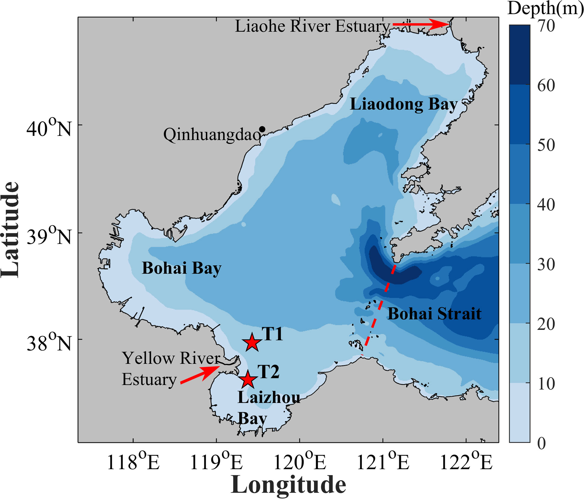
Figure 1 Topography of the model domain. Red stars indicate the in-situ observation stations (T1, T2) for validating the model simulated surface currents.

2.2 Model validation

Tides, sea surface temperature (SST), and temperature fronts simulated by the ROMS model are validated with in-situ and satellite observations to evaluate the accuracy of the model results.

Tidal harmonic analysis of the simulated water level in 2016 is conducted by t-tide toolbox to obtain the co-tidal charts of the main tidal constituents M₂ and K₁ in the Bohai Sea (Figure 2). The M₂ constituent has two amphidromic points located near the Yellow River estuary and Qinhuangdao, respectively. The K₁ constituent has one amphidromic point located in Bohai Strait. The amplitudes, phases, and amphidromic points are generally consistent with those in the Editorial Board for Marine Atlas, with small difference of the location of the amphidromic point for M₂ constituent (Chen and Editorial Board for Marine Atlas, 1993). The small difference is mainly attributed to the changes of the bathymetry induced by sea reclamation and sea level rise in recent years (Wei et al., 2020).

FIGURE 2

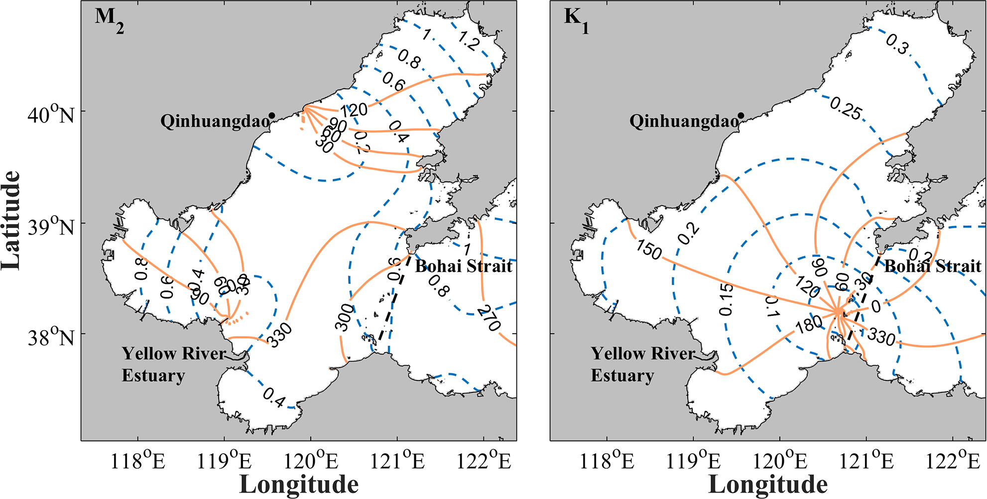
Figure 2 Co-tidal charts of the M₂ and K₁ constituents in the Bohai Sea. Blue dashed and orange solid lines indicate the tidal amplitudes (m) and phases (°), respectively.

Surface currents are further validated against the in-situ observed data at Stations T1 and T2 (Yu et al., 2021). The time of the observations is from 19:00 on June 5 to 20:00 on June 6, 2016. The results show that the model simulated surface velocities have conspicuous characteristics of semidiurnal tide and are almost consistent in magnitudes and directions with the observations (Figure 3). The formula of skill proposed by Wilmott (1981), previously applied in the validations of many numerical simulations (e.g., Warner et al., 2005; Ralston et al., 2010) is applied to evaluate the consistency between the observed and model simulated currents. The skill is calculated by

FIGURE 3

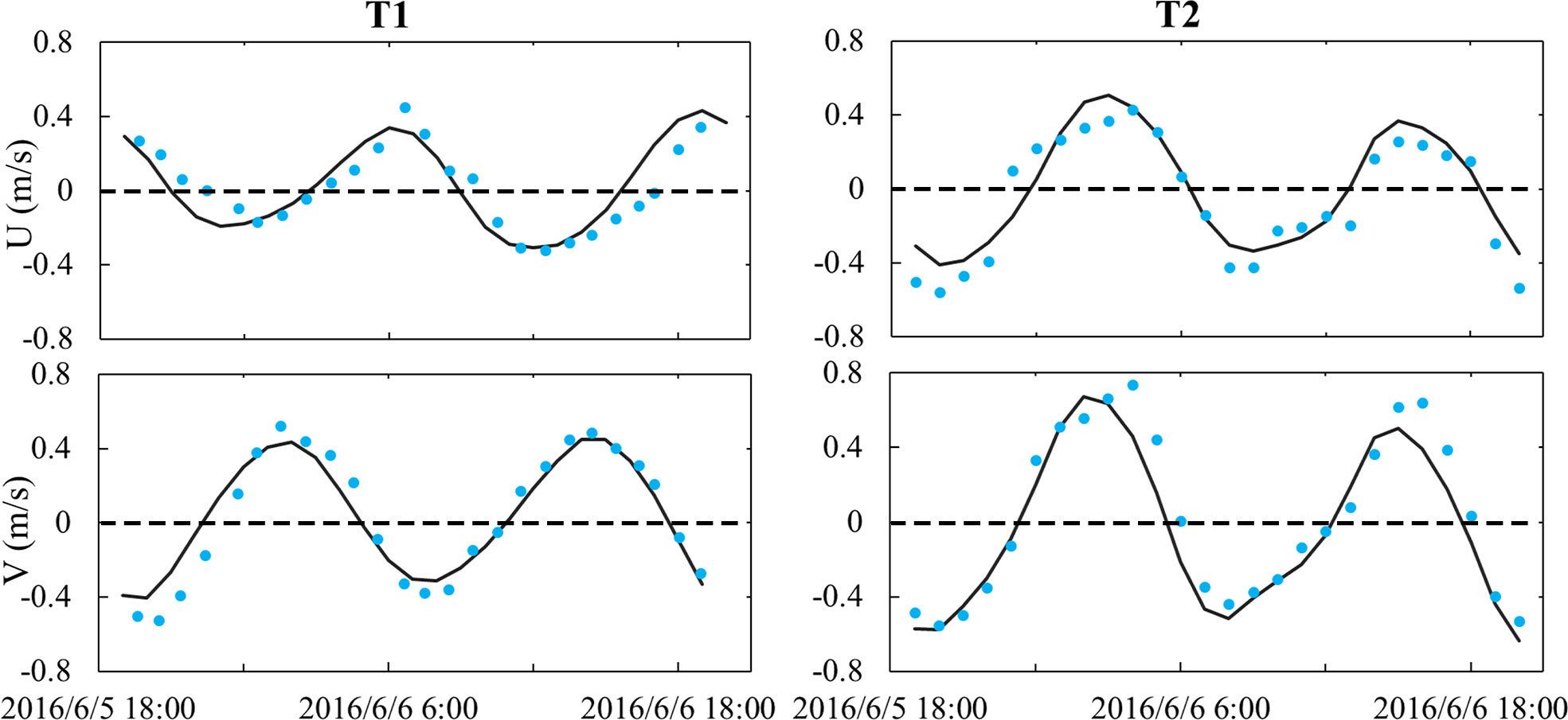
Figure 3 Validation of surface currents at Stations T1 and T2. Black solid lines and blue dots indicate the model simulated and in-situ observed results, respectively. Positive values indicate eastward or northward directions.

$\begin{array}{ll}\mathit{\text{ skill}}=\mathbf{1}-\frac{{\sum }_{\mathit{\text{i}}=1}^{\mathit{\text{N}}}{\left({\mathit{\text{M}}}_{\mathit{\text{i}}}-{\mathit{\text{O}}}_{\mathit{\text{i}}}\right)}^2}{{\sum }_{\mathit{\text{i}}=1}^{\mathit{\text{N}}}{\left(\left|{\mathit{\text{M}}}_{\mathit{\text{i}}}-\overline{{\mathit{\text{O}}}_{\mathit{\text{i}}}}\right|+\left|{\mathit{\text{O}}}_{\mathit{\text{i}}}-\overline{{\mathit{\text{O}}}_{\mathit{\text{i}}}}\right|\right)}^2}& (1)\end{array}$

where M_i and O_i indicate the model and observation results, respectively. Overbar indicates time mean. Perfect agreement between model results and observations yields a skill of one and complete disagreement yields a skill of zero. The skills of U and V are all around 0.9 at both stations, which indicate that the simulated results are in agreement with the observations.

Frontogenesis is one primary mechanism for the generation of submesoscale motions. To validate the model simulated fronts, the horizontal SST gradient |∇_hT| and frontal probability are calculated to compare with the satellite observed results. Daily MODIS-Aqua Level-3 SST data (https://oceancolor.gsfc.nasa.gov/) with a 4-km spatial resolution are employed for verifying the modeled SST fronts. Although there are missing data in some Level-3 products due to clouds, the available SST data are applicable to study the SST fronts (Castelao and Wang, 2014; Wang et al., 2015). For comparison, the modeled SST are daily and spatially averaged in 4-km windows before calculating |∇_hT| and frontal probability. The horizontal SST gradient |∇_hT| is calculated at each grid based on all daily remote sensing and modeled SST in 2016. In the present study, the regions with |∇_hT|> 5 x 10^-5 ° C/m are defined as SST fronts. We take the number of days a grid quantified as a front, and divide this value by the days that there is a valid value at the grid in the whole year of 2016, yielding a probability of detecting a front.

As shown in Figure 4, the modeled annually averaged |∇_hT| and frontal probability are both consistent with the results from the satellite data. The small difference between the model and satellite results is perhaps partly attributed to the higher model resolution (~500 m) than MODIS-Aqua Level-3 SST product (~4 km), so stronger fronts, especially submesoscale fronts, can be better resolved by numerical model, leading to higher |∇_hT| and frontal probability. We also have attempted to set other thresholds to compute the frontal probability, such as 8 x 10^-5 °C/m and 1 x 10^-4 °C/m, and the results show that the numerical simulation is consistent with the satellite data (not shown for brevity). Although the 4-km satellite products could not resolve submesoscale structures well enough, the consistence between the model simulated and satellite observed SST fronts proves the capabilities of the model to depict the general spatio-temporal distribution of SST fronts.

FIGURE 4

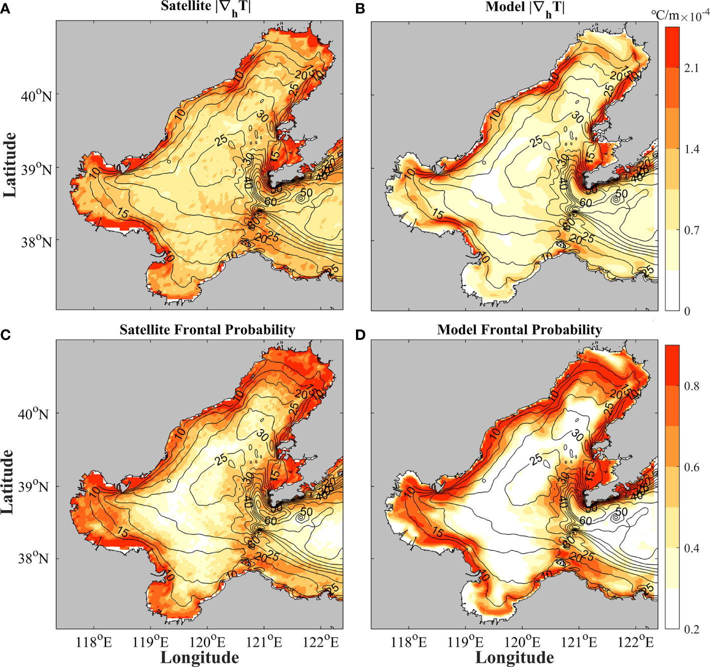
Figure 4 Annually averaged |∇_hT| and frontal probability quantified with the (A, C) satellite and (B, D) model data. Black contours indicate isobaths (m) with an interval of 5 m.

Furthermore, the instantaneous satellite images of SST and ocean color with a higher resolution (~1 km) (https://optics.marine.usf.edu) are compared with the simulation results. Affected by frequent cloud cover, there are many missing values in the instantaneous satellite images. Some snapshots with good coverage are selected to compare with the model results. Two examples are presented in Figure 5. The model simulated horizontal distribution of SST (Figure 5A) is roughly identical to the satellite result (Figure 5B), including the features of the cold waters in the east of the Bohai Bay, the south of the Liaodong Bay, and near the Bohai Strait. The abrupt spatial changes of SST are corresponding to fronts, which are often corresponding to the clear boundaries of water color. The waters with abrupt SST changes in the model results (Figure 5C) resemble the satellite water color image (Figure 5D), demonstrating the good performance of the model in simulating the horizontal characteristics of SST and fronts in the Bohai Sea. The images in other days give similar results (not shown for brevity).

FIGURE 5

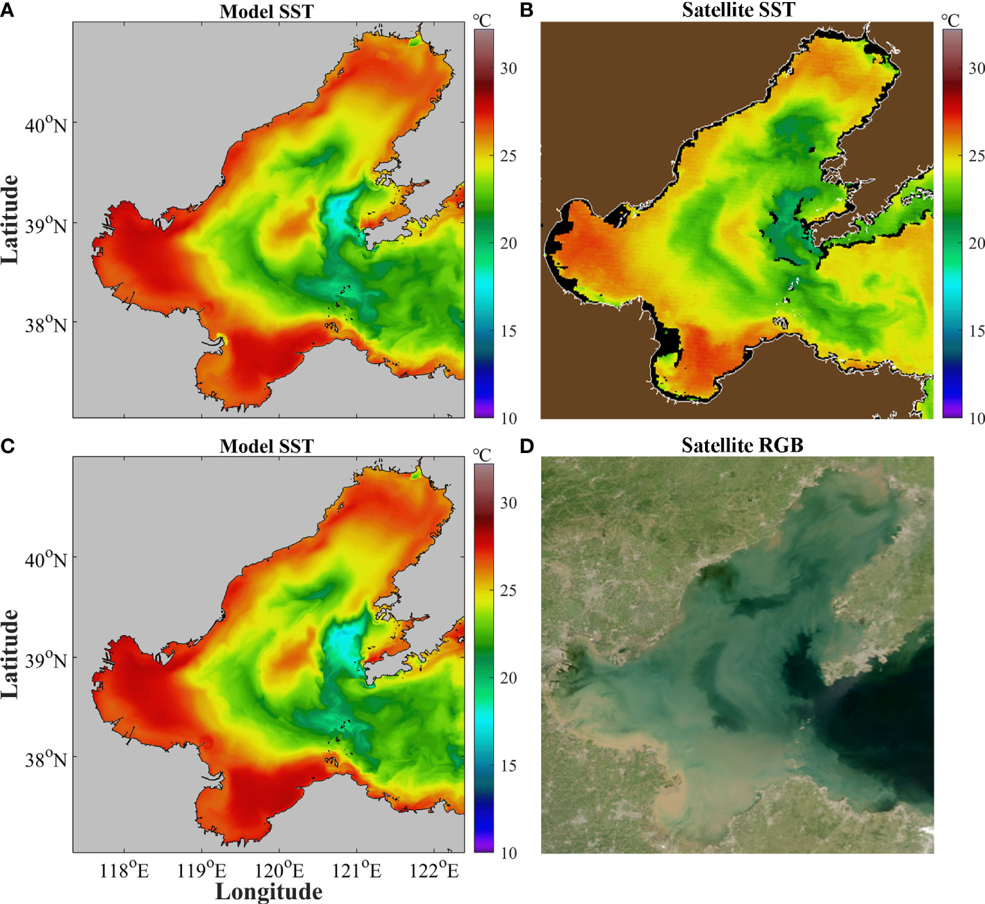
Figure 5 Comparison between the model and satellite images. (A) Model simulated SST at 17:00 on August 26, 2016; (B) Satellite observed SST at 17:25 on August 26, 2016; (C) Model simulated SST at 5:00 on August 26, 2016; (D) Satellite observed Red-Green-Blue (RGB) true-color composite image at 5:25 on August 26, 2016. The satellite images are from the Optical Oceanography Lab in University of South Florida. The RGB map in (D) is from normalized water-leaving radiance at 547 nm (R), 488 nm (G), and 443 nm (B) images, and is used to identify various ocean water types, from shallow (bright), sediment-rich (brownish), phytoplankton-rich (darkish), CDOM-rich (colored dissolved organic matter) (darkish), to blue waters (bluish) (Hu et al., 2005).

In the present study, we mainly focus on surface fronts, so SST and ocean color are used to validate the model results. We do not validate sea surface salinity (SSS), although it also has effects on the density (buoyancy) fronts. One reason is that there is no high-resolution satellite observed SSS. The other reason is that in most regions of the Bohai Sea, surface density fronts are mainly controlled by SST, as shown in the following analysis.

According to Barkan et al. (2017), Turner angle (Tu) is calculated to investigate the T–S relations based on the model results. The formula is as follows:

$\begin{array}{ll}{\mathit{\text{R}}}_{\mathit{\text{x}}}\mathit{=}\frac{\mathit{\text{α}}\mathit{\partial }\mathit{\text{T}}/\mathit{\partial }\mathit{\text{x}}}{\mathit{\text{β}}\mathit{\partial }\mathit{\text{S}}/\mathit{\partial }\mathit{\text{x}}}\mathit{,} {\mathit{\text{R}}}_{\mathit{\text{y}}}\mathit{=}\frac{\mathit{\text{α}}\mathit{\partial }\mathit{\text{T}}/\mathit{\partial }\mathit{\text{y}}}{\mathit{\text{β}}\mathit{\partial }\mathit{\text{S}}/\mathit{\partial }\mathit{\text{y}}}& (2)\end{array}$

$\begin{array}{ll}{\mathit{\text{Tu}}}_{\mathit{\text{x}}}\mathit{=}\mathit{\text{arctan}}\left({\mathit{\text{R}}}_{\mathit{\text{x}}}\right){\mathit{\text{, Tu}}}_{\mathit{\text{y}}}\mathit{=}\mathit{\text{arctan}}\left({\mathit{\text{R}}}_{\mathit{\text{y}}}\right)& (3)\end{array}$

where α and β are the expansion and contraction coefficients of potential temperature (T) and salinity (S). Turner angles values in the range (0<|Tu|<π/4) represent salinity dominated, and values in the range (π/4<|Tu|< π/2) represent regions where temperature is dominated. It is found that the value and distribution of Tu_x and Tu_y are highly consistent (not shown for brevity). Two examples of Tu_x in winter and summer are shown in Figure 6. The relatively small values of Tu_x in the bays (Figure 6) indicate that salinity is an important factor, which is mainly due to the influence of the river outflows. However, the values of Tu_x in most of the Bohai Sea are greater than π/4 (Figure 6), indicating that temperature generally dominated. In addition, the locations of SSS fronts are usually aligned with SST fronts (Wang et al., 2021b). Therefore, it is reasonable to verify that the model results and fronts by temperature (Figures 4, 5).

FIGURE 6

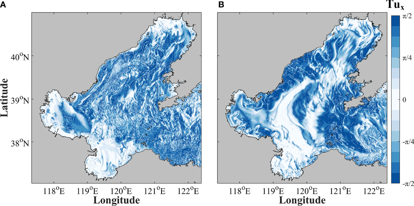
Figure 6 Model simulated Tu_x at (A) 12:00 on July 20, 2016, and (B) 12:00 on December 20, 2016.

3 Results

3.1 Spatial distribution of submesoscale motions

Submesoscale motions are often featured with strong vertical vorticity ζ=v_x−u_y (ζ/f ~1), horizontal divergence δ = u_x + v_y, horizontal velocity gradient $\left|{\nabla }_{h}U\right|=\sqrt{u_x^2+v_x^2+u_y^2+v_y^2}$, and horizontal buoyancy gradient $\left|{\nabla }_{h}b\right|=\sqrt{b_x^2+b_y^2}$, where (u, v) are the horizontal velocity components in the (eastward, northward) directions; subscripts (x, y) indicate horizontal derivatives; $b=-g\frac{\rho }{{\rho }_0}$ is the buoyancy. Snapshots of these indicators in the Bohai Sea at the corresponding time of Figure 5C are shown in Figure 7.

FIGURE 7

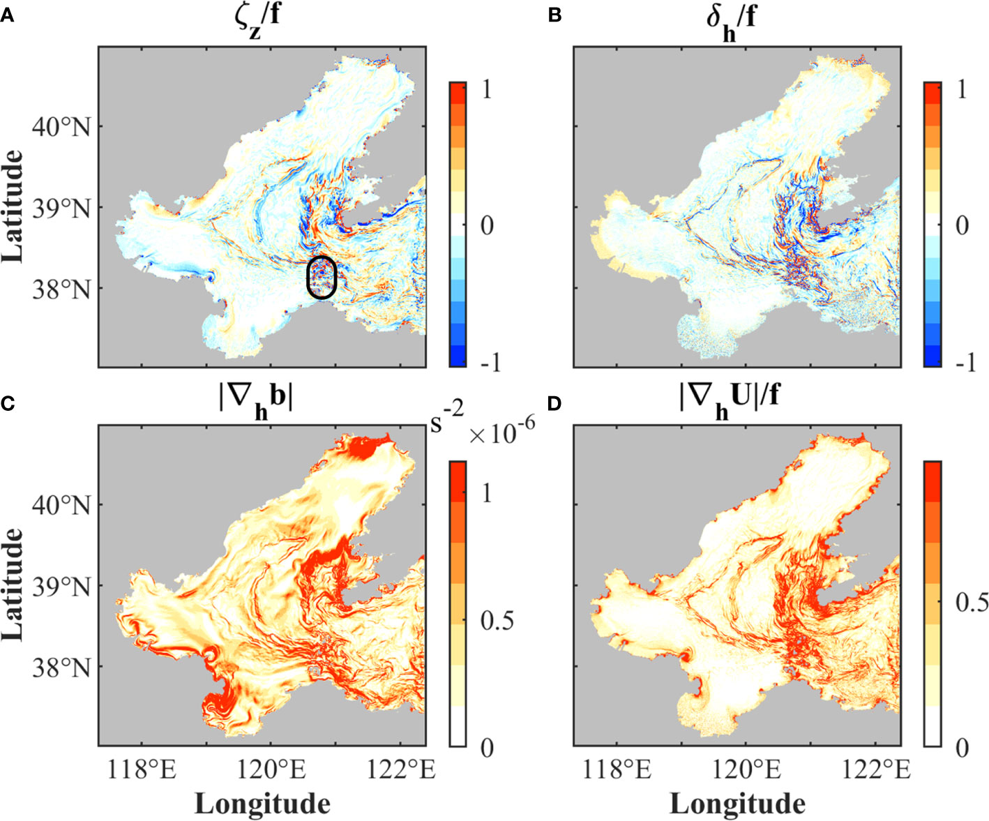
Figure 7 Instantaneous fields of (A) vertical vorticity normalized by the Coriolis frequency ζ/f , (B) divergence normalized by the Coriolis frequency δ/f, (C) absolute value of horizontal buoyancy gradient |∇_hb|, and (D) absolute value of horizontal velocity gradient normalized by the Coriolis frequency |∇_hU|/f, at the corresponding time of Figure 5C. The black ellipse in (A) indicates the region with a few islands.

The spatial distributions of the submesoscale indicators are roughly consistent with each other. Shallow coastal waters, the Bohai Strait, and the areas around islands exhibit more active submesoscale motions than other regions (Figure 7). High values of the submesoscale indicators are also found in the central area of the Bohai Sea due to the intrusion of cold water (Figure 5C). These high-value areas are primarily along isobaths, and resemble the sharp changes of water color (Figure 5D). Submesoscale motions near the Yellow River and Liaohe River estuaries differ from most of the other submesoscale processes in their higher magnitude of |∇_hb|. This is mainly associated with the river outflow, resulting in large horizontal salinity and buoyancy gradients, and complex frontal structures.

The submesoscale motions in the Bohai Sea are potentially affected by multiple factors such as winds, bottom boundary layer, river discharge, and tidal currents, hence resulting in spatial and temporal variabilities. To investigate the spatial and temporal characteristics of the submesoscale motions in a whole year, we calculate the temporal root-mean-square (RMS) and spatial RMS values of the submesoscale indicators (ζ, δ, |∇_hb|, and |∇_hU|), respectively.

The temporal RMS values of submesoscale indicators (ζ, δ, |∇_hb|, and |∇_hU|) at each grid cell (901 x 910 grids in total) are calculated using instantaneous model outputs at 1-hour intervals in the whole year of 2016 (8784 time points in total). Although the locations and intensities of the submesoscale motions vary with time under the effects of tidal currents, bathymetry, monsoons, and so on, there are some general spatial characteristics. According to the spatial distributions of the temporal RMS (Figure 8), during most time in one year, submesoscale motions are pervasively distributed in the shallow coastal waters, near the estuaries, the Bohai Strait, and the areas around islands, corresponding to the instantaneous features shown in Figure 7.

FIGURE 8

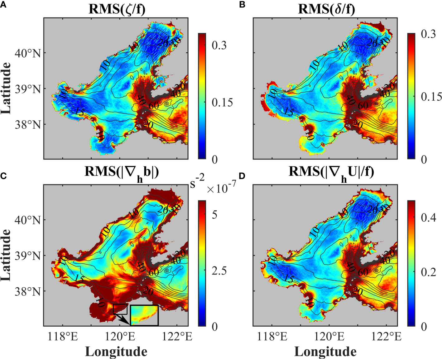
Figure 8 Temporal RMS of surface (A) ζ/f , (B) δ/f , (C) |∇_hb|, and (D) |∇_hU|/f. Black contours indicate isobaths (m) with an interval of 5 m. The subplot in the bottom of panel (C) indicates the temporal RMS of |∇_hb| inside the black box with the color bar range of 0 to 1.2 x 10^-6 s^-2. The subplot is used to show that the nearshore fronts tend to be parallel to the coast.

In the regions with sharp changes of water depth, such as the northern Bohai Bay, the east and west sides of the Liaodong Bay, and the northern Bohai Strait, the temporal RMS values are significantly high. It is consistent with the frontal probability (Figure 4D), indicating the high occurrence probability of submesoscale motions in these regions all year round. The magnitude of |∇_hb| near the estuarine mouths is much larger than the other areas due to the effects of freshwater from the rivers, but the along-coast frontal structure is perspicuous after changing the range of color bar (bottom subplot in Figure 8C). The strain field induced by the complex topography can promote the formation and development of the submesoscale motions, so there are high RMS values of ζ, δ, |∇_hb|, and |∇_hU| in the regions nearby the Bohai Strait and islands. Therefore, compared with the central region of the Bohai Sea, submesoscale motions are more ubiquitous and complex near the Bohai Strait.

3.2 Temporal variations of submesoscale motions

To investigate the temporal variations of submesoscale motions, the spatial RMS values of submesoscale indicators (ζ, δ, |∇_hb|, and |∇_hU|) at each moment (8784 time points in 2016) are calculated (Figure 9). The spatial RMS values of horizontal strain rate $S=\sqrt{u_x^2+v_y^2+\frac{1}{2}{\left(u_y+v_x\right)}^2}$ and surface kinetic energy KE=ρ(u²+v²)∕2 are also calculated to study their relationships with submesoscale motions. To eliminate the influences of the open boundaries, the regions on the east of 122°E are removed when calculating the spatial RMS values.

FIGURE 9

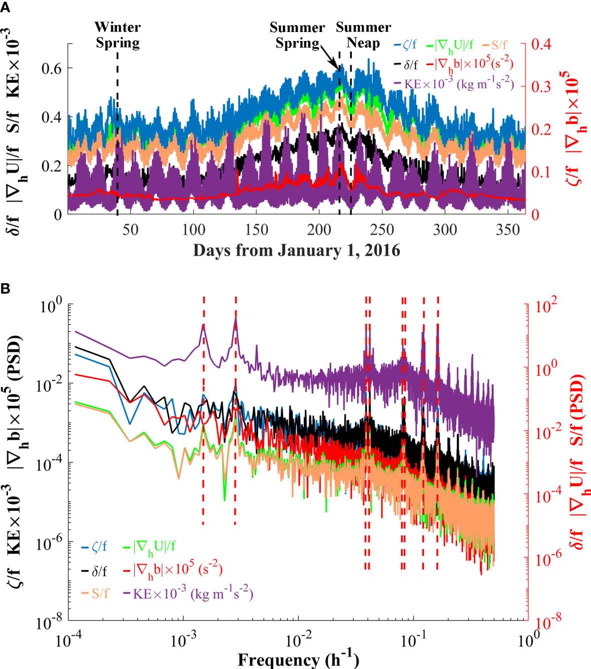
Figure 9 (A) Time series and (B) power spectra of the spatial RMS values of surface ζ/f, δ/f, |∇_hb|, |∇_hU/f|, S/f, and KE in 2016. Vertical dashed black lines in (A) represent the corresponding time of the cases in maximum spring and minimum neap tides in summer, and maximum spring tide in winter shown in Figures 10‐14. Vertical dashed red lines in (B) indicate the locations of peaks.

The submesoscale indicators (ζ, δ, and |∇_hU|) almost exhibit the same temporal variability as horizontal strain and KE (Figure 9A). The peaks at 28 and 14.5 days and 25.8, 23.9, 12.4, 12, 8.2, and 6.2 hours shown in the power spectra (Figure 9B) are consistent with the periods or double of the periods of the main tidal constituents in the Bohai Sea (e.g., spring-neap, O₁, K₁, M₂, S₂, M₃, and M₄). Those indicate that tides are significant controlling factors of the temporal variations of submesoscale motions in the Bohai Sea. The spring-neap tide cycle is the most apparent feature of the temporal variations of the submesoscale motions (Figure 9A). River outflow leads to strong horizontal buoyancy gradients near the estuaries during most time (Figure 8C), which has significant effects on the spatial RMS values, so |∇_hb| shows less obvious periodical variation compared with the other submesoscale indicators (Figure 9A). Nevertheless, the horizontal buoyancy gradient |∇_hb| also has the variation with a period of 14.6 days (Figure 9B). In addition to the tidal cycles, seasonal variations are also apparent in the spatial RMS values of submesoscale motions, with the highest in summer. The spatial RMS values increase in spring and reach the maximum in early August, indicating that the submesoscale motions in the Bohai Sea are more active in summer.

4 Discussion

As described in Section 3, the submesoscale motions in the Bohai Sea have significant spatial, spring-neap and seasonal variabilities. To explain these variabilities, the generation mechanisms and dominant factors of the submesoscale motions are analyzed in this section.

4.1 Mechanisms for the generation of vorticity

Based on time series of the spatial RMS values (Figure 9A), we selected three cases to explain the spring-neap and winter-summer variabilities of the submesoscale motions. Cases during the other periods give similar results (not shown for brevity). To get more detailed information about the spatial, spring-neap, and summer-winter variations of submesoscale processes, the instantaneous fields of submesoscale indicators (ζ, δ, |∇_hb|, and |∇_hU|) from three cases are presented in Figure 10. The results illustrate that the submesoscale indicators in spring tides in summer are enhanced in general compared with the neap tides. In spring tides, there are active submesoscale motions in the central area of the Bohai Sea, the Bohai Strait, and the northern Laizhou Bay. During spring tides in winter, submesoscale motions are even less active than neap tides in summer. The results during other tidal cycles in 2016 also resemble those shown in Figure 10.

FIGURE 10

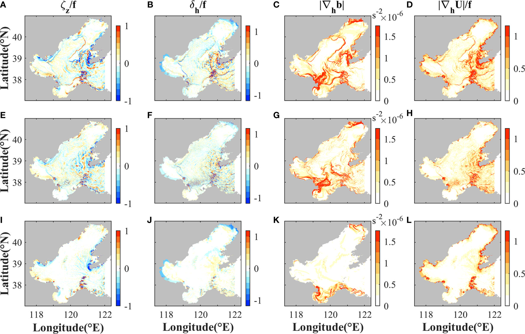
Figure 10 Distributions of the submesoscale indicators (A, E, I) ζ/f, (B, F, J) δ/f, (C, G, K) |∇_hb|, and (D, H, L) |∇_hU/f| during (top) maximum spring tide and (middle) minimum neap tide in summer, and (bottom) maximum spring tide in winter. The corresponding time is noted in Figure 9A. These snapshots are chosen at the time with maximum KE in the corresponding tidal cycles.

One fundamental feature of the submesoscale processes is that they have vertical vorticities those are close to f. To study how the high vertical vorticities are generated, we calculated the terms in the vertical vorticity equation based on the model output data. The vertical vorticity equation can be obtained by taking the curls of the horizontal momentum equations and expressed by:

$\begin{array}{ll}\frac{\text{Dζ}}{D\text{t}}=\underset{F_{div}}{\underbrace{-\left(\text{ζ}+\mathit{f}\right)\delta }}+\underset{F_{mix}}{\underbrace{\left[\frac{\partial }{\partial x}\frac{\partial }{\partial z}\left(A\frac{\partial v}{\partial z}\right)-\frac{\partial }{\partial y}\frac{\partial }{\partial z}\left(A\frac{\partial u}{\partial z}\right)\right]}}+\underset{F_{tilt}}{\underbrace{\left(\frac{\partial w}{\partial y}\frac{\partial u}{\partial z}-\frac{\partial w}{\partial x}\frac{\partial v}{\partial z}\right)}}\underset{F_{pres}}{\underbrace{-\left[\frac{\partial }{\partial x}\left(\frac{1}{\rho }\frac{\partial P}{\partial y}\right)-\frac{\partial }{\partial y}\left(\frac{1}{\rho }\frac{\partial P}{\partial x}\right)\right]}}& (4)\end{array}$

where ζ=v_x−u_y is vertical vorticity; (u, v, w) are the components of velocity in the three-dimensional field; f indicates the Coriolis frequency; p and p are the pressure and density, respectively; A is the parameterized vertical viscosity. The left term indicates the rate of change of the relative vorticity following a water parcel. All right terms represent the processes that generate or dissipate the relative vorticity, that is, the sources and sinks of the relative vorticity. The first term on the right F_div indicates the effect of horizontal divergence δ . The second term F_mix describes the role of vertical mixing. The third term F_tilt, often called as the tilting term, describes the influence of a horizontal gradient of vertical velocity in transforming vorticity from a horizontal direction to vertical direction. The last term F_pres represents the generation of vorticity by pressure gradient. Based on the model output, the magnitudes of the right terms are calculated to quantify their contributions to the change of vertical vorticity (Figure 11). The terms F_div and F_mix are found to be much larger than F_tilt and F_pres in the Bohai Sea (not shown for brevity), so the horizontal divergence and vertical mixing terms are dominant in generating or dissipating relative vorticity.

FIGURE 11

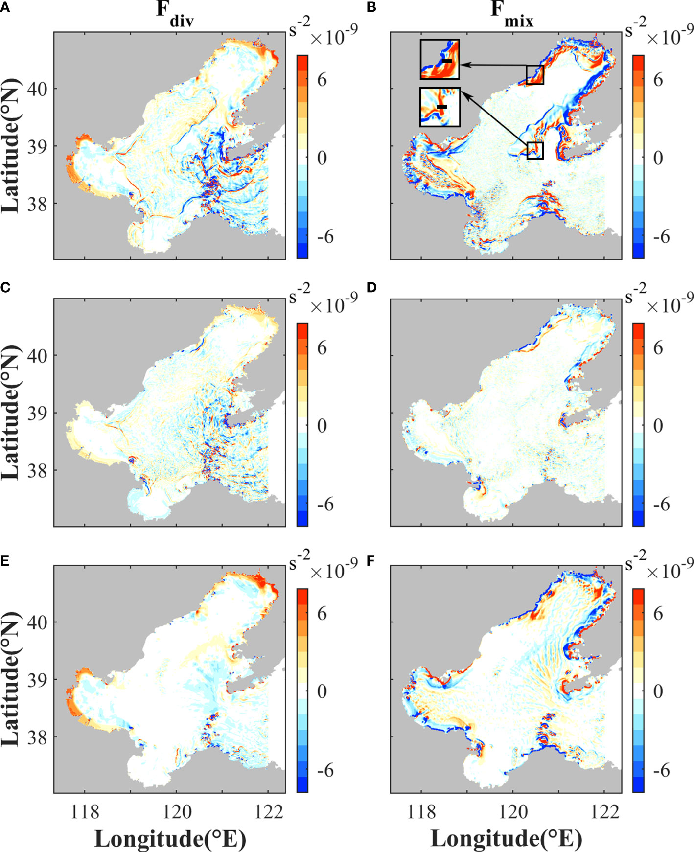
Figure 11 Magnitudes of (A, C, E) F_div and (B, D, F) F_mix in Eq. (4) during (top) maximum spring tide and (middle) minimum neap tide in summer, and (bottom) maximum spring tide in winter. The time is the same as Figure 10. The subplots are used to show the locations of sections in Figure 12.

The distributions of the divergence term F_div coincide with vorticity and divergence (Figure 10). Strong divergence or convergence tends to occur in frontal regions (Figure 10) (Barkan et al., 2019). Therefore, compared with neap tides, the divergence term F_div is stronger during spring tides in summer due to more and stronger submesoscale fronts being generated. In winter, submesoscale fronts are much less active than summer, hence F_div is small. In addition to F_div, the curl of vertical mixing F_mix is also a primary source for vertical vorticity. As shown in Figure 11, the magnitude of F_mix is comparable to F_div. During spring tides, large magnitude of F_mix mainly occurs in the regions with sharp changes of depth and behind headlands and islands.

In shallow waters, the sources of vertical mixing may come from surface and bottom frictions. The regions with large magnitude of F_mix are generally near the coasts (Figure 11), where water depth is less than 30 m. To explore the mechanisms for F_mix, two typical cross-front sections during maximum spring tide in summer are selected to study the vertical variation of shear stress. The magnitude of shear stress is calculated by $\tau =A\sqrt{{\left(\frac{\partial u}{\partial z}\right)}^2+{\left(\frac{\partial v}{\partial z}\right)}^2}$, where A indicates the vertical viscosity. As shown in Figure 12, shear stresses on both sides of the fronts decrease monotonically from bottom to surface, indicating that bottom friction dominates in the vertical mixing. Wind-induced friction does not dominate because there is no local maximum of shear stress at surface.

FIGURE 12

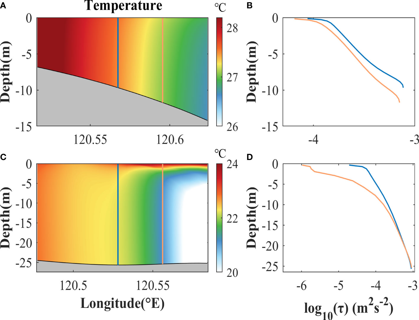
Figure 12 (A, B) Instantaneous fields of temperature and profiles of shear stresses in a cross-front section in the coastal area of the Liaodong Bay during maximum spring tide in summer. (C, D) as (A, B), but indicate the results in a cross-front section in the central of the Bohai Sea. The locations of the profiles in (B, D) are corresponding to the blue and orange lines in (A, C), respectively. The time is the same as the top panels of Figure 10. The locations of the vertical sections are shown as the black lines in the subplots of Figure 11B, respectively.

Across the front in the coastal area of the Liaodong Bay, temperature is almost homogeneous vertically (Figures 12A, B). The horizontal gradient of shear stress near surface is mainly due to the change of water depth across the front. In the central of the Bohai Sea, there is no apparent change of water depth across the front (Figure 12C, D). However, water is strongly stratified in the eastern side and almost homogeneous in the western side. The strong stratification in the eastern side inhibits vertical propagation of the bottom shear stress, hence resulting in much smaller stress near surface than the western side. In both cases shown in Figure 12, the horizontal change of the near-surface shear stress across the fronts leads to the curl of vertical mixing, hence inducing vertical vorticity. Other sections across the fronts with large magnitudes of F_mix show similar results (not shown for brevity).

Therefore, bottom friction has an important effect on vorticity due to the limited water depth in coastal seas. The curl of bottom shear stress is related to the change of water depth near the coasts (O’Donnell, 2010; Wang et al., 2022), so the distribution of F_mix is related to the topographic changes to some extent. This is unlike the situation in the deep water regions, where surface friction induced by winds is generally more important than bottom friction for the generation of surface submesoscale motions (McWilliams et al., 2015).

During spring tides, the magnitude and curl of bottom stress are large due to strong tidal velocity. Thus, F_mix is strong to generate high vorticity in the regions with sharp changes of depth and behind headlands and islands. Once generated, high vorticities and fronts would be advected under the effects of background tidal currents. Due to the strong divergence and convergence in frontal regions, F_div also plays a primary role for further evolution of vorticity. After vorticity and fronts are advected away from the regions with sharp topographic changes, F_mix is no longer as important as F_div. This is why F_mix does not coincide with vorticity in the central Bohai Sea. During neap tides, due to weak tidal currents, the curl of vertical mixing is smaller than spring tides, so submesoscale motions are less active.

As for the seasonal variation, although the curl of bottom stress and vertical mixing are high during spring tides in winter, the magnitudes of F_div are much smaller than that in summer, so vorticities are much less active. Because F_div is related to fronts (McWilliams, 2016; Wang et al., 2021b), frontogenesis is analyzed in the following to study the mechanisms for the seasonal variation.

4.2 Frontogenesis

As discussed above, submesoscale fronts are much less active in winter than summer, and this is the main reason for lower vorticity. Frontogenesis is associated with the evolution processes of horizontal buoyancy and velocity gradients (McWilliams, 2021; Wang et al., 2021b). In previous studies on submesoscale motions, the frontogenetic tendency equation for horizontal buoyancy gradients has been demonstrated to be informative for frontogenesis of submesoscale fronts and filaments (Gula et al., 2014; Barkan et al., 2019). To find out the reasons for seasonal variation of submesoscale structures and get further detailed information about the mechanism responsible for fronts, we calculate the terms in the Lagrangian frontogenetic tendency equation to study the sources and sinks of the horizontal buoyancy gradients. In the present study, the frontogenetic tendency equation for horizontal buoyancy gradient |∇_hb| is applied, which can be derived by taking horizontal derivatives of the tracer transport equations. The frontogenetic tendency equation for horizontal buoyancy gradient can be written as

$\begin{array}{ll}\frac{1}{2}\frac{D{\left|{\nabla }_{h}b\right|}^2}{Dt}=\underset{T_{adv}}{\underbrace{\left[-u_x{b}_x^2-v_y{b}_y^2-\left(u_y+v_x\right)b_x{b}_y\right]}}\underset{T_w}{\underbrace{-b_z{\nabla }_{h}w·{\nabla }_{h}b}}+\underset{T_{dv}}{\underbrace{{\nabla }_h\left[\frac{\partial }{\partial z}\left(K_z\frac{\partial b}{\partial z}\right)\right]·{\nabla }_{h}b}}+\underset{T_{dh}}{\underbrace{{\nabla }_h\left[D_h\right]·{\nabla }_{h}b}}& (5)\end{array}$

where $\frac{1}{2}\frac{\text{D}{\left|{\nabla }_{\text{h}}\text{b}\right|}^2}{\text{Dt}}$ indicates the time rate of change of horizontal buoyancy gradient in a Lagrangian reference frame (Gula et al., 2014). The right-side terms of the equation include horizontal advection term T_adv, vertical advection term T_w, vertical mixing term T_dv, and horizontal mixing term T_dh. The symbols (u, v, w) indicate the velocity components in the three-dimensional field; subscripts (x, y, z) indicate horizontal and vertical derivatives; K indicates parameterized vertical diffusivity; D_h indicates the horizontal buoyancy diffusion. Snapshots of the primary tendency terms are shown in Figure 13. It is found that horizontal mixing term T_dh is not dominant, so it is not shown.

FIGURE 13

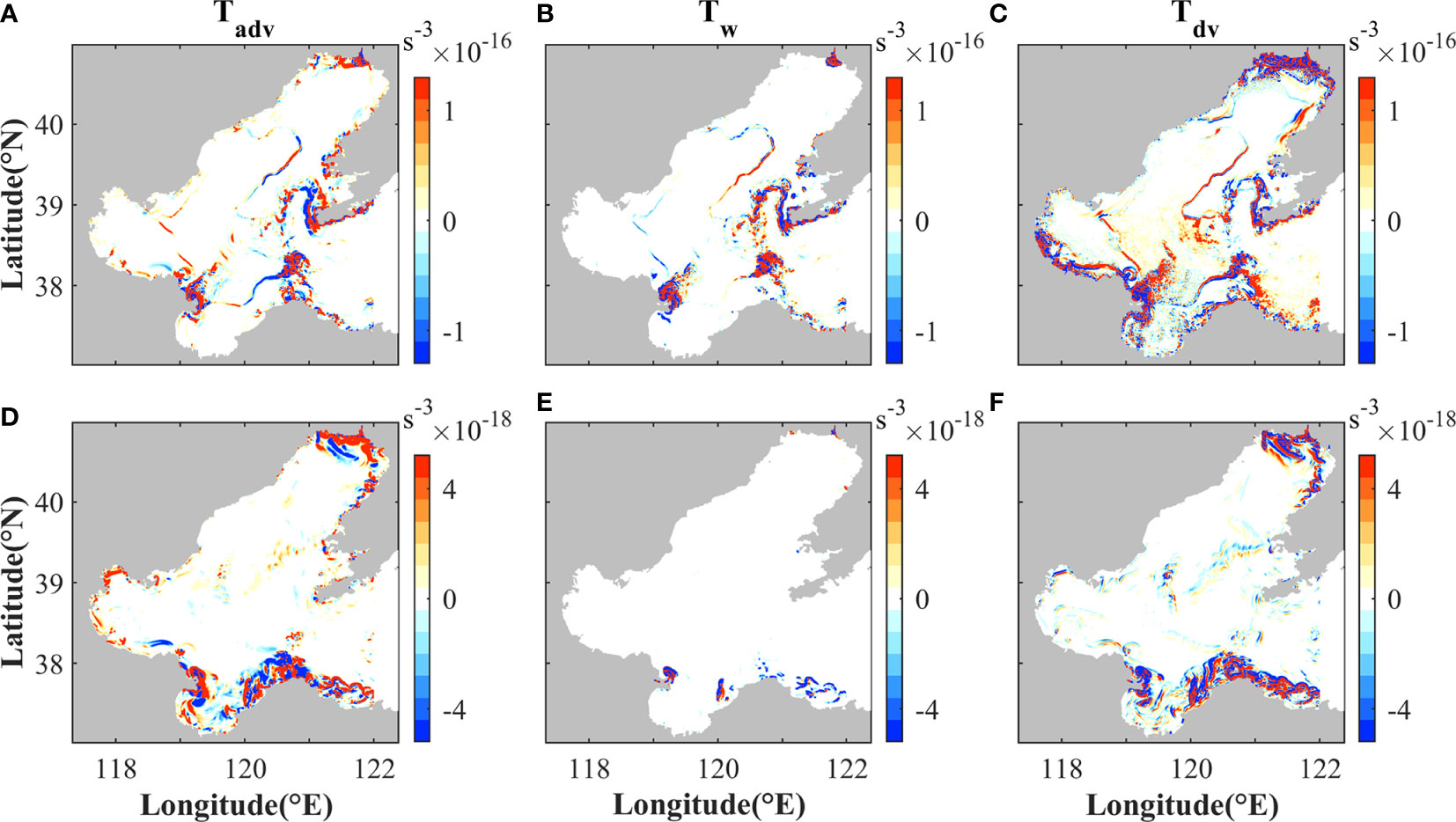
Figure 13 Magnitudes of the frontogenetic tendency terms (A, D) T_adv, (B, E) T_w, and (C, F) T_dv in Eq. (5) during (top) maximum spring tide in summer and (bottom) winter. The corresponding time is noted in Figure 9A.

The spatial distributions of the three tendency terms are basically consistent with the submesoscale indicators (Figure 10). Frontogenetic tendency terms near the estuaries are high due to high |∇_hb|. The tendency terms are much greater in summer than those in winter (Figure 13). All of the three terms could be positive or negative in different parts of the fronts (Figure 13), indicating that they could be frontogenetic or frontolytic. We account for the contributions of the three terms to frontogenesis, and find that their contributions are comparable during summer. While during winter, frontogenesis is mainly induced by the horizontal advection and vertical mixing terms near the coasts.

Horizontal advection term T_adv represents the effects of horizontal strain field on sharpening or weakening the preexisting horizontal buoyancy gradients. Although the convergence associated with secondary circulations plays a primary role in the horizontal strain field when fronts have been formed, horizontal velocity strain is generally induced by the deformation of background currents when fronts are triggered at early stage (Barkan et al., 2019; Wang et al., 2021b). Therefore, to induce T_adv at early stage, there should be preexisting background horizontal buoyancy gradients and deformation of background currents. Compared with winter, there is much more horizontal density variance in summer (Figure 14). This is mainly attributed to two reasons. First, the high river runoff induces high salinity and density variance near the river mouths in summer, while runoff is low during winter. Second, cold water intrudes into the central Bohai Sea from the Bohai Strait in summer (Figure 5), and induces high temperature and density variance in the Bohai Strait and central Bohai Sea. Therefore, although the strength of surface currents in winter is comparable to that in summer and the topography would induce strong flow deformation (Figure 14), fronts are easier to be triggered under the effects of T_adv in summer due to stronger background horizontal density variance. After fronts are generated, the convergence at fronts will have positive feedback to T_adv, resulting in further sharpening the fronts (Barkan et al., 2019; Wang et al., 2021b).

FIGURE 14

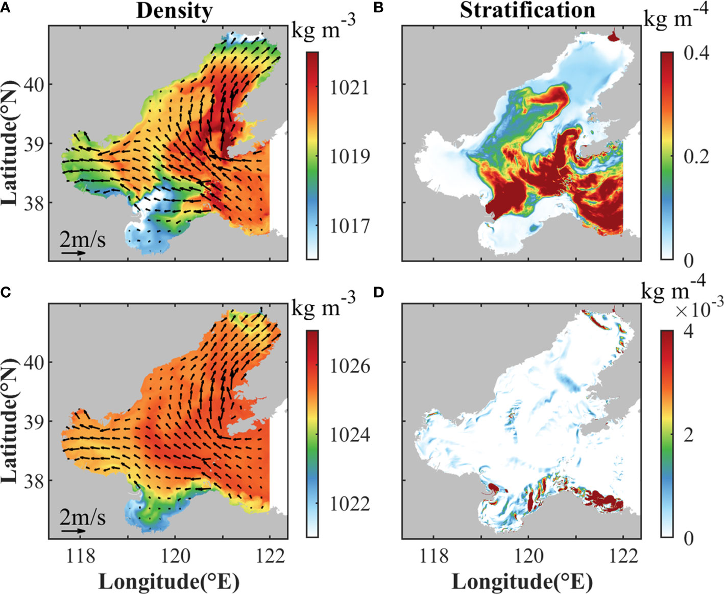
Figure 14 (A, C) Surface density and (B, D) stratification in the upper layer during (top) maximum spring tide in summer and (bottom) winter. The time is the same as Figure 13. The arrows in (A, C) indicate horizontal velocities in the upper layer. Stratification is quantified as the absolute value of vertical density gradient between surface and 5 m depth.

Vertical advection and mixing terms (T_w and T_dv) represent the effects of horizontal gradients of vertical velocity and mixing in transforming buoyancy gradient from a vertical direction to horizontal direction, respectively. Thus, vertical buoyancy (density) gradient is primary for inducing T_w and T_dv. As shown in Figures 14B, D, the vertical density gradient in summer is much stronger than that in winter, so it could provide more sources for inducing T_w and T_dv. In addition, the sharp horizontal changes of stratification in summer are mostly consistent with the regions where fronts occur, indicating the important roles of the vertical processes in frontogenesis.

As discussed above, strong background horizontal and vertical density gradients in summer provide favorable conditions for frontogenesis under the effects of T_adv, T_w, and T_dv. As fronts are generated and evolve, the convegence and divergence near fronts will have effects on the magnitude of vertical vorticity. Therefore, compared to winter, more and stronger fronts are generated in summer and induce stronger divergence term F_div for generating vertical vorticity.

5 Conclusions

In this study, a high-resolution numerical simulation is conducted to investigate the temporal and spatial characteristics of submesoscale motions in the Bohai Sea and explore their mechanisms.

The results reveal that submesoscale structures are mainly in the shallow coastal waters, the Bohai Strait, the regions near the islands and estuaries, and mostly tend to be parallel to the isobaths. These features agree well with the temperature gradient and frontal probability based on remote sensing data. Periodic variations of submesoscale motions are closely related to the periods or double of the periods of the main tidal constituents and spring-neap cycles in the Bohai Sea. The seasonal variations are also apparent, with more active submesoscale motions in summer.

One prominent feature of the submesoscale motions is that vertical vorticity is close to f. Through the vertical vorticity equation, it is found that the divergence and vertical mixing terms are primary sources for vertical vorticity. The curl of vertical mixing is large due to strong tidal velocity during spring tides in summer, resulting in more active submesoscale motions than neap tides. Despite of large curl of vertical mixing during spring tides in winter, the magnitudes of the divergence term are much smaller than that in summer. Based on the Lagrangian frontogenetic tendency equation, it is found that strong background horizontal and vertical density variance in summer provide more sources for inducing primary tendency terms, leading to more and stronger submesoscale fronts. The divergence and convergence near fronts enhance the magnitudes of vorticity. Therefore, compared to summer, submesoscale fronts are less active in winter.

Being different from the deep sea, tides and bottom friction are found to play important roles in the variability of submesoscale motions. The model horizontal resolution is 500 m, which is much larger than the water depth, so the hydrostatic approximation of the model is approximately valid for the submesoscale motions (Barkan et al., 2017). In future, it is of interest to explore the motions of finer spatial scales with nonhydrostatic models. With the increasing model resolutions, more detailed submesoscale processes are expected to be resolved. In this study, only the general characteristics and mechanisms of submesoscale motions in the Bohai Sea are investigated, while detailed analysis is not done for individual fronts or filaments. Further analysis will be conducted in the near future to show more detailed submesoscale dynamics in different local regions of the Bohai Sea.

Data availability statement

The raw data supporting the conclusions of this article will be made available by the authors, without undue reservation.

Author contributions

TW conceived the work. XS performed the model simulations. XS and TW conducted analyses and drafted the manuscript. YW gave input to the analysis process. All authors contributed to the article and approved the submitted version.

Funding

This study is supported by the National Natural Science Foundation of China (42076006) and the National Natural Science Foundation of China-Shandong Joint Fund (U2106204).

Acknowledgments

The authors thank Peng Zhao and Rui Li for providing the NEMO model outputs to build the open boundary conditions.

Conflict of interest

The authors declare that the research was conducted in the absence of any commercial or financial relationships that could be construed as a potential conflict of interest.

Publisher’s note

All claims expressed in this article are solely those of the authors and do not necessarily represent those of their affiliated organizations, or those of the publisher, the editors and the reviewers. Any product that may be evaluated in this article, or claim that may be made by its manufacturer, is not guaranteed or endorsed by the publisher.

References

Barkan R., McWilliams J. C., Molemaker J., Choi J., Srinivasan K., Shchepetkin A. F., et al. (2017). Submesoscale dynamics in the northern gulf of mexico. PartII: temperature-salinity relations and cross shelf transport processes. J. Phys. Oceanogr. 47, 2347–2361. doi: 10.1175/JPO-D-17-0040.1

CrossRef Full Text | Google Scholar

Barkan R., Molemaker M. J., Srinivasan K., McWilliams J. C., D’Asaro E. (2019). The role of horizontal divergence in submesoscale frontogenesis. J. Phys. Oceanogr. 49, 1593–1618. doi: 10.1175/JPO-D-18-0162.1

CrossRef Full Text | Google Scholar

Boccaletti G., Ferrari R., Fox-Kemper B. (2007). Mixed layer instabilities and restratification. J. Phys. Oceanogr. 37, 2228–2250. doi: 10.1175/JPO3101.1

CrossRef Full Text | Google Scholar

Callies J., Ferrari R., Klymak J. M., Gula J. (2015). Seasonality in submesoscale turbulence. Nat. Commun. 6, 1–8. doi: 10.1038/ncomms7862

CrossRef Full Text | Google Scholar

Capet X., McWilliams J. C., Molemaker M. J., Shchepetkin A. F. (2008). Mesoscale to submesoscale transition in the California current system. part III: Energy balance and flux. J. Phys. Oceanogr. 38, 2256–2269. doi: 10.1175/2008JPO3810.1

CrossRef Full Text | Google Scholar

Castelao R. M., Wang Y. (2014). Wind-driven variability in sea surface temperature front distribution in the California current system. J. Geophys. Res. Oceans 119, 1861–1875. doi: 10.1002/2013JC009531

CrossRef Full Text | Google Scholar

Chen D., Editorial Board for Marine Atlas (1993). Marine atlas of bohai Sea, yellow Sea and East China Sea (Hydrology) (Beijing: China Ocean Press).

Google Scholar

Choi B. H., Kim K. O., Eum H. M. (2002). Digital bathymetric and topographic data for neighboring seas of Korea. J. Korean Soc Coast. Ocean Eng. 14, 41–50.

Google Scholar

D'Asaro E. A. (1988). Generation of submesoscale vortices: A new mechanism. J. Geophys. Res. 93, 6685–6693. doi: 10.1029/JC093iC06p06685

CrossRef Full Text | Google Scholar

D'Asaro E. A., Shcherbina A. Y., Klymak J. M., Molemaker J., Novelli G., Guigand C. M., et al. (2018). Ocean convergence and the dispersion of flotsam. Proc. Natl. Acad. Sci. 115, 1162–1167. doi: 10.1073/pnas.1718453115

CrossRef Full Text | Google Scholar

Dauhajre D., McWilliams J. C. (2018). Diurnal evolution of submesoscale front and filament circulations. J. Phys. Ocean. 48, 2343–2361. doi: 10.1175/JPO-D-18-0143.1

CrossRef Full Text | Google Scholar

Dauhajre D. P., McWilliams J. C., Uchiyama Y. (2017). Submesoscale coherent structures on the continental shelf. J. Phys. Oceanogr. 47, 2949–2976. doi: 10.1175/JPO-D-16-0270.1

CrossRef Full Text | Google Scholar

Dong J., Fox-Kemper B., Zhang H., Dong C. (2020). The seasonality of submesoscale energy production, content, and cascade. Geophys. Res. Lett. 47, 2020GL087388. doi: 10.1029/2020GL087388

CrossRef Full Text | Google Scholar

Esposito G., Berta M., Centurioni L., Johnston H., Lodise G., Özgökmen T., et al. (2021). Submesoscale vorticity and divergence in the alboran Sea: Scale and depth dependence. Front. Mar. Sci. 8. doi: 10.3389/fmars.2021.678304

CrossRef Full Text | Google Scholar

Fairall C. W., Bradley E. F., Rogers D. P., Edson J. B., Young G. S. (1996). Bulk parameterization of air-sea fluxes for tropical ocean-global atmosphere coupled-ocean atmosphere response experiment. J. Geophys. Res. Oceans 101, 3747–3764. doi: 10.1029/95JC03205

CrossRef Full Text | Google Scholar

Fox-Kemper B., Ferrari R., Hallberg R. (2008). Parameterization of mixed layer eddies. part I: Theory and diagnosis. J. Phys. Oceanogr. 38, 1145–1165. doi: 10.1175/2007JPO3792.1

CrossRef Full Text | Google Scholar

Gula J., Molemaker M. J., McWilliams J. C. (2014). Submesoscale cold filaments in the gulf stream. J. Phys. Oceanogr. 44, 2617–2643. doi: 10.1175/JPO-D-14-0029.1

CrossRef Full Text | Google Scholar

Gula J., Molemaker M. J., McWilliams J. C. (2016). Topographic generation of submesoscale centrifugal instability and energy dissipation. Nat. Commun. 7, 12811. doi: 10.1038/ncomms12811

PubMed Abstract | CrossRef Full Text | Google Scholar

Hickox R., Belkin I., Cornilion P., Shan Z. (2000). Climatology and seasonal variability of ocean fronts in the East China, yellow and bohai seas from satellite SST data. Geophys. Res. Lett. 27, 2945–2948. doi: 10.1029/1999GL011223

CrossRef Full Text | Google Scholar

Hoskins B. J. (1982). The mathematical theory of frontogenesis. Annu. Rev. Fluid Mech. 14, 131–151. doi: 10.1146/annurev.fl.14.010182.001023

CrossRef Full Text | Google Scholar

Hu C., Muller-Karger F. E., Taylor C., Carder K. L., Kelble C., Johns E., et al. (2005). Red tide detection and tracing using MODIS fluorescence data: A regional example in SW Florida coastal waters. Remote Sens. Environ. 97, 311–321. doi: 10.1016/j.rse.2005.05.013

CrossRef Full Text | Google Scholar

Large W. G., McWilliams J. C., Doney S. C. (1994). Oceanic vertical mixing: A review and a model with a nonlocal boundary layer parameterization. Rev. Geophys. 32, 363–403. doi: 10.1029/94RG01872

CrossRef Full Text | Google Scholar

Lévy M., Franks P., Smith K. (2018). The role of submesoscale currents in structuring marine ecosystems. Nat. Commun. 9, 1–16. doi: 10.1038/s41467-018-07059-3

PubMed Abstract | CrossRef Full Text | Google Scholar

Lévy M., Klein P., Treguier A. (2001). Impact of sub-mesoscale physics on production and subduction of phytoplankton in an oligotrophic regime. J. Mar. Res. 59, 535–565. doi: 10.1357/002224001762842181

CrossRef Full Text | Google Scholar

Li X., Lorenz M., Klingbeil K., Chrysagi E., Gräwe U., Wu J., et al. (2022). Salinity mixing and diahaline exchange flow in a large multi-outlet estuary with islands. J. Phys. Oceanogr. 52, 2111–2127. doi: 10.1175/JPO-D-21-0292.1

CrossRef Full Text | Google Scholar

Li R., Lu Y., Hu X., Guo D., Zhao P., Wang N., et al. (2020). Space-time variations of sea ice in bohai Sea in the winter of 2009-2010 simulated with a coupled ocean and ice model. J. Oceanogr. 77, 243–258. doi: 10.1007/s10872-020-00566-2

CrossRef Full Text | Google Scholar

Liu G., Bracco A., Sitar A. (2021). Submesoscale mixing across the mixed layer in the gulf of Mexico. Front. Mar. Sci. 8. doi: 10.3389/fmars.2021.615066

CrossRef Full Text | Google Scholar

Li X., Yuan C., Li Y. (2013). Remote sensing monitoring and spatial-temporal variation of Bohai Bay coastal zone. Remote Sens. Land Resour. 25, 156–163. doi: 10.6046/gtzyyg.2013.02.26

CrossRef Full Text | Google Scholar

Mahadevan A. (2016). The impact of submesoscale physics on primary productivity of plankton. Annu. Rev. Mar. Sci. 8, 161–184. doi: 10.1146/annurev-marine-010814-015912

CrossRef Full Text | Google Scholar

McWilliams J. C. (2016). Submesoscale currents in the ocean. Proc. R. Soc A: Math. Phys. Eng. Sci. 472, 20160117. doi: 10.1098/rspa.2016.0117

CrossRef Full Text | Google Scholar

McWilliams J. C. (2021). Oceanic frontogenesis. Annu. Rev. Mar. Sci. 13, 227–253. doi: 10.1146/annurev-marine-032320-120725

CrossRef Full Text | Google Scholar

McWilliams J. C., Gula J., Molemaker M. J., Renault L., Shchepetkin A. F. (2015). Filament frontogenesis by boundary layer turbulence. J. Phys. Oceanogr. 45, 1988–2005. doi: 10.1175/JPO-D-14-0211.1

CrossRef Full Text | Google Scholar

McWilliams J. C., Molemaker M. J., Olafsdottir E. I. (2009). Linear fluctuation growth during frontogenesis. J. Phys. Oceanogr. 39, 3111–3129. doi: 10.1175/2009JPO4186.1

CrossRef Full Text | Google Scholar

O’Donnell J. (2010). “The dynamics of estuary plumes and fronts,” in Contemporary issues in estuarine physics. Ed. Levinson A. V. (Cambridge, UK: Cambridge University Press), 186–246. doi: 10.1017/CBO9780511676567.009

CrossRef Full Text | Google Scholar

Poje A. C., Özgökmen T. M., Lipphardt B. L. Jr., Haus B. K., Ryan E. H., Haza A. C., et al. (2014). Submesoscale dispersion in the vicinity of the deepwater horizon spill. Proc. Natl. Acad. Sci. 111, 12693–12698. doi: 10.1073/pnas.1402452111

CrossRef Full Text | Google Scholar

Ralston D. K., Geyer W. R., Lerczak J. A. (2010). Structure, variability, and salt flux in a strongly forced salt wedge estuary. J. Geophys. Res. 115, C06005. doi: 10.1029/2009JC005806

CrossRef Full Text | Google Scholar

Thomas L. N., Tandon A., Mahadevan A. (2008). Submesoscale processes and dynamics. Ocean Model. Eddy. Reg. 177, 17–38. doi: 10.1029/177GM04

CrossRef Full Text | Google Scholar

Wang T., Barkan R., McWilliams J. C., Molemaker M. J. (2021b). Structure of submesoscale fronts of the Mississippi river plume. J. Phys. Oceanogr. 51, 1113–1131. doi: 10.1175/JPO-D-20-0191.1

CrossRef Full Text | Google Scholar

Wang Y., Castelao R. M., Yuan Y. (2015). Seasonal variability of alongshore winds and sea surface temperature fronts in Eastern boundary current systems. J. Geophys. Res. Oceans 120, 2385–2400. doi: 10.1002/2014JC010379

CrossRef Full Text | Google Scholar

Wang T., Chai F., Xing X., Ning J., Jiang W. S., Riser S. (2021a). Influence of multi-scale dynamic on the nitrate distribution around the kuroshio extension: An investigation based on BGC-argo and satellite data. Prog. Oceanogr. 193, 102543. doi: 10.1016/j.pocean.2021.102543

CrossRef Full Text | Google Scholar

Wang T., Zhao S., Zhu L., McWilliams J. C., Galgani L., Amin R. M., et al. (2022). Accumulation, transformation and transport of microplastics in estuarine fronts. Nat. Rev. Earth Environ 3, 795-805. doi: 10.1038/s43017-022-00349-x

CrossRef Full Text | Google Scholar

Warner J. C., Geyer W. R., Lerczak J. A. (2005). Numerical modeling of an estuary: A comprehensive skill assessment. J. Geophys. Res. Oceans 110, C05001. doi: 10.1029/2004JC002691

CrossRef Full Text | Google Scholar

Wei H., Hainbucher D., Pohlmann T., Feng S., Suendermann J. (2004). Tidal-induced Lagrangian and eulerian mean circulation in the bohai Sea. J. Mar. Syst. 44, 141–151. doi: 10.1016/j.jmarsys.2003.09.007

CrossRef Full Text | Google Scholar

Wei H., Zhang H., Yang W., Feng J., Zhang C. (2020). “The changing bohai and yellow seas: a physical view,” in Changing Asia-pacific marginal seas. Eds. Chen C.-T. A., Guo X. (Singapore: Springer Singapore), 105–120. doi: 10.1007/978-981-15-4886-4_7

CrossRef Full Text | Google Scholar

Wilmott C. J. (1981). On the validation of models. Phys. Geogr. 2, 184–194. doi: 10.1080/02723646.1981.10642213

CrossRef Full Text | Google Scholar

Yu X., Guo X., Takeoka H. (2016). Fortnightly variation in the bottom thermal front and associated circulation in a semienclosed sea. J. Phys. Oceanogr. 46, 159–177. doi: 10.1175/JPO-D-15-0071.1

CrossRef Full Text | Google Scholar

Yu J., Zhang X., Feng Y., Jiang W., Deng F. (2021). Analysis of tidal-induced connectivity among coastal regions in the bohai Sea using the complex network theory. Estuar. Coast. Shelf Sci. 260, 107506. doi: 10.1016/j.ecss.2021.107506

CrossRef Full Text | Google Scholar

Zhan P., Guo D., Krokos G., Dong J., Duran R., Hoteit I. (2022). Submesoscale processes in the upper red Sea. J. Geophys. Res. Oceans 127, e2021JC018015. doi: 10.1029/2021JC018015

CrossRef Full Text | Google Scholar

Zhang G., Wei H., Xiao J., Zhang H., Li Z. (2020). Variation of tidal front position in liaodong bay during summer 2017. Oceanol. Limnol. Sin. 51, 1–12. doi: 10.11693/hyhz20190600110

CrossRef Full Text | Google Scholar

Zhao B., Cao D., Li W., Wang Q. (2001). Tidal mixing characters and tidal fronts phenomenons in the Bohai Sea. Acta Oceanol. Sin. 23, 113–120. doi: 10.3321/j.issn:0253-4193.2001.04.015

CrossRef Full Text | Google Scholar

Zhao L., Wei H. (2005). The influence of physical factors on the variation of phytoplankton and nutrients in the bohai Sea. J. Oceanogr. 6, 335–342. doi: 10.1007/s10872-005-0044-0

CrossRef Full Text | Google Scholar