Hydrodynamics affected by submerged vegetation with different flexibility under unidirectional flow

Submerged vegetation changes the hydrodynamic characteristics of rivers, lakes, wetlands, and coastal zones. However, only a few studies have focused on the effect of flexible submerged vegetation on hydrodynamic characteristics under unidirectional flow. Therefore, laboratory experiments were conducted to study the effects of submerged vegetation with different flexibility on the flow structure and turbulence characteristics under unidirectional flow. The results showed that the reconfiguration and coordination of wave motion of flexible submerged vegetation redistribute flow velocity, Reynolds stress, and turbulent kinetic energy inside and outside of the vegetation canopy. With a gradual decrease in the deflection height of vegetation, the differences in dimensionless velocity, dimensionless mixed layer thickness, bulk drag coefficient, averaged turbulent kinetic energy, and the averaged contribution rate of its shear production term for the vegetation canopy also decrease; the trend of the penetration depth of Reynolds stress is opposite. Based on the turbulent kinetic energy budget equation, a turbulent kinetic energy model (TKE model) was established, which can be used to predict the turbulent kinetic energy and its shear production term within the vegetation canopy. Here, the scaling factor was determined by the vegetation canopy Cauchy number. The TKE model can be applied under unidirectional flow conditions for submerged vegetation with different flexibilities with high accuracy. It is a simple method to predict vegetation-induced turbulence and the characteristics of sediment and material transport under the influence of submerged vegetation with different flexibility.

1 Introduction

As an essential part of the ecosystems comprising rivers, lakes, wetlands, and coastal zones, aquatic vegetation canopy not only intercepts exogenous pollution and purifies water quality (Wilcock et al., 1999; Nepf, 2012; Wang et al., 2022) but also promotes sedimentation and provides a habitat to fish (Neumeier, 2007). They have thus high environmental and economic value (Liu et al., 2017). In addition, aquatic canopies can also provide resistance by raising the local water levels in rivers and reducing the flow velocity. Therefore, investigating the turbulence structure in water bodies under the influence of vegetation canopy can help further the understanding of pollutant and sediment transport (Nepf, 2011; Park and Hwang, 2019; Zhang et al., 2019; Abdolahpour et al., 2020). It can also shed light on the water transport and flooding capacity of the river, which has important implications for ecological restoration projects (Waycott et al., 2009).

Scholars have shown that turbulence generated by vegetation canopy enhances its nutrient uptake (Hu et al., 2018; Tang et al., 2021). It also promotes sediment resuspension and transport of nudged material by increasing the turbulent diffusion coefficient within the vegetation canopy (Morris et al., 2008) and changes the distribution characteristics, as well as the transport patterns of suspended sediments, along the vertical direction (López and García, 1998; Vargas-Luna et al., 2015; Tinoco and Coco, 2016; Huai et al., 2021). In recent years (Liu et al., 2022), some studies have shown that as compared to bed shear stress, turbulent kinetic energy can be used to better predict sediment initiation, nudge mass transport, and reveal sediment resuspension characteristics in areas where aquatic vegetation canopy is distributed in the river (Yang et al., 2016; Yang and Nepf, 2019). These studies highlight the importance of studying turbulence generated by the vegetation canopy to protect ecosystems and dynamic systems.

Many models were constructed recently to predict turbulent kinetic energy within the vegetation canopy (King et al., 2012; Beudin et al., 2017). For instance, Tanino and Nepf (2008b) developed a model suitable for predicting the turbulent kinetic energy in a rigid emerged cylindrical array; this model and its modified version were subsequently shown to be useful for predicting turbulent kinetic energy in submerged and emerged canopies under unidirectional flow (Tang et al., 2019; Zhang et al., 2020a; Liu et al., 2021), submerged canopies under oscillatory flow (Zhang et al., 2018), submerged canopies under combined wave-flow conditions (Chen et al., 2020), and emergent canopies with natural plant morphology (Xu and Nepf, 2020). Most of these studies used rigid materials to simulate the vegetation canopy; i.e., the canopy was assumed to not bend and deform with water flow. However, many types of natural vegetation canopy in rivers, lakes, wetlands, and coastal zones are flexible, such as seagrass meadows and kelp forests (Rominger and Nepf, 2014; Lei and Nepf, 2019). The phenomenon of flexible canopies being pushed and morphologically altered by flow is called reconfiguration (Albayrak et al., 2011; Nepf, 2012). The reconfiguration of the vegetation canopy not only helps enhance the solar energy utilization but also reduces the resistance of the vegetation canopy to the water flow by two mechanisms: reduction in the frontal area of the vegetation canopy and deflected height (Zimmerman, 2003; Li et al., 2014; Veelen et al., 2020). Li et al. (2018) reported that when the influence of the Reynolds number of the vegetation canopy is negligible, the bulk resistance coefficient establishes a logarithmic relationship with the Cauchy number of the vegetation canopy. Under the same environmental flow conditions, a flexible vegetation canopy has different effects on local hydrodynamic characteristics than a rigid vegetation canopy, and its ability to generate turbulence is different as well (Kouwen and Moghadam, 2000). Currently, most of the studies on vegetation canopy flow focus on rigid vegetation canopy, and there are fewer studies on the influence of vegetation canopy flexibility levels on turbulent kinetic energy. Consequently, there is a lack of models to predict the turbulent kinetic energy within diverse submerged vegetation canopies.

To investigate the turbulence characteristics of unidirectional flow under the influence of vegetation canopy with different flexibilities, we measured the streamwise velocity, bulk drag coefficient, and turbulent kinetic energy characteristics using strip-like submerged vegetation canopy models with different flexibilities. The effects of different vegetation canopy flexibility on the hydrodynamic characteristics were also analyzed. Finally, a model was constructed to predict the turbulent kinetic energy within the vegetation canopy with different flexibility. The results of this study can provide a basis for studies on more accurate prediction of vegetation canopy-generated turbulence. Section 2 of this paper discusses the method to calculate the drag coefficient of flexible vegetation canopy and the theory behind the model to predict turbulent energy generated by the vegetation canopy. Section 3 presents a discussion on the selection of flexible vegetation and the experimental setup. Section 4 analyzes the effects of vegetation canopy flexibility on streamwise velocity, Reynolds stress, bulk drag coefficient, and turbulent kinetic energy. Section 5 discusses the impact of vegetation flexibility on the shear layer, shear production, and wake production, and correlates the scaling factor with the Cauchy number of the vegetation canopy to develop a model for the prediction of the turbulent kinetic energy within the vegetation canopy. A brief conclusion is presented in Section 6.

2 The theoretical background of the model

The local drag coefficient, C_dl, varies along the vertical direction in submerged canopies with unidirectional flow. To calculate the vertical distribution of C_dl (Nezu and Sanjou, 2008), the following equation was derived:

$\begin{array}{ll}\frac{\partial }{\partial z}(\langle -\overline{u^{\prime }{w}^{\prime }}\rangle )=0.5C_{dl}a{\langle \overline{u}\rangle }^2-gS& (1)\end{array}$

where 〈 〉 characterizes spatially averaged variables (Raupach and Shaw, 1982). For the scalar parameter, ψ  (e.g., velocity, pressure, etc.), its fluctuation in time, ψ^′ , fluctuation in space, ${\overline{\psi }}^{\text{'}\text{'}}$, time-averaged $\overline{\psi }$, and spatially averaged 〈$\overline{\psi }$〉 can be expressed as $\psi =\overline{\psi }+{\psi }^{\prime }$ and $\overline{\psi }=\langle \overline{\psi }\rangle +{\overline{\psi }}^{\text{'}\text{'}}$. The term $-\overline{u^{\prime }{w}^{\prime }}$ is the time-averaged Reynolds stress, and $\overline{u}$ is the time-averaged streamwise velocity; a is the vegetation frontal area per unit volume, and g is the gravitational acceleration; S is the energy slope. The bulk drag coefficient of the vegetation canopy, C_d, shows the following relationship with C_dl:

$\begin{array}{ll}{C}_d=\frac{1}{U_{\infty }{}^2{h}_e}{{\displaystyle \int }}_0^{h_e}{C}_{dl}{\langle \overline{u}\rangle }^{2}dz& (2)\end{array}$

where U_∞ is the average flow velocity of the incoming flow section and h_e is the time-averaged deflected height of the modeled vegetation canopy. The Reynolds number of the vegetation canopy is defined as Re_d=u₁b/ν , where b is the waterward width, u₁ is the canopy-averaged velocity, and ν is the kinematic viscosity of water. For a strip-like vegetation canopy, the reconfiguration of the vegetation canopy affected by flow is mainly reflected in the reduction of h_e, and this change impacts the size of the drag coefficient, C_d, of the bulk vegetation canopy bulk. Luhar and Nepf (2011) introduced the Cauchy number, Ca, of the vegetation canopy and the buoyancy parameter, B, to consider vegetation stiffness and buoyancy in model development. For a vegetation canopy group with the initial height of h_v, thickness of t, and density of ρ_v, under conditions of average flow velocity within the vegetation canopy of u₁, Ca and B can be written as:

$\begin{array}{ll}Ca=0.5\frac{\rho bt{u}_1{}^2{h}_v{}^3}{EI}& (3)\end{array}$

$\begin{array}{ll}B=\frac{\left(\rho -{\rho }_v\right)gbt{h}_v{}^3}{EI}& (4)\end{array}$

where ρ is the density of water, E is the modulus of elasticity of the vegetation, and I is the moment of inertia of the cross-section, I = bt³/12. When stiffness dominates the restoring force, the deflected height of the flexible vegetation reduces with an increase in Ca, decreasing the vegetation canopy bulk drag coefficient.

Upon doubling of averaging in time and space (Wilson, 1988), the turbulent kinetic energy budget equation within the vegetation canopy under conditions of steady and fully developed flow can be written as (Finnigan, 2000):

$\begin{array}{ll}\frac{\partial k}{\partial t}=P_s+P_w-\langle ϵ\rangle +T=0& (5)\end{array}$

The terms in Eq. 5 can be written as:

$\begin{array}{ll}{P}_s=\langle -\overline{u\text{'}w\text{'}\rangle }\frac{\partial \langle \overline{u}\rangle }{\partial z}& (6)\end{array}$

$\begin{array}{ll}{P}_w=\langle -{\overline{u_i\text{'}{u}_j\text{'}}}^{\text{'}\text{'}}\frac{\partial {\overline{u_i}}^{\text{'}\text{'}}}{\partial x_j}\rangle & (7)\end{array}$

$\begin{array}{ll}T=\frac{\partial }{\partial z}\left[-\frac{\overline{\langle {u^{\prime }}_i{u^{\prime }}_i{w}^{\prime }\rangle }}{2}-\frac{\overline{\langle p^{\prime }{w}^{\prime }\rangle }}{\rho }+\nu \overline{\langle {u^{\prime }}_i\left(\frac{\partial {u^{\prime }}_i}{\partial z}+\frac{\partial w^{\prime }}{\partial x_i}\right)\rangle }-\frac{{\overline{\langle {u^{\prime }}_i{u^{\prime }}_i}}^{\text{'}\text{'}}{\overline{w}}^{\text{'}\text{'}}\rangle }{2}\right]& (8)\end{array}$

where i and j are Cartesian coordinates and k is the turbulent kinetic energy: $k=0.5\left({\overline{u^{\prime }}}^2+{\overline{v^{\prime }}}^2+{\overline{w^{\prime }}}^2\right)$. When 2D-PIV is used for velocity measurement (Yang and Nepf, 2019; Tseng and Tinoco, 2020), k can be estimated by the following equation: $k=0.5\left(2{\overline{u^{\prime }}}^2+{\overline{w^{\prime }}}^2\right)$. The approximation, $\overline{u^{\prime }}\approx \overline{v^{\prime }}$, has been justified by previous velocity measurements (Tanino and Nepf, 2007). P_s is the shear production term for turbulent kinetic energy, P_w is its wake production term, and ϵ is the turbulent dissipation rate after spatial averaging. T is the transport term for turbulent kinetic energy, where transports due to diffusion, dispersion, pressure, and viscosity are described from left to right (Nikora et al., 2007). The P_w of turbulent kinetic energy is difficult to calculate directly; Brunet et al. (1994) assumed that the value of P_w is the same as the magnitude of turbulent energy that converts to mean flow while resisting the total vegetation canopy drag. As the total vegetation canopy drag contains both formation and viscous drag forces, and the latter drag is smaller, P_w can be simplified by neglecting the viscous drag of the vegetation canopy:

$\begin{array}{ll}{P}_w\approx \frac{0.5C_{d}a{\langle \overline{u}\rangle }^3}{1-\varphi }& (9)\end{array}$

where φ is the vegetation volume fraction. Tanino and Nepf (2008b) and Zhang et al. (2018) argued that T is negligible as compared to the other terms. Therefore, after spatially averaging within the vegetation canopy, Eq. 5 can be reduced to a balance between P_w of turbulent kinetic energy, its P_s, and the spatially averaged turbulent dissipation rate 〈ϵ〉 .

$\begin{array}{ll}{P}_w+P_s-\langle \epsilon \rangle =0& (10)\end{array}$

Tennekes and Lumley (1972) defined the characteristic eddy length scale, L_t; they showed the following relationship between the turbulent kinetic energy, k, and the turbulent dissipation rate , 〈ϵ〉 :

$\begin{array}{ll}\langle \epsilon \rangle \sim \frac{k^{1.5}}{L_t}& (11)\end{array}$

A study by Tanino and Nepf (2008b) suggested that the characteristic eddy length scale, L_t, has a linear relationship with the ratio of turbulent kinetic energy and turbulent dissipation rate; therefore, a scaling factor, ξ, is introduced, producing the following:

$\begin{array}{ll}{L}_t=\xi \frac{k^{1.5}}{ϵ}& (12)\end{array}$

Averaging Eq. 12 along the depth from the top of the vegetation canopy to the bottom gives the relationship between the canopy-averaged wake production, P_wc, the canopy-averaged shear production, P_sc, the canopy-averaged characteristic eddy length scale, L_tc, the scaling factor, ξ, and the canopy-averaged turbulent kinetic energy, k_c, as follows:

$\begin{array}{ll}{k}_c=\xi {\left[\left(P_{sc}+P_{wc}\right)L_{tc}\right]}^{2/3}& (13)\end{array}$

Tanino and Nepf (2008b) considered that for emergent vegetation, the shear production is negligible relative to the wake production. It can thus be concluded that:

$\begin{array}{ll}{k}_c=\xi {\left[C_d{u}_1\frac{a}{2\left(1-\phi \right)}{L}_{tc}\right]}^{2/3}& (14)\end{array}$

Equation 14 and its modified version have been successfully applied for the prediction of turbulent kinetic energy within the canopy (Tanino and Nepf, 2008b; Zhang et al., 2018; Tang et al., 2019; Zhang et al., 2020a; Lei and Nepf, 2021; Liu et al., 2022); C_d can be determined by different equations (Ellington, 1991; Tanino and Nepf, 2008a; Etminan et al., 2017; Xu and Nepf, 2020). For the characteristic eddy length scale, L_t, Tanino and Nepf (2008b) developed a method of calculation based on the relative magnitudes of the maximum distance between vegetation stems, S_max, and the vegetation diameter, d. If S_max > 2d, then L_t = d; if S_max< 2d, L_t = S_max. If the time-averaged streamwise velocity at each point within the vegetation canopy $\overline{u}$ is known and we assume a constant scaling factor, ξ, at any point within the vegetation canopy with the local eddy length scale, L_t(z), being equal to, L_t, then the turbulent kinetic energy at any point within the vegetation canopy can be solved by the following equation:

$\begin{array}{ll}\langle k\left(z\right)\rangle =\xi {\left[\left(P_s\left(z\right)+P_w\left(z\right)\right)L_t\left(z\right)\right]}^{2/3}& (14)\end{array}$

3 Experimental setup

The experiments were conducted in an experimental flume in the Hydraulics Laboratory of Nanjing Hydraulic Research Institute (NHRI), China, with a length of 15 m and an effective experimental section of 12 m. The flume section was rectangular with a cross-sectional width of W = 0.4 m and a height of T_w = 0.4 m. The sides were made of transparent glass to facilitate observation of the reconfiguration of model vegetation. The upstream and downstream regions of the experimental flume were connected to the reservoir, and four invertible submersible pumps were installed in the upstream reservoir to drive water flow.

The vegetation was simulated using different materials, and its cross-section in the model was rectangular. Kouwen and Li (1980) measured the modulus of elasticity of natural vegetation and recorded distributions ranging from the order of MPa to GPa. This paper selected three materials, LDPE, polyurethane, and silicon (Jamali and Sehat, 2020). Young’s modulus of the three materials ranges from 0.0018 to 3 GPa, and the densities range from 1,007 to 1,180 kg/m³. Two thicknesses, t, of 1 and 2 mm were selected for each material, and the streamwise stiffness, EI, of the material ranged from 0.000001 to 0.0025 N·m². The undeflected height, h_v, of the model vegetation was 0.1 m, and the width, b, was 0.01 m. The flow spacing, L_x, and spreading spacing, L_y, between the linearly arranged model vegetation were 0.06 and 0.04 m, respectively. The vegetation density, N_v, was 425 stems/m². The physical parameters of the model vegetation are shown in Table 1.

TABLE 1

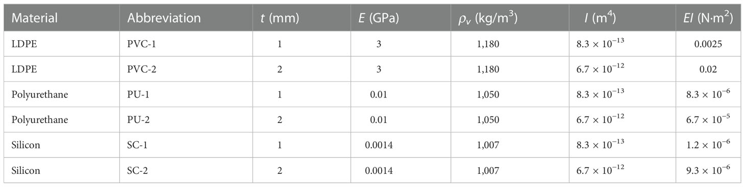
Table 1 Physical parameters of the model vegetation.

A submersible pump controlled the inlet flow, which was measured using an electromagnetic flowmeter. A steel rectification grid was installed at the tank inlet to provide a smooth and uniform inlet flow. Water depth was measured by four water gauges arranged along the course. For all the experimental test conditions, the flow in the experimental layer reached a quasi-steady and uniform status. The test was configured with six planted forms (see Table 1), each with five inlet bulk flow velocities of 0.06, 0.084, 0.11, 0.14, and 0.17 m/s. The corresponding flow was 5.5, 8.4, 11.3, 14.1, and 17.0 L/s, respectively. A small uncertainty of 4% in the electromagnetic flowmeter reading was caused by the small fluctuation of pump flow. For all the experimental conditions, a constant water depth of 0.25 m was chosen to compare the effects of the different flexible vegetation on the hydrodynamics and turbulence characteristics along the vertical direction (Li et al., 2018). The Ca of vegetation canopy under natural environmental settings ranges from 0.001 to 1,000; in this paper, it ranged from 0.002 to 73.009 for all experimental conditions. As seen in Table 2, the buoyancy parameter, B, of the model vegetation under all working conditions was less than 1 because the difference between the densities of the three materials used was much smaller than the difference between their elastic moduli. It can be assumed that the vegetation stiffness dominated the restorative force relative to the buoyancy experienced by the vegetation in the experiments (Zhang et al., 2020b). Therefore, the effect of the buoyancy of the vegetation on the deflected height of the vegetation, h_e, is not considered in this study.

TABLE 2

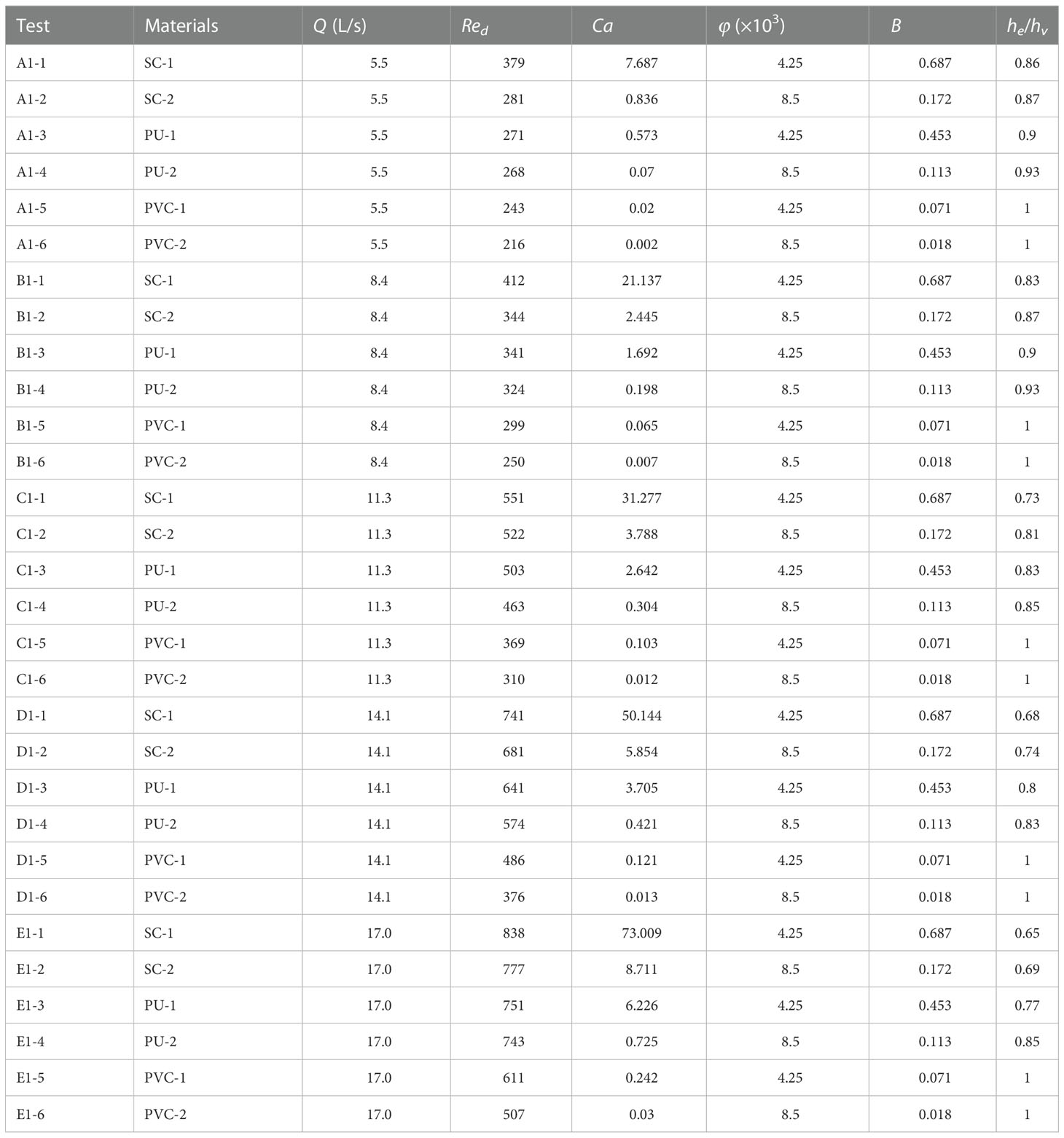
Table 2 Vegetation and flow parameters for each test.

Two-dimensional particle image velocimetry (2D-PIV) was used to measure the flow field in the longitudinal profile (x–z plane), and a sheet laser emitter was mounted below the bottom wall of the unidirectional flume with a maximum laser power of 10 W. The sheet laser illuminated the flow vertically from the bottom, parallel to the side wall of the unidirectional flume, with a thickness of 1.5 mm. A high-speed camera (MindVision, MV-XG4701C/M/T) was mounted on the side of the unidirectional flume and aligned vertically with the sheet laser. The camera had a maximum effective pixel count of 47 million and a maximum resolution of 8,240 × 5,628. The exposure time was set to 120 μs, considering the image contrast and particle trailing. Due to the computer hardware configuration, the camera’s low frame rate at the highest pixel, and the transmission speed, the camera could operate only in the low pixel-high frame rate mode; therefore, after testing and comparison, 6,600 snapshots were taken for each condition with an image size of 1,280 × 960 pixels and a sampling frequency of 333 Hz. After testing and selection, polyamide resin particles (PSP) with a diameter of 10 μm, a density of ~1.03 g/cm³, and a refractive index of 1.2 were used as tracers. Referring to a study by Okamoto et al. (2016), we positioned the irradiating sheet laser on the side of the model canopies as detailed in Figure 1. The FOV was located at the end of the vegetation patch to ensure that the flow was fully developed (Lei and Nepf, 2021). PIVlab was used to acquire the snapshots for processing (Thielicke and Stamhuis, 2014). After removing the background, the snapshots were preprocessed using a contrast-constrained adaptive histogram equalization technique. The intensity capping technique was used to minimize the error. The PIV snapshot pairs were analyzed using the FFT-based multi-pass algorithm with multiple grid iteration methods using an interrogation window size of 40 × 40, a minimum first-level window size of 20 × 20, and a 50% spatial overlap in both directions. The Gauss 2 × 3-point method was used for the sub-pixel estimator, providing a vector grid spacing of Δx = 2.13 mm and Δz = 2.13 mm. The initial flow vector field was subsequently post-processed to remove and replace bad vectors by using standard deviations and median filters with predefined thresholds. The flow field timing file consisting of all snapshots was saved in.dat format, and the turbulence statistical variables were computed by a post-processing program written in Python. We fixed the camera outside the glass window of the flume with the lens facing perpendicular to the center of the slice laser. During each sampling period, the motion of the model vegetation under the sheet laser irradiation was recorded by the camera. The camera sampling time was 2 min for each sampling. Time-averaged deflected height of the model vegetation canopy was obtained by analyzing the motion sequence with computer vision software.

FIGURE 1

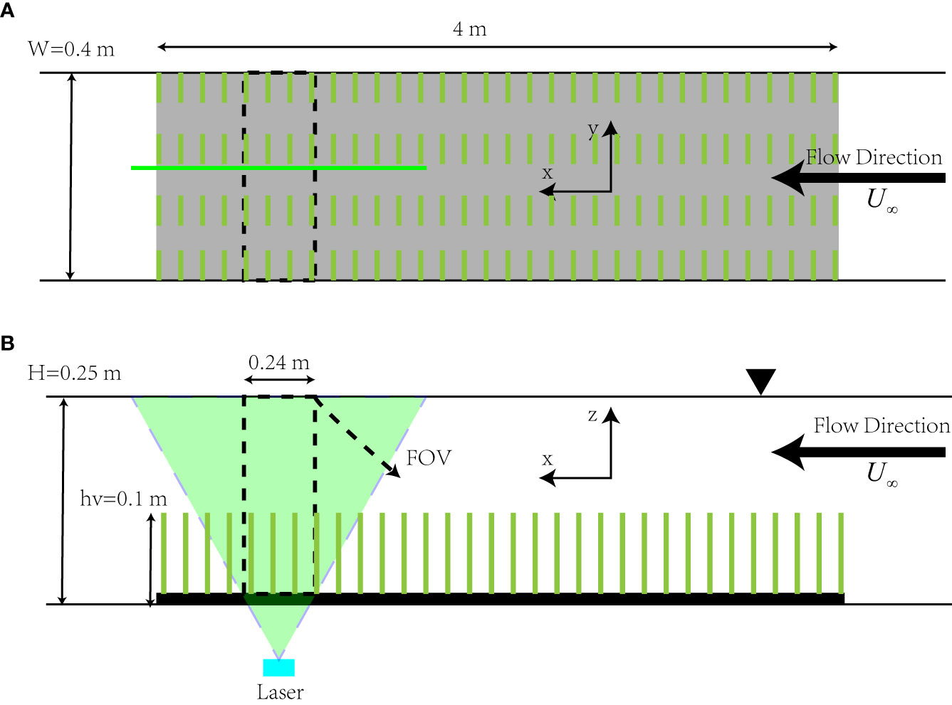
Figure 1 Views of the experimental section (not to scale), where the black dashed line in the figure is the PIV acquisition area (FOV): (A) top view; (B) side view.

4 Results

4.1 Velocity

Figure 2 shows the distribution of dimensionless time-average streamwise velocity, $\overline{u}/U_{\infty },$ and dimensionless double-averaged streamwise velocities, $\langle \overline{u}\rangle /U_{\infty }$, under different tests. The vertical coordinate, z, was dimensionless with respect to the undeflected height of vegetation, h_v, where z/h_v = 0 corresponds to the bed; z/h_v = 1 corresponds to the undeflected height of the vegetation position (green dashed line), and z/h_v = 2.5 corresponds to the free surface. As compared with the rigid vegetation, reconfiguration of the flexible vegetation stems significantly reduces the turbulence around the canopy top, leading to a flatter mean shear. It also reduces the local velocity gradient. At the same time, the “Monami” phenomenon of flexible vegetation greatly promotes the efficiency of momentum transmission from outside the canopy to the inside of it. Therefore, under the same flow rate, the canopy-averaged velocity for flexible vegetation is higher than that for rigid vegetation. As can be seen in Figures 2C, D, the $\langle \overline{u}\rangle /U_{\infty }$ trend for both rigid and flexible submerged vegetation showed an inverted “S” shape distribution along the vertical direction. From the bed, along the vertical direction, $\langle \overline{u}\rangle /U_{\infty }$ gradually increased; the velocity variation near the bed was small, and the velocity gradient, d($\langle \overline{u}\rangle /U_{\infty }$)/dz, near the top of the vegetation canopy was larger. There was an obvious shear point around the vegetation canopy top as $\langle \overline{u}\rangle /U_{\infty }$ reached its maximum value at a certain distance below the free surface and then maintained this value until the free surface. For the same vegetation volume, as the vegetation thickness t increased, its volume fraction, φ, increased accordingly. The submerged vegetation had a greater ability to block the flow; therefore, $\langle \overline{u}\rangle /U_{\infty }$ within the vegetation canopy decreased and increased outside of it, while d($\langle \overline{u}\rangle /U_{\infty }$)/dz near the top of the vegetation canopy also increased. When comparing PVC-1 with PU-2 (tests A1-5 with A1-4 or tests E1-5 with E1-4), the model vegetation corresponding to PU-2 presented a higher vegetation volume fraction, φ, due to lower modulus of elasticity, but the model vegetation underwent reconfiguration under the flow due to which its deflected height ratio, h_e/h_v, decreased, thus making PU-2 less capable of blocking flow than PVC-1. A similar phenomenon was observed upon a comparison of PU-1 with SC-2. As the Reynolds number, Re_d, of the vegetation canopy increased, the vertical distribution of the dimensionless velocity, $\langle \overline{u}\rangle /U_{\infty }$, did not change significantly for rigid submerged vegetation. Contrarily, the distribution of $\langle \overline{u}\rangle /U_{\infty }$ along the vertical direction presented a decrease in h_e/h_vfor flexible submerged vegetation. The opposing trends of $\langle \overline{u}\rangle /U_{\infty }$ and d($\langle \overline{u}\rangle /U_{\infty }$)/dz with h_e/h_v above and within the vegetation canopy were particularly evident in modeled submerged vegetation with very low modulus of elasticity, such as SC-1. We found that in the test E1-1, the h_e/h_v was reduced to 0.63, while the “Monami” phenomenon occurred with a large oscillation, which greatly facilitated the transfer of first- and second-order momentum from the area outside the vegetation canopy to the area inside the vegetation canopy by bidirectional fluid–structure interaction. This also led to the distribution of $\langle \overline{u}\rangle /U_{\infty }$ along the vertical direction being different from the other test conditions, but it was similar to the distribution for test V3-9 in a study by Li et al. (2018). Overall, when the vegetation volume fraction was the same, $\langle \overline{u}\rangle /U_{\infty }$ and d($\langle \overline{u}\rangle /U_{\infty }$)/dz increased as h_e/h_v decreased within the vegetation canopy; they decreased as h_e/h_v decreased outside the vegetation canopy. These patterns suggest that the reconfiguration of flexible submerged vegetation affects the efficiency of momentum transfer along the vertical direction and also reduces the ability of the vegetation to block water flow.

FIGURE 2

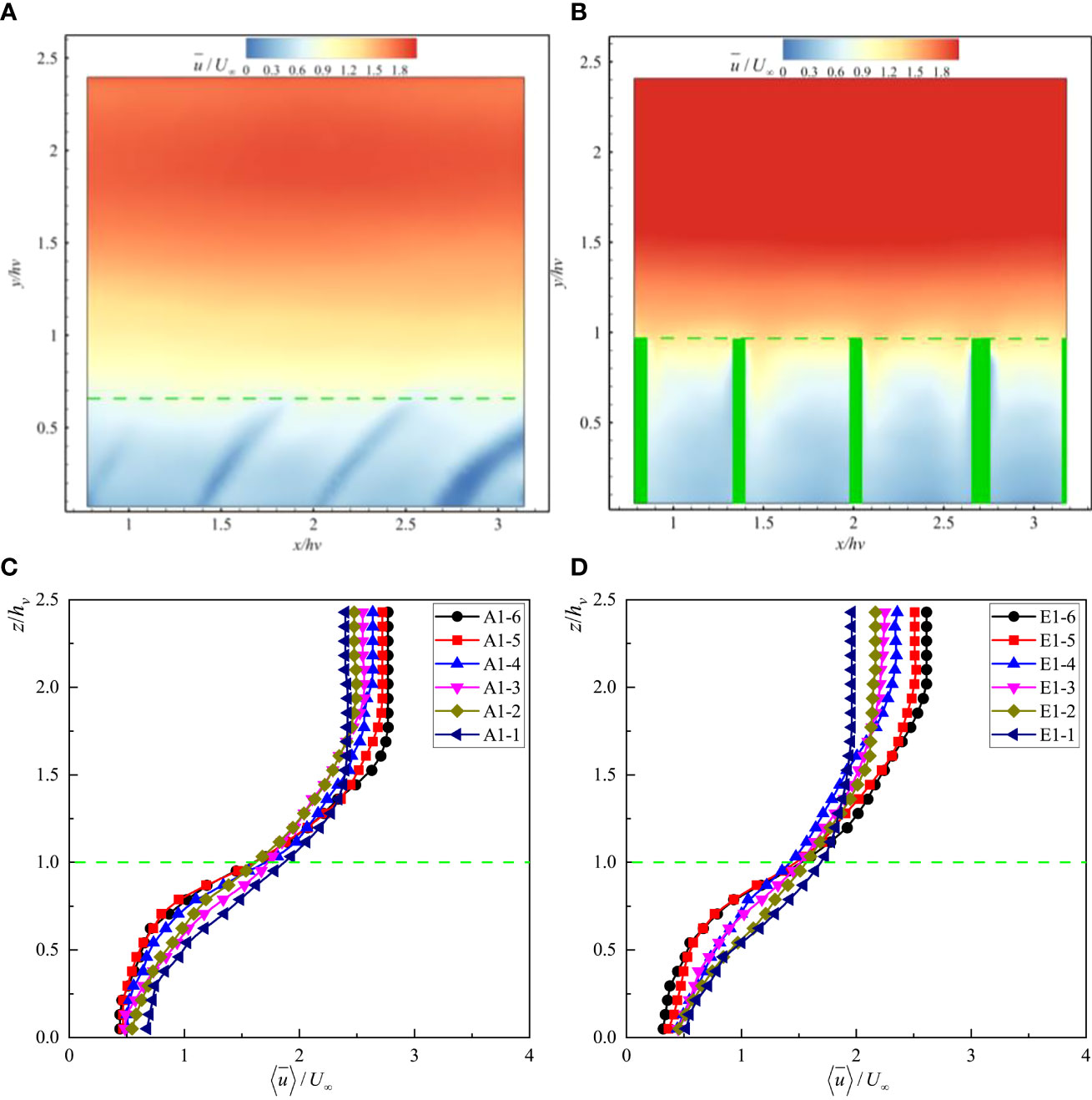
Figure 2 Distribution of the dimensionless time-averaged streamwise velocity $\langle \overline{u}\rangle /U_{\infty }$ under (A) E1-1 and (B) E1-5 and the distribution of the dimensionless double averaged streamwise velocity $\langle \overline{u}\rangle /U_{\infty }$ under (C) Test A and (D) Test E.

4.2 Reynolds stress

Figure 3 shows the distribution of dimensionless time-average Reynolds stresses $-\overline{u^{\prime }{w}^{\prime }}/U_{\infty }^2$ and the dimensionless space-time averaged Reynolds stresses $-\langle \overline{u^{\prime }{w}^{\prime }\rangle }/U_{\infty }^2$ under different tests. It can be seen from the figure that the reconfiguration (bending and streamlining) of flexible vegetation is more conducive to the transfer of turbulent energy from the outside of the canopy to its inside for rigid vegetation, which significantly reduces the peak $-\overline{u^{\prime }{w}^{\prime }}/U_{\infty }^2$ near the canopy top. Therefore, the coherent structure of turbulence can be more readily extended to the deeper part of the canopy in the flexible vegetation compared to the rigid vegetation (Li et al., 2018). It can be seen from Figures 3C, D that the Reynolds stress, $-\langle \overline{u^{\prime }{w}^{\prime }}\rangle /U_{\infty }^2$, gradually increased from the free surface vertically, reaching a maximum value near the top of the vegetation canopy. It then decreased rapidly along the vertical direction and remained constant near the bed. A similar pattern was presented by $\langle \overline{u}\rangle /U_{\infty }$, for the same vegetation material, whereby with an increase in vegetation thickness, t, the vegetation fraction, φ, increased. The blockage effect of the vegetation canopy was also more substantial; therefore, $-\langle \overline{u^{\prime }{w}^{\prime }\rangle }/U_{\infty }^2$ and its maximum value also increased along the vertical direction. When the vegetation fraction, φ, was the same, with a gradual decrease in h_e/h_v, the peak value of Reynolds stress near the top of the vegetation canopy gradually decreased. The position, where the Reynolds stress reached a minimum outside the vegetation canopy, was closer to the top of the vegetation canopy, while the position where it reached the minimum value within the vegetation canopy was closer to the bed; i.e., the vertical distribution of $-\langle \overline{u^{\prime }{w}^{\prime }\rangle }/U_{\infty }^2$ was closer to that without submerged vegetation (Dijkstra and Uittenbogaard, 2010). The double-averaged Reynolds stress distribution within the vegetation canopy of the flexible submerged vegetation was more uniform than that of the rigid submerged vegetation, indicating that the flexible submerged vegetation transfers a part of the turbulent energy from the outside of the vegetation canopy to its inside through reconfiguration.

FIGURE 3

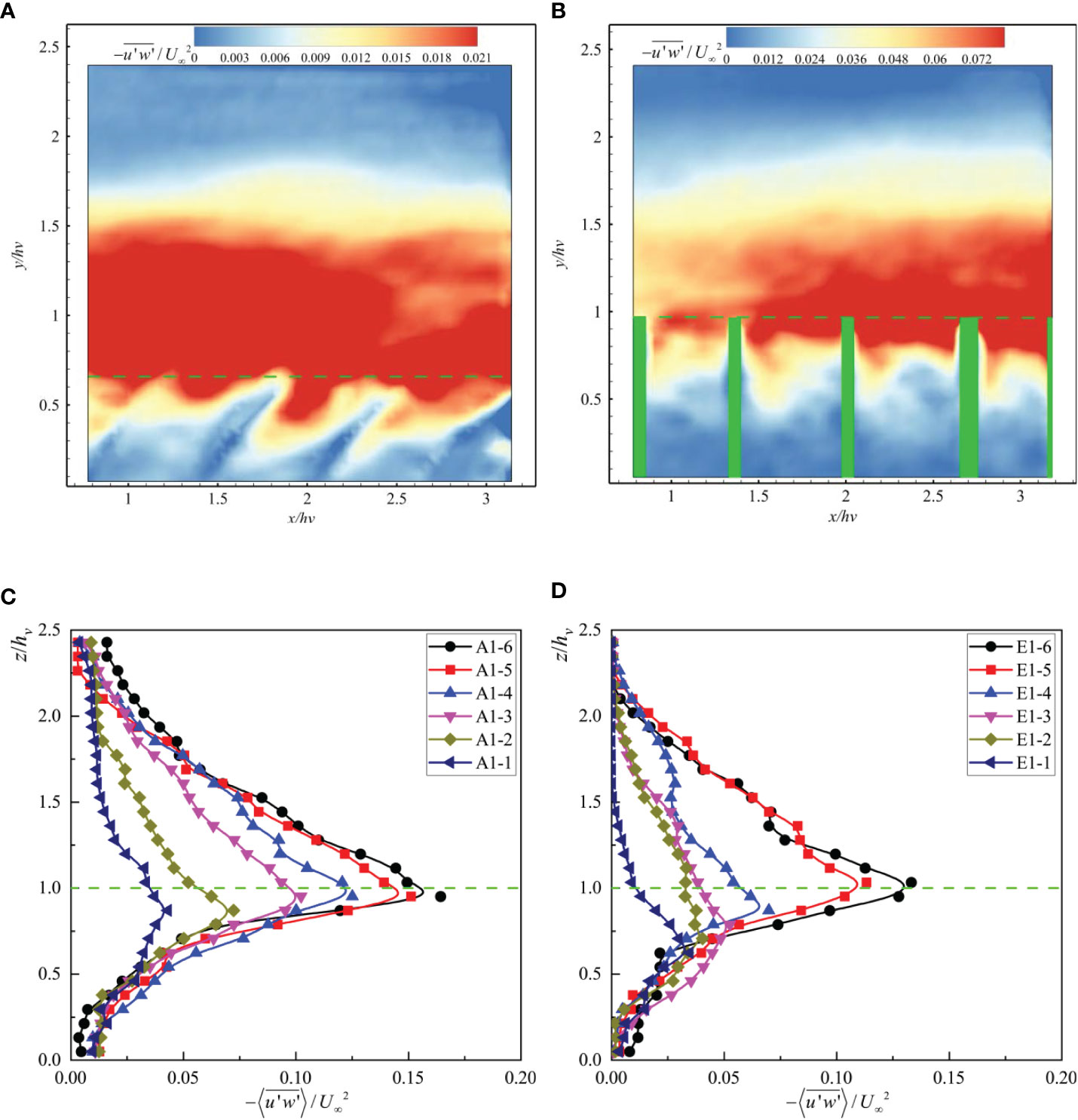
Figure 3 Distribution of the dimensionless time-averaged Reynolds stress $-\langle \overline{u^{\prime }{w}^{\prime }\rangle }/U_{\infty }^2$ under (A) E1-1 and (B) E1-5 and the distribution of the dimensionless double-averaged Reynolds stress $-\langle \overline{u^{\prime }{w}^{\prime }\rangle }/U_{\infty }^2$ under (C) Test A and (D) Test E.

As can be seen in Figure 3, the Reynolds stress decreased rapidly in the vertical direction after entering the vegetation canopy due to the blockage effect of vegetation stems hindering the efficiency of momentum transfer from the outside to the inside of the vegetation canopy. Many scholars have also observed this phenomenon in experiments. Nepf and Vivoni (2000) equated the measurement of the exchange momentum region inside and outside the vegetation canopy with the distance that the Reynolds stress, $-\langle \overline{u\text{'}w\text{'}\rangle }$, penetrates through the vegetation canopy; they proposed the penetration depth of the Reynolds stress, δ_e, which is defined as the distance required to reduce the Reynolds stress from the maximum near the top of the vegetation canopy to a value that is 10% of the maximum. The relationships between the dimensionless penetration depth, δ_e/h_e, and the Reynolds number of the vegetation canopy, Re_d, under different test conditions are given in Figure 4, where the uncertainty caused by this spatial change was 6%. For the same vegetation material, the larger the vegetation fraction, the greater the vegetation resistance within the canopy. It was also more difficult for the Reynolds stress caused by KH instability vortex and shear near the top of the vegetation canopy to penetrate the whole vegetation canopy, and thus, the dimensionless penetration depth, δ_e/h_e, was smaller. Due to the reconfiguration, swaying, and the “Monami” phenomenon of flexible submerged vegetation, the bulk resistance within the vegetation canopy was smaller, making it easier for the shear vortex to penetrate the whole vegetation canopy (Okamoto and Nezu, 2010). In contrast, rigid submerged vegetation is expected to be more effective in destroying the coherent eddy structure near the top of the vegetation canopy than the flexible submerged vegetation, thus reducing the penetration capacity of Reynolds stress. Overall, the dimensionless penetration depth, δ_e/h_e, increases with increasing Re_d, while δ_e/h_e increases with increasing Ca for the same Re_d.

FIGURE 4

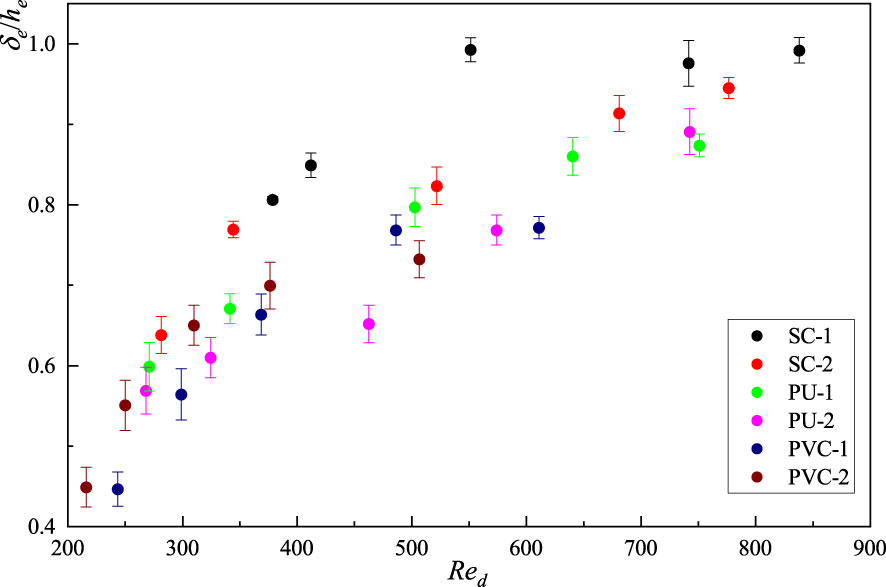
Figure 4 The relationship between dimensionless penetration depth, δ_e/h_e, and vegetation canopy Reynolds number, Re_d, under different test conditions.

4.3 Drag coefficient

Figures 5A, B show the vertical distribution characteristics of the local drag coefficient, C_dl, calculated by Eq. 1 under different test conditions. At the position near the bed, due to the influence of wake and resistance of vegetation stems, the vertical flow velocity was almost constant, and the Reynolds stress gradient in this area was also small. Therefore, the change in C_dl in this area was relatively small, which is similar to the local drag coefficient distribution of emergent vegetation (Nepf and Vivoni, 2000). In the area near the top of the vegetation canopy, C_dl decreased rapidly with an increase in z/h_v. Similar phenomena were observed by Li et al. (2018) and Tang et al. (2014), especially when the relative submergence was large. This phenomenon may be caused by the relaxation of the shape resistance caused by the bleeding behavior of the flow near the top of the model vegetation leaves (Ghisalberti and Nepf, 2006). With the same vegetation material, the local drag coefficient, C_dl, along the vertical direction increased as φ increased. As the modulus of elasticity of the vegetation decreased, the vegetation began to undergo reconfiguration, h_e/h_v decreased, and the maximum value of C_dl along the vertical direction decreased. For rigid submerged vegetation, the position, where the maximum value of C_dl appeared consistently, was located near z/h_e = 0.8. For flexible vegetation with a small elastic modulus, such as SC-1, when the bulk flow was large and the hydrodynamic force on the vegetation was far greater than the restorative force caused by the stiffness, the vegetation underwent strong reconfiguration; in such a case, the position, where the maximum value of C_dl appeared, decreased to h_e/h_v= 0.54. Under all working conditions, the position of the maximum value of C_dl along the vertical direction was between 0.7h_e and 0.8h_e, which is consistent with the studies of Tang et al. (2014) and Ghisalberti and Nepf (2004b). For the same z/h_e position, with a gradual decrease in h_e/h_v, the local drag coefficient, C_dl, also gradually decreased, indicating that the reconfiguration of vegetation reduced the blockage of vegetation within the canopy.

FIGURE 5

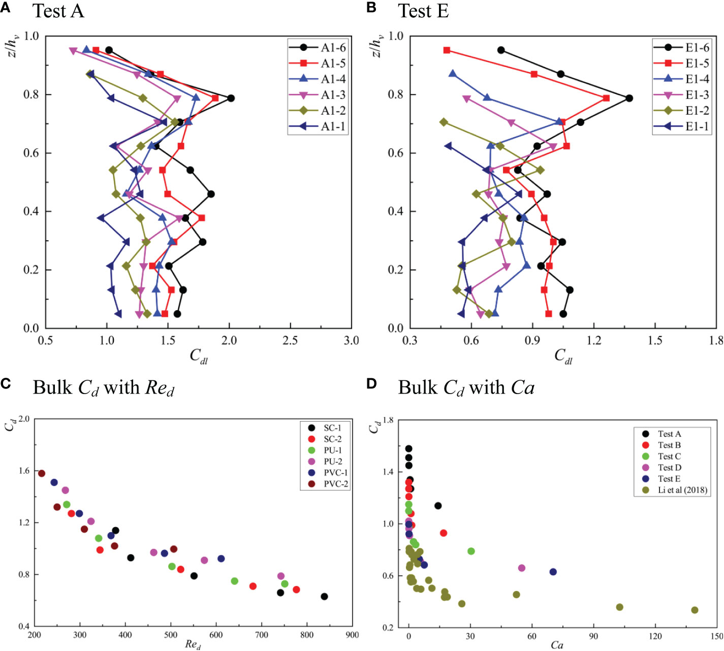
Figure 5 The vertical distribution of local drag coefficient, C_dl under (A) Test A and (B) Test E and the relationship between C_d and Re_d (C) and between C_d and Ca (D).

The bulk drag coefficient, C_d, can be obtained by averaging the bulk drag coefficient, C_dl, within the deflected height, h_e, of the vegetation. Figures 5C, D, respectively, show the relationship between the bulk drag coefficient, C_d, Re_d, and Ca under different test conditions. With an increase in Re_d, C_d gradually decreased. When Re_d increased to 700, C_d tended to gradually stabilize. At the same time, with the same Re_d, C_d decreased with an increase in Ca. It can also be seen from the figure that there was a regular exponential relationship between the bulk drag coefficient and the Cauchy number of the vegetation canopy. In addition, C_d was positively correlated with φ, which is consistent with the report of Li et al. (2018), indicating that it is feasible to predict the bulk drag coefficient using Ca. Luhar and Nepf (2011) proposed a scaling law to correlate the effective length, drag force, and Ca^-1/3 based on the force balance between resistance and the restorative force caused by stem stiffness. Based on the above description and other relevant research (Sonnenwald et al., 2018), we believe that the relationship between the bulk drag coefficient, C_d, the Reynolds number of the canopy, Re_d, the Cauchy number of the canopy, Ca, and the vegetation fraction, φ, can be described by the following formula:

$\begin{array}{ll}{C}_d=\frac{a1}{R{e}_d}+a2C{a}^{-1/3}+a3\phi +a4& (15)\end{array}$

Among these, a1–a4 are the coefficients to be determined. The general global optimization method and quasi-Newton method were used to conduct nonlinear regression analyses on the relationship between C_d, Re_d, Ca, and φ, and finally, the fitting Eq. 16 was obtained:

$\begin{array}{ll}{C}_d=\frac{238}{R{e}_d}+0.01C{a}^{-1/3}+6.2\phi +0.38& (16)\end{array}$

From Eq. 16, it can be seen that C_d was negatively correlated to Re_d and Ca, but positively correlated to φ, which is consistent with a previous study (Liu et al., 2020). In addition, Figure 6 shows a comparison between the predicted value of the bulk drag coefficient, C_d, and the measured value. It can be seen that the data were distributed on both sides of the perfect agreement line, and the determination coefficient, R², was 0.858. Therefore, in the turbulent kinetic energy model (TKE model) within the vegetation canopy, the determination of the bulk drag coefficient adopted Eq. 16.

FIGURE 6

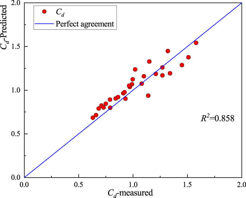
Figure 6 A comparison of the predicted and measured values of bulk drag coefficient, C_d, under different test conditions.

4.4 Turbulent kinetic energy

The turbulent kinetic energy characterizes the degree of local turbulence. Figures 7A, B shows the spatial distribution of $k/U_{\infty }^2$ for two test conditions and Figures 7C, D presents the spatially averaged turbulent kinetic energy, $k/U_{\infty }^2$, for the different test conditions. As can be seen from the figure, the distribution of $k/U_{\infty }^2$ is similar to that of $-\overline{u^{\prime }{w}^{\prime }}/U_{\infty }^2$. The reconfiguration of flexible vegetation enhanced the efficiency of turbulent energy transport along the vertical direction, leading to lowered $k/U_{\infty }^2$ near the top of the canopy as compared to the rigid vegetation. The maximum value of $\mathrm{\langle k\rangle }/U_{\infty }^2$ along the vertical direction occurred near the top of the vegetation canopy and gradually decreased along the free surface and the bed. The average vertical gradient of turbulent kinetic energy, d $\mathrm{\langle k\rangle }/U_{\infty }^2$/dz, in the area within the vegetation canopy was greater than the average vertical gradient in the area outside the vegetation canopy. For the same vegetation material, the spatially averaged turbulent kinetic energy, $\mathrm{\langle k\rangle }/U_{\infty }^2$, along the vertical direction increased with an increase in φ. Overall, when the vegetation fraction, φ, was the same, the turbulent kinetic energy along the water depth gradually decreased with a gradual decrease in h_e/h_v. At the same time, with a decrease in h_e/h_v, the location of the maximum $\mathrm{\langle k\rangle }/U_{\infty }^2$ also decreased. In general, the reconfiguration of vegetation reduced the turbulence under unidirectional flow.

FIGURE 7

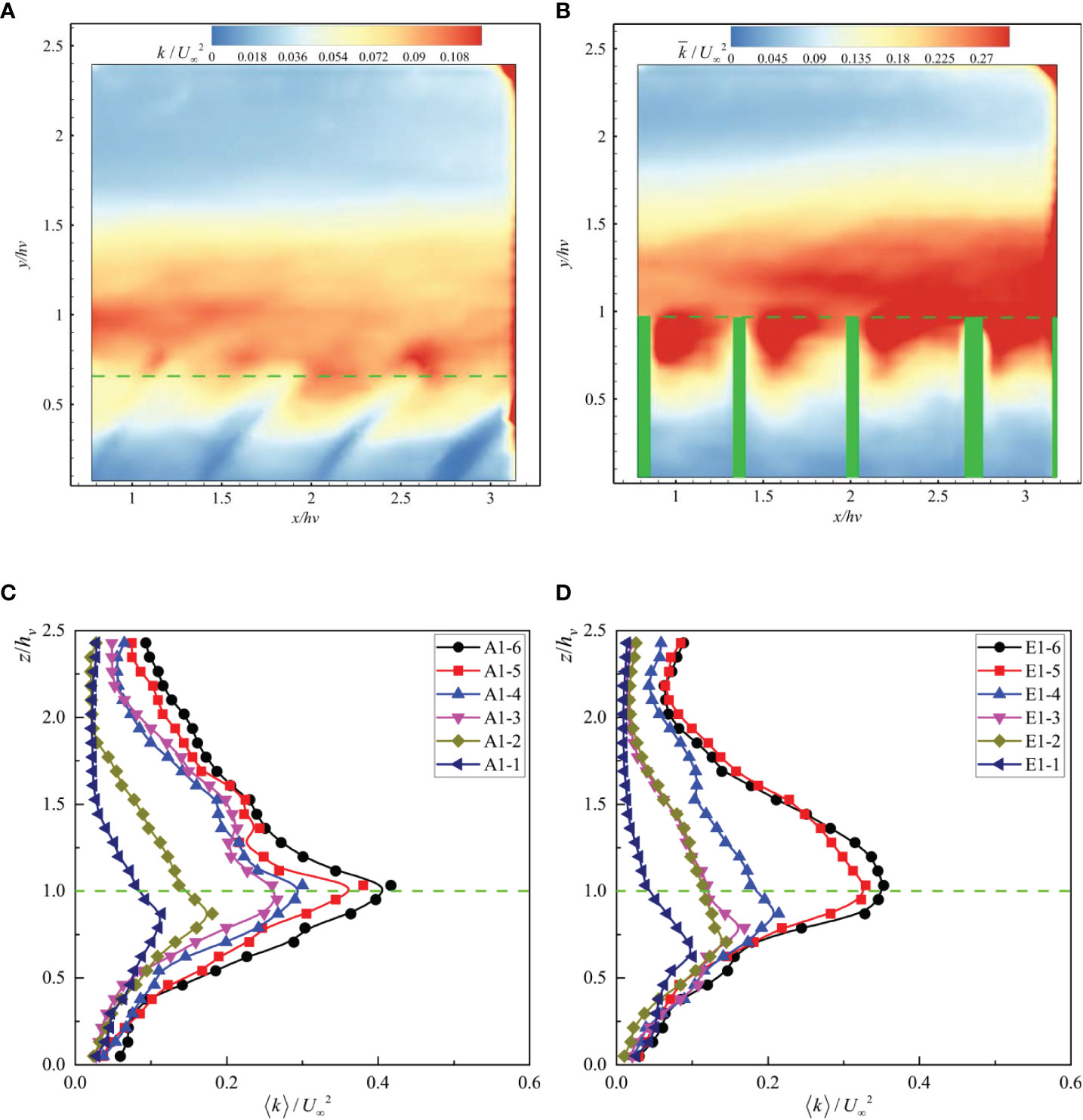
Figure 7 The distribution of dimensionless time-averaged turbulent kinetic energy $k/U_{\infty }^2$ under (A) E1-1 and (B) E1-5 and the dimensionless double-averaged turbulent kinetic energy, $\mathrm{\langle k\rangle }/U_{\infty }^2,$ under (C) Test A and (D) Test E.

The canopy-averaged turbulent kinetic energy, k_c, can be obtained by averaging the spatially averaged turbulent kinetic energy, 〈k〉 , within the deflected height, h_e, of the vegetation. Figure 8 shows the relationship between the canopy-averaged turbulent kinetic energy, $k_c/U_{\infty }^2$, with the Cauchy number of the vegetation canopy, Ca, under different test conditions. Due to the reconfiguration of the flexible submerged vegetation, h_e/h_v decreased, making the blocking effect of the flexible submerged vegetation lower than that of the rigid submerged vegetation. Therefore, $k_c/U_{\infty }^2$ decreased with an increase in the canopy Cauchy number, Ca.

FIGURE 8

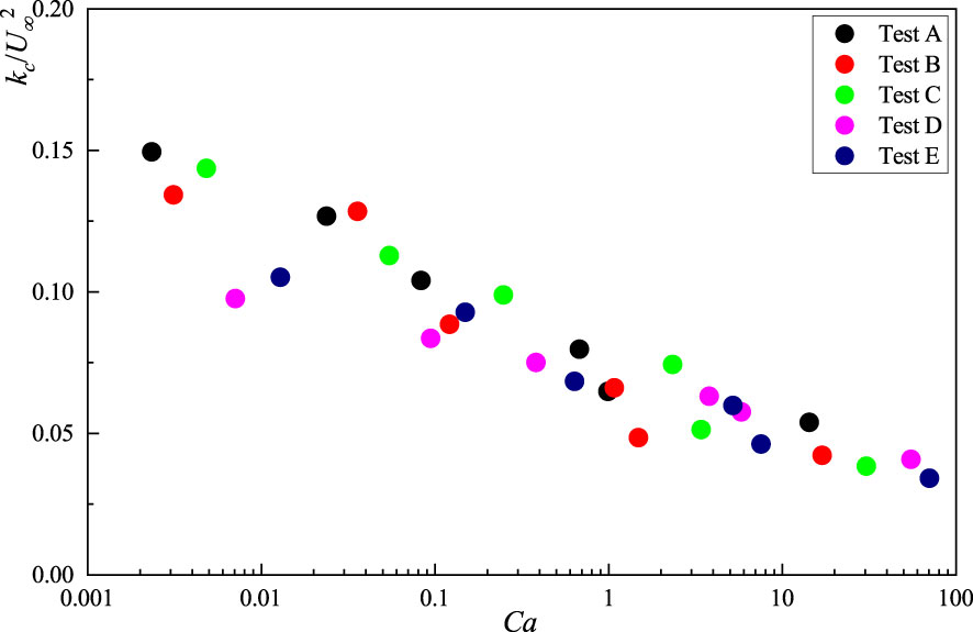
Figure 8 The relationship between canopy-averaged turbulent kinetic energy, $k_c/U_{\infty }^2$, and the Cauchy number of the vegetation canopy, Ca.

5 Discussion

5.1 The characteristics of the shear layer

To study the influence of vegetation flexibility on the structure of vegetation around the canopy top (Bailey and Stoll, 2016), we calculated the time-averaged vorticity under four conditions; the results of these test conditions are compiled in Figure 9. It can be seen from the figure that there is a peak value of $\overline{{\omega }_y}$ near the canopy top, and the overall distribution is similar to $k/U_{\infty }^2$ and $-\overline{u^{\prime }{w}^{\prime }}/U_{\infty }^2$. In the case of rigid vegetation, the maximum $\overline{{\omega }_y}$ near the canopy top and the area affected by high vortices were larger than those recorded for flexible vegetation, indicating that the average shear near the top of rigid vegetation canopy is stronger (Nezu and Sanjou, 2008). This phenomenon could be attributed to the fact that with an increase in Re_d, the stems of flexible vegetation begin to wave and h_e/h_v decreases accordingly, leading to less blockage compared to rigid vegetation. Therefore, the intensity of the coherent structure caused by Kelvin–Helmholtz instability and the range of its influence are also weaker than those for rigid vegetation (Li et al., 2018). This phenomenon can also be explained by the relationship between the dimensionless velocity difference, the dimensionless mixing layer thickness, and the Cauchy number of the canopy.

FIGURE 9

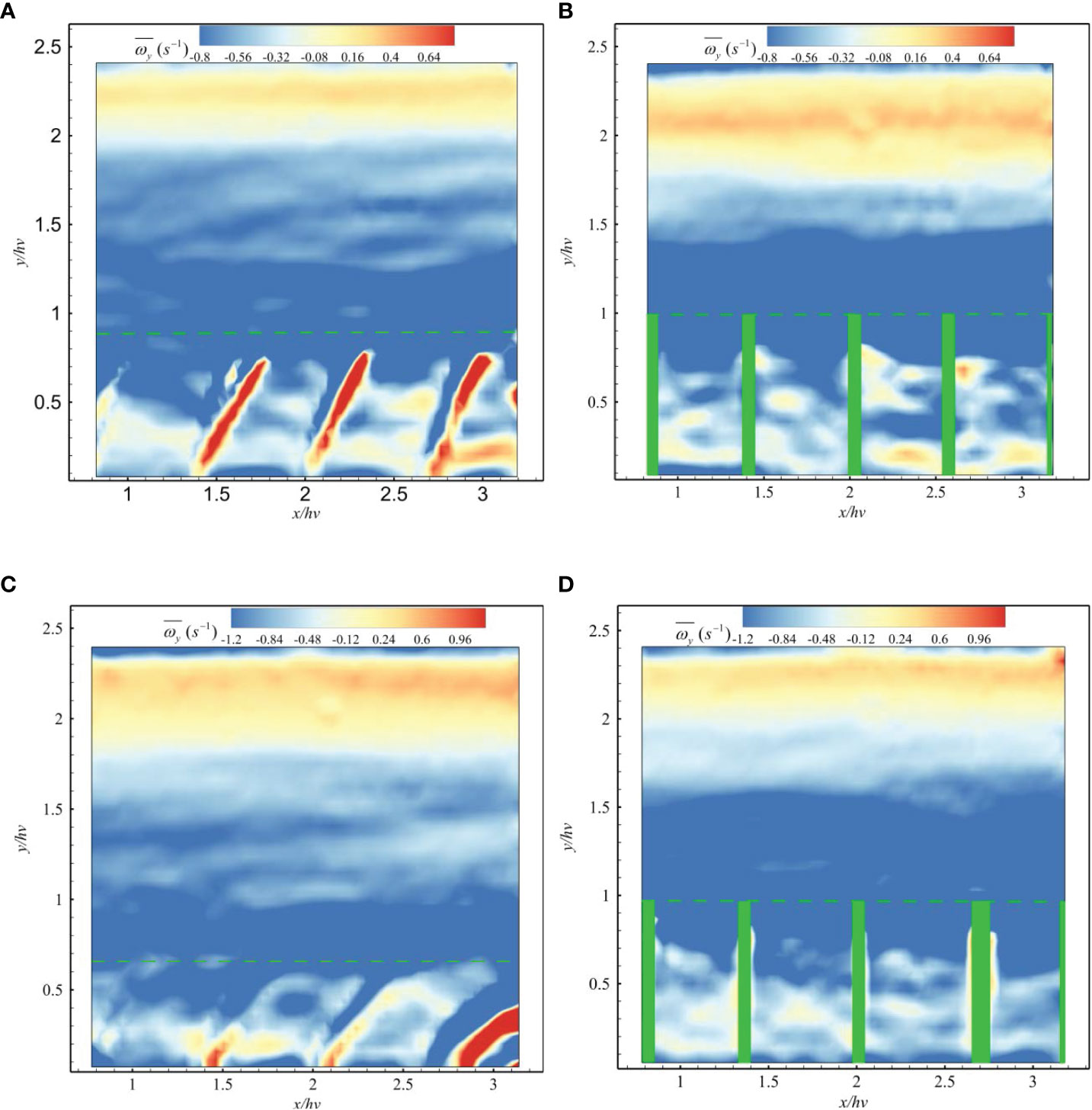
Figure 9 The distribution of the time-averaged vorticity $\overline{{\omega }_y}$ under (A) A1-1, (B) A1-5, (C) E1-1, and (D) E1-5.

Figure 10A presents the relationship between the dimensionless velocity difference, Δu/U_∞ , between the interior and exterior of the vegetation canopy, as well as the Ca for different test conditions; here, the x-axis is in log scale because the uncertainty caused by spatial change is 3%. For the same vegetation material and U_∞, Δu/U_∞ increased with φ and gradually decreased with Ca. As Re_d increased, Δu/U_∞ changed less for the rigid submerged vegetation, while it decreased with an increase in Re_d for the flexible submerged vegetation. This phenomenon is attributed to the increase in Re_d causing a gradual decrease in the h_e/h_v of the flexible submerged vegetation; it is also associated with the profile of $\overline{u}/U_{\infty }$ along the vertical direction tending to be more similar to the distribution seen with the classical unidirectional flow. Figure 10B depicts the relationship between the dimensionless mixed layer thickness, T_ml/H, and the Reynolds number, Re_d, of the vegetation canopy. Here, T_ml/H is defined as the distance between z_0.9 and z_0.1, where z_0.1 corresponds to the height of U₁+0.1ΔU and z_0.9 corresponds to the height of U₁+0.9ΔU; the definitions of U₁ and ΔU can be found in Ghisalberti and Nepf (2004a). The uncertainty caused by this spatial change was 5%. T_ml/H increased with increasing Re_d in both rigid and flexible submerged vegetation within the error range. The increase in T_ml/H with increasing Re_d was lower for flexible submerged vegetation than for rigid submerged vegetation. For the former, h_e/h_v gradually decreased with increasing Re_d, resulting in a smaller increase in the strength and extent of the influence of coherent eddies near the top of the vegetation canopy. Overall, the dimensionless mixed layer thickness, T_ml/H, was positively correlated with Re_d and negatively correlated with Ca.

FIGURE 10

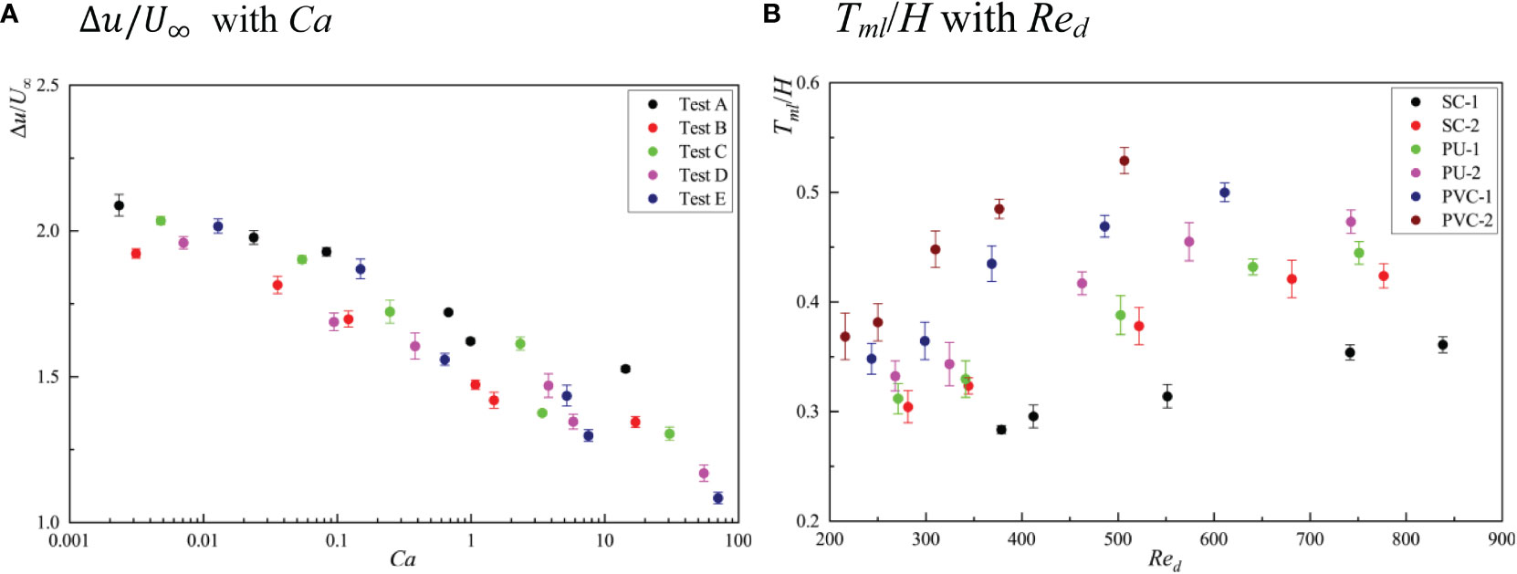
Figure 10 Relationships of Δu/U_∞ and T_ml/H with Ca (A) and Re_d (B).

5.2 Shear and wake production terms

The elevated turbulent kinetic energy within the canopies under unidirectional flow can be attributed to two aspects. Firstly, turbulence can be generated in the wake area behind the vegetation stems. Secondly, the shear eddies caused by Kelvin–Helmholtz instability can occur near the top of the vegetation canopy, thus causing an increase in turbulent kinetic energy. Figure 11 shows the distribution of the shear production term, P_s, the wake production term, P_w, and the total production terms of turbulent kinetic energy, P_t, along the vertical direction under different test conditions; P_s was estimated using Eq. 2 and P_w was estimated by Eq. 5. As the wake production is only generated behind the vegetation stems, the calculation range is within the vegetation canopy, and P_t is the sum of the first two terms. As can be seen from the figure, P_s reached a maximum value at the top of the vegetation canopy due to the largest velocity gradient in this region, which is consistent with studies by Devi and Kumar (2016) and Termini (2019). P_s decreased rapidly as it entered the vegetation canopy and tended to become zero near the bed due to the blocking effect of the vegetation canopy. P_w reached a maximum value near the top of the vegetation canopy, while, upon entering it, local P_w was always greater than P_s. For the same flow rate, P_s, P_w, and P_t were greater for rigid submerged vegetation than for flexible submerged vegetation along the vertical direction, suggesting that a reduction in h_e/h_v significantly reduces the degree of turbulence within the vegetation canopy.

FIGURE 11

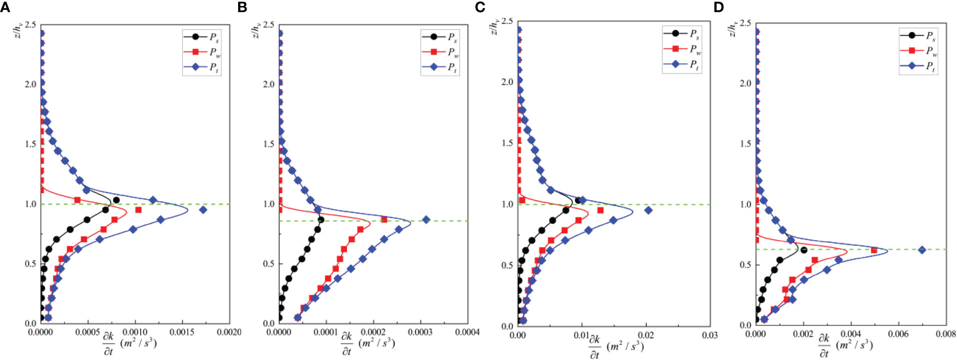
Figure 11 Vertical distributions of the shear production term, P_s, the wake production term, P_w, and the total production term, P_t, of turbulent kinetic energy under (A) A1-5, (B) A1-1, (C) E1-5, and (D) E1-1.

To compare the average contribution of the shear production term, P_s, to the turbulent kinetic energy within the vegetation canopy, we defined R_s/t as follows:

$\begin{array}{ll}{R}_{s/t}=\frac{100}{h_e}\underset{0}{\overset{h_e}{\int }}\left(P_s/P_t\right)dz& (17)\end{array}$

A larger value of R_s/t indicates a larger ratio of the shear production term, P_s, to the total production term, P_t. Figure 12 shows the relationships between the vegetation canopy-averaged contribution of shear production term, R_s/t, and Ca under different test conditions. Figure 10 depicts that with an increase in Ca, the R_s/t gradually decreased.

FIGURE 12

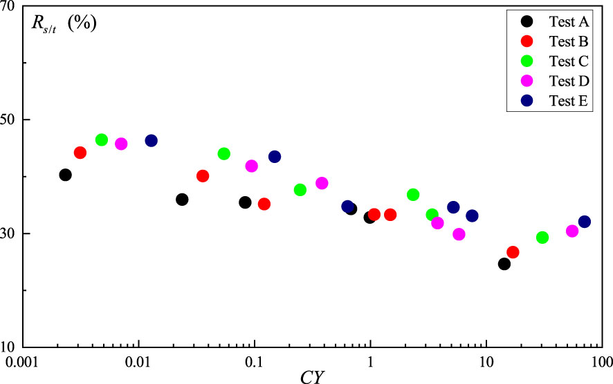
Figure 12 The relationship between R_s/t and the Cauchy number Ca.

The shear production of turbulent kinetic energy is mainly controlled by the large-scale coherent structure near the canopy top induced by the Kelvin–Helmholtz instability (Ghisalberti and Nepf, 2001). As compared to rigid vegetation, flexible vegetation reduces P_s through two mechanisms. First, h_e/h_v gradually decreases with an increase in Ca, weakening the blockage effect and reducing the relative coherent structure strength near the canopy top (see Section 5.1). Second, the “Monami” phenomenon of flexible vegetation enhances the vertical transportation of turbulent energy, which may transport more turbulent energy to the interior of the canopy than the rigid vegetation, thus reducing P_s. The results from a study by Zhang et al. (2020a) demonstrated that the mean P_s within the vegetation canopy increased with a·h_e, while P_w decreased with a·h_e. In addition, the value of R_s/T gradually increases and converges to 50% as a·h_e increases. Corresponding to the present experiment, for constant flow rate, as Ca increases, h_e gradually decreases, corresponding to a·h_e, which also gradually decreases, so that R_s/T decreases with increasing Ca. In addition, under all test conditions investigated here, R_s/t ranged between 24% and 48%, indicating that the importance of shear production should not be ignored.

5.3 Prediction of turbulent kinetic energy within the vegetation canopy

To apply the TKE model, we first built alternative models for P_s, considering that it is relatively difficult to obtain. Chen et al. (2013) proposed that when the relative submergence is greater than 2, L_s can be estimated by Eq. 18:

$\begin{array}{ll}{L}_s=\frac{{\overline{u}}_{h_e}}{\partial {\overline{u}}_{h_e}/\partial z}=\frac{0.4}{C_{d}a}& (18)\end{array}$

Ghisalberti (2009) found that the difference between the time-averaged velocity, $\overline{u_{h_e}}$, at the top of the vegetation canopy and vegetation canopy-averaged velocity, u₁, had a linear relationship with the friction velocity, u_*, which is:

$\begin{array}{ll}{\overline{u}}_{h_e}-u_1\approx 2.6u_{*}& (19)\end{array}$

Substituting Eq. 19 into Eq. 18 gives:

$\begin{array}{ll}\frac{\partial {\overline{u}}_{h_e}}{\partial z}=\frac{{\overline{u}}_{h_e}}{L_s}=\frac{C_d·a·{\overline{u}}_{h_e}}{0.4}=\frac{\left[2.6u_{*}+u_1\right]+C_d·a}{0.4}& (20)\end{array}$

The Reynolds stress at the top of the vegetation canopy, $-{\overline{u^{\prime }{w}^{\prime }}}_{h_e}$, can be calculated by the following equation (Chen et al., 2013):

$\begin{array}{ll}-{\overline{u^{\prime }{w}^{\prime }}}_{h_e}=u_{*}^{\mathrm{ 2}}=C\left(u_2-u_1\right)& (21)\end{array}$

where u₂ is the averaged velocity outside the vegetation canopy, and C is an empirical fitting factor characterizing this Reynolds stress. It can be calculated by the following equation:

$\begin{array}{ll}C=K_c{\left(\frac{h_p}{H}\right)}^{1/3} & (22)\end{array}$

where K_c is an empirical coefficient with values ranging from 0.04 to 0.11. In this study, K_c was assumed to be 0.075. The penetration depth of Reynolds stress, δ_e, can be calculated by the following equation:

$\begin{array}{ll}{h}_p=\text{min}\left(\frac{0.23}{C_d·a},H-h_e,h_e\right)& (23)\end{array}$

Substituting Eq. 21 into Eq. 20 gives:

$\begin{array}{ll}\frac{\partial {\overline{u}}_{h_e}}{\partial z}=\frac{\left[2.6\sqrt{C\left(u_2-u_1\right)}+u_1\right]C_d·a}{0.4}& (24)\end{array}$

Combining Eq. 24 and Eq. 21 gives the vegetation canopy-averaged shear production term, P_sh:

$\begin{array}{ll}{P}_{sh}=-{\overline{u^{\prime }{w}^{\prime }}}_{h_e}\frac{\partial {\overline{u}}_{h_e}}{\partial z}=\frac{\left[2.6\sqrt{C\left(u_2-u_1\right)}+u_1\right]C_d·a}{0.4}C\left(u_2-u_1\right)& (25)\end{array}$

The magnitude of the shear production term, P_s, tends to increase and then decrease along the free surface towards the penetration depth within the vegetation canopy, with maximum values observed near the top. Therefore, assuming in this paper that P_s decreased linearly from the top of the vegetation canopy to the penetration depth, δ_e, and became zero between the penetration depth and the bed, it can be averaged along z = 0 to z = δ_e to calculate the vegetation canopy-averaged shear production term, P_sc,as follows:

$\begin{array}{ll}{P}_{sc}=\frac{h_p}{2h_e}{P}_{sh}& (26)\end{array}$

Therefore, only the vegetation canopy-averaged velocity, u₁, the average flow velocity outside the vegetation canopy, u₂, and the bulk drag coefficient, C_d, were needed to predict the vegetation canopy-averaged shear production term, P_sc. For the vegetation canopy-averaged characteristic eddy length, we substituted the vegetation width, b, for the cylindrical diameter, d, to characterize the characteristic eddy length scale, considering that we used strips to simulate submerged vegetation and also because S_max > 2b and L_t = b.

Before applying the TKE model, we verified the prediction accuracy of the intermediate variables. Figure 13 presents the predicted values of shear length scale, L_s, penetration depth, δ_e, vegetation canopy-averaged wake production term, P_wc, and vegetation canopy-averaged shear production term, P_sc, as compared with the measured values under test conditions. Except for δ_e, the predicted values of L_s, P_wc, and P_sc were in good agreement with the measured values, with a minimum R² of 0.9175. For δ_e, the calculated intrusion depth deviated from the calculated intrusion depth under some conditions with an R² of 0.7533. The prediction model accurately predicted the shear length scale, L_s, the penetration depth, δ_e, the vegetation canopy-averaged wake production term, P_wc, and the vegetation canopy-averaged shear production term, P_sc.

FIGURE 13

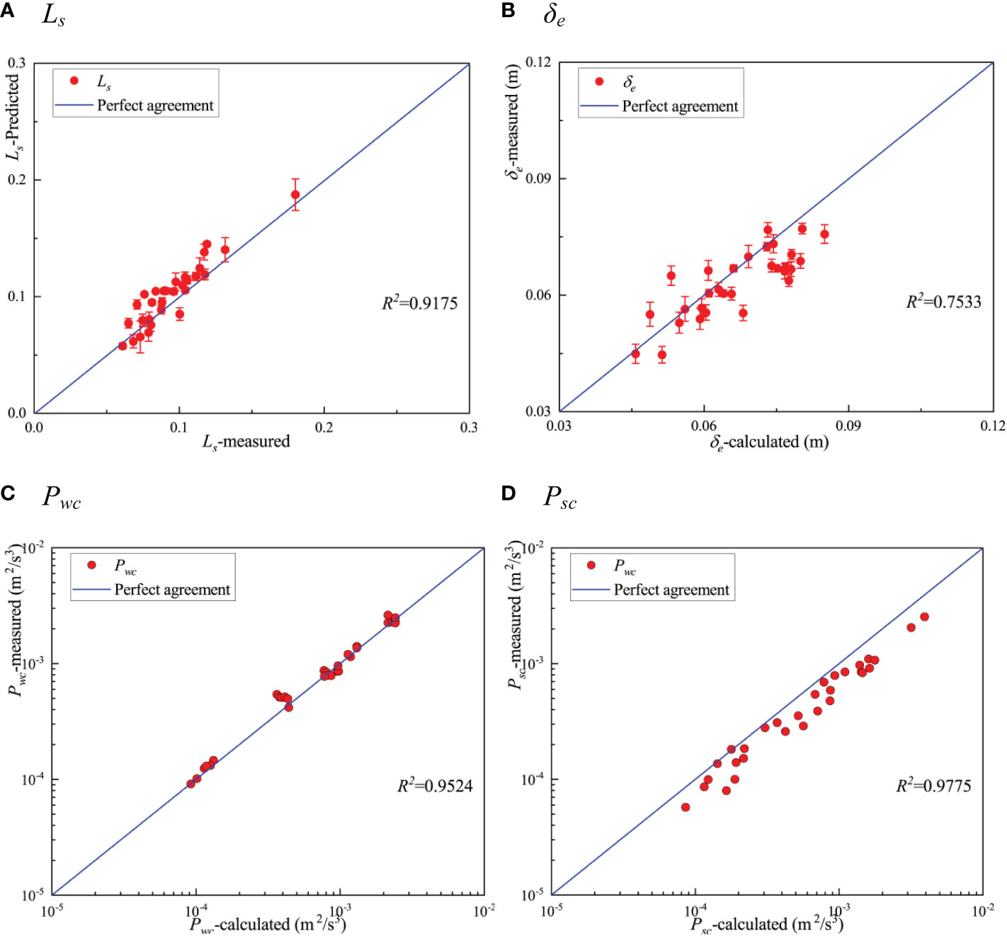
Figure 13 A comparison of predicted and measured values of shear length scale L_s (A), the penetration depth δ_e (B), vegetation canopy-averaged wake production term P_wc (C), and the vegetation canopy-averaged shear production term P_sc (D) under different test conditions.

After obtaining P_sc and P_wc, we need to find the equation for the scaling factor ξ. In general, the scaling factor, ξ, is determined based on a linear fit to the left- and right-hand side of the turbulent kinetic energy budget equation at an intercept of zero (Xu and Nepf, 2020). We used [(P_wc+P_sc)L_tc]^2/3 to perform linear fitting with k_c according to Eq. 13. Figure 14A shows the comparison between [(P_wc+P_sc)L_tc]^2/3 and k_c under different test conditions. It can be seen from the figure that [(P_wc+P_sc)L_tc]^2/3 and k_c increase with an increase in the bulk velocity, U_∞, for each vegetation material. For rigid submerged vegetation like PVC-2 and PVC-1, [(P_wc+P_sc)L_tc]^2/3 showed a linear increase with k_c and no significant change in the slope (i.e., the scaling factor, ξ), suggesting that ξ does not vary with a. These observations are in line with the study of Zhang et al. (2018). For the flexible submerged vegetation, with an increase in vegetation flexibility, the slope corresponding to k_c and [(P_wc+P_sc)L_tc]^2/3 gradually decreased, and the linear relationship was less evident than that for the rigid submerged vegetation. At the same time, when U_∞ was large, we observed some significant deviations from the fitted line (e.g., the point corresponding to E1-1), which was due to the reduction in the h_e/h_v of the vegetation at higher bulk flow velocities and a reduction in the intensity of the coherent eddies near the top of the vegetation canopy. These effects reduced the efficiency of turbulent kinetic energy production, making the increase in k_c with U_∞ smaller than the increase in [(P_wc+P_sc)L_tc]^2/3. The occurrence of this phenomenon lowers the accuracy of fitting ξ for flexible submerged vegetation using a linear formulation as compared to the accuracy of fitting it for rigid submerged vegetation. In Figure 14A, we used a linear fit to derive ξ = 0.95 ± 0.26, but the R² was only 0.66, indicating a lower accuracy of the fit.

FIGURE 14

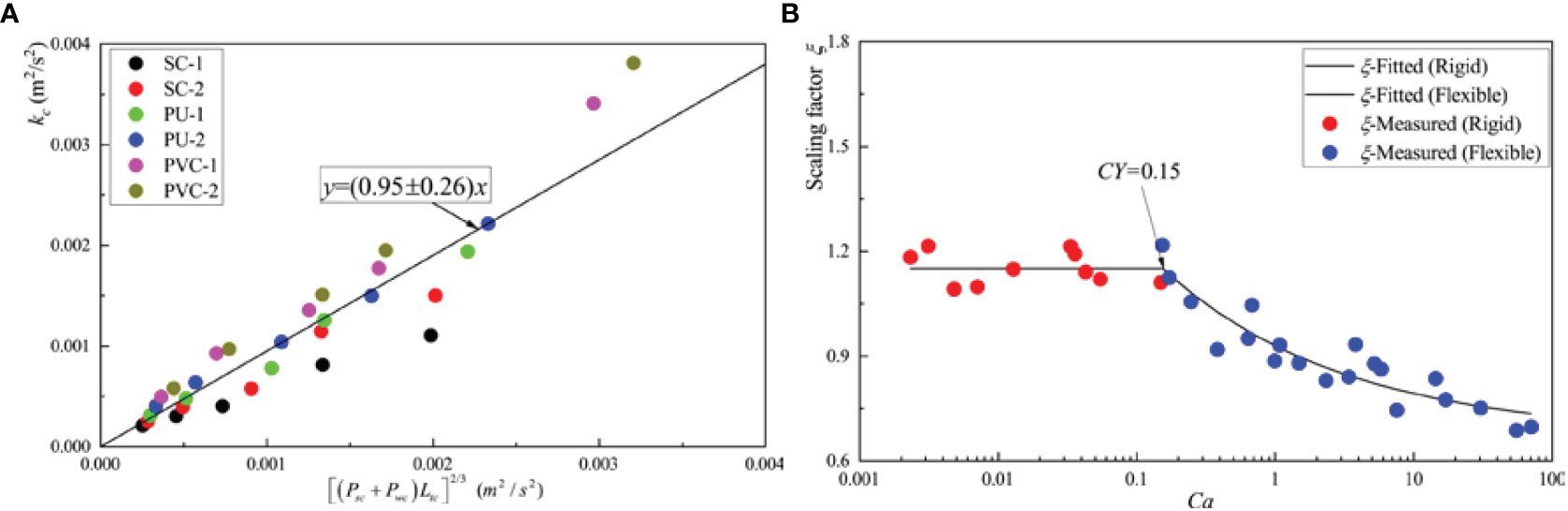
Figure 14 (A) Comparison between the vegetation canopy-averaged turbulent kinetic energy, k_c, and [(P_sc +P_wc)L_tc]^2/3. The solid black line in the figure characterizes the best fit with an intercept of 0, corresponding to a scaling factor ξ = 0.95 ± 0.26 (R² = 0.62). (B) Relationships between the scaling factor, ξ, and the Cauchy number of the vegetation canopy, Ca, under different test conditions (R² = 0.91).

Considering the possible relationship between the scaling factor, ξ, and Ca, we calculated the ξ corresponding to [(P_wc+P_sc)L_tc]^2/3 and k_c under each of the 30 test conditions in this experiment. We sorted out the relationships in Figure 14B. Among these relationships, the ξ corresponding to rigid submerged vegetation is shown in red, and ξ corresponding to the flexible submerged vegetation is shown in blue. The figure shows that for the rigid submerged vegetation, ξ did not change with Ca, and its value remained stable at around 1.15. For flexible submerged vegetation, ξ tended to decrease with increasing Ca, and the decrease leveled off, which is consistent with the report of Chen et al. (2020). There are two possible reasons for this. The first reason was the simplified prediction of the characteristic eddy length scale. We assumed that L_t = L_tc = b, which was applied to the lower part of the canopy. However, the vortex scale in the upper part of the canopy was affected not only by the wake scale turbulence but also by the coherent structure near the canopy top (Zhang et al., 2020a). Therefore, the characteristic vortex scale of rigid vegetation was higher than that of flexible vegetation (Okamoto and Nezu, 2010). This part of the prediction required a larger scaling factor to be offset. The second reason was that the model ignored the vertical transport of turbulent kinetic energy. Although many research studies have demonstrated that the vertical transport of turbulent kinetic energy is negligible as compared with wake and shear production terms, the impact of turbulent kinetic energy transport on the model still needs to be compensated by a scaling factor. This may thus be the reason why the scaling factor of rigid vegetation was greater than that of flexible vegetation.

Therefore, we took Ca = 0.15 as the Cauchy number of the critical vegetation canopy. When Ca ≦ 0.15 for rigid submerged vegetation, h_e/h_v does not change with Re_d, and produces a constant as the fitting form; when Ca≧0.15 for flexible submerged vegetation, h_e/h_v changes with Re_d. Based on the fitting method for the bulk drag coefficient of flexible submerged vegetation, we used a natural exponential relationship as the fitting form. Finally, we used the least squares method to fit the relationship between ξ and Ca, yielding the following equation:

$\begin{array}{ll}\{\begin{array}{c}\xi =1.15, Ca\le 0.15\\ \xi =0.255C{a}^{-\frac{1}{3}}+0.67, Ca\ge 0.15\end{array} & (27)\end{array}$

The coefficient of determination in Eq. 27 is R² = 0.91, which is higher than R² = 0.62 for the linear fitting approach. After obtaining the equation to determine the scaling factor, ξ, we substituted Eq. 27 into Eq. 13 to calculate the predicted values of the vegetation canopy-averaged turbulent kinetic energy k_c. Figure 15A presents the predicted values of the vegetation canopy-averaged turbulent kinetic energy, k_c, as compared with the measured values. Overall, the coefficient, R² = 0.990, for the 30 test conditions indicated high prediction accuracy, indicating that the combination of Eq. 27 and Eq. 13 can be used to reliably predict the vegetation canopy-averaged turbulent kinetic energy, k_c, under unidirectional flow with rigid or flexible submerged vegetation.

FIGURE 15

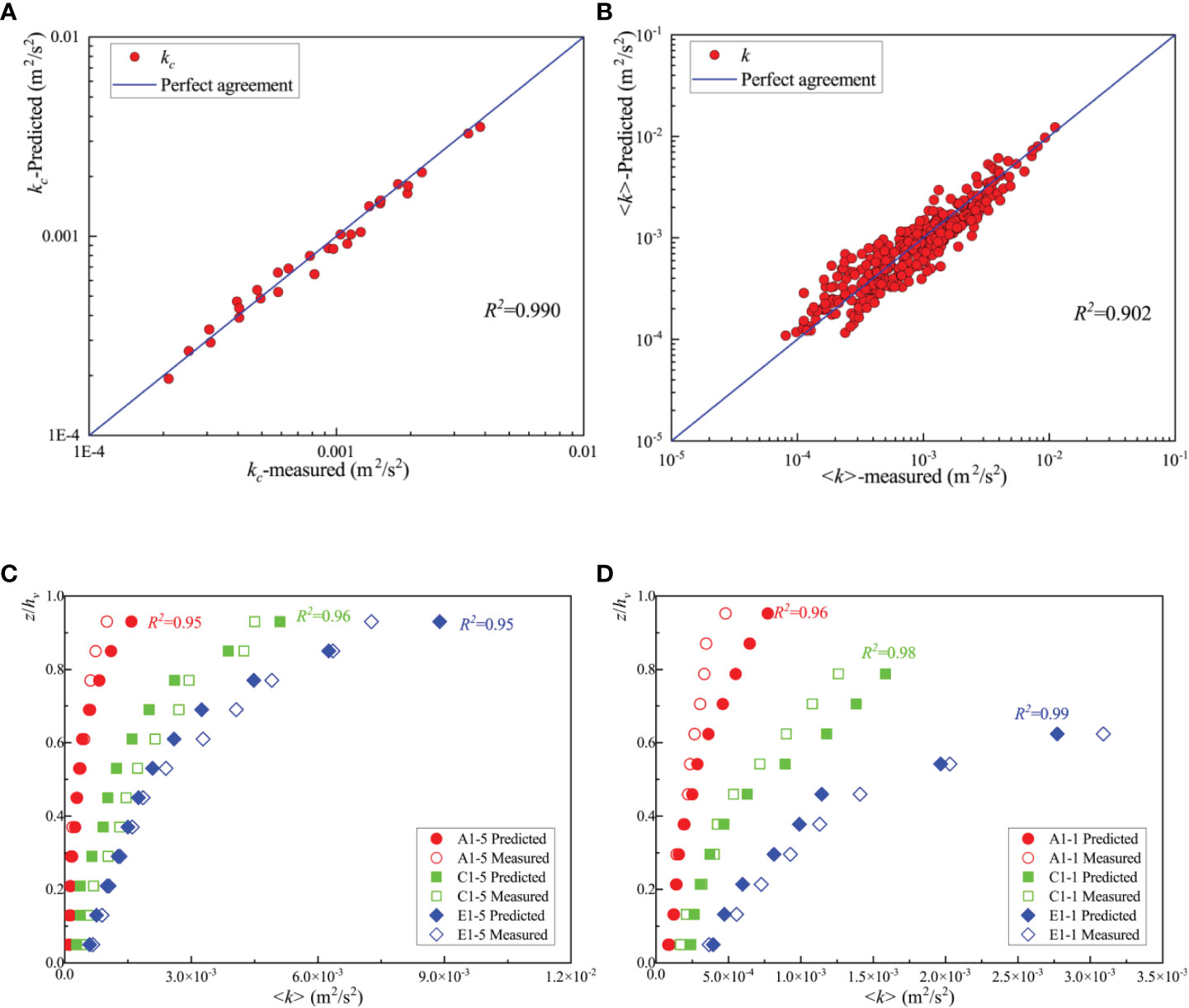
Figure 15 (A) Comparison of predicted and measured values of the vegetation canopy-averaged turbulent kinetic energy k_c; (B) comparison of the predicted and measured values of the local turbulent kinetic energy 〈k〉 within the vegetation canopy for all 30 test conditions; (C, D) comparison of predicted and measured values of the local turbulent kinetic energy 〈k〉 within vegetation canopy along the vertical direction under different tests.

To predict the local turbulent kinetic energy within the vegetation canopy, k , we assumed that the scaling factor, ξ, remains constant along the vertical direction for the same type of vegetation. We also assumed that the distribution of the local turbulent kinetic energy along the vertical direction within the vegetation canopy can be predicted by the local turbulent energy shear production term, P_s, the wake production term, P_w, and the characteristic eddy length scale, L_t. The comparison of the predicted and measured values of the local turbulent kinetic energy within the vegetation canopy for all 30 sets of test conditions is presented in Figure 15B; here, R² = 0.911, indicating high accuracy of prediction.

Figures 15C, D show the predicted distribution of local turbulent kinetic energy within the vegetation canopy under six typical test conditions. The largest error along the vertical direction is located near the vegetation canopy top. Overall, the minimum coefficient of determination for the six characteristic working conditions was 0.92, indicating that the combination of Eq. 27 and Eq. 14 can be used to predict the vertical distribution of the local turbulent kinetic energy within the rigid or flexible submerged vegetation canopy under unidirectional flow.

However, the prediction model has some limitations. The first is the method of determining the characteristic eddy length scale, L_t, and the vegetation canopy-averaged characteristic eddy length scale, L_tc (Tanino and Nepf, 2008b). This method applies to vegetation, where the frontal area of vegetation remains constant along the vertical direction, but not to natural vegetation with complex morphology. The latter type of vegetation may correspond to a gradual change in L_t along the vertical direction due to complex body variations (Caroppi et al., 2019). The second limitation is that since the buoyancy parameter, B, is less than 1 for all test conditions, its effect on the resilience of the model vegetation was neglected in this experiment. For vegetation with low stiffness and density relative to pure water, B can have a significant effect on the deflected height ratio, h_e/h_v, hydrodynamic properties, and turbulence characteristics (Zhang et al., 2020b). In such cases, the bulk drag coefficient, C_d, and scaling factor, ξ, may be related not only to Ca but also to B. In addition, since the 2D-PIV was used for measurements in this experiment, the radial (y-direction) velocity was not considered, and thus, the calculated turbulent kinetic energy is expected to be different from the turbulent kinetic energy calculated using three-dimensional instruments, such as ADV, which may also introduce error.

6 Conclusion

In this paper, the vertical distributions of velocity, Reynolds stress, drag coefficient, and turbulent kinetic energy of strip-like model vegetation with different flexibilities were measured experimentally under unidirectional flow. The research shows that with the gradual decrease in the deflection height of vegetation, the dimensionless velocity difference, Δu/U_∞ , the dimensionless mixed layer thickness, T_ml/H, the bulk drag coefficient, C_d, the vegetation canopy-averaged turbulent kinetic energy, k_c, and the vegetation canopy-averaged contribution rate of shear production term of turbulent kinetic energy, R_s/T, also decrease. The trend of penetration depth of Reynolds stress, δ_e/h_e, is the opposite. Based on the turbulent kinetic energy budget equation, a TKE model was established in this study that can be used to predict the shear production term of turbulent kinetic energy, as well as the turbulent kinetic energy within the vegetation canopy. Here, the scaling factor, ξ, is determined by the Cauchy number of the vegetation canopy, Ca. The TKE model can accurately predict the vegetation canopy-averaged and local turbulent kinetic energy within the vegetation canopy under unidirectional flow, where we are dealing with submerged vegetation of different flexibilities. Therefore, the model can be used as a simple method to predict vegetation-induced turbulence, as well as the characteristics of sediment and material transport, under the influence of submerged vegetation with different flexibility.

Data availability statement

The original contributions presented in the study are included in the article, further inquiries can be directed to the corresponding authors.

Author contributions

All authors listed have made a substantial, direct, and intellectual contribution to the work, and approved it for publication.

Funding

This work was supported by the National Natural Science Foundation of China (Grant No. 52209032) and the Natural Science Foundation of Jiangsu Province, China (Grant No. BK20200160).

Conflict of interest

The authors declare that the research was conducted in the absence of any commercial or financial relationships that could be construed as a potential conflict of interest.

Publisher’s note

All claims expressed in this article are solely those of the authors and do not necessarily represent those of their affiliated organizations, or those of the publisher, the editors and the reviewers. Any product that may be evaluated in this article, or claim that may be made by its manufacturer, is not guaranteed or endorsed by the publisher.

References

Abdolahpour M., Ghisalberti M., Mcmahon K., Lavery P. (2020). Material residence time in marine canopies under wave-driven flows. Front. Mar. Sci. 7, 574. doi: 10.3389/fmars.2020.00574

CrossRef Full Text | Google Scholar

Albayrak I., Nikora V., Miler O., O’Hare M. (2011). Flow-plant interactions at a leaf scale: Effects of leaf shape, serration, roughness and flexural rigidity. Aquat. Sci. 74 (2), 267–286. 10.1007/s00027-011-0220-9

Google Scholar

Bailey B. N., Stoll R. (2016). The creation and evolution of coherent structures in plant canopy ows and their role in turbulent transport. J. Fluid Mechanics 789, 425–460. doi: 10.1017/jfm.2015.749

CrossRef Full Text | Google Scholar

Beudin A., Kalra T., Ganju N., Warner J. C. (2017). Development of a coupled wave-flow-vegetation interaction model. Comput. Geosciences 100 (2017), 76–86. doi: 10.1016/j.cageo.2016.12.010

CrossRef Full Text | Google Scholar

Brunet Y., Finnigan J., Raupach M. R. (1994). A wind tunnel study of air flow in waving wheat: Single-point velocity statistics. Boundary-Layer Meteorology 70 (1), 95–132. doi: 10.1007/BF00712525

CrossRef Full Text | Google Scholar

Caroppi G., Västilä K., Järvelä J., Rowiński P. M., Giugni M. (2019). Turbulence at water-vegetation interface in open channel flow: Experiments with natural-like plants. Adv. Water Resour. 127, 180–191. doi: 10.1016/j.advwatres.2019.03.013

CrossRef Full Text | Google Scholar

Chen Z., Jiang C., Nepf H. (2013). Flow adjustment at the leading edge of a submerged aquatic canopy. Water Resour. Res. 49 (9), 5537–5551. doi: 10.1002/wrcr.20403

CrossRef Full Text | Google Scholar

Chen M., Lou S., Liu S., Ma G., Liu H., Zhong G., et al. (2020). Velocity and turbulence affected by submerged rigid vegetation under waves, currents and combined wave–current flows. Coast. Eng. 159 (5), 103727. doi: 10.1016/j.coastaleng.2020.103727

CrossRef Full Text | Google Scholar

Devi T. B., Kumar B. (2016). Channel hydrodynamics of submerged, flexible vegetation with seepage. J. Hydraulic Eng. 142 (11), 04016053. doi: 10.1061/(ASCE)HY.1943-7900.0001180

CrossRef Full Text | Google Scholar

Dijkstra J., Uittenbogaard R. (2010). Modeling the interaction between flow and highly flexible aquatic vegetation. Water Resour. Res. 46 (12), 1–12. doi: 10.1029/2010WR009246

CrossRef Full Text | Google Scholar

Ellington C. P. (1991). Aerodynamics and the origin of insect flight. Adv. Insect Physiol. 23, 171–210. doi: 10.1016/S0065-2806(08)60094-6

CrossRef Full Text | Google Scholar

Etminan V., Lowe R., Ghisalberti M. (2017). A new model for predicting the drag exerted by vegetation canopies. Water Resour. Res. 53 (4), 3179-3196. doi: 10.1002/2016WR020090

CrossRef Full Text | Google Scholar

Finnigan J. (2000). Turbulence in plant canopies. Annu. Rev. Fluid Mechanics 32, 519–571. doi: 10.1146/annurev.fluid.32.1.519

CrossRef Full Text | Google Scholar

Ghisalberti M. (2009). Obstructed shear flows: Similarities across systems and scales. J. Fluid Mechanics 641, 51–61. doi: 10.1017/S0022112009992175

CrossRef Full Text | Google Scholar

Ghisalberti M., Nepf H. M. (2001). Mixing layers and coherent structures in vegetated aquatic flows. J. Geophysical Res. 107 (C2), 1–11. doi: 10.1029/2001JC000871

CrossRef Full Text | Google Scholar

Ghisalberti M., Nepf H. M. (2004a). The limited growth of vegetated shear layers. Water Resour. Res. 40 (W07502), 1-12. doi: 10.1029/2003WR002776

CrossRef Full Text | Google Scholar

Ghisalberti M., Nepf H. M. (2004b). The limited growth of vegetated shear layers. Water Resour. Res. 40 (7), 1–12. doi: 10.1029/2003WR002776

CrossRef Full Text | Google Scholar

Ghisalberti M., Nepf H. (2006). The structure of the shear layer in flows over rigid and flexible canopies. Environ. Fluid Mechanics 6 (3), 277–301. doi: 10.1007/s10652-006-0002-4

CrossRef Full Text | Google Scholar

Huai W.-x., Li S., Katul G. G., Liu M.-Y., Yang Z.-H. (2021). Flow dynamics and sediment transport in vegetated rivers: A review. J. Hydrodynamics 33 (3), 400–420. doi: 10.1007/s42241-021-0043-7

CrossRef Full Text | Google Scholar

Hu Z., Lei J., Liu C., Nepf H. M. (2018). Wake structure and sediment deposition behind models of submerged vegetation with and without flexible leaves. Adv. Water Resour. 118 (8), 28–38. doi: 10.1016/j.advwatres.2018.06.001

CrossRef Full Text | Google Scholar

Jamali M., Sehat H. (2020). Experimental study of lateral dispersion in flexible aquatic canopy with emergent blade-like stems. Phys. Fluids 32 (6), 067116. doi: 10.1063/5.0010665

CrossRef Full Text | Google Scholar

King A. T., Tinoco R. O., Cowen E. A. (2012). A k-epsilon turbulence model based on the scales of vertical shear and stem wakes valid for emergent and submerged vegetated flows. J. Fluid Mechanics 701, 1–39. doi: 10.1017/jfm.2012.113

CrossRef Full Text | Google Scholar

Kouwen N., Li R.-M. (1980). Biomechanics of vegetative channel linings. Am. Soc. Civil Engineers 106 (6), 1085–1103. doi: 10.1061/JYCEAJ.0005444

CrossRef Full Text | Google Scholar

Kouwen N., Moghadam M. F. (2000). Friction factors for coniferous trees along rivers. J. Hydraulic Eng. 126 (10), 732–740. doi: 10.1061/(ASCE)0733-9429(2000)126:10(732)

CrossRef Full Text | Google Scholar

Lei J., Nepf H. M. (2019). Blade dynamics in combined waves and current. J. Fluids Structures 87, 137–149. doi: 10.1016/j.jfluidstructs.2019.03.020

CrossRef Full Text | Google Scholar

Lei J., Nepf H. M. (2021). Evolution of flow velocity from the leading edge of 2-d and 3-d submerged canopies. J. Fluid Mechanics 916, 1-27. doi: 10.1017/jfm.2021.197

CrossRef Full Text | Google Scholar

Liu M.-Y., Huai W.-X., Zhong-Hua Yang and Zeng Y.-H. (2020). A genetic programming-based model for drag coefficient of emergent vegetation in open channel flows. Adv. Water Resour. 140 1–10. doi: 10.1016/j.advwatres.2020.103582

CrossRef Full Text | Google Scholar

Liu C., Shan Y., Heidi M N. (2021). Impact of stem size on turbulence and sediment resuspension under unidirectional flow. Water Resour. Res. 57, e2020WR028620. doi: 10.1029/2020WR028620

CrossRef Full Text | Google Scholar

Liu C., Yan C., Sun S., Lei J., Nepf H., Shan Y. (2022). Velocity, turbulence and sediment deposition in a channel partially filled with a phragmites australis canopy. Water Resour. Res 58, 1-21. doi: 10.1029/2022WR032381

CrossRef Full Text | Google Scholar

Liu J., Zhang Z., Yu Z., Liang Y., Li X., Ren L. (2017). The structure and flexural properties of typha leaves. Appl. Bionics Biomechanics, 1–9. doi: 10.1155/2017/1249870

CrossRef Full Text | Google Scholar

Li Y., Wang Y., Anim D. O., Tang C., Du W., Ni L., et al. (2014). Flow characteristics in different densities of submerged flexible vegetation from an open-channel flume study of artificial plants. Geomorphology 2014, 314–324. doi: 10.1016/j.geomorph.2013.08.015

CrossRef Full Text | Google Scholar

Li Y.-H., Xie L., Su T.-C. (2018). Resistance of open-channel flow under the effect of bending deformation of submerged flexible vegetation. J. Hydraulic Eng. 144 (3), 04017072. doi: 10.1061/(ASCE)HY.1943-7900.0001419

CrossRef Full Text | Google Scholar

López F., García M. H. (1998). Open-channel flow through simulated vegetation: Suspended sediment transport modeling. Water Resour. Res. 34 (9), 2341–2352. doi: 10.1029/98WR01922

CrossRef Full Text | Google Scholar

Luhar M., Nepf H. M. (2011). Flow-induced reconfiguration of buoyant and flexible aquatic vegetation. Limnology Oceanography 56, 2003–2017. doi: 10.4319/lo.2011.56.6.2003

CrossRef Full Text | Google Scholar

Morris E. P., Peralta G., Brun F. G., Duren L., Bouma T. J., Pérez-Lloréns J. L. (2008). Interaction between hydrodynamics and seagrass canopy structure: Spatially explicit effects on ammonium uptake rates. Limnology Oceanography 53 (4), 1531–1539. doi: 10.4319/lo.2008.53.4.1531

CrossRef Full Text | Google Scholar

Nepf H. M. (2011). Flow and transport in regions with aquatic vegetation. Annu. Rev. Fluid Mechanics 44, 123–142. doi: 10.1146/annurev-fluid-120710-101048

CrossRef Full Text | Google Scholar

Nepf H. M. (2012). Hydrodynamics of vegetated channels. J. Hydraulic Res. 50 (3), 262–279. doi: 10.1080/00221686.2012.696559

CrossRef Full Text | Google Scholar

Nepf H. M., Vivoni E. (2000). Flow structure in depth-limited, vegetated flow. J. Geophysical Res. 105 (C12), 28547–28557. doi: 10.1029/2000JC900145

CrossRef Full Text | Google Scholar

Neumeier U. (2007). Velocity and turbulence variations at the edge of saltmarshes. Continental Shelf Res. 27 (8), 1046–1059. doi: 10.1016/j.csr.2005.07.009

CrossRef Full Text | Google Scholar

Nezu I., Sanjou M. (2008). Turburence structure and coherent motion in vegetated canopy open-channel flows. J. Hydro-environment Res. 2 (2), 62–90. doi: 10.1016/j.jher.2008.05.003

CrossRef Full Text | Google Scholar

Nikora V., McEwan I., Mclean S. R., Coleman S., Pokrajac D., Walters R. A. (2007). Double-averaging concept for rough-bed open-channel and overland flows: Theoretical background. J. Hydraulic Eng. 133 (8), 873–883. doi: 10.1061/(ASCE)0733-9429(2007)133:8(873)

CrossRef Full Text | Google Scholar

Okamoto T.-A., Nezu I. (2010). Turbulence structure and “Monami” phenomena in flexible vegetated open-channel flows. J. Hydraulic Res. 47 (6), 798–810. doi: 10.3826/jhr.2009.3536

CrossRef Full Text | Google Scholar

Okamoto T., Nezu I., Sanjou M. (2016). Flow–vegetation interactions: Length-scale of the “monami” phenomenon. J. Hydraulic Res. 54 (3), 251–262. doi: 10.1080/00221686.2016.1146803

CrossRef Full Text | Google Scholar

Park H., Hwang J. H. (2019). Quantification of vegetation arrangement and its effects on longitudinal dispersion in a channel. Water Resour. Res. 55, 1–11. doi: 10.1029/2019WR024807

CrossRef Full Text | Google Scholar

Raupach M. R., Shaw R. H. (1982). Averaging procedures for flow within vegetation canopies. Boundary-Layer Meteorology 22 (1), 79–90. doi: 10.1007/BF00128057

CrossRef Full Text | Google Scholar

Rominger J. T., Nepf H. M. (2014). Effects of blade flexural rigidity on drag force and mass transfer rates in model blades. Limnology Oceanography 59 (6), 2028–2041. doi: 10.4319/lo.2014.59.6.2028

CrossRef Full Text | Google Scholar

Sonnenwald F., Stovin V., Guymer I. (2018). Estimating drag coefficient for arrays of rigid cylinders representing emergent vegetation. J. Hydraulic Res. 57, 1–7. doi: 10.1080/00221686.2018.1494050

CrossRef Full Text | Google Scholar

Tang C., Lei J., Nepf H. M. (2019). Impact of vegetation-generated turbulence on the critical, near-bed, wave-velocity for sediment resuspension. Water Resour. Res. 55, 1-14. doi: 10.1029/2018WR024335

CrossRef Full Text | Google Scholar

Tang X., Lin P., Liu P. L.-F., Zhang X. (2021). Numerical and experimental studies of turbulence in vegetated open-channel flows. Environ. Fluid Mechanics 21 (2), 1–27. doi: 10.1007/s10652-021-09812-7

CrossRef Full Text | Google Scholar

Tang H., Tian Z., Yan J., Yuan S. (2014). Determining drag coefficients and their application in modelling of turbulent flow with submerged vegetation. Adv. Water Resour. 69, 134–145. doi: 10.1016/j.advwatres.2014.04.006

CrossRef Full Text | Google Scholar

Tanino Y., Nepf H. (2007). Experimental investigation of lateral dispersion in aquatic canopies (Venice, Italy: 32nd International Association of Hydraulic Engineering & Research (IAHR)), 152.

Google Scholar

Tanino Y., Nepf H. M. (2008a). Laboratory investigation of mean drag in a random array of rigid, emergent cylinders. J. Hydraulic Eng. 134, 34–41. doi: 10.1061/(ASCE)0733-9429(2008)134:1(34)

CrossRef Full Text | Google Scholar

Tanino Y., Nepf H. M. (2008b). Lateral dispersion in random cylinder arrays at high reynolds number. J. Fluid Mechanics 600, 339–371. doi: 10.1017/S0022112008000505

CrossRef Full Text | Google Scholar

Tennekes H. H., Lumley J. L. (1972). A first course in turbulence (Cambridge, MA: MIT Press).

Google Scholar

Termini D. (2019). Turbulent mixing and dispersion mechanisms over flexible and dense vegetation. Acta Geophysica 67 (7), 961–970. doi: 10.1007/s11600-019-00272-8

CrossRef Full Text | Google Scholar

Thielicke W., Stamhuis E. J. (2014). PIVlab – towards user-friendly, affordable and accurate digital particle image velocimetry in MATLAB. J. Open Res. Software 2, 1-10. doi: 10.5334/jors.bl

CrossRef Full Text | Google Scholar

Tinoco R. O., Coco G. (2016). A laboratory study on sediment resuspension within arrays of rigid cylinders. Adv. Water Resour. 92, 1–9. doi: 10.1016/j.advwatres.2016.04.003

CrossRef Full Text | Google Scholar

Tseng C.-Y., Tinoco R. O. (2020). A model to predict surface gas transfer rate in streams based on turbulence production by aquatic vegetation. Adv. Water Resour. 143, 1-18. doi: 10.1016/j.advwatres.2020.103666

CrossRef Full Text | Google Scholar

Vargas-Luna A., Crosato A., Uijttewaal W. S. J. (2015). Effects of vegetation on flow and sediment transport: Comparative analyses and validation of predicting models. Earth Surface Processes Landforms 40 (2), 157–176. doi: 10.1002/esp.3633

CrossRef Full Text | Google Scholar

Veelen T., Fairchild T., Reeve D. E., Karunarathna H. (2020). Experimental study on vegetation flexibility as control parameter for wave damping and velocity structure. Coast. Eng. 157, 103648. doi: 10.1016/j.coastaleng.2020.103648

CrossRef Full Text | Google Scholar

Wang H., Cong P., Zhu Z., Zhang W., Ai Y., Huai W.-x. (2022). Analysis of environmental dispersion in wetland flows with floating vegetation islands. J. Hydrology 606 (1), 127369. doi: 10.1016/j.jhydrol.2021.127359

CrossRef Full Text | Google Scholar

Waycott M., Duarte C. M., Carruthers T. J. B., Orth R. J., Dennison W., Olyarnik S. V., et al. (2009). Accelerating loss of seagrass across the globe threatens coastal ecosystems. Proc. Natl. Acad. Sci. 106 (30), 12377–12381. doi: 10.1073/pnas.0905620106

CrossRef Full Text | Google Scholar

Wilcock R. J., Champion P. D., Nagels J., Croker G. F. (1999). The influence of aquatic macrophytes on the hydraulic and physico-chemical properties of a new Zealand lowland stream. Hydrobiologia 416 (1), 203–214. doi: 10.1023/A:1003837231848

CrossRef Full Text | Google Scholar

Wilson J. D. (1988). A second-order closure model for flow through vegetation. Boundary-Layer Meteorology 42 (4), 371–392. doi: 10.1007/BF00121591

CrossRef Full Text | Google Scholar

Xu Y., Nepf H. M. (2020). Measured and predicted turbulent kinetic energy in flow through emergent vegetation with real plant morphology. Water Resour. Res. 56 (12), e2020WR027892. doi: 10.1029/2020WR027892

CrossRef Full Text | Google Scholar

Yang J., Chung H., Nepf H. M. (2016). The onset of sediment transport in vegetated channels predicted by turbulent kinetic energy. Geophysical Res. Lett., 43 (21), 11, 261–11, 268. doi: 10.1002/2016GL071092

CrossRef Full Text | Google Scholar

Yang J., Nepf H. M. (2019). Impact of vegetation on bed load transport rate and bedform characteristics. Water Resour. Res. 55, 1-16. doi: 10.1029/2018WR024404

CrossRef Full Text | Google Scholar

Zhang J., Lei J., Huai W., Nepf H. M. (2020a). Turbulence and particle deposition under steady flow along a submerged seagrass meadow. J. Geophysical Research: Oceans 125, e2019JC015985. doi: 10.1029/2019JC015985

CrossRef Full Text | Google Scholar

Zhang S., Liu Y., Wang Z., Li G. (2019). Effect of flexible vegetation lodging on overland runoff resistance. Water Environ. J. 34 (3), 1–9. doi: 10.1111/wej.12529

CrossRef Full Text | Google Scholar

Zhang Y., Tang C., Nepf H. M. (2018). Turbulent kinetic energy in submerged model canopies under oscillatory flow. Water Resour. Res. 54, 1734–1750. doi: 10.1002/2017WR021732

CrossRef Full Text | Google Scholar

Zhang Y., Wang P., Cheng J., Wang W.-J., Zeng L., Wang B. (2020b). Drag coefficient of emergent flexible vegetation in steady nonuniform flow. Water Resour. Res. 56 (8), e2020WR027613. doi: 10.1029/2020WR027613

CrossRef Full Text | Google Scholar

Zimmerman R. C. (2003). A biooptical model of irradiance distribution and photosynthesis in seagrass canopies. Limnology Oceanography 48(1 Part 2), 568–585. doi: 10.4319/lo.2003.48.1_part_2.0568

CrossRef Full Text | Google Scholar