Wind effect on sediment suspensions over silt-dominated mixtures: An experimental study

A series of laboratory experiments have been conducted to explore the wind effect on Sediment Suspended Concentrations (SSCs) in fine-grained coastal systems. The paddle waves were overplayed with surface-blowing winds in a wind-wave flume to mimic offshore swells coupling with local wind waves during rough weather. Both SSCs and water turbulences under different wind and wave conditions have been investigated over two kinds of sediment beds (Sediment 1, S1, D₅₀ = 52µm and Sediment 2, S2, D₅₀ = 90µm). The High Concentration Layers (HCL) were formed under most of the wave-only conditions, while with the introduction of the stronger wind, more sediment suspensions were transported upward, increasing SSCs in upper water elevations. The finer sediment S1 is easier to suspend than S2 under the same conditions. The enhancement of the vertical turbulence intensity (σ_w) by winds is the main reason for the increase in SSCs. Meanwhile, because the wind-induced turbulence can hardly penetrate the HCL, the turbulence intensities outside the HCL can be further amplified compared to the experiment without a sediment bed. The wind contributes over 65% of the SSC enlargement above the HCL under a wind of 10m/s for S1, while less than 20% inside the HCL in most wind conditions. The sediment mixing coefficient (ϵ_s), a crucial parameter for suspended sediment modeling, was enhanced with stronger winds. Although the existing formulas for the vertical distribution of ϵ_s are valid under both wave-only and small winds (2.5 m/s) for both sediment beds, the enhancement of ϵ_s caused by strong winds cannot be captured, requiring further research.

1. Introduction

Sediment transport has a marked influence on coastal physical processes linking feedback loops between hydrodynamics (e.g., current, wave), turbulence, and morphological evolution (Bailey and Hamilton, 1997; Wu and Hua, 2014). In shallow areas abundant in fine sediments, such as estuaries and tidal flats, the suspended load is the primary means of sediment transport. Meanwhile, suspended sediments are important agents carrying organic matter, nutrients, heavy metals, and other substances in estuarine and coastal waters, which affect coastal environmental processes (Green and Coco, 2014; Tao et al., 2020). Therefore, understanding suspended sediment dynamics is substantial for coastal morphology and ecological evolution (Cloern, 1987; Liu et al., 2014).

Sediment suspensions are primarily dependent on the turbulent motions in shallow waters, which are produced by single or combined interactions between various hydrodynamics, such as waves, currents, and winds (Bailard, 1981; Hassan and Ribberink, 2005; van Rijn, 2007; Kobayashi et al., 2008; Aagaard and Hughes, 2010; Kassem et al., 2015; Alsina et al., 2018). Bailard (1981) reported that the oscillatory wave motions performed the essential action to transport the sediment on the sandy coast. O’ Hara Murray et al. (2012) reported that the wave groups, compared to a single incident wave, could generate over three times more surficial SSCs. The wave groups with varying wave heights are more active in suspending and entraining the bed sediment. Alsina et al. (2018) presented that the short-wave groups induced sediment suspended transport is dominated by horizontal advection with significant wave-swash interactions. Kassem et al. (2015) demonstrated that wave motion plays an important role in entraining sediment inside the boundary layer and high-frequency turbulence due to the momentum transfer into smaller scales supports the particles in suspension. Furthermore, Pang et al. (2020) revealed that the TKE contributed more effectively to sediment suspension at the scale of wave group than that of the incident wave, especially under broken wave conditions. Meanwhile, some research focuses on sediment suspension under complex dynamics. For example, Yao et al. (2015) conducted a series of flume experiments to explore the sediment suspension behavior under the wave and current conditions over sand-silt mixtures, discovering that current velocity can prompt the sediment suspension in upper layers compared to the wave-only condition. Meanwhile, the current direction does not significantly affect the time-averaged concentration profiles. Furthermore, much work has been done in some wind-dominated areas to explore the relationship and mechanism between wind and sediment suspension concentrations (Bailey and Hamilton, 1997; Booth et al., 2000; Su et al., 2015; Pu et al., 2022).

Apart from turbulent motions induced by various coastal hydrodynamics, the properties of sediment particles themselves, such as particle size, cohesion, and bed composition, also exert influence on sediment suspensions (van Rijn, 1989; Van Rijn et al., 1993; Mitchener and Torfs, 1996; Jacobs et al., 2011). For example, Van Rijn et al. (1993) reported that the vertical mixing process of fine sand (D₅₀ = 200μm) suspension could be significantly reinforced in current and wave conditions. However, for cohesive sediment, different behaviors can be observed. Flume experiments with a wave over a consolidated mud bed have shown that the top-layer mud can be easily fluidized, generating a thin layer with large concentrations near the bottom (Maa and Mehta, 1987; Van Rijn and Louisse, 1987). Moreover, several studies have paid attention to the behavior of mixed sediment in order to predict mixed sediment transport (van Ledden et al., 2006; Sanford, 2008). Based on a validated fine sediment transport model, Waeles et al. (2008) proposed that the relative mud concentration determines the critical bed shear stress for the erosion of the superficial sediment. In addition, silt, whose size is located between sand and clay, is widely distributed in China, such as the tidal flat along the central Jiangsu coast and the modern Yellow River Delta (Gong et al., 2017; Xu et al., 2018). Silty sediment has been shown to have both cohesive and non-cohesive properties, attracting the attention of many scholars (Yao et al., 2015, Yao et al., 2022a; Yao et al., 2022b; Zuo et al., 2017; Zuo et al., 2021).

Regarding the dynamic behavior of suspension enriched in silty sediments, Zhao (2003) reported that when the cohesive fraction is low, three sediment motion forms can be identified (i.e., bed load, near-bottom high concentration layers, and suspended load in upper layers). Otherwise, the sediment transport is mainly in the suspended load. Yao et al. (2015) recognized that silty suspensions have different concentration profiles from sand under wave-only and wave-with-current conditions, respectively. Under wave-only conditions, a high concentration layer (HCL) can be formed. Inside the HCL, the silt concentration decreases logarithmically (sand-like behavior), whereas the concentration profile is distributed homogeneously outside the HCL (clay-like behavior). Zuo et al. (2021) updated existing formulations for the sand-silt mixtures to estimate depth-averaged SSCs for both vortex-rippled beds and sheet flow conditions. Several basic physical processes have been considered, such as stratification, hindered settling, and mobile beds.

It is believed that wave motion is the primary form of energy transference during wind blowing, which plays a significant role in maintaining suspensions. In addition to wave motion, Su et al. (2015) found that wind can enhance SSC directly by exerting turbulence into the water using wind-flume experiments. Furthermore, Zhu et al. (2016) found that wind would affect water turbulence in another way besides wave orbital motions based on in-situ field observations. Therefore, only applying wave-induced bed shear stress and mixing coefficient cannot interpret the enhancement of SSCs in a silt-dominated system during rough weather. Whether surface-generated turbulence by wind directly influences water turbulence structures, mixing processes, and thus the SSC distribution is unclear.

This study aims to explore the wind effect on fine sediment suspensions over silt-dominated mixtures. A series of experiments have been carried out in a wind-wave flume with two types of sediments under different wind and paddle wave conditions (i.e., offshore swells combined with the local wind). The addressed research questions include: (1) to what extent the wind will affect silt suspensions in shallow areas; (2) how the wind affects the mixing processes of suspended silty particles and the vertical distribution of SSCs. Section 2 describes the experimental setup, instrumentation, and analysis methods, followed by the result analyses in Section 3, including vertical distributions of SSCs and the turbulence intensities under different experimental conditions. Section 4 provides discussions followed by conclusions in Section 5.

2. Methods

2.1. Flume experiment

The laboratory experiments were performed in a wind-wave flume at Hohai University, China. The flume has a length of 80m, a width of 1m, and a depth of 1m (Figure 1). Sediment samples used in this experiment were collected from a silt-rich tidal flat in the middle of the Jiangsu coast, China. Our sampling fieldwork was carried out in mid-August 2018, and two sediment samples from the tidal flat were collected: Sediment 1 (referred to as S1) from the upper flat and Sediment 2 (referred to as S2) from the middle flat. The particle sizes of the samples (S1 and S2) were measured by a Malvern Mastersize 3000 laser particle size analyzer. S1 is a silt-enriched mixture (70% of silt content; D₅₀ = 52µm) while S2 is a very fine sand-enriched mixture (30% of silt content; D₅₀ = 90µm). The measured particle size distributions of the two bed sediments are shown in Figure 2.

FIGURE 1

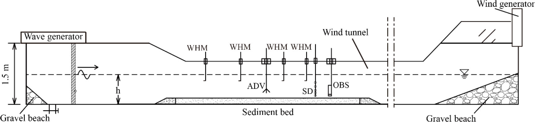
Figure 1 The experimental design and schematic of the wind-wave flume.

FIGURE 2

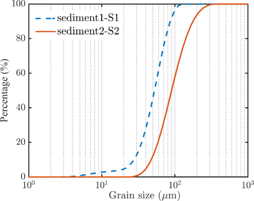
Figure 2 The particle size distributions of the two bed sediments.

The layout of the experimental flume, such as the wave generator, suction fan, and wave dissipator, is illustrated in Figure 1. The wave generator is located upstream of the flume, and three wave height probes are placed on the wave paddle to detect the reflected wave. By automatically adjusting the position of the wave paddle, the reflected wave can be minimized. The gravel beach slope, with a slope of 1:4.5, was also set downstream. In this study, a typical experiment duration is around 2 hours, including the time to achieve a steady state of SSC and the data collection. The active and passive wave reflection absorption systems can guarantee wave stability during long-time wave generation. Since this study focuses on SSC profiles during a steady state, the stability of the wave is essential for the measurement. Meanwhile, wave reflection is inevitable during long-time wave generation. Thus, the waves at the sediment section are combinations of the incident and reflected waves, which show a similar shape as Stokes second-order waves (See Figure S1 in Supplementary Materials). The 2nd Stokes wave represents the function of wave reflection. Therefore, the separation of wave reflection is not our primary concern. The reflection coefficients of paddle wave experiments are around 0.0626-0.2713 (based on 3-gauge method of Mansard and Funke (1980) and 0.0647-0.2034 (based on a time domain method of Sun et al. (2002)). See Table S1 in the Supplementary Materials for details. Furthermore, the present experiment methodology is consistent with existing studies on SSCs in the wave flume (such as, van Rijn and Kroon, 1992; Thorne, 2002; Yao et al., 2015; Davies and Thorne, 2016).

A suction fan was installed on the downstream side of the flume to produce wind in the same direction as waves. The wind covers were fixed on the top of the flume. Before experimenting with a sediment bed in this study, we have also done a series of experiments with a fixed bed (namely, sediment-free experiment; SFE hereinafter), keeping other experimental settings unchanged. The SFE mainly focused on wind effects on water turbulence, which showed that the surface-blowing wind intensified the turbulent kinematic energy (TKE) in the upper water column in addition to wave orbital motions.

Four Wave Height Meters (WHMs) were installed along the flume to measure the water surface elevation (Figure 1). The instantaneous water velocity was measured by the Acoustic Doppler Velocimeter (ADV). The ADV was mounted on a mobile measuring frame that can be moved vertically by a computer control system. Seven measurement points were arranged along the beam, the lowest one was 0.6 cm above the bottom, the highest one was at Z=0.6h (h is the water depth), and the other 5 points were placed at every 0.1h in between. The sampling rate was set to 50Hz. It should be noted that the velocity signal near the water surface, which is a blind area of the ADV, cannot be recorded. Nevertheless, substance mixing (e.g., sediment suspension) was more pronounced in the middle and lower water column. Therefore, the velocities in the middle and lower layers were analyzed and investigated in this study. The wind speed was measured by a hot-wire anemometer placed 350 mm above the motionless water surface.

Two Optical Backscatter Sensors (OBS 3+) were mounted vertically on another mobile measuring frame with a 35mm interval, providing the real-time signals on SSC development. The lens of the OBS was adjusted to be parallel to the wave direction. The initial position of the lower OBS was placed about 5 mm above the sediment bed. Our previous study has proved that the OBS signal was positively related to SSC when SSC< 40g/l (Su et al., 2016). Thus, when the OBS signal reached a steady state, the stable state of the water SSC was considered to be achieved and another function of OBS is to help us check the quality of the water SSC values during the data process. Subsequently, a specially designed siphon device was applied for the water-sediment sampling to obtain time-averaged SSC. Comparison between time-averaged OBS signals and time-averaged SSC shows a quadratic relationship, suggesting a good data quality of SSC measured by the siphon device. See Figure S2 in the Supplementary Materials for more information on OBS and SSC calibration curves. Meanwhile, the ADV started to record the velocity data as well. The siphon device (SD in Figure 1) was mounted at the left of the OBS frame at a horizontal distance of 0.6m. The lowest intake tube was set initially at 1 cm above the original flat sediment bed. During the experiment, the local bed forms were developed so that the relative height of the siphon device (i.e., SSC of each elevation) as well as the velocity data from ADV was corrected correspondingly according to the mean bed level (average of the ripple crests and troughs). Thus, under different experimental conditions, each intake tube’s vertical positions differed. In each experimental case, the sediment samples were taken twice with a time interval of 10 minutes and were put into six pre-calibrated pycnometers and six glass cylinders, respectively. For the glass cylinders, the samples had to be filtered, dried and weighted to attain the time-averaged sediment concentration. For samples in the pre-calibrated pycnometers, the concentration can be calculated by weighting directly. Each experimental group was repeated twice. By averaging the two concentrations of repeated experiments, the final SSC of each experimental group can be obtained.

2.2. Experimental conditions

Instead of mimicking the field conditions on an accurate natural scale, the present study utilizes a series of controllable flume experiments with various designs. Different combinations of winds (wind speed of 0–10 m/s) and regular waves (wave heights of 6–14 cm) were designed for the experiment. The water depth (h) was 0.3m, and the wave period was kept constant, i.e., T=1.5s. Based on different experimental conditions, the resulting bed shear stresses and turbulence intensities which are important for SSCs, should be comparable to the field conditions. By these designs, the bed shear stress over the sediment bed varies in a range of 0.26-0.59 Pa over sediment S1 and 0.28-0.62 Pa over sediment S2. The bed shear stress was calculated following van Rijn (2007) by the measured near bed orbital velocity, wave period, water depth, and sediment particle size (D₅₀). The turbulence intensities (horizontal) in the laboratory are in the range of 0-0.03 m/s (details refer to section 3.2), In the tidal flat, the typical bed shear stress during windy conditions is around 0~0.8 Pa (Mariotti and Fagherazzi, 2013; Zhu et al., 2016; Hu et al., 2017), and the turbulence intensities are in the range of 0-0.06 m/s (Soulsby and Humphery, 1990). Thus, the representativeness of our experimental designs for the field conditions can be well validated.

Several pre-experimental tests have been conducted under wind-only and paddle wave-only conditions, respectively. The paddle wave shows a relatively regular shape and a narrow frequency band (see Figure S3 in the Supplementary Materials). The wave induced by surface-blowing wind depicts a wide frequency band with irregular shapes. Under 6 m/s pure wind conditions, the wave heights measured in the sediment section are around 1.77-1.93 cm, and the wave periods are 0.33-0.37s. Thus, the features of the paddle wave and wind-blowing wave generated in the flume are consistent with that of swells and wind waves in the field. In the following, the paddle wave is named swell, and the wind-blowing wave is named wind-wave, following previous studies, such as Cheng and Mitsuyasu (1992) and Mitsuyasu and Yoshida (2005).

Details of other experimental conditions are listed in Table 1. The capital letters (A, B, C) represent the experimental cases (i.e., wave height, H = 6cm, 10cm, 14cm) and the numbers represent the corresponding wind speed level. Four levels of wind speed are designed, i.e., 0, 2.5, 6, and 10m/s. For example, S1A3 represents the experimental case with sediment S1 under a wave of 6cm and a level 3 wind speed (i.e., 10m s^-1). As mentioned before, the waves generated by wind only are tiny, and no sediment is initiated into motion. Therefore, the experimental conditions do not include wind-only conditions. The impacts of wind-induced turbulence on the sediment suspension can be obtained by comparing SSCs under wave-only and wave-wind combined conditions. Subsequently, the relative contribution of wind-induced and wave-induced turbulence on SSC under different conditions can be deduced.

TABLE 1

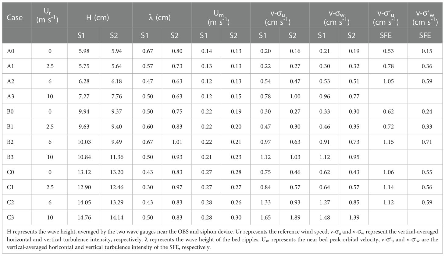
Table 1 Basic measurements and derived data for S1 and S2.

2.3. Data analyses

The data analyses in the present study include the vertical distributions of the SSC, the calculation of turbulence parameters of the water column as well as the sediment mixing coefficient. For the vertical distributions of SSC, the method has been described in 2.1. The turbulence component needs to be separated from the original velocity signal to get the turbulence intensity. Then, the horizontal intensity σ_u and the vertical intensity σ_w can be calculated.

The instantaneous water velocities in horizontal and vertical directions are typically divided into:

$\begin{array}{ll}u=\overline{u}+\tilde{u}+u\text{′}& (1)\end{array}$

$\begin{array}{ll}w=\overline{w}+\tilde{w}+w\text{′}& (2)\end{array}$

where u and w are the instantaneous velocity in the horizontal and vertical direction, respectively; $\overline{u} \text{and} \overline{w}$ are the time-averaged components of u' and w', respectively, $\tilde{u} \text{and} \tilde{w}$ are the periodical components, and u′ and w′ represent the turbulent fluctuations (Benilov et al., 1974; Cheung and Street, 1988). To investigate the variation of the turbulence intensities, the time-averaged and periodical components of u and w must be removed. There are several methods for decomposing raw velocity data to extract turbulent velocities, such as the tenth-order Butterworth filter method (Lamb, 2004; Hooshmand et al., 2015), the linear filtering technique, the triple decomposition method (Olfateh et al., 2017), the phase-average method (Thais and Magnaudet, 1996; Su et al., 2015; Qiao et al., 2016). In this study, the phase-averaged method was adopted, which has already been validated by Cheung and Street (1988) and Qiao et al. (2016) using similar instrumentations and experimental settings. The turbulence intensities between the present study and the results of Cheung and Street (1988) show similar variation patterns and the same magnitude. Furthermore, the decomposed turbulent velocities of this study are 10^-3 to 10^-2 m/s, which are in the same magnitude as Su et al. (2015), who also chose the phase average method, and Olfateh et al. (2017), who chose the Linear Filter Technique (LFT) method. The principle of the phase-averaged method is illustrated in Figure 3 (taking the horizontal velocity u as an example). The details refer to Cheung and Street (1988) and Su et al. (2015).

FIGURE 3

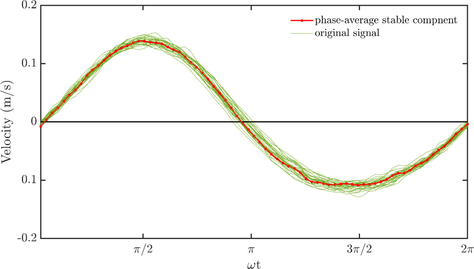
Figure 3 The demonstration of phase-average method: decomposition of the velocity into stable components and turbulence components.

Subsequently, the horizontal and vertical turbulence intensities (σ_u and σ_w) can be calculated as follows:

$\begin{array}{ll}{\sigma }_u=\sqrt{\overline{{u\prime }^2,}}& (3)\end{array}$

$\begin{array}{ll}{\sigma }_w=\sqrt{\overline{{w\prime }^2.}}& (4)\end{array}$

As mentioned earlier, the vertical distributions of SSC were measured during a steady state according to the OBS signal. By applying the time-averaged (over the wave period) advection-diffusion equation during a steady state, the sediment mixing coefficient (ϵ_s) can be derived based on measured SSCs and settling velocity  ω_s (Ogston and Sternberg, 2002; van Rijn, 2007):

$\begin{array}{ll}C\left(z\right){\omega }_s+{ϵ}_s\frac{dC}{dz}=\mathrm{0,}& (5)\end{array}$

where  C (z) is the time-averaged concentration at height z above the sediment bed, ϵ_s is the sediment mixing coefficient and ω_s is the settling velocity of the suspended sediment particles, which can be determined from the following formulations (van Rijn, 1990; te Slaa et al., 2013):

$\begin{array}{ll}{\omega }_s=\{\begin{array}{c}\frac{\left(s-1\right)g{d}^2}{18v} \text{for}1<d\le 100\mu m\\ \frac{10v}{d}\left[{\left(1+\frac{0.01\left(s-1\right)g{d}^3}{v^2}\right)}^{0.5}-1\right] \text{for}100<d\le 1000\mu m\\ 1.1{\left[\left(s-1\right)gd\right]}^{0.5} \text{for}d\ge 1000\mu m\end{array}& (6)\end{array}$

in which d is the median size of the suspended sediment particles and can be measured by sampling method, s is the sediment relative density (= 2.65), and v is the kinematic viscosity coefficient. It is well known that the settling velocity can be affected by various factors, such as particle shape, flocculation, and the sediment concentration itself. The percentages of fine-grained particles (i.e., grain size smaller than 8 µm) of both sediment S1 and S2 are 0.8%-4% (Figure 2). van Ledden et al. (2004) suggested that the sediment mixture behaves as non-cohesive when the clay content (grain size smaller than 2 µm) is smaller than 5%-10%. Thus, both sediment S1 and S2 are considered non-cohesive. Meanwhile, previous settling experiments also showed no flocculation for suspended silt (te Slaa et al., 2013; te Slaa et al., 2015; Xu et al., 2022). Furthermore, Yao et al. (2022a) discovered that silty sediment with grain size larger than 8 µm does not flocculate in freshwater (0‰ of salinity), which is consistent with our experimental phenomena. Therefore, flocculation was not considered. The hindered settling is an important process in case of high SSC to estimate the ω_s . The larger the SSCs, the smaller the settling velocity of the particle. Therefore, the hindered settling effect is considered by multiplying a coefficient Φ_hs=(1−0.65c_t/c_gel)⁵ to ω_s . The c_gel is the volume concentration of the immobile sediment bed, c_gel=(D₅₀/d_sand)c_gel,s , c_gel,s is the dry bulk density and c_t is the total volume concentration.

3. Results

3.1. Vertical distributions of SSC

Figure 4 shows the vertical profiles of SSC for S1 and S2, respectively. By comparison, the SSC profiles of both S1 and S2 are of the same magnitude as the previous studies under wave-only conditions (Su et al., 2015; Yao et al., 2015), so the rationality and repeatability of our experiments can be proved.

FIGURE 4

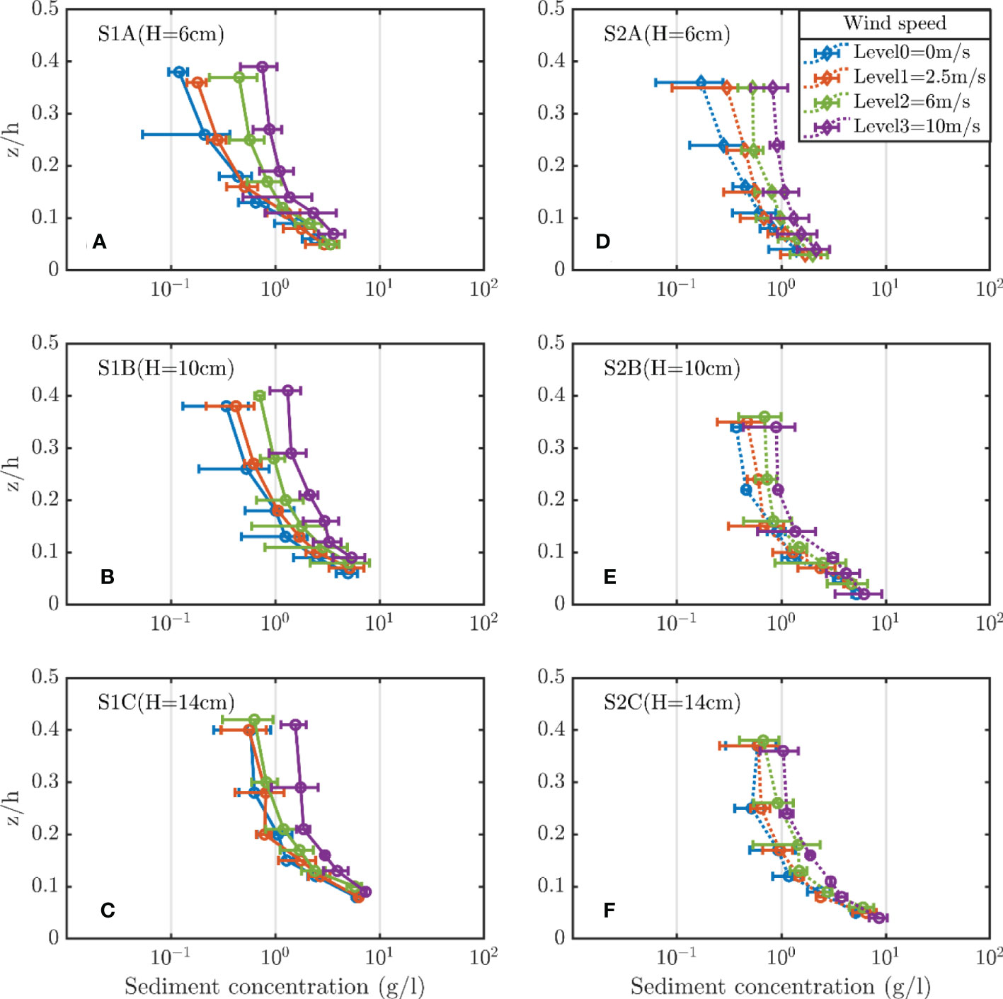
Figure 4 Vertical concentration profiles of S1 (solid lines, A–C) and S2 (dashed lines, D–F). Lines of different colors represent waves combined with the wind of various strengths. The capital letters in the upper left of each graph represent the sediment type and the experimental case. Bars are ensemble standard deviations.

Under paddle wave-only conditions (blue lines in each subplot), larger wave height results in higher SSC of S1. As the wave height increase, the increment of SSC in the middle layers of the water column is more remarkable than in the lower layers, making the SSC profiles more homogeneous in vertical. Compared to S1, the SSC profiles over S2 show the same pattern. However, for the vertical-averaged SSC, c_t2 are smaller than c_t1 under the same wave height (Table 2), indicating that fine sediment is easier to suspend in the water column to increase the water SSC.

TABLE 2

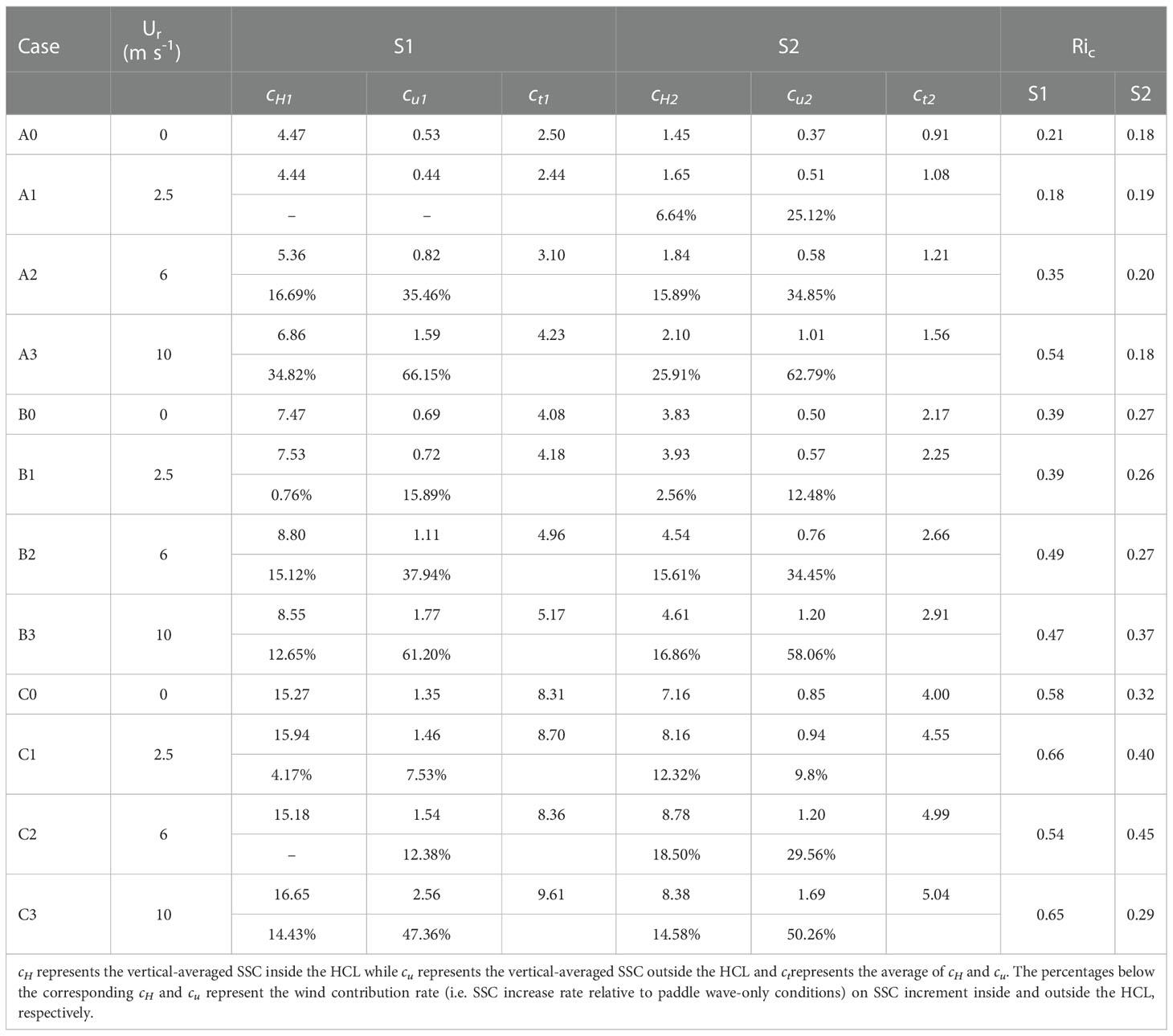
Table 2 The vertical-averaged SSC and bulk Richardson number (Ri_c) of the HCL for S1 and S2 under various experimental conditions, respectively.

When the wind is superposed with paddle waves, the SSCs of S1 increase by different degrees, and the SSC distribution patterns of the three cases with different wind speeds are similar. Taking case S1B as an example (i.e., paddle wave height of 10 cm, Figure 4B), the SSC profile is similar to the wave only condition under relatively small wind (2.5m/s), and then the SSCs increase correspondingly with increasing wind speed, especially in the middle layers. When the wind speed is 6m/s, the SSC increment is 41.42% compare to the wave-only condition in the lowest measuring layer while it keeps increasing upward and reaches 275% in the middle layer (z/h=0.37). As the wind grows up to 10m/s, the SSC of each layer enhances significantly. In the lowest measuring layer, the increment is 50.63% followed by a remarkable increase of over ten times to 525% in the middle layer. One similar phenomenon with the wave-only condition is that the SSC profiles, for all the cases, become homogenizing gradually with the increased wind speed, which is more evident above z/h=0.2. This reveals that under different wind conditions, the SSCs in the middle layers are promoted significantly compared to those in the lowest measuring layers.

The variations of SSC for S2 are generally similar to those of S1 when additional wind is imposed. With increased wind speed, the SSC magnitude of S2 at each elevation increases correspondingly with a more homogeneous profile shape than S1. Besides, the c_t2 is smaller than the c_t1 under the same conditions (wave and wind). This is consistent with the phenomenon of wave-only conditions since the S2 is composed of fewer fine grains than S1.

3.2. Vertical distributions of turbulence intensities

The horizontal and vertical turbulence intensities, σ_u and σ_w, at different elevations above the sediment bed were averaged over wave periods and displayed in Figures 5, 6, respectively. We also compared the results of SFE under similar wind and wave conditions. Note that, different from the fixed bed level in the SFE, the mean bed levels in this study are different for each case due to variations in bedforms.

FIGURE 5

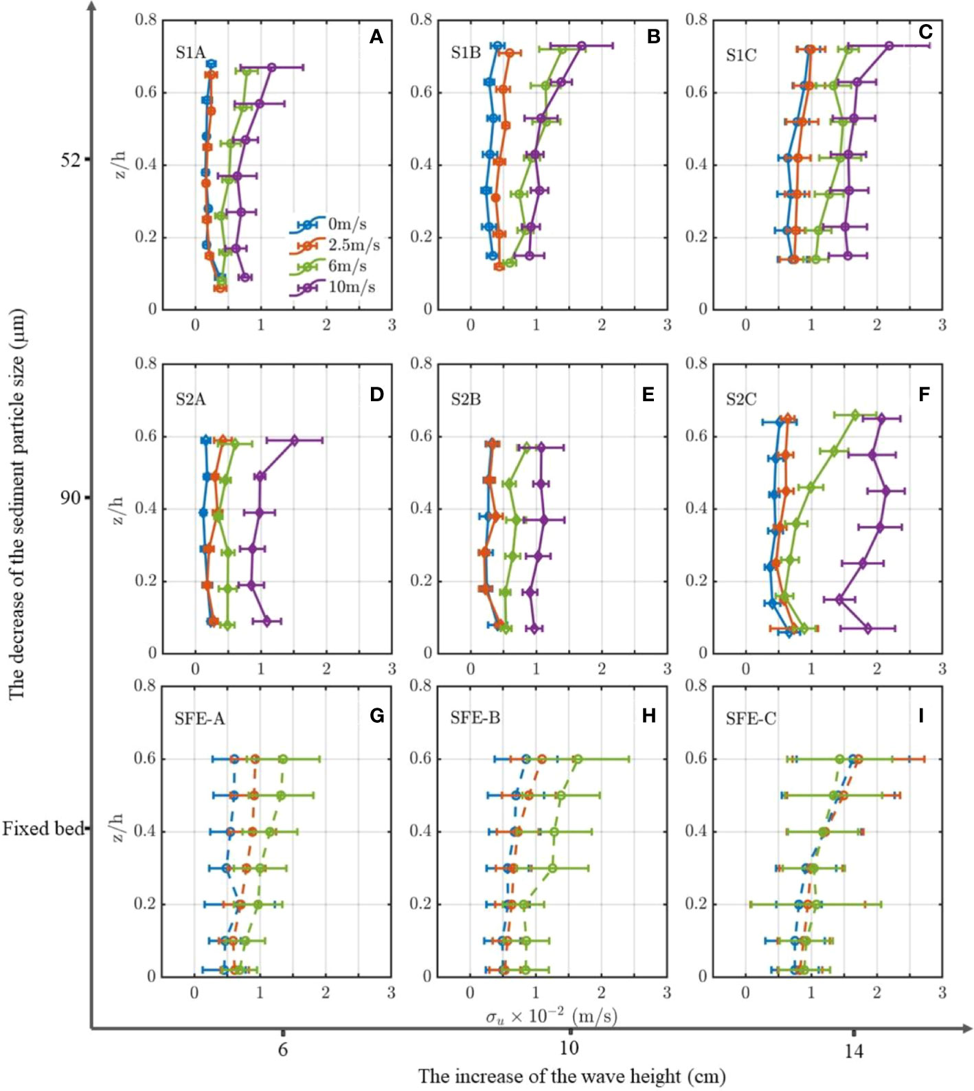
Figure 5 Time-averaged σ_u of S1 (A–C), S2(D–E) and 2017-SFE (G–I). Lines of different colors represent waves combined with the wind of various strengths. The capital letters in the upper left of each graph represent the sediment type and the experimental case. Bars are ensemble standard deviations.

FIGURE 6

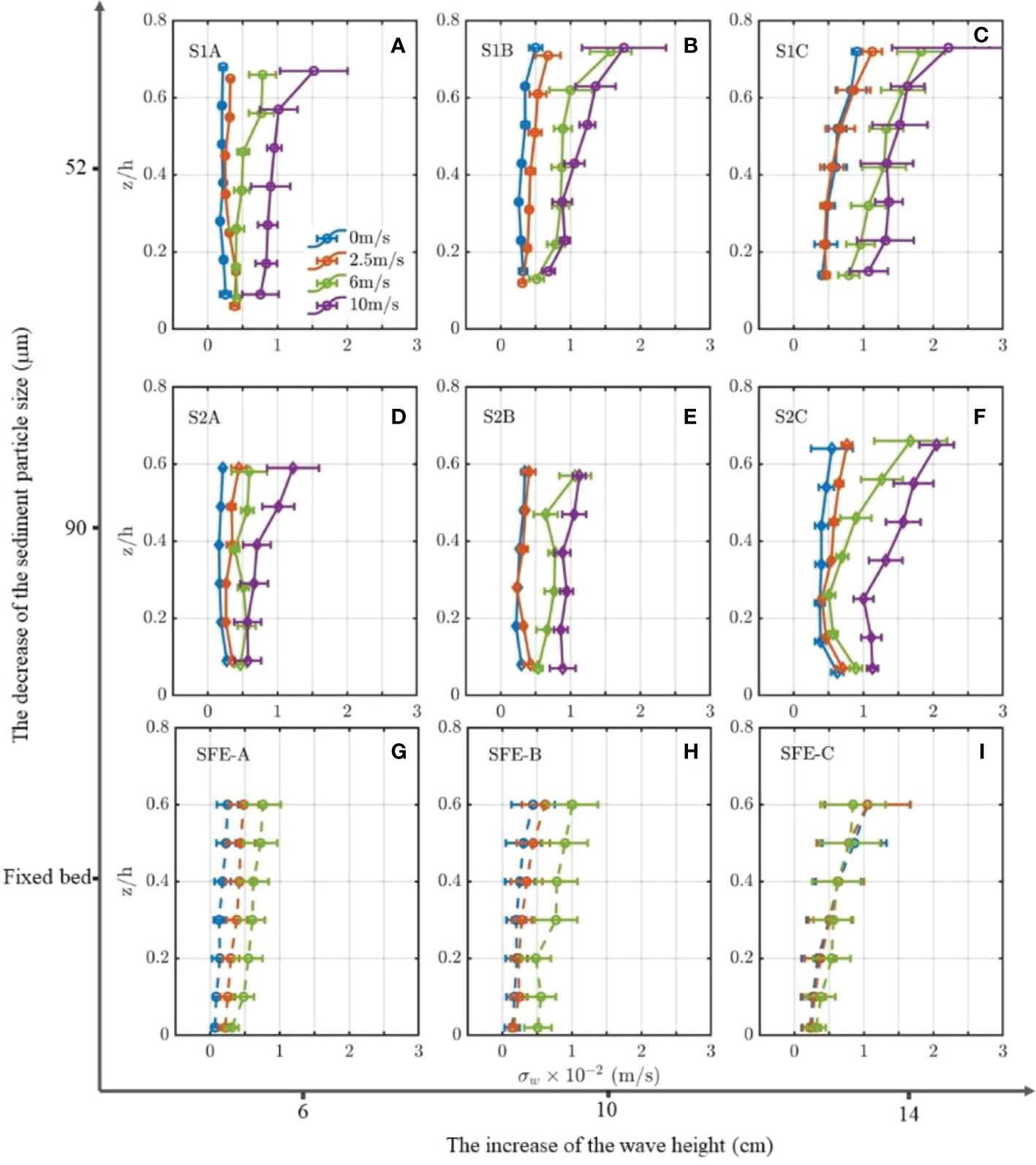
Figure 6 Time-averaged σ_w of S1 (A–C), S2(D, E) and 2017-SFE (G–I). Lines of different colors represent waves combined with the wind of various strengths. The capital letters in the upper left of each graph represent the sediment type and the experimental case. Bars are ensemble standard deviations.

Under paddle wave-only conditions (blue lines in each subplot of Figure 5), compared to the corresponding conditions of SFE (Figures 5G–I), the σ_u profiles over the sediment bed of S1 (Figures 5A–C) are more homogeneous in vertical without evident gradient as the results of SFE. The magnitudes of σ_u over the sediment bed of S1 in each case are smaller than those of SFE, especially in the upper layers (z/h=0.2). The reduction of σ_u in upper layers is because part of the turbulence energy is consumed by maintaining sediment suspension. Meanwhile, the σ_u is reinforced near the bed to a certain degree due to the development of the wave ripples. Compared to S1, the σ_u profiles of S2 exhibit a similar pattern with a relatively small magnitude (Table 1). This reveals that coarse sediment suspensions consume more energy than fine ones.

When the wind is added, the σ_u of both S1 and S2 increase with the wind speed proportionally (Figure 5). For S1, when the wind speed is 2.5m/s, the σ_u profile of each case is similar to the wave-only condition with slightly larger magnitudes. However, as the wind becomes more substantial (i.e., 6m/s, 10m/s), the profiles of σ_u exhibit vertical gradient shapes, which is consistent with the pattern of SFE. For example, the σ_u are reinforced significantly in case S1C2 (i.e., 6m/s wind) and are nearly twice as large on average as those in S1C1 (i.e., 2.5m/s wind) in each elevation (Table 1 and Figure 5). The increase rate of corresponding vertical-averaged value exceeds 58%. The increment declines with the elevation downward, indicating that the wind-induced energy transfers downward into the water with attenuation. This phenomenon is in line with that of SFE. Besides, it can be found that the value of σ_u is smaller than the corresponding result of SFE under the same wave and wind conditions (Table 1). For S2, compared to S1, there are mainly two differences. First, the σ_u profiles are basically homogeneous along the water depth and show no significant gradient shape in each case, even under stronger winds (6m/s and 10m/s) except S2C2. Second, the σ_u values are not as large as S1, as shown by v-σ_u in Table 1. Furthermore, the σ_u enhancement of S2 is more promoted in lowest measuring layers than in S1.

Regarding vertical turbulence intensities, the σ_w of S1 increases with wave height under paddle wave-only conditions (Figures 6A–C). As the wind is superimposed with the paddle wave, the σ_w increases correspondingly with the wind speed by different degrees, similar to the variation pattern of σ_u. For example, the σ_w, in S1C3 (i.e., 10 m/s wind) at each elevation is twice larger on average than the results of relatively minor wind (S1C0 and S1C1). The corresponding increase rates of vertical averaged values are 138.7% and 131.3%, respectively. Compared to the σ_w of SFE, the σ_w profile of S1 only display a gradient shape under stronger wind (6m/s and 10m/s) and more considerable wave height (10cm and 14cm) in case S1B and S1C. In contrast, the profiles are homogenous in vertical under wave-only and 2.5m/s wind conditions. It is worth noting that the σ_w values of S1A are lower than those of SFE but they overtake the SFE as the wave and wind intensify (case S1B and S1C, Figures 6B, C and Table 1). This is different from that of σ_u, which is always smaller than SFE.

In the cases of S2A and S2B, the σ_w profiles are relatively homogeneous in vertical, whereas noticeable gradient shapes only appear in S2C2 and S2C3 (Figures 6D–F). Overall, the σ_w profiles of S2 are consistent with S1, but the magnitudes are smaller. Meanwhile, the σ_w magnitude in S2A is smaller than that of SFE while it is larger in S2B and S2C. This is consistent with the phenomenon of S1 in general. Moreover, the enhancement of σ_w in the lowest measuring layers due to bed forms of S2 is more promoted than S1.

4. Discussions

4.1. How sediment suspensions respond to different wind conditions

In natural systems, the wind blows across the water surface constantly, propagating energy into the water column and affecting water motions and suspended sediments in various ways. Water waves are the most notorious form of wind-induced movement, and the wave-induced turbulence inside the wave boundary layer is the primary driven source of sediment suspension. Similarly, the vertical profile of SSC exhibits a gradient shape that decreases from the wave boundary layer toward the water surface (Figure 4). Figure 7 shows the relationship between depth-averaged SSCs and bed shear stress under different experimental conditions. Under the same paddle wave conditions, the near bed orbital velocity is similar with different wind speeds (Table 1), and the resulting bed shear stress is also similar. This implies that surface wind blowing can hardly influence bed shear stress. For both sediment S1 and S2, the SSC is increased with bed shear stress. The fine-grained sediment (i.e., sediment S1) leads to larger SSCs than the coarser one (i.e., sediment S2) when the bed shear stress is the same.

FIGURE 7

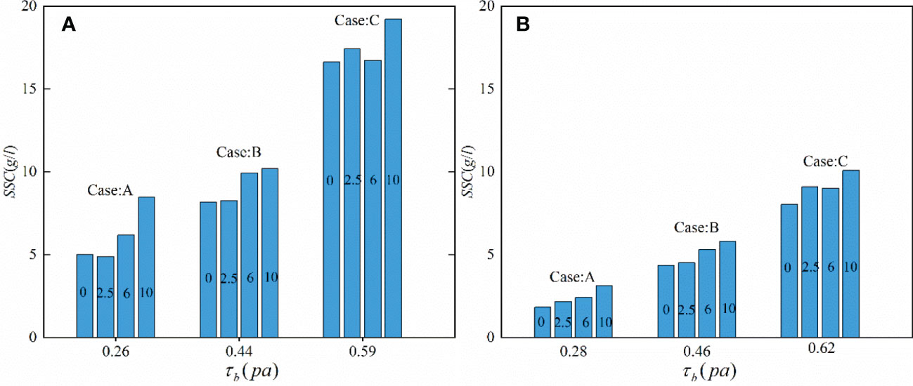
Figure 7 The relationship between bed shear stress and SSC for sediment S1 (A) and S2 (B). The column represents the SSC, and the number in each column denotes the wind speed (unit: m/s) in the corresponding case.

Figure 7 indicates that under the same bed shear stress, there is an increased trend of SSC with increased wind speed, implying an enhanced effect of wind on SSCs. In combination with Figures 4–6 and Table 2, the wind can enhance turbulence intensities in addition to wave-supported sediment suspension, leading to an increase of SSCs mainly in the upper water column (i.e., outside wave boundary layers). This implies that under wind and wave conditions, orbital wave motion controls the suspended sediment dynamics inside the wave boundary layers. In contrast, wind can interfere with sediment mixing processes in terms of wind-induced turbulence outside the wave boundary layers. The results indicate that the stronger the winds, the more homogeneous the SSC profile and the higher the SSC magnitude that can be developed.

To explore to what extent the SSCs respond to the winds, we first define relative wind strength, i.e., the ratio of wind speed to the maximum near-bed velocity, and then investigate the relationship between the increment (δ) of vertical-averaged SSCs and the relative wind strength in Figure 8. A linear curve, fitted with data from different combinations of winds and waves, depicts a positive correlation between the two terms. This further confirms that the wind can enlarge the SSCs but the enhancement depends on the relative strength between the local winds and offshore waves (e.g., swells during rough weather).

FIGURE 8

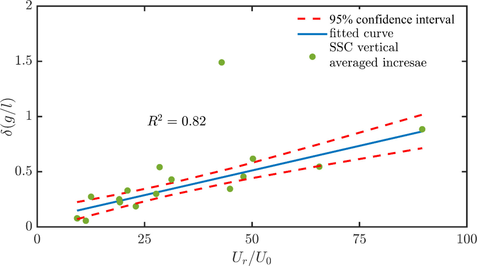
Figure 8 The SSC increments of various experimental cases verse the relative wind strength.

Furthermore, we separate the depth-averaged SSC into two parts, inside and outside the HCL, respectively, and calculate the wind contribution rate on the increment of SSC (Table 2). The SSC for both inside and outside the HCL increases proportionally with the increase of wind speed but in different magnitudes. The SSC increase rates inside the HCL are generally below 20%, whereas they can be as large as 66.15% (S1A3) outside the HCL. This indicates that the wind mainly promotes the SSC outside the HCL while the wave-induced turbulence maintains the SSC inside the HCL.

4.2. Mechanisms underlying the SSC enhancement by winds

During rough weather, offshore wind-generated waves (e.g., swells) propagate into shallow waters, touch the seabed, and entrain bed sediment into suspension. Wave-induced turbulence is a significant force that maintains sediment suspension balancing with the settling process. Thus, when the local wind is superimposed with offshore waves, the increase of SSC (see Figure 4) can be attributed to either the enhancement of turbulence intensities or the reduction of settling velocity. On the one hand, when the wind is introduced, wind-induced turbulence can be transferred into the water column, coupling with wave-induced turbulence, enhancing both horizontal and vertical turbulence intensities (σ_u and σ_w) (Figures 5, 6). Our previous clean-water experiment (SFE, Table 1) also suggested that the σ_w is more sensitive to the wind than σ_u. On the other hand, finer particles with smaller settling velocities can lead to larger SSC and are more sensitive to wind than coarser ones (Figure 4 and Table 2).

With surface blowing wind, the horizontal intensity (σ_u) would be increased, contributing to sediment suspension variations by influencing the lateral dispersion process. The σ_u of both S1 and S2 is smaller than that of SFE (sediment-free experiment) and only shows a gradient under relatively stronger winds (i.e., 6m/s and 10m/s). This indicates that a part of the increased horizontal turbulence energy is consumed by maintaining the lateral dispersion of suspended sediments. Thus, under the same condition, coarser sediments S2 tend to consume more energy than the finer sediments S1, as shown by v-σ_u of S1 and S2 (Table 1).

Regarding the vertical intensity (σ_w), the enhancement of σ_w by winds directly alters the vertical diffusion processes of suspended sediments. The larger σ_w, the larger the SSC with a more homogenous profile shape (Figure 6 and Table 1). In contrast to σ_u, the σ_w of both S1 and S2 is larger than that of SFE, indicating a controversial way wind affects sediment diffusion in horizontal and vertical directions. This can be explained by developing the high concentration layer (HCL) over sand-silt mixtures, where the turbulent motion can be significantly constrained (Trowbridge and Kineke, 1994; Kineke et al., 1996; Yao et al., 2015). To characterize the stratification effect inside HCL, the bulk Richardson number (Ri_c) is chosen (Wright et al., 2001):

$\begin{array}{ll}R{i}_c=s\text{'}c{\text{'}}_{ave}g{\delta }_{HCL}/{{\left(U_{\delta }/3\right)}^2}^{,}& (7)\end{array}$

where s′=s−1 is the relative excess density; c'_ave is the averaged HCL concentration in volume; g is the gravity acceleration;  δ_HCL is the HCL thickness and U_δ is the maximum orbital velocity near bed. The Ri_c of steady stratified flow is approximately 0.25 but varies with grain sizes. In this study, the thickness of HCL was defined as twice the thickness of the wave boundary layer according to Yao et al. (2015). The relative water depth of each measuring elevation is different in each experiment case. In some cases, there were only one or two SSC measurement points inside HCL. Therefore, the data extrapolation method was applied toward reference height to ensure the vertically averaged SSC calculation. The Ri_c of HCL (see Table 2) exceeds 0.25 except for A0 and A1 for S1 and A0-A3 for S2, confirming the existence of stable HCLs under the present experimental conditions. Hence, wind-induced turbulence can hardly penetrate HCL due to the stratification effect but can exert more effects on turbulence intensities outside HCL.

Figure 9 depicts a conceptual diagram showing how wind influence SSCs by turbulence intensification outside the HCL. Under wave-only conditions (i.e., offshore swells), a steady HCL can be formed over sand-silt mixtures. When local winds overlay with swells, both σ_u and σ_w are intensified, which is only effective outside HCL. Subsequently, increasing σ_w by wind-induced turbulence can lift more suspended sediment to a higher elevation, increasing vertical suspended sediment flux and resulting in a more homogenous SSC profile. Meanwhile, the enlargement of SSC in the upper water column further increases the burden of lateral diffusion processes, reducing σ_u. Finally, after a period of feedback adjustment, a new steady state can be achieved.

FIGURE 9

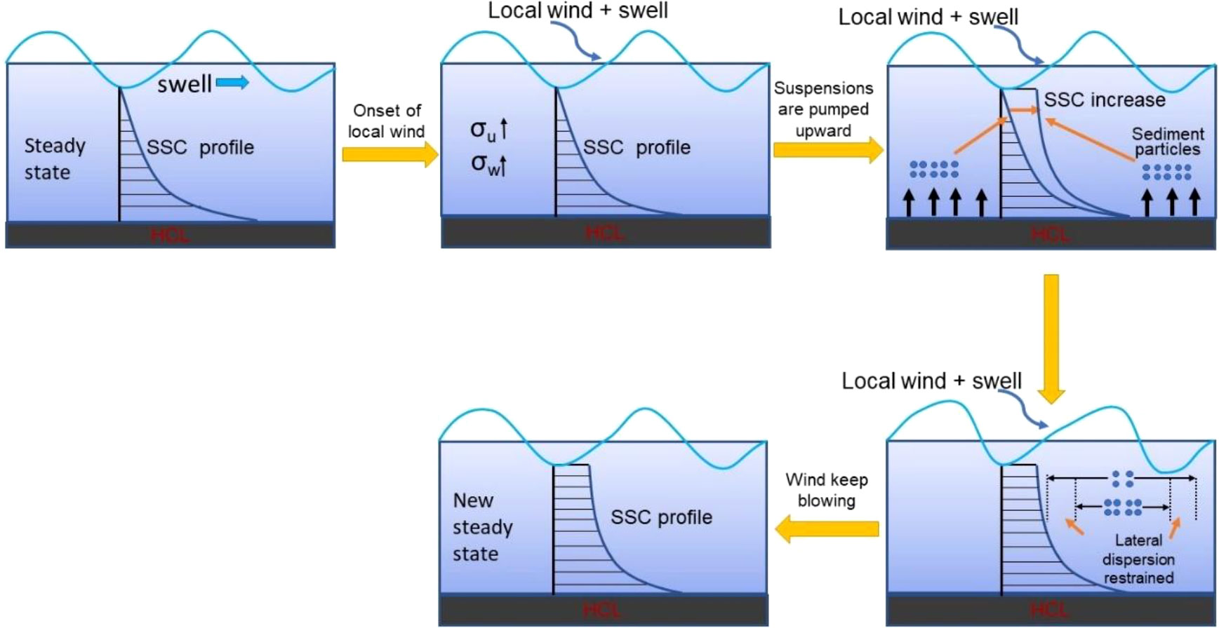
Figure 9 The concept diagram on mechanisms of wind effects on SSCs outside the HCL.

4.3. Estimation of vertical mixing coefficient during rough weather

The vertical mixing coefficient, ϵ_s, is one of the most important parameters that describe the vertical diffusion of suspended sediment and the calculation of SSCs in numerical models. In order to interpret the wind effect on vertical distributions of SSC and the mixing process of suspended silty particles, the ϵ_s have been deduced from the measured SSCs according to Eq. (5). Meanwhile, the calculated ϵ_s are then compared with results based on the widely applied wave-related mixing coefficients proposed by Van Rijn et al. (1993):

$\begin{array}{ll}{ϵ}_{s,w}\left(z\right)=\{\begin{array}{c}{ϵ}_{s,w,bed}={\alpha }_b{U}_{\delta }{\delta }_s \text{for} z\le {\delta }_s\\ {ϵ}_{s,w,max}=\frac{0.0035hH}{T} \text{for}z\ge 0.5h\\ {ϵ}_{s,w,bed}+\left({ϵ}_{s,w,max}-{ϵ}_{s,w,bed}\right)\frac{z-{\delta }_s}{0.5h-{\delta }_s}\text{for }{\delta }_s <z < 0.5h\end{array}& (8)\end{array}$

where α_b=0.0018D_* , D_*= D₅₀[(s−1)]g/ν²]^1/3 , U_δ is the peak near-bed peak orbital velocity; δ_s is the thickness of the sediment mixing layer, and z is the vertical elevation above the sediment bed.

Figure 10 illustrates comparisons of vertical distributions of ϵ_s from measured SSCs (by Eq.(5) and from Eq. (8). Note that the calculation of the SSC gradient starts from the lowest measurement point, so only five points of the mixing coefficient are displayed. Under wave-only conditions, the ϵ_s of S1, for the three cases, display roughly the same pattern. Below z/h=0.1, the ϵ_s remains relatively stable, with a slight increase above z/h=0.1. As the wind was introduced, the ϵ_s varied correspondingly with the wind speed. In S1B, for example, the ϵ_s increase slightly when the wind speed is 2.5m/s; however, when the wind speed increases to 10m/s, the ϵ_s of z/h=0.1 enhances significantly. Concerning S2, the ϵ_s display a similar pattern under both wave-only and wave with wind conditions. One difference is that the ϵ_s of S2 is larger than that of S1 under the same dynamic conditions.

FIGURE 10

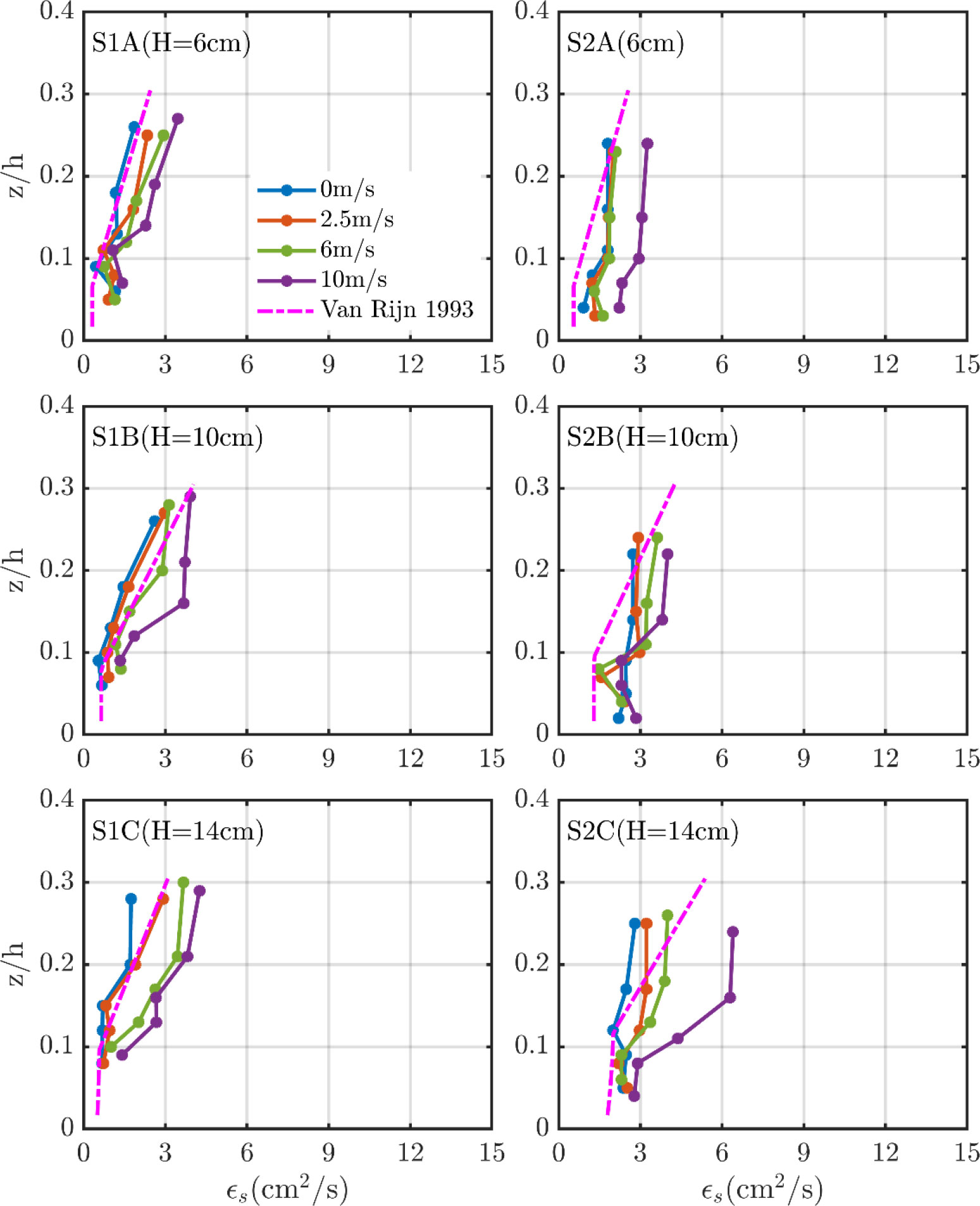
Figure 10 The sediment mixing coefficient, ϵ_s of each case, and the pink dotted dash lines are the theoretical modeled results of Van Rijn et al. (1993).

The ϵ_s under wave only and small wind conditions (2.5m/s) show better agreement with Van Rijn et al. (1993). However, in relatively stronger wind conditions (6m/s and 10m/s), the model may underestimate the ϵ_s, especially for the elevations above z/h=0.1. Considering van Rijn’s model is derived from the fine sand (D_{50 =} 200µm) under wave-only conditions, it can be drawn that the model can be applied for wave-only and minor wind conditions in shallow waters, while for rough weather, the mixing coefficients need to be expanded to avoid the underestimation of SSCs. Deriving a quantitative estimation model of the ϵ_s under wind and wave conditions would be a future research direction to improve the performance of numerical modeling.

5. Conclusions

The present study investigated the influence of local wind on sediment suspension over silt-dominated mixtures using a wind-wave flume experiment. Different combinations of paddle waves (representing swells) with wind speeds (representing local wind waves) have been conducted to explore the wind-induced effect on the SSCs and turbulence structures in addition to the wave. The following conclusions can be summarized:

During rough weather, the swell wave is the primary driver maintaining the high concentration layer near the bottom over silt-dominated mixtures, while local wind can promote more suspensions in the water, especially in the upper water column. The stronger the wind, the higher the SSCs develop. Furthermore, the fine sediment S1 is more sensitive to wind than coarse grains.

The vertical turbulence intensity σ_w, which is enhanced in the upper water column than in the lowest measuring layer, is the main reason for the increased SSCs. The wind contribution to SSC increment can be over 65% outside the HCL. By contrast, the wind contribution rates inside the HCL all remain less than 20%, indicating the main driver of the HCL during rough weather is the swell wave-induced turbulence. Meanwhile, the existence of the HCL hampered the further downward transfer of the surface wind-induced turbulence into the HCL.

Further analyses on the vertical mixing coefficient of sediment suspensions also depict an enhancement of mixing processes by local wind, especially in the upper layer. Hence, it is necessary to consider the enhancement of SSCs when predicting sediment suspension during rough weather in fine-grained systems. Future studies may focus on formulating a modified ϵ_s considering wind effects to increase the modeling accuracy of suspended sediment transport in rough weather.

Data availability statement

The raw data supporting the conclusions of this article will be made available by the authors, without undue reservation.

Author contributions

Conceptualization, YC and PY; methodology, PY and JP; formal analysis, JP, MS, and QZ; data curation, PY and CX; writing—original draft preparation; YC, JP, and PY. Writing—review & editing, MS and ZZ; visualization, JP, ZQ, and QZ. All authors have read and agreed to the published version of the manuscript.

Funding

This work was funded jointly by the National Natural Science Foundation of China (Grant No. 51979076, 51709288, 51909038, 51620105005) and the Open Research Fund of State Key Laboratory of Estuarine and Coastal Research (Grant No. SKLEC-KF202006). PY and MS gratefully acknowledge the Jiangsu Provincial Innovative and Entrepreneurial Doctor Program.

Conflict of interest

The authors declare that the research was conducted in the absence of any commercial or financial relationships that could be construed as a potential conflict of interest.

Publisher’s note

All claims expressed in this article are solely those of the authors and do not necessarily represent those of their affiliated organizations, or those of the publisher, the editors and the reviewers. Any product that may be evaluated in this article, or claim that may be made by its manufacturer, is not guaranteed or endorsed by the publisher.

Supplementary material

The Supplementary Material for this article can be found online at: https://www.frontiersin.org/articles/10.3389/fmars.2022.1036381/full#supplementary-material

References

Aagaard T., Hughes M. G. (2010). Breaker turbulence and sediment suspension in the surf zone. Mar. Geol. 271, 250–259. doi: 10.1016/j.margeo.2010.02.019

CrossRef Full Text | Google Scholar

Alsina J. M., van der Zanden J., Cáceres I., Ribberink J. S. (2018). The influence of wave groups and wave-swash interactions on sediment transport and bed evolution in the swash zone. Coast. Eng. 140, 23–42. doi: 10.1016/j.coastaleng.2018.06.005

CrossRef Full Text | Google Scholar

Bailard J. A. (1981). An energetics total load sediment transport model for a plane sloping beach. J. Geophys. Res. 86, 10938. doi: 10.1029/JC086iC11p10938

CrossRef Full Text | Google Scholar

Bailey M. C., Hamilton D. P. (1997). Wind induced sediment resuspension: A lake-wide model. Ecol. Model. 99, 217–228. doi: 10.1016/S0304-3800(97)01955-8

CrossRef Full Text | Google Scholar

Benilov A., Kouznetsov O. A., Panin G. N. (1974). On the analysis of wind wave-induced disturbances in the atmospheric turbulent surface layer. Bound.-Layer Meteorol. 6, 269–285. doi: 10.1007/BF00232489

CrossRef Full Text | Google Scholar

Booth J. G., Miller R. L., McKee B. A., Leathers R. A. (2000). Wind-induced bottom sediment resuspension in a microtidal coastal environment. Cont. Shelf Res. 20, 785–806. doi: 10.1016/S0278-4343(00)00002-9

CrossRef Full Text | Google Scholar

Cheng Z., Mitsuyasu H. (1992). Laboratory studies on the surface drift current induced by wind and swell. J. Fluid Mech. 243, 247. doi: 10.1017/S0022112092002714

CrossRef Full Text | Google Scholar

Cheung T. K., Street R. L. (1988). The turbulent layer in the water at an air–water interface. J. Fluid Mech. 194, 133. doi: 10.1017/S0022112088002927

CrossRef Full Text | Google Scholar

Cloern J. E. (1987). Turbidity as a control on phytoplankton biomass and productivity in estuaries. Cont. Shelf Res. 7, 1367–1381. doi: 10.1016/0278-4343(87)90042-2

CrossRef Full Text | Google Scholar

Davies A. G., Thorne P. D. (2016). On the suspension of graded sediment by waves above ripples: Inferences of convective and diffusive processes. Cont. Shelf Res. 112, 46–67. doi: 10.1016/j.csr.2015.10.006

CrossRef Full Text | Google Scholar

Gong Z., Jin C., Zhang C., Zhou Z., Zhang Q., Li H. (2017). Temporal and spatial morphological variations along a cross-shore intertidal profile, jiangsu, China. Cont. Shelf Res. 144, 1–9. doi: 10.1016/j.csr.2017.06.009

CrossRef Full Text | Google Scholar

Green M. O., Coco G. (2014). Review of wave-driven sediment resuspension and transport in estuaries. Rev. Geophys. 52, 77–117. doi: 10.1002/2013RG000437

CrossRef Full Text | Google Scholar

Hassan W. N., Ribberink J. S. (2005). Transport processes of uniform and mixed sands in oscillatory sheet flow. Coast. Eng. 52, 745–770. doi: 10.1016/j.coastaleng.2005.06.002

CrossRef Full Text | Google Scholar

Hooshmand A., Horner-Devine A. R., Lamb M. P. (2015). Structure of turbulence and sediment stratification in wave-supported mud layers. J. Geophys. Res. Oceans 120, 2430–2448. doi: 10.1002/2014JC010231

CrossRef Full Text | Google Scholar

Hu Z., Yao P., Wal van der D., Bouma T. J. (2017). Patterns and drivers of daily bed-level dynamics on two tidal flats with contrasting wave exposure. Sci. Rep. 7, 7088. doi: 10.1038/s41598-017-07515-y

PubMed Abstract | CrossRef Full Text | Google Scholar

Jacobs W., Le Hir P., Van Kesteren W., Cann P. (2011). “Erosion threshold of sand–mud mixtures,” in Cont. Shelf Res., Proceedings of the 9th International Conference on Nearshore and Estuarine Cohesive Sediment Transport Processes, Netherlands: Elsevier. Vol. 31. S14–S25. doi: 10.1016/j.csr.2010.05.012

CrossRef Full Text | Google Scholar

Kassem H., Thompson C. E. L., Amos C. L., Townend I. H. (2015). Wave-induced coherent turbulence structures and sediment resuspension in the nearshore of a prototype-scale sandy barrier beach. Cont. Shelf Res. 109, 78–94. doi: 10.1016/j.csr.2015.09.007

CrossRef Full Text | Google Scholar

Kineke G. C., Sternberg R. W., Trowbridge J. H., Geyer W. R. (1996). Fluid-mud processes on the Amazon continental shelf. Cont. Shelf Res. 16, 667–696. doi: 10.1016/0278-4343(95)00050-X

CrossRef Full Text | Google Scholar

Kobayashi N., Payo A., Schmied L. (2008). Cross-shore suspended sand and bed load transport on beaches. J. Geophys. Res. Oceans 113, C07001. doi: 10.1029/2007JC004203

CrossRef Full Text | Google Scholar

Lamb M. P. (2004). Turbulent structure of high-density suspensions formed under waves. J. Geophys. Res. 109, C12026. doi: 10.1029/2004JC002355

CrossRef Full Text | Google Scholar

Liu J. H., Yang S. L., Zhu Q., Zhang J. (2014). Controls on suspended sediment concentration profiles in the shallow and turbid Yangtze estuary. Cont. Shelf Res. 90, 96–108. doi: 10.1016/j.csr.2014.01.021

CrossRef Full Text | Google Scholar

Maa P.-Y., Mehta A. J. (1987). Mud erosion by waves: A laoratory study. Cont. Shelf Res. 7, 1269–1284. doi: 10.1016/0198-0254(88)92531-9

CrossRef Full Text | Google Scholar

Mansard E. P. D., Funke E. R. (1980). “The measurement of incident and reflected spectra using a least squares method,” Coastal Engineering. 1980 United States: ASCE 154–172.

Google Scholar

Mariotti G., Fagherazzi S. (2013). Wind waves on a mudflat: The influence of fetch and depth on bed shear stresses. Cont. Shelf Res. 60, S99–S110. doi: 10.1016/j.csr.2012.03.001

CrossRef Full Text | Google Scholar

Mitchener H., Torfs H. (1996). Erosion of mud/sand mixtures. Coast. Eng. 29, 1–25. doi: 10.1016/S0378-3839(96)00002-6

CrossRef Full Text | Google Scholar

Mitsuyasu H., Yoshida Y. (2005). Air-Sea interactions under the existence of opposing swell. J. Oceanogr. 61, 141–154. doi: 10.1007/s10872-005-0027-1

CrossRef Full Text | Google Scholar

Ogston A. S., Sternberg R. W. (2002). Effect of wave breaking on sediment eddy diffusivity, suspended-sediment and longshore sediment flux profiles in the surf zone. Cont. Shelf Res. 22, 633–655. doi: 10.1016/S0278-4343(01)00033-4

CrossRef Full Text | Google Scholar

O’Hara Murray R. B., Hodgson D. M., Thorne P. D. (2012). “Wave groups and sediment resuspension processes over evolving sandy bedforms,” in Cont. shelf res Netherlands: Elsevier, vol. 46. , 16–30. The application of acoustics to sediment transport processes. doi: 10.1016/j.csr.2012.02.011

CrossRef Full Text | Google Scholar

Olfateh M., Ware P., Callaghan D. P., Nielsen P., Baldock T. E. (2017). Momentum transfer under laboratory wind waves. Coast. Eng. 121, 255–264. doi: 10.1016/j.coastaleng.2016.09.001

CrossRef Full Text | Google Scholar

Pang W., Dai Z., Ma B., Wang J., Huang H., Li S. (2020). Linkage between turbulent kinetic energy, waves and suspended sediment concentrations in the nearshore zone. Mar. Geol. 425, 106190. doi: 10.1016/j.margeo.2020.106190

CrossRef Full Text | Google Scholar

Pu J., Chen Y., Su M., Mei J., Yang X., Yu Z., et al. (2022). Residual sediment transport in the fine-grained jiangsu coast under changing climate: The role of wind-driven currents. Water 14, 3113. doi: 10.3390/w14193113

CrossRef Full Text | Google Scholar

Qiao F., Yuan Y., Deng J., Dai D., Song Z. (2016). Wave–turbulence interaction-induced vertical mixing and its effects in ocean and climate models. Philos. Trans. R. Soc Math. Phys. Eng. Sci. 374, 20150201. doi: 10.1098/rsta.2015.0201

CrossRef Full Text | Google Scholar

Sanford L. P. (2008). Modeling a dynamically varying mixed sediment bed with erosion, deposition, bioturbation, consolidation, and armoring. Comput. Geosci. 34, 1263–1283. doi: 10.1016/j.cageo.2008.02.011. Predictive Modeling in Sediment Transport and Stratigraphy.

CrossRef Full Text | Google Scholar

Soulsby R. L., Humphery J. D. (1990). Field Observations of Wave-Current Interaction at the Sea Bed. In: Tørum A., Gudmestad O. T. (eds) Water Wave Kinematics. NATO ASI Series, vol 178. Dordrecht: Springer. doi: 10.1007/978-94-009-0531-3_25

CrossRef Full Text | Google Scholar

Su M., Yao P., Wang Z. B., Chen Y. P., Zhang C. K., Stive M. J. F. (2015). Laboratory studies on the response of fine sediment to wind. Proceedings of 36th IAHR World Congress (the Hague, The Netherlands: Taylor & Francis), 1–9.

Google Scholar

Su M., Yao P., Wang Z., Zhang C., Chen Y., Stive M. J. F. (2016). Conversion of electro-optical signals to sediment concentration in a silt–sand suspension environment. Coast. Eng. 114, 284–294. doi: 10.1016/j.coastaleng.2016.04.014

CrossRef Full Text | Google Scholar

Sun H. Q., Wang Y. X., Peng J. P. (2002). Hilbert Transform applied to separation of waves. China Ocean Eng. 16, 239–248.

Google Scholar

Tao Z. J., Chu A., Chen Y. P., Lu S. Q., Wang B. (2020). Wind effect on the saltwater intrusion in the Yangtze estuary. J. Coast. Res. 105 (SI), 42–46. doi: 10.2112/JCR-SI105-009.1

CrossRef Full Text | Google Scholar

te Slaa S., He Q., van Maren D. S., Winterwerp J. C. (2013). Sedimentation processes in silt-rich sediment systems. Ocean Dynamics 63, 399–421. doi: 10.1007/s10236-013-0600-x

CrossRef Full Text | Google Scholar

te Slaa S., van Maren D., He Q., Winterwerp J. (2015). Hindered settling of silt. J. Hydraul. Eng. 141 (9), 04015020. doi: 10.1061/(ASCE)HY.1943-7900.0001038

CrossRef Full Text | Google Scholar

Thais L., Magnaudet J. (1996). Turbulent structure beneath surface gravity waves sheared by the wind. J. Fluid Mech. 328, 313–344. doi: 10.1017/S0022112096008749

CrossRef Full Text | Google Scholar

Thorne P. D., Williams J. J., Davies A. G. (2002). Suspended sediments under waves measured in a large-scale flume facility. J. Geophys. Res. 107, 3178. doi: 10.1029/2001JC000988

CrossRef Full Text | Google Scholar

Trowbridge J. H., Kineke G. C. (1994). Structure and dynamics of fluid muds on the Amazon continental shelf. J. Geophys. Res. 99, 865. doi: 10.1029/93JC02860

CrossRef Full Text | Google Scholar

van Ledden M., van Kesteren W. G. M., Winterwerp J. C. (2004). A conceptual framework for the erosion behaviour of sand–mud mixtures. Continental Shelf Res. 24, 1–11. doi: 10.1016/j.csr.2003.09.002

CrossRef Full Text | Google Scholar

van Ledden M., Wang Z. B., Winterwerp H., de Vriend H. (2006). Modelling sand–mud morphodynamics in the friesche zeegat. Ocean Dyn. 56, 248–265. doi: 10.1007/s10236-005-0055-9

CrossRef Full Text | Google Scholar

van Rijn (1989). Handbook sediment transport by currents and waves (2nd ed.). Delft Hydraulics Laboratory.

Google Scholar

van Rijn L. C. (2007). Unified view of sediment transport by currents and waves. II: Suspended Transport. J. Hydraul. Eng. 133, 668–689. doi: 10.1061/(ASCE)0733-9429(2007)133:6(668

CrossRef Full Text | Google Scholar

van Rijn L. C., Kroon A. (1992). “Sediment transport by currents and waves, in: Coastal engineering 1992,” in Presented at the 23rd International Conference on Coastal Engineering, American Society of Civil Engineers. United States, ASCE. 2613–2628. doi: 10.1061/9780872629332.199

CrossRef Full Text | Google Scholar

van Rijn L. C., Louisse C. J. (1987). “The effect of waves on cohesive bed surface. Proceedings on Coastal and Port Engineering; Netherlands, A.A. Balkema.

Google Scholar

van Rijn L. C., Nieuwjaar M. W. C., van der Kaay T., Nap E., van Kampen A. (1993). Transport of fine sands by currents and waves. J. Waterw. Port Coast. Ocean Eng. 119, 123–143. doi: 10.1061/(ASCE)0733-950X(1993)119:2(123

CrossRef Full Text | Google Scholar

Waeles B., Hir P. L., Lesueur P. (2008). “Chapter 32 a 3D morphodynamic process-based modelling of a mixed sand/mud coastal environment: The seine estuary, France,” in Proceedings in marine science, sediment and ecohydraulics. Eds. Kusuda T., Yamanishi H., Spearman J., Gailani J. Z. (Netherlands: Elsevier), 477–498. doi: 10.1016/S1568-2692(08)80034-4

CrossRef Full Text | Google Scholar

Wright L. D., Friedrichs C. T., Kim S. C., Scully M. E. (2001). Effects of ambient currents and waves on gravity-driven sediment transport on continental shelves. Mar. Geol. 175, 25–45. doi: 10.1016/S0025-3227(01)00140-2

CrossRef Full Text | Google Scholar

Wu D., Hua Z. (2014). The effect of vegetation on sediment resuspension and phosphorus release under hydrodynamic disturbance in shallow lakes. Ecol. Eng. 69, 55–62. doi: 10.1016/j.ecoleng.2014.03.059

CrossRef Full Text | Google Scholar

Xu B., Gong Z., Zhang Q., Zhang C., Zhao K. (2018). Non-equilibrium suspended sediment transport on the intertidal flats of jiangsu coast, China. sJ. Coast. Res. 85, 251–255. doi: 10.2112/SI85-051.1

CrossRef Full Text | Google Scholar

Xu C., Odum B., Chen Y., Yao P. (2022). Evaluation of the role of silt content on the flocculation behavior of clay-silt mixtures. Water Resour. Res. 58, e2021WR030964. doi: 10.1029/2021WR030964

CrossRef Full Text | Google Scholar

Yao P., Sun W., Guo Q., Su M. (2022a). Experimental study on the effect of sediment composition and water salinity on settling processes of quartz silt in still water. J. Sediment Res. 47 (5), 15–22.

Google Scholar

Yao P., Su M., Wang Z., van Rijn L. C., Stive M. J. F., Xu C., et al. (2022b). Erosion behavior of sand-silt mixtures: Revisiting the erosion threshold. Water Resour. Res. 58, e2021WR031788. doi: 10.1029/2021WR031788

CrossRef Full Text | Google Scholar

Yao P., Su M., Wang Z., van Rijn L. C., Zhang C., Chen Y., et al. (2015). Experiment inspired numerical modeling of sediment concentration over sand–silt mixtures. Coast. Eng. 105, 75–89. doi: 10.1016/j.coastaleng.2015.07.008

CrossRef Full Text | Google Scholar

Zhao C. J. (2003). Study on Power Sand Movement Laws in Coastal Dynamic Condition. PhD Thesis, Tianjin University, China. (in Chinese with English (abstract)

Google Scholar

Zhu Q., van Prooijen B. C., Wang Z. B., Ma Y. X., Yang S. L. (2016). Bed shear stress estimation on an open intertidal flat using in situ measurements. Estuar. Coast. Shelf Sci. 182, 190–201. doi: 10.1016/j.ecss.2016.08.028

CrossRef Full Text | Google Scholar

Zuo L., Roelvink D., Lu Y., Dong G. (2021). Process-based suspended sediment carrying capacity of silt-sand sediment in wave conditions. Int. J. Sediment Res. 37 (2), 229–237. doi: 10.1016/j.ijsrc.2021.09.007

CrossRef Full Text | Google Scholar

Zuo L., Roelvink D., Lu Y., Li S. (2017). On incipient motion of silt-sand under combined action of waves and currents. Appl. Ocean Res. 69, 116–125. doi: 10.1016/j.apor.2017.10.005

CrossRef Full Text | Google Scholar