Importance of the choice of heat flux parameterization in regional air–sea coupled simulations: Case studies of marine heatwaves induced by atmospheric heatwaves in 1994 and 2018

This study investigated the marine heat wave events (MHWs) that occurred near the Korean Peninsula during the summer of 1994 and 2018, using a regional air–sea coupled model. We analyzed the fifth-generation reanalysis data, ERA5, published by the European Centre for Medium-Range Weather Forecasts for both events. We found that the North Pacific High and Tibetan High were stronger than usual and were associated with warm and moist air intrusion from the subtropical regions. Air-sea interactions play an important role in the development of MHWs. Warm and moist air combined with low-level inversion and a subsequent sinking motion induced the downward latent heat flux (LHF) toward the relatively colder sea surface, resulting in increased sea surface temperatures (SSTs). To quantify the contribution of the downward LHF and evaluate the importance of the relevant physical parameters of the MHWs, we set up two coupled model experiments, namely, CPL_down and CPL_nodown. Results show that the CPL_down experiment captured the downward LHF well in both events. The model also successfully captured the observed inversion near the surface. The cold SST bias tended to be reduced as the low-level clouds decreased in the area where the downward LHF occurred. In our simulation, permitting downward LHF improved the MHW reproducibility. Therefore, we suggest that the increased downward LHF is favorable for simulating MHWs, and surface physical parameterization must be carefully performed.

Introduction

Marine heatwave (MHW) conditions occur when the sea surface temperature (SST) exceeds a threshold for several days or more. Holbrook et al (2016) suggested that the SST threshold leading to an MHW is defined as the 90th percentile of SST measurements based on a 30-year historical baseline period. It is necessary to carefully monitor MHWs because they cause severe socio-economic damage and induce complex marine disasters (Holbrook et al, 2016).

MHWs occur worldwide owing to the warming of the oceans. However, the northwest Pacific region, including the Korean Peninsula, shows increased MHW occurrences (Holbrook et al., 2016; Han and Lee, 2020). For example, Lindsey and Dahlman (2021) found a significant increasing trend in ocean heat content for the 0–700 m layer around the Korean Peninsula and the Atlantic Ocean. Lee et al. (2020) also observed that MHW days over the East Asian marginal seas (EAMS) increased by approximately two days in 10 years.

Many attempts have been made to predict or reproduce MHWs using numerical simulation (Kim et al., 2020; Cho et al., 2022); however, such attempts are faced with several difficulties. For example, cold SST biases are common in air–sea coupled models. For example, Kim et al. (2020) confirmed a cold SST bias over the entire northwest Pacific region while reproducing MHWs. Furthermore, Cho et al. (2022) found that the cold SST bias strengthened as the lead time increased in GloSea5. This is caused by the lack of understanding of air–sea interactions. Furthermore, Cho et al. (2022) observed the overestimation of upward latent heat flux (LHF) in the models.

MHWs originate from complex interactions between the ocean and atmosphere (Holbrook et al., 2016). Lee et al. (2020) identified two major modes of MHW over the EAMS using the dates of MHWs and empirical orthogonal functions. The first is an extensive MHW mode that occurs due to the warming of the subtropical northwest Pacific Ocean during El Niño southern oscillation events from early winter. The second mode, which shows a dipole shape in the EAMS, develops abruptly near the Korean Peninsula and occurs primarily due to stagnant anticyclones (Yeo et al., 2019; Lee et al., 2020; Noh et al., 2021). The previous studies have indicated that a strong downward turbulent heat flux (THF), i.e., the sum of sensible heat flux (SHF) and LHF, exists in the Korean Strait when stagnant anticyclones lead to the development of MHWs. Here, notable features of the second mode are similar to the physical mechanism of MHWs caused by the atmospheric forcing listed in Holbrook et al (2016). Specifically, these authors found that, in a persistent high-pressure system, cloud cover and wind speed decrease, and the number of insolation increases. In addition, the mixed-layer depth remains shallow due to suppressed wind speed, moisture flux from the ocean decreases, and the atmosphere is warmed by shortwave radiation. Consequently, an increase in net surface heat flux (i.e., the sum of shortwave radiation, longwave radiation, sensible heat flux, and latent heat flux) results in MHWs.

Among net heat flux terms, LHF is most important in the generation of MHWs from atmospheric heatwaves (AHWs). Generally, LHF is greater than SHF, and, therefore, plays a dominant role along with solar radiation in fluctuations in the net surface energy balance. In addition, the direction of LHF is the same as that of moisture flux, which regulates humidity, meaning that it is closely related to the formation of low-level clouds and net surface shortwave radiation. However, unlike the others, the downward latent heat flux is limited to zero in the default heat flux parameterization of the Weather Research and Forecasting (WRF) model, which is widely used in for coupled air-sea modeling. As downward latent heat flux can occur along with sea fog at the coast (Edson et al., 2007), it requires modification. Therefore, in this study, we simulated MHWs using coupled models that reproduced downward LHF. Furthermore, events caused by stagnant anticyclones were selected from previous studies, and the sensitivity of the numerical models in the parametrization of heat flux was assessed to better understand its role in modulating the development of MHWs from AHWs.

Data and methods

Data

We used the optimum interpolation daily SST (OISST) data from 1982–2020 to select the MHW cases (Reynolds et al., 2002), and monthly ERA5 reanalysis (Hersbach et al., 2020) anomaly data from 1979 to 2020 were obtained. In climate data analysis, the trend is one of the most important amounts. To compare two events of MHWs in 1994 and 2018, the trend is necessary to be removed from the data. In the present study, we simply identified the linear trends for 1982-2020 and 1979–2020 using linear regression and eliminated them from the OISST and ERA5 data, respectively. Moreover, atmospheric variables (e.g., SHF and LHF) in the modern-era retrospective analysis for research and application (MERRA-2; Gelaro et al., 2017) and OISST were utilized to validate the simulation results. We also employed the hybrid coordinate ocean model (HYCOM; Chassignet et al., 2003) for the model experiments.

Case description

Previous studies on the MHWs around the Korean Peninsula show some common characteristics (Yeo et al., 2019; Lee et al., 2020; Noh et al., 2021). For example, high atmospheric pressure and downward THF were observed throughout the Yellow Sea and the East Sea. The downward THF implies the inversion of temperature and humidity at the sea surface, which is an uncommon phenomenon globally (Cho et al., 2000; Brunke et al., 2015). Particularly, the downward LHF denotes that the humidity at the sea surface is assumed to be saturated due to the air–sea interaction. However, during early summer, due to AHWs, insufficient heating over the ocean around the Korean Peninsula produces favorable conditions for inversion. AHWs during early summer are related to the North Pacific High (Wang et al., 2000). Here, we focus the air–sea interactions occurring in association with the AHW events in 1994 and 2018 (Lee et al., 2020), which are the two highest-ranked AHW events in the Korean Peninsula region that were accompanied by MHWs.

The MHWs in 1994 and 2018 were strengthened by the effects of AHWs rather than warm currents from the subtropical Pacific Ocean. Due to the oceanic forcing, the MHWs developed steadily over several months (Holbrook et al., 2016; Lee et al., 2020). However, comparing the two MHW cases with the climatological SSTs (Figure 1), abrupt increases in the SST anomalies around the Korean Peninsula occurred. Figure 2 shows the geopotential height anomalies at 500 hPa, and moist static energy (MSE) at 850 hPa, in East Asia for July 1994 and 2018. The developing strong anticyclones over the East Asian region are favorable for transporting warm and humid air from the subtropical region to the Korean Peninsula (Figures 2A, B). Here, AHWs can be classified into two types: extreme (hot and dry) and oppressive (hot and humid) (Ford and Schoof, 2017). Anomalously high MSE implies the occurrence of oppressive AHWs and the influx of warmer and more humid air (Figures 2C, D). Figure 3 presents the detrended temperature and specific humidity differences between air (2 m above the ocean) and sea surface. Oppressive AHWs increased the air–sea temperature difference by 0.8 K, reaching the maximum in 1994 and 2018 around the Korean Peninsula. Furthermore, the air-side specific humidity was 1.5 g/kg higher than the saturated sea surface humidity, which provided favorable conditions for downward LHF and caused MHWs around the Korean Peninsula by suppressing heat release from the oceans.

FIGURE 1

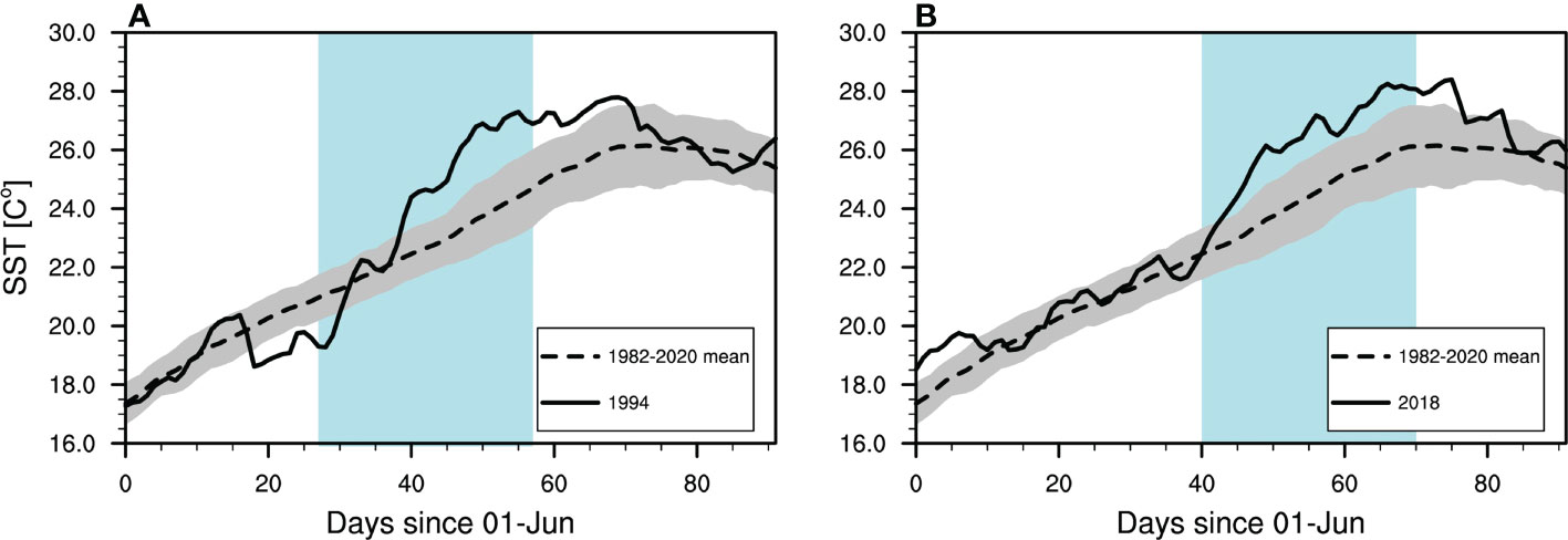
Figure 1 Time-series plots of daily mean sea surface temperature (solid), climatological mean (dashed), and interannual variability with one standard deviation (gray shading) around the Korean Peninsula (33.5–37.5° N, 124.0–131.0° E) for 1994 (A) and 2018 (B), respectively. The daily climatological mean and standard deviation is calculated for 1982–2020. Colored areas represent the selected model periods for each case.

FIGURE 2

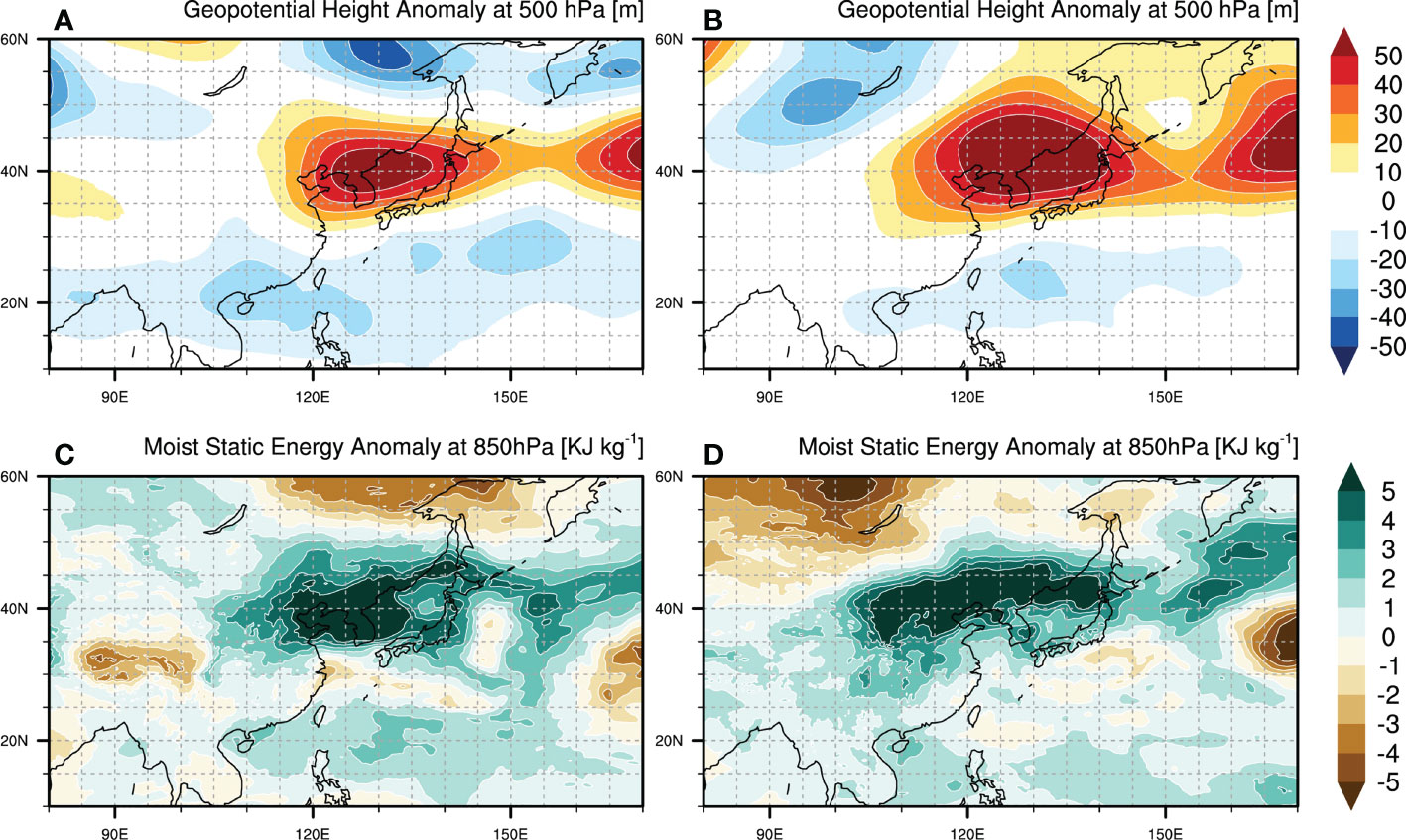
Figure 2 Horizontal distribution of geopotential height anomalies at 500 hPa (A, B); m and moist static-energy anomalies at 850 hPa (C, D); KJ kg⁻¹ in July 1994 (left) and 2018 (right), respectively, in East Asia (10–60° N, 80–170° E).

FIGURE 3

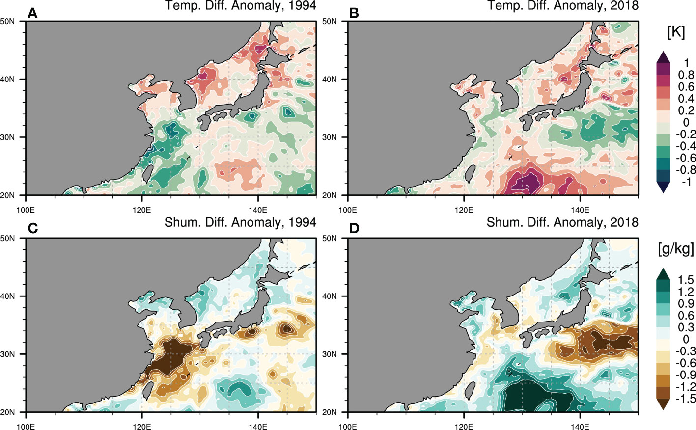
Figure 3 Horizontal distribution of detrended air–sea temperature difference anomalies (A, B); K and specific humidity difference anomalies (C, D); g kg⁻¹ in July 1994 (left) and 2018 (right), respectively, in East Asia (10–60° N, 80–170° E). Shum: specific humidity. All variables are used from ERA5 data.

Model configuration

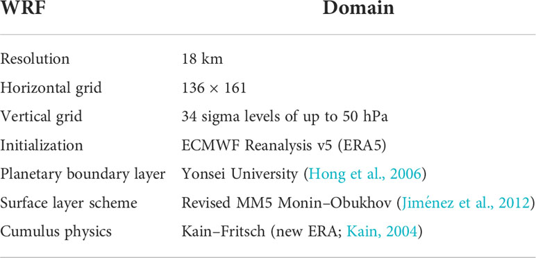
We selected the coupled–ocean–atmosphere–wave–sediment transport (COAWST; Warner et al., 2010) framework as the air–sea coupled model to reproduce the two events of MHWs. We coupled the Regional Ocean Modeling System (ROMS; Shchepetkin and McWilliams, 2005) and the WRF (Skamarock et al., 2019). The COAWST exchanges the variables between ROMS and the WRF using the model coupling toolkit (Larson et al., 2005). The model domain is illustrated in Figure 4. The Revised MM5 Monin–Obukhov scheme (Jiménez et al., 2012), which is designed to limit the downward LHF that may occur during the model integration, was used for the surface layer scheme for the WRF (Table 1). We conducted two experiments (i.e., CPL_down and CPL_nodown) to investigate the effect of the downward LHF on the simulation results. Here, the downward LHF was allowed in the CPL_down but was forced and fixed at zero in the CPL_nodown. The overall experimental design is presented in Figure 5. The initial and open boundary conditions for the ROMS were provided by HYCOM GOFS 3.0: HYCOM + NCODA Global 1/12° Reanalysis (GLBu0.08/reanalysis for 1994) and HYCOM GOFS 3.0: HYCOM + NCODA Global 1/12° Analysis (GLBu0.08/expt_91.2 for 2018). In addition, the initial and boundary condition for the WRF was provided by the ERA5 reanalysis dataset. Based on the OISST data (Figure 1), the initial times for our two experiments were set at June 28 for the 1994 event and July 10 for the 2018 event.

FIGURE 4

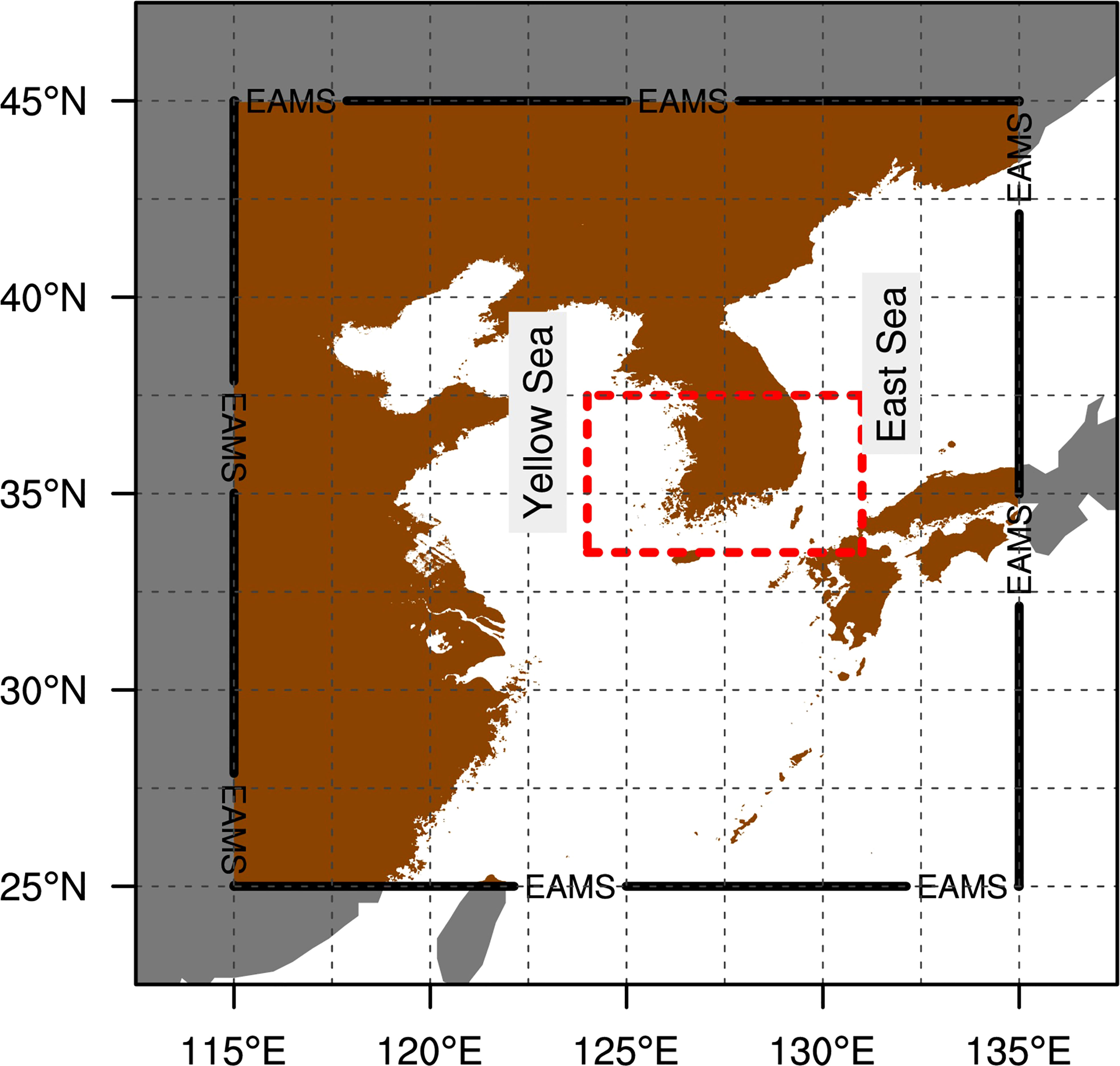
Figure 4 Model domain for the Weather Research and Forecasting (WRF) and Regional Ocean Modeling System (ROMS) models. The East Asia marginal seas (EAMS) and the analysis region are shown with a solid black line and a red dotted line, respectively.

TABLE 1

Table 1 Overview of weather research and forecasting (WRF) configurations used in this study.

FIGURE 5

Figure 5 Schematic representation of the experimental design.

Results

Comparisons with reanalysis data

Each MHW was simulated for 30 days from the onset of the drastic increase in the area-averaged SST anomaly (red box in Figure 4) around the Korean Peninsula. Compared to the reanalysis data, the overall increasing trend in SST was modeled well for the 1994 case (Figure 6A). Compared to the CPL_nodown experiment, the cold SST bias in the CPL_down experiment was reduced from 0.5 K to 1 K.

FIGURE 6

Figure 6 Time series plots of daily area-averaged mean values of sea surface temperature (SST) (A), surface net latent heat flux (LHF) (B), and surface net sensible heat flux (SHF) (C) time series for the reanalysis data (black), CPL_down (red) and CPL_nodown (blue) simulations, and the OISST data (grey in A only) over the analysis region (33.5–37.5° N, 124.0–131.0° E) for the 1994 case.

MERRA2 showed a downward LHF over the ocean for a few days after the initialization period (Figure 6B). The positive values imply an upward direction of movement. In comparison, downward LHF did not occur in the CPL_nodown model, for which no downward LHF was permitted. On the other hand, in the CPL_down model, a minimum LHF of −40 Wm⁻² was simulated. Although this is an overestimate compared to the MERRA2 data, the overall trend in the CPL_down model was close to that of the MERRA2 model. From the 20th day, the upward LHF began to strengthen via sea surface warming. We observed that the overall trend in LHF was overestimated compared to the MERRA2 model. Similarly, SHF was higher in the CPL_down experiment than in CPL_nodown experiment (Figure 6C).

Heat budget analysis

A heat budget analysis for the mixed layer was conducted to investigate the contribution of the four components of the net surface heat flux in the vertical integral of the governing equation for the upper ocean temperature. We used a simple form of the tendency equation for the mixed layer (Eq. 1), for which the decomposition of the budget terms followed Pak et al. (2022):

$\begin{array}{ll}MLTtendency=Q+HADV+OVMIX& (1)\end{array}$

where MLR  tendency s the temporal change in the mixed layer temperature, Q s the net surface heat flux term, the HADV s the horizontal advection term, and OVMIX s the ocean vertical mixing term. We mainly focused on the first budget term of net surface heat flux, which refers to the role of atmospheric forcing in developing MHWs. The Q term is defined as:

$\begin{array}{ll}Q=\frac{Q_{net}}{{\rho }_0{c}_{p}h}& (2)\end{array}$

where Q_net s the net surface heat flux at the air-sea interface, ρ₀ s water density (1,027 kg m^-3), c_p s the specific heat capacity of seawater at constant pressure (4,300 J/kg C), and h s the mixed layer depth. Q_net is composed of net shortwave radiation, net longwave radiation, SHF, and LHF. A positive value of this term indicates that the ocean gains heat from the atmosphere.

Figure 7 depicts the daily time series of the area-averaged mixed layer temperature (MLT) tendency and Q term from the simulation results. During the entire period, the warming of the MLT tendency was almost entirely explained by changes in the Q term. The differences between the two simulation results indicate that the contribution of downward LHF was sensitive to SST warming by shortwave radiation. In the case of the heat fluxes, the differences in the mean contribution of shortwave radiation, longwave radiation, SHF, and LHF during the entire period were +0.05°C/day, +0.01°C/day, +0.004°C/day, and +0.005°C/day, respectively. Thus, the increase in shortwave radiation likely caused SST warming.

FIGURE 7

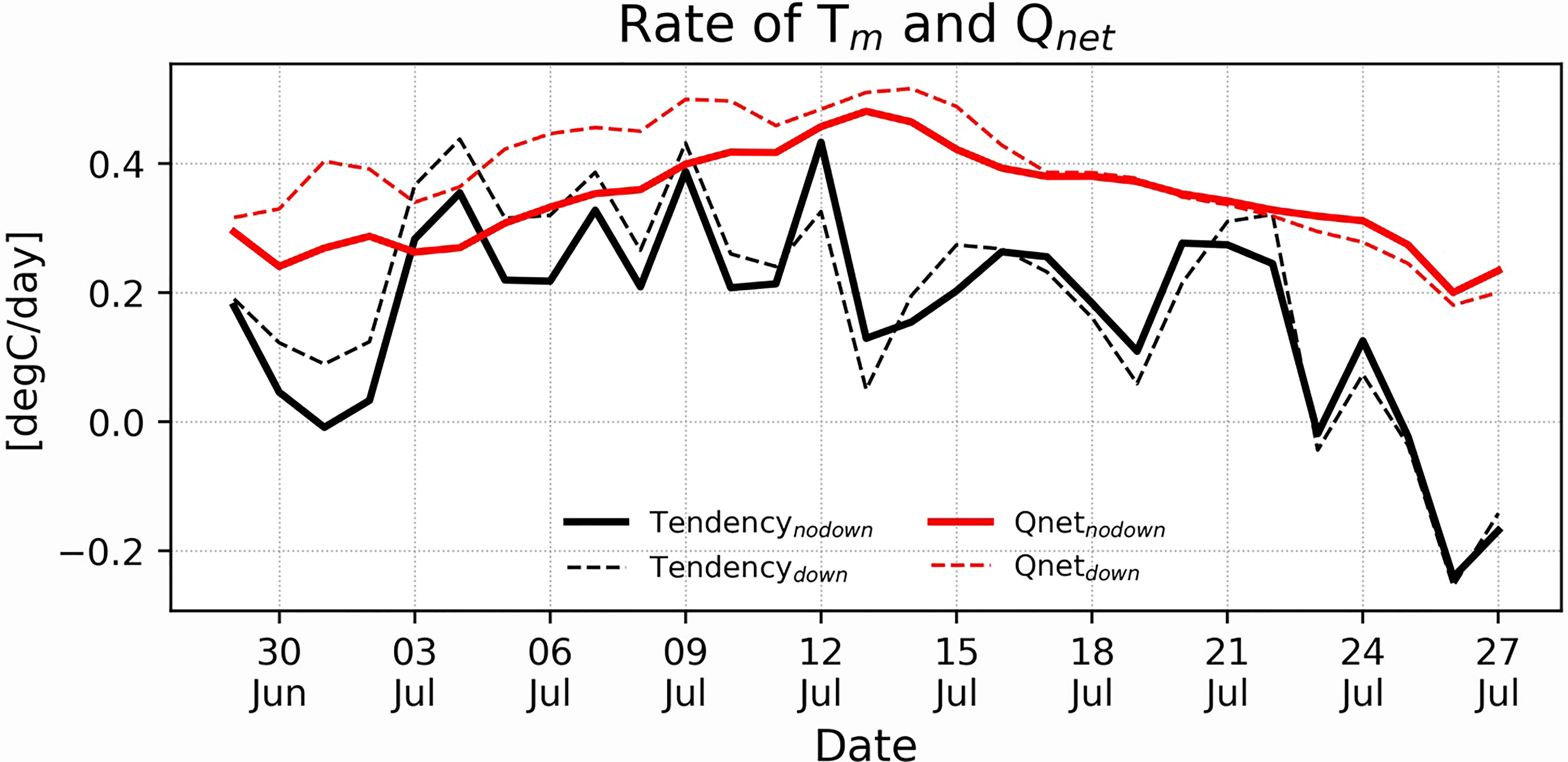
Figure 7 Time-series plots of depth-averaged water temperature (T_m) for the mixed layer (tendency; in black) and the net surface heat flux Q_net (red) for the CPL_nodown (solid) and CPL_down (dashed) simulations over the analysis region (33.5–37.5° N, 124.0–131.0° E). Q_net is the sum of net shortwave radiation, net longwave radiation, sensible heat flux, and latent heat flux. T_m is depth-averaged water temperature up to the mixed layer.

Impacts of downward LHF

The SST heating rates (i.e., the increase in SST per hour) were derived from each simulation to analyze the effect of LHF in resolving the cold SST bias. Figure 8 illustrates the differences in the SST heating rates between the two simulations for the 1994 case during daytime and nighttime. Every 24 hours, a positive and negative phase appears during the daytime and nighttime, respectively. This indicates that solar radiation is a major factor in the increase in SST due to the downward LHF. A high heating rate was observed during the daytime in both the East Sea and Yellow Sea, where warm and humid air is transported from low latitudes along the geopotential height at 925 hPa. In contrast, during the night, when there is no shortwave (SW) radiation, cooling by Planck radiation was strengthened. Notably, the time-averaged heating and cooling effects were comparable; however, heating was dominant during summer because the sunshine duration accounted for 64.8% of the day. Furthermore, stronger heating occurred in the Yellow Sea compared to the East Sea because the anticyclonic wind was dominant over the Korean Strait due to the North Pacific High.

FIGURE 8

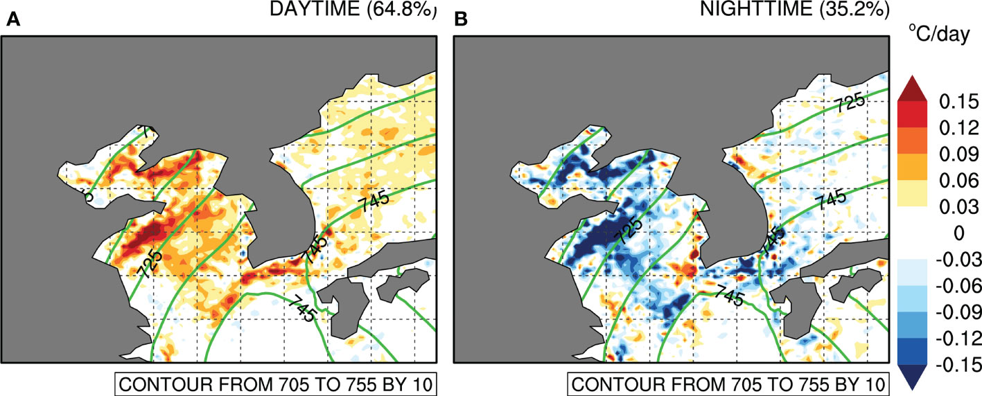
Figure 8 Horizontal distribution of the differences in sea surface temperature (SST) warming rates between the CPL_down and CPL_nodown models for the 1994 case during the daytime (A) and nighttime (B). Positive shading means the heating rate in the CPL_down model was higher than that in the CPL_nodown simulation. Green lines denote the time-averaged geopotential height at 925 hPa.

The relationship between downward LHF and solar radiation at the sea surface can be demonstrated in terms of the low-level cloud fractions (LCFs) for 1,000–700 hPa. Specifically, low-level clouds are thicker and are more efficient at blocking solar radiation than high-level clouds (Watanabe et al., 2018). Koshiro and Shiotani (2014) classified low-level clouds into three categories based on pressure, namely stratocumulus (700–850 hPa), stratus (850–925 hPa), and fog (925 hPa to the surface). Of these three types, sea fog is closely related to downward THF over the ocean. By analyzing the estimated inversion strength, Koshiro and Shiotani (2014) showed that sea fog can dramatically increase when temperature inversion occurs. Furthermore, Edson et al. (2007) observed sea fog and downward LHF at the coast, and confirmed that the removal of inversion due to downward LHF can decrease sea fog occurrence. Thus, downward LHF implies a decrease in evaporation; indeed, in both experiments, sea fog was simulated in areas where downward LHF occurred. However, as presented in Figure 9, showing the time series of the vertical structures of the cloud fractions during the 1994 event, sea fog was partially removed in the CPL_down model relative to the CPL_nodown simulation. Therefore, we compared the LCF and SW reproducibility for each experiment using MERRA-2 reanalysis data. Figure 10 shows the LCF and SW time series at the sea surface for the initial 15 days of the 1994 case. Excluding the early part of the simulation, we observed an overall overestimation of the LCFs, which resulted in less SW reaching the surface, as shown in Figure 10B. Nevertheless, the CPL_down model resolved this overestimation and partially adjusted the underestimation of SW compared to the CPL_nodown model.

FIGURE 9

Figure 9 Time series of the vertical structure of cloud fractions passing through the Yellow Sea (36.5–39.0° N, 124.0° E) for the (A) CPL_nodown and (B) CPL_down simulations for the 1994 case.

FIGURE 10

Figure 10 Area mean values of low-level cloud fractions (LCFs) (A) and the surface net short wave time series (B) for the MERRA-2 data (black) and the CPL_down (red) and CPL_nodown (blue) simulations every 3 h for the 1994 case.

Compared to 1994, the sensitivity of downward LHF was not significant around the Korean Peninsula in the experiment for the 2018 case (Figures S1, S2). Because the higher initial SST distributions for the 2018 case than for the 1994 case (about 5°C at maximum) made it hard to generate humidity inversion. In addition, it is notable that the areas where the sensitivity of downward LHF was significant were determined by the transport of air from the subtropical ocean to the Korean Peninsula coastal seas due to the location and size of the North Pacific High during both events (Figures 8, S3).

Summary and discussion

We reproduced and analyzed MHWs using the WRF and ROMS in the COAWST framework to resolve the cold SST bias during summer around the Korean Peninsula. We verified that the cold SST bias can be resolved by allowing downward LHF using the revised MM5 Monin–Obukhov scheme, which is a common heat flux parameterization method in the WRF model. The AHW events that occurred in 1994 and 2018 are representative cases of oppressive AHWs, where the North Pacific High and the Tibetan High were strongly formed over the East Sea. In July 1994 and 2018, warm and humid air was transported from the subtropical region to the Korean seas and caused a strong temperature and humidity inversion. Downward LHF was occurred in both the reanalysis and CPL_down simulations. In particular, MHWs were better simulated by the CPL_down model, in which downward LHF was permitted. The differences in heating between the two simulation results changed phase every 24 hours and were dominated by SW. Crucially, LCF caused the observed difference in SW between the two experiments, having a marked influence on sea fog. Thus, our CPL_down simulation showed improvements in SW and LCF representation as well as SST because they successfully reproduced reductions in sea fog.

Finally, our study suggests that downward LHF should be considered in the development of air–sea coupled model systems over the ocean. Notably, we only reproduced MHWs associated with AHWs, and some caution is required because there is a possibility of downward LHF occurring in early summer. Thus, the downward LHF around the Korean Peninsula indicates that further flux observations and modeling-based research are needed to quantify the accuracy of heat-flux parameterization.

Data availability statement

The raw data supporting the conclusions of this article will be made available by the authors, without undue reservation.

Author contributions

T-BJ, H-JB, and SY initiated and coordinated the work. T-BJ wrote the manuscript, and H-JB, B-MK, and SY revised it. All authors contributed to the article and approved the submitted version.

Funding

This research was carried out through the R&D project "Development of a Next-Generation Numerical Weather Prediction Model by the Korea Institute of Atmospheric Prediction Systems (KIAPS)", funded by the Korea Meteorological Administration (KMA2020-02212).

Acknowledgments

We acknowledge the critical comments from the reviewers and editors.

Conflict of interest

The authors declare that the research was conducted in the absence of any commercial or financial relationships that could be construed as a potential conflict of interest.

Publisher’s note

All claims expressed in this article are solely those of the authors and do not necessarily represent those of their affiliated organizations, or those of the publisher, the editors and the reviewers. Any product that may be evaluated in this article, or claim that may be made by its manufacturer, is not guaranteed or endorsed by the publisher.

Supplementary material

The Supplementary Material for this article can be found online at: https://www.frontiersin.org/articles/10.3389/fmars.2022.1032930/full#supplementary-material

References

Brunke M. A., Stegall S. T., Zeng X. (2015). A climatology of tropospheric humidity inversions in five reanalyses. Atmos. Res. 153, 165–187. doi: 10.1016/J.ATMOSRES.2014.08.005

CrossRef Full Text | Google Scholar

Chassignet E. P., Smith L. T., Halliwell G. R., Bleck R. (2003). North Atlantic simulations with the hybrid coordinate ocean model (HYCOM): impact of the vertical coordinate choice, reference pressure, and thermobaricity. J. Phys. Oceanogr. 33, 2504–2526. doi: 10.1175/1520-0485(2003)033<2504:NASWTH>2.0.CO;2

CrossRef Full Text | Google Scholar

Cho Y. K., Kim M. O., Kim B. C. (2000). Sea Fog around the Korean peninsula. J. Appl. Meteorol. 39, 2473–2479. doi: 10.1175/1520-0450(2000)039<2473:sfatkp>2.0.co;2

CrossRef Full Text | Google Scholar

Cho A., Song H., Tak Y. J., Yeh S. W., An S. I., Lee S. M., et al. (2022). Atmosphere-driven cold SST biases over the western north pacific in the GloSea5 seasonal forecast system. Clim. Dyn., 59, 1–14. doi: 10.1007/S00382-022-06228-X

CrossRef Full Text | Google Scholar

Edson J., Crawford T., Crescenti J., Farrar T., Frew N., Gerbi G., et al. (2007). The coupled boundary layers and air–sea transfer experiment in low winds. Bull. Am. Meteorol. Soc 88 (3), 341–356. doi: 10.1175/BAMS-88-3-341

CrossRef Full Text | Google Scholar

Ford T. W., Schoof J. T. (2017). Characterizing extreme and oppressive heat waves in Illinois. J. Geophys. Res. Atmos. 122 (2), 682–698. doi: 10.1002/2016JD025721

CrossRef Full Text | Google Scholar

Gelaro R., McCarty W., Su´arez M. J., Todling R., Molod A., Takacs L., et al. (2017). The modern-era retrospective analysis for research and applications, version 2 (MERRA-2). J. Clim. 30 (14), 5419–5454. doi: 10.1175/JCLI-D-16-0758.1

PubMed Abstract | CrossRef Full Text | Google Scholar

Han I. S., Lee J. S. (2020). Change the annual amplitude of Sea surface temperature due to climate change in a recent decade around the Korean peninsula. J. Korean Soc March 26 (3), 233–241. doi: 10.7837/KOSOMES.2020.26.3.233

CrossRef Full Text | Google Scholar

Hersbach H., Bell B., Berrisford P., Hirahara S., Horányi A., Muñoz-Sabater J., et al. (2020). The ERA5 global reanalysis. Q. J. R. Meteor. Soc 146, 1999–2049. doi: 10.1002/qj.3803

CrossRef Full Text | Google Scholar

Holbrook N. J., Hobday A. J., Alexander L. V., Perkins S. E., Smale D. A., Straub S. C., et al. (2016). A hierarchical approach to defining MHWs. Prog. Oceanogr. 141, 227–238. doi: 10.1016/J.POCEAN.2015.12.014

CrossRef Full Text | Google Scholar

Hong S. Y., Noh Y., Dudhia J. (2006). A new vertical diffusion package with an explicit treatment of entrainment processes. Monthly Weather Rev. 134, 2318–2341. doi: 10.1175/mwr3199.1

CrossRef Full Text | Google Scholar

Jiménez P. A., Dudhia J., González-Rouco J. F., Navarro J., Montávez J. P., García-Bustamante E. (2012). A revised scheme for the WRF surface layer formulation. Mon. Weather Rev. 140 (3), 898–918. doi: 10.1175/MWR-D-11-00056.1

CrossRef Full Text | Google Scholar

Kain J. S. (2004). The kain-fritsch convective parameterization: An update. J. Appl. Meteorol 43, 170–181. doi: 10.1175/1520-0450(2004)0432.0.co;2.CO;2

CrossRef Full Text | Google Scholar

Kim E. J., Marzin C., Milton S. F., Boo K. O., Kim Y., Oh J., et al. (2020). Representation of the 2016 Korean heatwave in the unified model global NWP forecasts: The impact of remotely forced model errors and atmosphere-ocean coupling. Atmosphere 11 (12), 1275. doi: 10.3390/ATMOS11121275

CrossRef Full Text | Google Scholar

Koshiro T., Shiotani M. (2014). Relationship between low stratiform cloud amount and estimated inversion strength in the lower troposphere over the global ocean in terms of cloud types. J. Meteorol. Soc Japan 92 (1), 107–120. doi: 10.2151/jmsj.2014-107

CrossRef Full Text | Google Scholar

Larson J., Jacob R., Ong E. (2005). The model coupling toolkit: A new Fortran90 toolkit for building multiphysics parallel coupled models. Int. J. High Perform. Comput. Appl. 19 (3), 277–292. doi: 10.1177/1094342005056115

CrossRef Full Text | Google Scholar

Lee H. D., Min K. H., Bae J. H., Cha D. H. (2020). Characteristics and comparison of 2016 and 2018 heat wave in Korea. Atmosphere 30 (1), 1–15. doi: 10.14191/ATMOS.2020.30.1.001

CrossRef Full Text | Google Scholar

Lee S., Park M. S., Kwon M., Kim Y. H., Park Y. G. (2020). Two major modes of East Asian MHWs. Environ. Res. Lett. 15 (7), 074008. doi: 10.1088/1748-9326/AB8527

CrossRef Full Text | Google Scholar

Lindsey R., Dahlman L. (2021) Climate change: Global temperature. Available at: https://www.climate.gov/news-features/understanding-climate/climate-change-global-temperature (Accessed September 28, 2021).

Google Scholar

Noh E., Kim J., Jun S. Y., Cha D. H., Park M. S., Kim J. H., et al. (2021). The role of the pacific-Japan pattern in extreme heatwaves over Korea and Japan. Geophys. Res. Lett. 48 (18), e2021GL093990. doi: 10.1029/2021GL093990

CrossRef Full Text | Google Scholar

Pak G., Noh J., Park Y. G., Jin H., Park J. H. (2022). Governing factors of the record-breaking marine heatwave over the mid-latitude western north pacific in the summer of 2021. Front. Mar. Sci. 9. doi: 10.3389/fmars.2022.946767

PubMed Abstract | CrossRef Full Text | Google Scholar

Reynolds R. W., Rayner N. A., Smith T. M., Stokes D. C., Wang W. (2002). An improved in situ and satellite SST analysis for climate. J. Clim. 15 (13), 1609–1625. doi: 10.1175/1520-0442(2002)015<1609:AIISAS>2.0.CO;2

CrossRef Full Text | Google Scholar

Shchepetkin A. F., McWilliams J. C. (2005). The regional oceanic modeling system (ROMS): a split-explicit, free-surface, topography-following-coordinate oceanic model. Ocean Model. 9 (4), 347–404. doi: 10.1016/J.OCEMOD.2004.08.002

CrossRef Full Text | Google Scholar

Skamarock W. C., Klemp J. B., Dudhia J. B., Gill D. O., Barker D. M., Duda M. G., et al. (2019). A description of the advanced research WRF model version 4.3 (Boulder, CO, USA: National Center for Atmospheric Research), 145.

Google Scholar

Wang B., Wu R., Fu X. (2000). Pacific–East Asian teleconnection: How does ENSO affect East Asian climate? J. Clim. 13 (9), 1517–1536. doi: 10.1175/1520-0442(2000)013<1517:PEATHD>2.0.CO;2

CrossRef Full Text | Google Scholar

Warner J. C., Armstrong B., He R., Zambon J. B. (2010). Development of a coupled ocean–Atmosphere–Wave–Sediment transport (COAWST) modeling system. Ocean Model. 35 (3), 230–244. doi: 10.1016/J.OCEMOD.2010.07.010

CrossRef Full Text | Google Scholar

Watanabe M., Kamae Y., Shiogama H., DeAngelis A. M., Suzuki K. (2018). Low clouds link equilibrium climate sensitivity to hydrological sensitivity. Nat. Clim. Change 8 (10), 901–906. doi: 10.1038/s41558-018-0272-0

CrossRef Full Text | Google Scholar

Yeo S. R., Yeh S. W., Lee W. S. (2019). Two types of heat wave in Korea associated with atmospheric circulation pattern. J. Geophys. Res. Atmos. 124 (14), 7498–7511. doi: 10.1029/2018JD030170

CrossRef Full Text | Google Scholar