Overlapping-calibration of wide-swath altimeter baseline errors using two satellites formation flying design

1 Introduction

The future wide-swath altimetry missions of the Surface Water and Ocean Topography (SWOT) (Fu and Ubelmann, 2014; Morrow et al., 2019) and “Guanlan” (Chen et al., 2019) will provide two-dimensional measurements of ocean surface topography (Dufau et al., 2016; Bonaduce et al., 2018). They are expected to increase the resolvable scale of global ocean to 10-30 km (Chelton et al., 2019). To achieve such oceanography objectives, high-precision sea surface height (SSH) observation is required (Archer et al., 2020). However, multi-source errors of wide-swath altimetry, including random noise (RN), baseline roll and length errors, dry and wet troposphere delay, and sea state bias (Ren et al., 2020), will directly limit the precision of the retrieved SSH data. As a result, one of the most critical studies on the wide-swath altimetry mission is how to reduce the SSH errors (Chen et al., 2021), and for each error source, specific reduction methods should be developed according to the corresponding error model. On this basis, this study focuses on the research of SSH errors associated with baselines, involving height error associated with the both baseline roll (HEBR) and baseline length (HEBL).

The HEBR and HEBL are stemming from imperfect knowledge about the true information of the baseline roll and length. Due to mechanical perturbations and thermal effects, the baseline may be angularly deformed and change in the length in orbit (Dibarboure et al., 2012). Taking “Guanlan” mission as an example (Chen et al., 2019), the effective swath in the cross-track direction is between 15 km to 100 km. Based on the HEBR and HEBL calculation model in (Peral and Esteban-Fernandez, 2018), 0.1 mm baseline length error would bring about 8.4 cm range error on the outer edges of the swath. Generally, a roll error of only 1/3,600 deg (1arcsec) will result in a height error of 48 cm on the outer edge position of 100 km. That is to say, if the HEBR is required to limit to 1 cm at the far end of the swath, the roll error of the baseline needs to be smaller than 20masec. Nevertheless, it is really too difficult to achieve such accuracy of baseline roll measurement for “Guanlan” mission. According to the research results of (Dibarboure et al., 2012), the HEBR and HEBL are not white noise in the along-track direction. Moreover, both errors cannot be separable from the SSH signal in the frequency domain. If the roll measurement accuracy of “Guanlan” can only reach ~1 arcsec, the mean baseline roll error is not only very large (~26.4 cm), but also varies in the along-track direction. In such case, as many fine-scale oceanic signals would not be detected, it is difficult to achieve oceanography objectives (Gonzalez et al., 2010; Gomez-Navarro et al., 2020). Therefore, even though the measurement accuracies of the baseline roll and length are insufficient, it is indeed necessary and vital to find a reliable method of reducing the HEBR and HEBL along all observation swaths.

Previous researches (Gaultier et al., 2016; Fujii et al., 2019; Di et al., 2021; King and Martin, 2021; Benkiran et al., 2022) have employed observing system simulation experiments (OSSEs) to assess the performance of wide-swath altimetry. Furthermore, based on OSSEs, numerous studies (Dibarboure et al., 2012; Dibarboure and Ubelmann, 2014) have attempted to explore the methods of reducing the SSH observation errors due to baseline errors (SSH_Error_Baseline) and aimed to minimize oceanic signal leakages caused by errors. Dibarboure et al. (2012) and Dibarboure and Ubelmann (2014) proposed empirical cross-calibration methods, and they also demonstrated the viability of four empirical cross-calibration methods, namely “direct method”, “crossovers method”, “external nadir crossovers method”, and “sub-cycle overlaps method”. To be specific, the “direct method” is based on the SSH estimated value, such as the high-resolution ocean model or low-resolution SSH grid data. Till the present, these reference data cannot accurately reconstruct or characterize sub-mesoscale (15-50 km) oceanic dynamic processes, which indicates that the accuracies of SSH reference data are not enough (Callies and Wu, 2019; Metref et al., 2020). Hence, this method inevitably generates the leakage of SSH signals, whereas the other three methods can only be applied to reduce local errors, and the residual errors are related with the variation of ocean topography during the time interval of two crossovers or overlap passes (Dibarboure and Ubelmann, 2014). Moreover, the ocean topography must be various (Chen et al., 2021). When the interval time of two passes is longer than three days, the difference between these two passes will influence the reduction results (Dibarboure et al., 2012; Dibarboure and Ubelmann, 2014). Therefore, the application area of these three methods is limited and cannot be applied to the entire observation data. In addition, there are some other methods tending to reduce the errors through an image de-noising method (Gomez-Navarro et al., 2020; Wang et al., 2021) or data assimilation method (Metref et al., 2019; Metref et al., 2020). Nevertheless, these methods are either limited by prior statistical knowledge of SSH or cannot be adopted in all coverage. Furthermore, in the pessimistic theoretical scenarios of SSH_Error_Baseline, these algorithms will inevitably leak ocean signals if only considering one wide-swath altimetry mission working.

The altimetry missions are usually designed in tandem (Donlon et al., 2012; Clerc et al., 2020; Frery et al., 2020; Mertikas et al., 2020) or constellation (Li et al., 2022). Currently, over one wide-swath altimetry missions have been planned around the world. The SSH error reduction methods based on two-satellite formation flight design are worth studying. In China, there are two wide-swath altimetry satellite missions in progress. One is named “Guanlan” (Chen et al., 2019) that is designed by Qingdao National Laboratory for Marine Science and Technology (QNLM), and the other is called “New Haidong” and designed by the National Satellite Ocean Application Service (NSOAS), both of which are planning to employ sun-synchronous orbits. Therefore, it is really possible to adopt the two-satellite formation flying design. In this study, we propose the overlapping-calibration method based on two wide-swath altimetry satellites formation flying for SSH_Error_Baseline reduction. Specifically, two satellites, named “Guanlan_1” and “Guanlan_2” in this study, can be invented to fly together with a certain time interval, as shown in Figure 1. The width of the “overlapping swath” on the ground can be adjusted through controlling the time interval. When the HEBR or HEBL looks large in some pessimistic theoretical scenarios, their swath on the ground can be adjusted to partially overlapping. In addition, they can be estimated based on the observations of the overlapping swath, and the SSH_Error_Baseline on the region of no overlapping swath can also be reduced. On the contrary, if the baseline precisions of both satellites reach the expected level, the overlapping swath is unnecessary, and the united swath is expected to became wider.

FIGURE 1

Figure 1 A schematic illustration of overlapping two-satellite formation flying design.

The proposed method has three main advantages: 1) no dependence on auxiliary data (i.e. high resolution SSH model data, along-track or gridded SSH data derived from nadir altimetry), 2) a shorter cross-over delta time and 3) a broader (global) application scenario compared with the method of cross-over calibration. This study is organized as follows. The data and overlapping-calibration method used in this study are described in section 2. Section 3 illustrates nine different sets of pessimistic theoretical scenarios of baseline measurement systems respectively. Section 4 presents the results of OSSEs based on our overlapping-calibration method. In section 5, the results and underlying assumptions are discussed, while the key results are summarized in section 6.

2 Data and methods

2.1 SSH model data

The HYCOM (Hybrid Coordinate Ocean Model) data (Chassignet et al., 2003) is produced by assimilating both satellite altimeter and in-situ observation data, whose spatial resolution is 0.08° and temporal resolution is 1 day. It can be download from the HYCOM center: ftp://ftp.hycom.org/datasets/GLBu0.08/expt_91.1/hindcasts/2016/. The results of (Kelly et al., 2007) have indicated that the quantified SSH data is very close to the observations of altimeters. In this work, the HYCOM data within the region of 80°W-180°W, 0°S-20°S for the whole year of 2016 is selected as the source of the “true SSH” topography in the simulation experiments. In addition, we calculate the average daily variation of the SSH with equation (1):

$\begin{array}{ll}\overline{\delta h_d}=\frac{{\sum }_{d=1}^{N-1}(SS{H}_{d+1}-SS{H}_d)}{N-1}& (1)\end{array}$

where d is the dth day and N is the total number of days in the input data. In this study, N is equal to 366 and the calculated $\overline{\delta h_d}$ is 2.29 cm. The time interval between the two satellites should be set within a few minutes in order to ensure that there is a part of overlap on the ground swaths. Here, the time interval is set to 240s. SSH variation in 240s ($\overline{\delta h_s}$) can be simply estimated through equation (2):

$\begin{array}{ll}\overline{\delta h_s}=\frac{\overline{\delta h_d}\ast 240}{24\ast 3600}& (2)\end{array}$

The $\overline{\delta h_s}$ is about 0.06 mm. Therefore, SSH variation in 240s is very small, and the differences of the SSH from HYCOM data sampled by “Guanlan_1” and “Guanlan_2” in the overlapping area can be ignored.

2.2 Overlapping-calibration method

In this study, the errors of the wide-swath altimetry satellite consist of three components, including the HEBR, HEBL and other uncorrected errors, which are simulated with random noise (RN). The workflow of our experiments has been shown in Figure 2.

FIGURE 2

Figure 2 Workflow of the methodology followed.

The SSH data of HYCOM model is defined as H_model, then the “true SSH” data (H_real) can be obtained by interpolating on the ground grids located in swath of “Guanlan” based on H_model. H_obs represents the simulated observation data, which is the sum of H_real and errors (HEBL, HEBR, other uncorrected errors). After calculating and removing the baseline errors with the overlapping-calibration method, the SSH data of calibration result (H_cal) can be obtained. Finally, residual (H_res) can be calculated with equation (3).

$\begin{array}{ll}{H}_{res}=H_{cal}-H_{real}& (3)\end{array}$

In addition, we calculated the average root mean square (RMS) of residual using equation (4) to quantitatively estimate the calibrate results.

$\begin{array}{ll}RMS=\sqrt{\frac{1}{N}{\displaystyle \sum {}_{i=1}^N}{\left(H_{res\_i}\right)}^2}& (4)\end{array}$

As shown in Figure 3, the H is the platform height and the B is the baseline length. The θ is the incident angle and the δh_R is the SSH error caused by the baseline roll angle δα. For a given point on the ocean surface, whose height is h, r₁ and r₂ indicate the distance of this point to the two antennas. The HEBL (δh_B) can be approximated by equation (5) (Dibarboure et al., 2012):

$\begin{array}{ll}\delta h_B=\frac{x^2}{H*B}\delta B& (5)\end{array}$

FIGURE 3

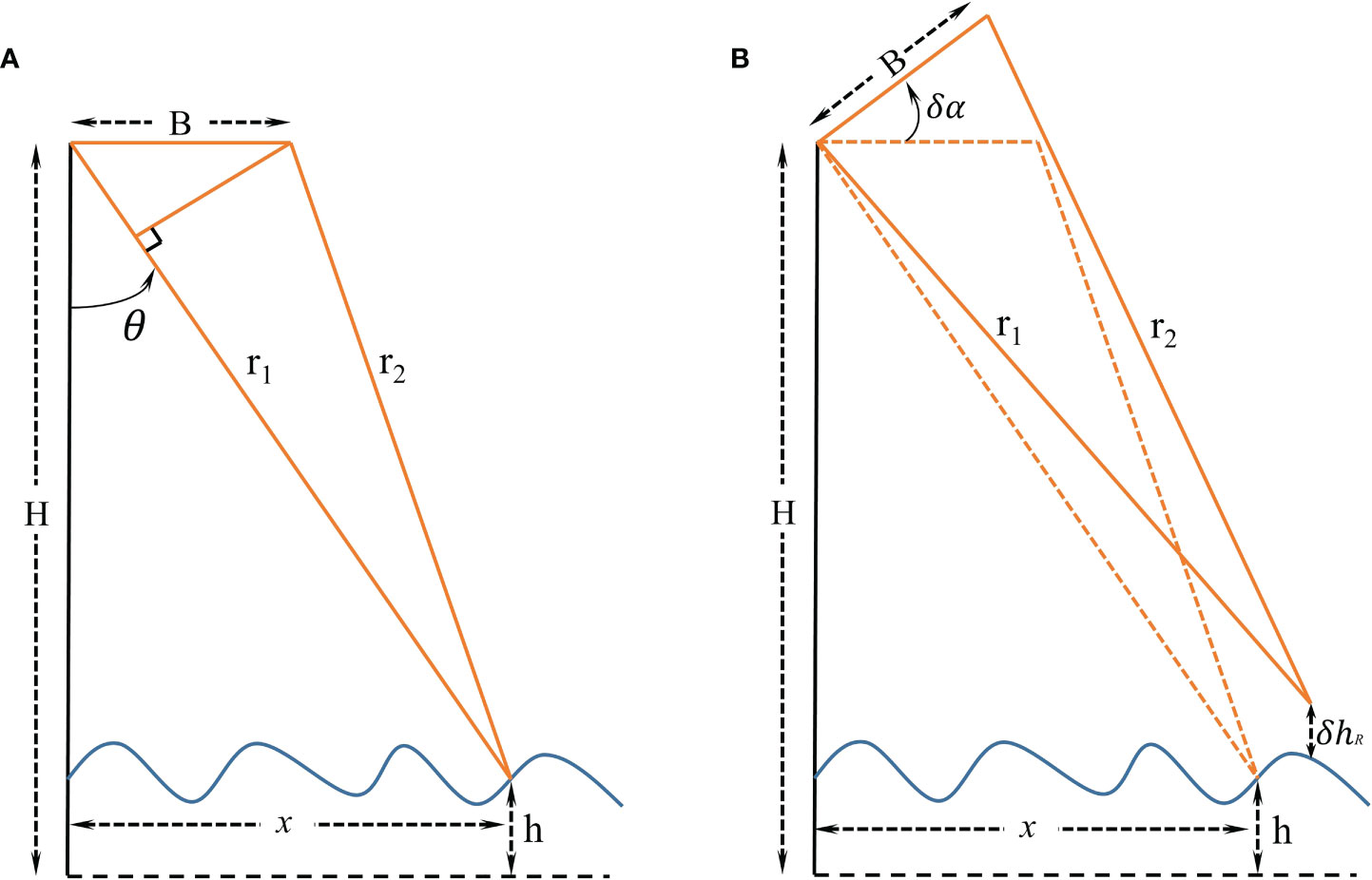
Figure 3 Interferometric measurement concept (A) and the illustration of the impact of baseline roll error on height measurement (B).

where x represents the observation position in the cross-track direction, and δB refers to the baseline length measurement error. When the roll error is δα, as shown in Figure 3B, the HEBR (δh_R) can be obtained by following equation (Dibarboure et al., 2012).

$\begin{array}{ll}\delta h_R=x*\delta \alpha & (6)\end{array}$

The errors are related to the position along the track and across the track. In our method, functions of time t (corresponding to the position in the along-track direction) and x (position of the measurement in the cross-track direction) are applied. For a given point on the swath, the observation H_obs(x, t) of “Guanlan” is the sum of the “true SSH” H_real(x, t) and errors. The H_real(x, t) comes from the HYCOM model and errors include HEBL (δh_B), HEBR (δh_R) and other uncorrected errors ϵ(x, t). H_obs(x, t) corresponding to Guanlan_1 (H_obs1(x₁, t₁)) and Guanlan_2 (H_obs2(x₂, t₂)) are calculated as follows:

$\begin{array}{ll}{H}_{obs1}\left(x_1,t_1\right)=H_{real1}\left(x_1 ,t_1\right)+x_1*\delta \alpha \left(t_1\right)+x_1^2*\frac{\delta B\left(t_1\right)}{H*B}+{ϵ}_1(x_1,t_1)& (7)\end{array}$

$\begin{array}{ll}{H}_{obs2}\left(x_2,t_2\right)=H_{real2}\left(x_2 ,t_2\right)+x_2*\delta \alpha \left(t_2\right)+x_2^2*\frac{\delta B\left(t_2\right)}{H*B}+{ϵ}_2(x_2,t_2)& (8)\end{array}$

In overlapping-calibration method, a given point (lon, lat) located in the overlapping swath can be observed twice in a short time (240s), and the differences between H_real1 and H_real2 in two satellites can be ignored. Therefore, the different (Y(lon, lat)) between the two observations at this point (lon, lat) can be calculated with the equation below.

$\begin{array}{ll}\begin{array}{l}Y\left(lon,lat\right)=H_{obs1}\left(lon,lat\right)-H_{obs2}\left(lon,lat\right)\hfill \\ =H_{obs1}\left(x_1,t_1\right)-H_{obs2}\left(x_2,t_2\right)\hfill \\ =x_1*\delta \alpha \left(t_1\right)-x_2*\delta \alpha \left(t_2\right)+x_1{}^2*\frac{\delta B\left(t_1\right)}{H*B}-x_2{}^2*\frac{\delta B\left(t_2\right)}{H*B}+ {ϵ}_1(x_1,t_1)- {ϵ}_2(x_2 ,t_2)\hfill \\ =x_1*\delta \alpha \left(t_1\right)-x_2*\delta \alpha \left(t_2\right)+x_1{}^2*\frac{\delta B\left(t_1\right)}{H*B}-x_2{}^2*\frac{\delta B\left(t_2\right)}{H*B}+ \delta ϵ\hfill \end{array}& (9)\end{array}$

where H_obs1(x₁, t₁) and H_obs2(x₂, t₂) represent the observation of Guanlan_1 and Guanlan_2 respectively. The equation (9) converted into the matrix form is equation (10):

$\begin{array}{ll}Y=\left[\left(x_1\right) \left(\frac{x_1{}^2}{H*B}\right) \left(-x_2\right) \left(-\frac{x_1{}^2}{H*B}\right)\right] \left[\begin{array}{c}\delta \alpha \left(t_1\right)\\ \delta B\left(t_1\right)\\ \begin{array}{c}\delta \alpha \left(t_2\right)\\ \delta B\left(t_2\right)\end{array}\end{array}\right]+\delta ϵ& (10)\end{array}$

Here, M is introduced as the observation model mapping the state space to the observed space (linear or quadratic signature models), as shown in equation (11).

$\begin{array}{ll}M = \left[\left(x_1\right) \left(\frac{x_1{}^2}{H*B}\right) \left(-x_2\right) \left(-\frac{x_1{}^2}{H*B}\right)\right]& (11)\end{array}$

An optimal inverse method is introduced by equation (12), where R_est is the estimated vector of δα(t) and δB(t):

$\begin{array}{ll}{R}_{est}= {\left(M^T· M\right)}^{-1}· M^T·Y& (12)\end{array}$

Formula 12 gives the general form of the least-squares method of error estimation for 4 parameters (i.e., δα(t₁), δα(t₂), δB(t₁) and δB(t₂)). This method for estimating δB and δα was first proposed by (Dibarboure et al., 2012) and is planned to be employed in SWOT mission. Furthermore, we propose an improved overlapping-calibration method based on a short time interval two-satellite flying design, the detailed orbits, error terms and OSSEs design are described in section 3. In practical applications, these 4 parameters are expected to be as small as possible. Particularly, both length errors are likely to be able to satisfy the requirements of “Guanlan” mission through high-precision measurement methods. Therefore, if it is found that some of the 4 parameters are small enough, then the corresponding parameters of the error in the M matrix can be set to 0 without estimation. For example, when the inputting baseline roll errors (δα(t₁), δα(t₂)) of Guanlan_1 and Guanlan_2 are ~1 arcsec, and the precision of baseline length can reach ~12μm, the HEBL will be maintained very small. In this case, it is unnecessary to estimate δB(t₁) and δB(t₂), and thus M will be set as [(x₁)(0)(-x₂)(0)]. As a result, R_est will only include the estimation results of δα(t₁) and δα(t₂).

3 Observing system simulation experiments

3.1 Orbit design

As shown in Figure 1, the satellite in the front is named “Guanlan_1”, and the other is “Guanlan_2”. As presented in Table 1, the parameters of their orbits are listed.

TABLE 1

Table 1 Parameters of orbits.

The orbit design of “Guanlan_1” references to the orbit parameters of “Guanlan” mission (Chen et al., 2019), and the parameters of “Guanlan_2” are the same as those of “Guanlan_1” except for the “Epoch”. The epoch of a spacecraft is the time corresponding to the orbital initial conditions. The difference of “Epoch”, which keeps the two satellites flying at a certain time interval, can be adjusted so that their swaths on the ground can be partially overlapped. The average overlapping swath width in the experimental region (80°W- 180°W, 0°S- 20°S) is 85 km. Figure 4 shows the ground track of these two satellites with the interval of 240 seconds in a cycle.

FIGURE 4

Figure 4 The ground track of “Guanlan_1” and “Guanlan_2” with 240s interval.

3.2 “Guanlan” observation simulation

As described in the document of SWOT error budget (Peral and Esteban-Fernandez, 2018), there are various error sources, including systematic error, random noise, and media error. The details can be found at “https://swot.jpl.nasa.gov/resources/documents/”. “Guanlan” satellite has similar error sources. In this study, the purpose of this study is to demonstrate the feasibility of the overlapping-calibration technique on topography products, assuming that all scientific requirements are met on Guanlan’s error budget except SSH_Error_Baseline. As a result, three types of inputting errors, including HEBR, HEBL and RN, are simulated.

The spatial distribution of inputting errors and the “true SSH” have been shown in Figure 5. As shown in Figures 5A-C, three inputting (HEBR, HEBL and RN) errors are simulated, and they are mainly kept below 1 cm respectively. The variation of the HEBR and HEBL in the along-track direction are synthesized through the SSH_Error_Baseline spectrum, which can be obtained using the software of the SWOT simulator (Gaultier et al., 2016; Chaudhary et al., 2021). The inputting errors of Guanlan_1 and Guanlan_2 are similar. When both the wide-swath altimeter payload noise and SSH_Error_Baseline can satisfy the design requirement as presented in Figures 5A–C, the corresponding SSH observation is displayed in Figure 5E. The observation looks like the sampled SSH model data (Figure 5D), since the ocean SSH signal is much larger than the total errors. If the noise and errors are so small, the “Guanlan” mission will be successful and the mesoscale ocean eddy in the blue box will be easily detected (Durand et al., 2010; Ma et al., 2020).

FIGURE 5

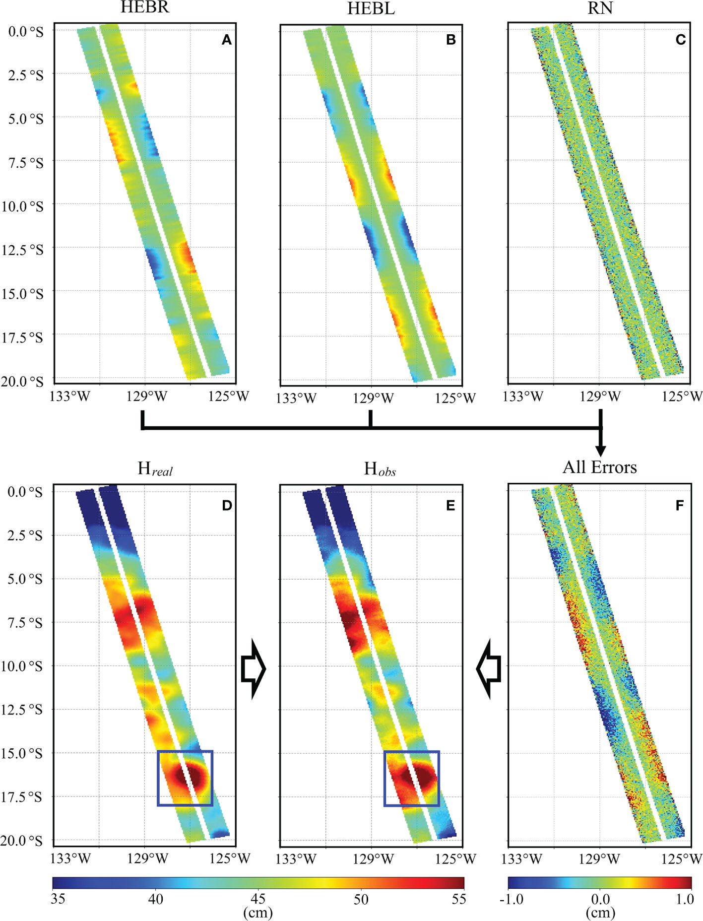
Figure 5 Error sources and observation simulation of “Guanlan” mission: (A-C) are SSH error due to baseline roll error (HEBR), baseline length error (HEBL), and random noise (RN) respectively; (F) is the total error contained in satellite observation; (D, E) is the true SSH/SSH observed by “Guanlan”.

3.3 Experimental setup

The width of overlapping swath varies with the time interval between two satellites. When the time interval is set to 240 s, the average width of overlapping swaths in the experimental region is 85 km that is half of the effective swath (170 km) of “Guanlan” mission. In such case, the average united swath width about 255 km, and thus the loss of ocean sampling capabilities is 25% (1- 255/340).

Based on equation (5) and equation (6), we consider the HEBR and HEBL at the 100 km outer edge position to be less than 1 cm in order to satisfy the requirement. Therefore, the precision of the baseline roll error should be less than 0.02 arcsec, while that of the length error should be less than 12 μm. Moreover, this study aims to reveal the error reduction capability of two-satellite formation flight design under the pessimistic theoretical scenario of baseline roll and length errors. Therefore, the measurement accuracy of baseline rolling is set to 1 arcsec by default, and that of baseline length is assumed to be 0.6 mm, which are almost 50 times worse than the values mentioned in section 3.2. In this study, a total of 9 different pessimistic theoretical scenarios, namely OSSEs_1 to OSSEs_9, are sorted out. Corresponding setups are listed in Table 2. Furthermore, the P= (%) is calculated based on the equation (13), error∈(HEBR₁,HEBL₁, HEBR₂, HEBL₂) , where HEBR/HEBL represents the baseline roll/length error and RN represents the random noise.

TABLE 2

Table 2 The settings of all OSSEs.

$\begin{array}{ll}{\text{ P}}_{\text{error}}=\frac{100*\text{error}}{\left({\text{HEBR}}_1+{\text{HEBL}}_1+{\text{RN}}_1+{\text{HEBR}}_2+{\text{HEBL}}_2+{\text{RN}}_2\right)}& (13)\end{array}$

In this study, 9 types of pessimistic theoretical scenarios are listed by setting whether the baseline parameters can satisfy the expected requirements, when all the anomalies that may occur on the baselines of the two satellites are covered. OSSEs_1 to OSSEs_2 correspondingly simulated the scenarios that a satellite with insufficient baseline length or roll measurement precision of Guanlan_2, whereas OSSEs_3 to OSSEs_6 refer to 4 types of combinations of two baseline parameters with low accuracy. In the experiments of OSSEs_7 and OSSEs_8, only one parameter that is the baseline length and roll of Guanlan_1, can still achieve the expected accuracy. Beyond that, OSSEs_ 9 describes the most pessimistic scenario, while the precision of 4 baseline parameters belonging to the two satellites cannot simultaneously reach the expected goal. Moreover, in order to facilitate the experiments, default accuracies are given respectively in Table 2, and the actual parameters in the future are currently uncertain. In addition, M parameters corresponding to OSSEs_1 to OSSEs_9 are different and listed in Table 2. For example, as only two HEBRs are required to be estimated in the OSSEs_4, M is set to [(x₁) 0 (−x₂)  0] . However, OSSEs_9 simulates the worst situation that all the baseline parameters of Guanlan_1 and Guanlan_2 failed to satisfy the requirements. The OSSEs_9 should estimate 4 error parameters, and thus M is set to $\left[\left(x_1\right)\left(\frac{x_1^2}{\text{H}*\text{B}}\right)\left(-x_2\right)\left(-\frac{x_2^2}{\text{H}*\text{B}}\right)\right]$. In the Guanlan mission, the baseline length measurement accuracy can reach 12 μm, while it is really too difficult to achieve the baseline rolling measurement accuracy of 0.02 arcsec. Therefore, the current baseline accuracies of the Guanlan are designed close to the scenarios shown in OSSEs_4 rather than OSSEs_9.

4 Results

4.1 SSH_Error_Baseline reduction results of OSSEs_1 and OSSEs_2

Figure 6 shows the SSH_Error_Baseline reduction results when the baseline length/roll accuracy of Guanlan_2 is set to 0.6 mm/1 arcsec in OSSEs_1/OSSEs_2 respectively. The true SSH (H_real), observed SSH (H_obs), and calibrated results (H_cal) are plotted from left column to right column. And the overlapping swath is labeled with black dotted lines, which is 85km corresponding to the 240s time interval between the two satellites. The pattern of observed SSH follows the quadratic (Figure 6B) and linear (Figure 6E) relationship in the cross-track direction, which is consistent with the function of error model in equation (5) and (6). And the calibrated results are similar to the true SSH, which means that most of ocean signals have been recovered.

FIGURE 6

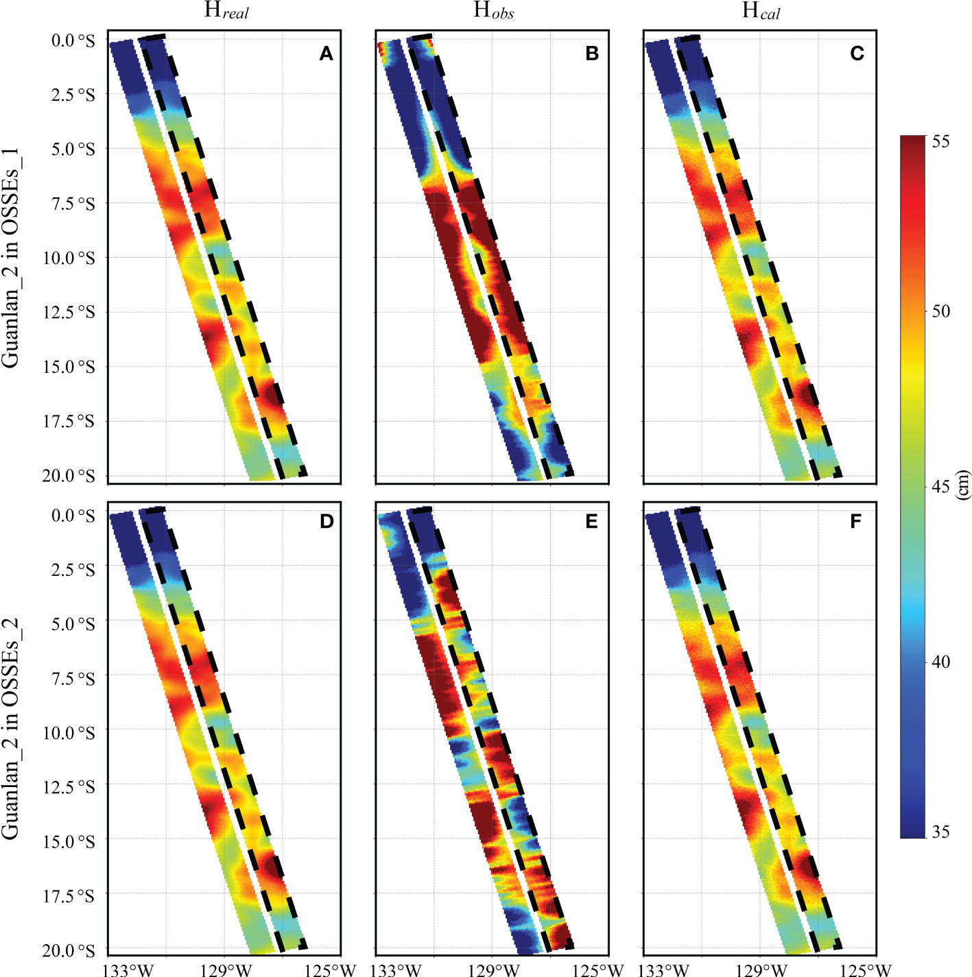
Figure 6 SSH_Error_Baseline reduction results in OSSEs_1 (A-C) and OSSEs_2 (D-F). Each column shows the true SSH, observed SSH and the calibrated results from left to right.

The details of the residual errors of OSSE_1 and OSSE_2 are shown in Figure 7. The average RMS of residual errors in the cross-track direction are almost less than 1cm both in OSSE_1 (Figure 7A) and OSSE_2 (Figure 7D). Meanwhile, the average RMS of residual errors in the no overlapping regions (by red lines) are larger than that of residual errors located in the overlapping regions (by purple lines). The distribution of the residual errors is plotted by calculating the difference between the true SSH (H_real) and calibrated results (H_cal) shown in Figure 6. And the maximum residual errors vary between 0.8cm to 1cm along the bold red lines in Figures 7B, D. Then, the variation of residual errors along the bold red lines are plotted in Figures 7C, F. In these two sub-figures, the black lines present the inputting HEBR/HEBL, the blue lines present the residual HEBL/HEBR after calibration, and the red lines present the total residual errors. Taking OSSEs_1 as an example, the residual error at the far end of the swath is only about 0.5cm when the HEBR is approximately 0.1cm (by dotted orange line in Figure 7C). By contrast, the residual error can reach 1.7cm when the HEBR is 0.5cm (by dotted green line in Figure 7C). Therefore, it can be found that the total residual errors are positively associated with the inputting HEBR/HEBL.

FIGURE 7

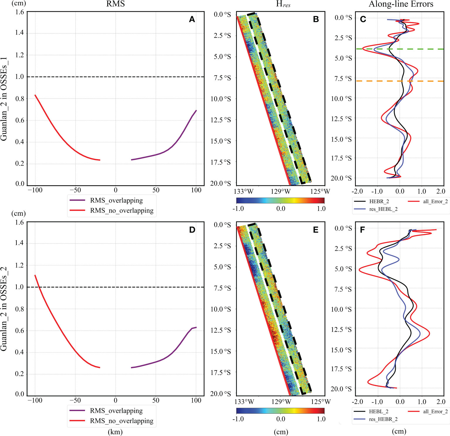
Figure 7 Residual errors of Guanlan_2 in OSSE_1 (A–C) and OSSE_2 (D–F). (A, D) is the average RMS of residual errors in the cross-track direction, (B, E) is the distribution of the residual errors, and (C, F) displays various errors along the bold red lines in (B, E).

4.2 SSH_Error_Baseline reduction results from OSSEs_3 to OSSEs_6

The OSSEs_3 to OSSEs_5 simulate the pessimistic theoretical scenarios that the accuracy of one of the baseline parameters on each satellite is low. By applying the process of overlapping-calibration, the residual errors can almost be reduced to less than 1 cm.

The Figure 8 shows the reduction errors of OSSEs_3. In the OSSEs_3, the baseline roll accuracies of both satellites are very high, while the length accuracies are down to 0.6 mm, and thus the HEBL of both satellites should be calibrated. As shown in Figures 8A, D, the mean RMS of the residual of Guanlan_1 and Guanlan_2 increases with the distance from nadir in the cross-track direction. Moreover, the largest RMS of the residual is also less than 1 cm and located in the non-overlapping swath, as marked with a bold red line in Figures 8B, E. Furthermore, the components of residual errors along these red lines are plotted in Figures 8C, F. Similar to the above-mentioned results in OSSEs_1 and OSSEs_2, the residual errors are positively related to the inputting errors (black lines in Figures 8C, F), which are HEBRs in the current experiment.

FIGURE 8

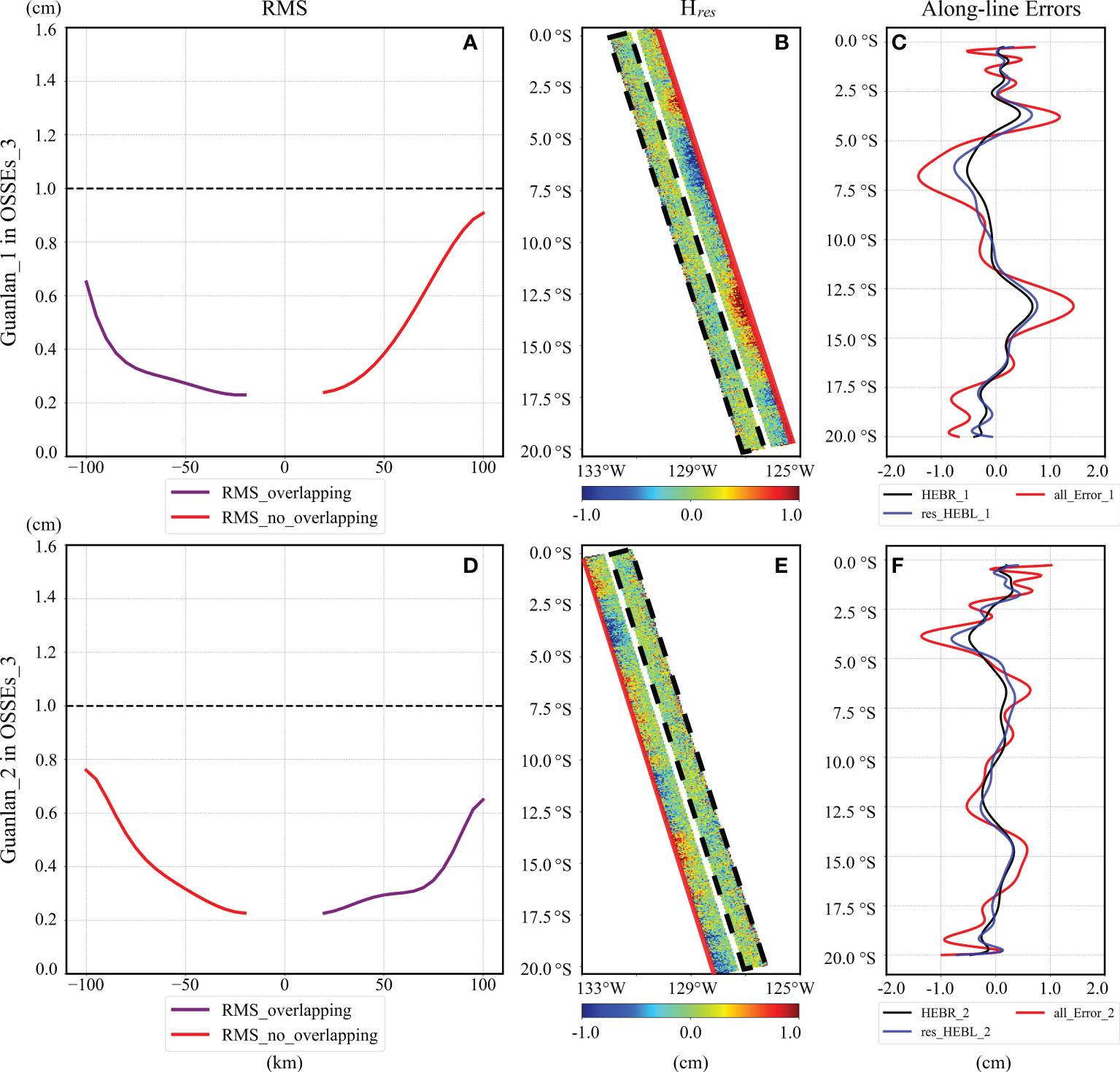
Figure 8 Reduction errors of OSSEs_3: (A, D) plots the average RMS of residual errors of Guanlan_1 and Guanlan_2 in OSSEs_3; (B, E) shows the residual errors on the swath of Guanlan_1 and Guanlan_2 in OSSEs_3; (C, F) displays various errors along the bold red lines in (B, E).

The reduction errors of OSSEs_4 and OSSEs_5 are shown in Figures 9. The simulation scenarios in OSSEs_4 are probably to appear, because it is really a huge challenge for the engineer to maintain the accuracy of baseline rolls at the level of 0.02 arcsec. In the OSSEs_4, the baseline roll accuracies of Guanlan_1 and Guanlan_2 are set as 1 arcsec, which can be achievable. Furthermore, the observation results are similar to that illustrated in Figure 6E. Based on the overlapping-calibration method proposed in this study, the residual errors are shown in Figures 9A, B. In addition, the patterns of residual errors are similar to OSSEs_3, and the RMS of the residual of Guanlan_1 and Guanlan_2 can almost be controlled within 1 cm. Apart from that, the Guanlan_1 calibration results (Figure 9D) of OSSEs_5 seem like the results of the Guanlan_1 of OSSEs_4 (Figure 9B). Meanwhile, the Guanlan_2 calibration results (Figure 9C) of OSSEs_5 are similar to those of Guanlan_2 of OSSEs_3 (Figure 8D). As expected, the residuals can still be controlled within 1 cm on the united swath.

FIGURE 9

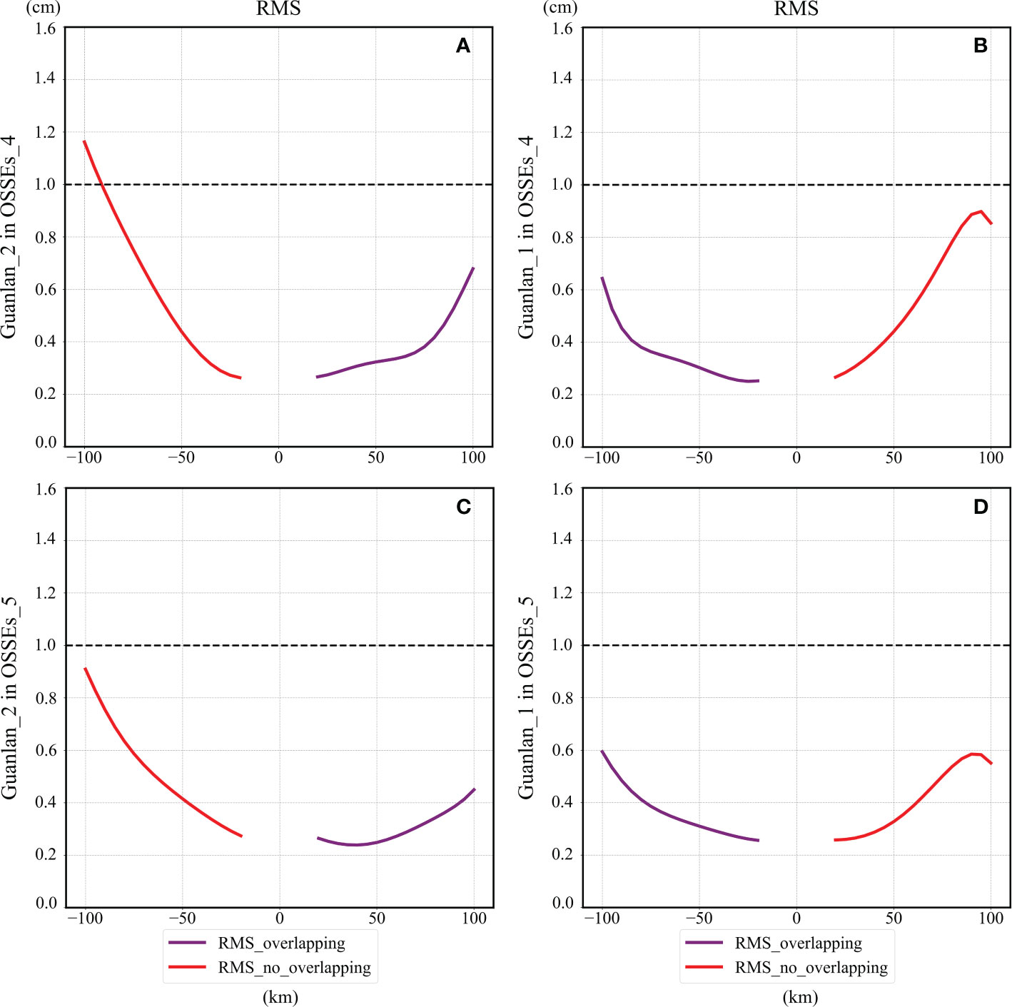
Figure 9 Reduction errors of OSSEs_4 and OSSEs_5: (A, B) plots the average RMS of residual errors of Guanlan_2 and Guanlan_1 in OSSEs_4, while (C, D) shows that in OSSEs_5.

The Figure 10 shows the calibration results of OSSEs_6, which simulates a scenario, that is, baseline roll and length anomalies occur simultaneously on one satellite. In this experiment, the baseline roll (length) error accuracy of Guanlan_2 is set as 1 arcsec (0.6 mm). As a result, the maximum error may be more than 50 cm based on formulas 1 and 2. In addition, there are two parameters of Guanlan_2 that need to be estimated, and M is set to $\left[00\left(-x_2\right)\left(-\frac{x_2^2}{\text{H}*\text{B}}\right)\right]$. In such case, the calibration results are shown in Figure 10. In such case, the residual errors in the overlapping and the non-overlapping areas are significantly different, as displayed in Figures 10A, B. In the overlapping region, the mean RMS of the residual is less than 0.8 cm, but in non-overlapping areas, it has reached 4.2 cm, approximately 5 times that of overlapping areas (Figure 10A). The difference can be explained from Figures 10C, D. In the overlapping (non-overlapping) area, the calibrated roll and length errors show a significantly negative (positive) correlation, generating a decrease (an increase) in the total error.

FIGURE 10

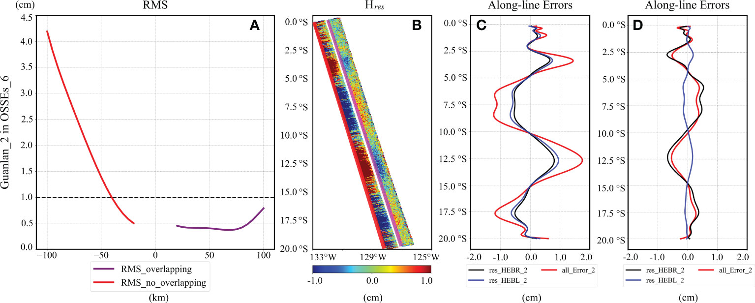
Figure 10 Reduction errors of OSSEs_6: (A) plots the average RMS of residual errors of Guanlan_2 in OSSEs_6; (B) shows the residual errors on the swath of Guanlan_2 in OSSEs_6; (C, D) indicates various errors along the bold red (purple) lines in (B).

In addition, we plot the distribution of the residual errors along the cross-track direction for OSSEs_6, as shown in the Figure 11. The right shadow represents the overlapping area, where the signs of the residual baseline length error (res_HEBL_2, blue line) and the residual baseline roll error (res_HEBR_2, black line) are almost opposite. The total error decreases after the addition of positive and negative values. However, the errors in non-overlapping areas (unshaded parts of Figure 11) are all positive, and the total error increases after addition. Therefore, in the overlapping (non-overlapping) area, the residual roll and length errors show a significantly negative (positive) correlation, which leads to a decrease (an increase) in the total error. Both baseline errors (HEBR, HEBL) are summed in the non-overlapping region when they are in the pessimistic scenario simultaneously, which leads to larger residual errors in OSSEs_6 than that of OSSEs_1 to OSSEs_5.

FIGURE 11

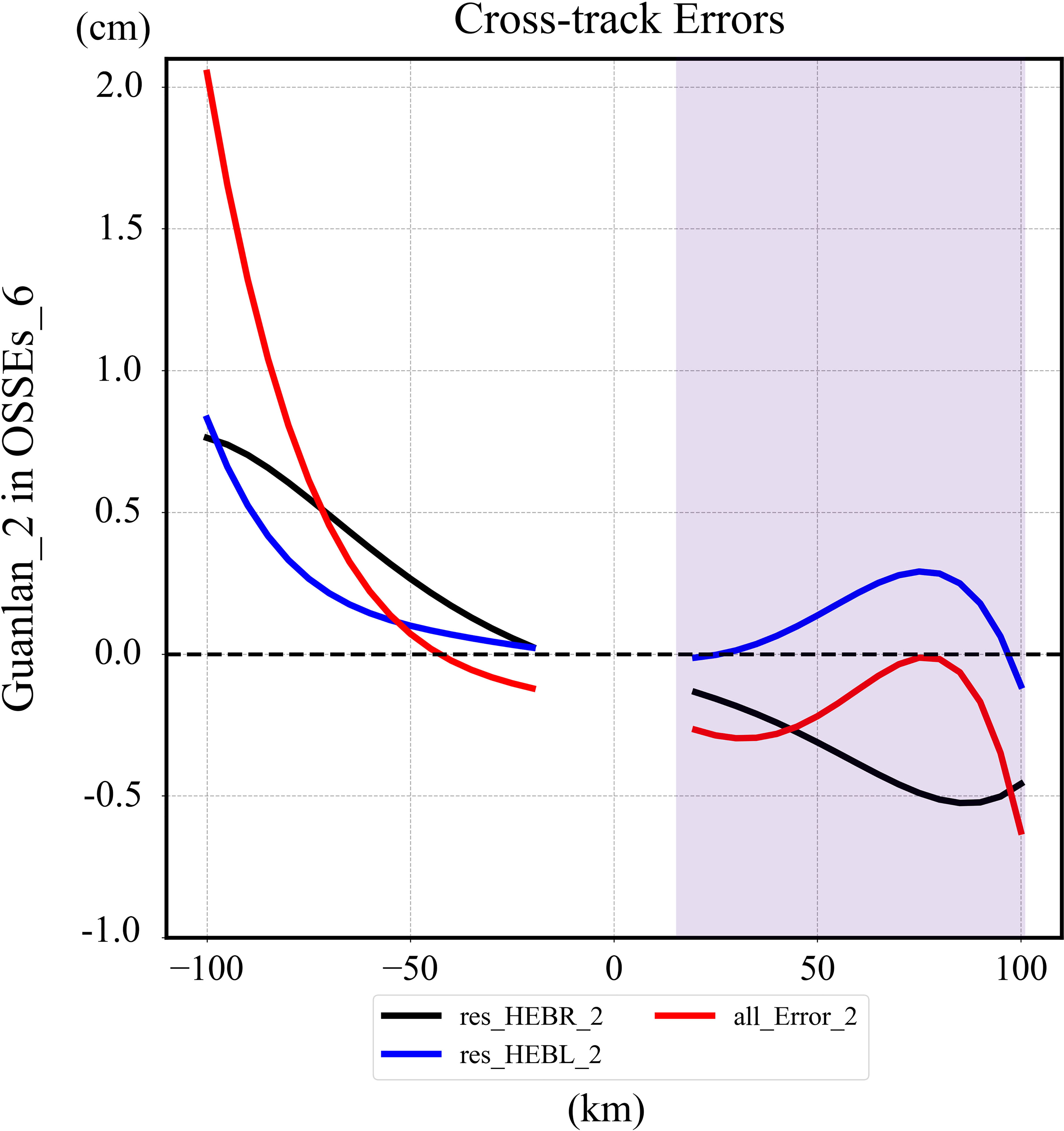
Figure 11 The reduction errors of OSSE6 overlapping area (right shadow) and non-overlapping area (left) in the direction of cross-track. It shows the variation of residual baseline length error (res_HEBL_2, blue line), the residual baseline roll error (res_HEBR_2, black line) and total error (all_Error_2, red line) in cross-track direction.

In this study, the residual SSH_Error_Baseline is required to be less than 1 cm, and the corresponding swath excluding the intermediate gap is called the “effective swath”. Therefore, only the data at the location with a distance of less than 40 km from the nadir point can satisfy the accuracy requirements in the non-overlapping area. Here, the expression of [a, b] is employed to indicate the range of the effective swath, while the variable a (b) indicates the position of the left (right) boundary of the effective swath, and is represented by a negative (positive) number. Under the pessimistic scenario of OSSEs_6, the SSH_Error_Baseline of the data in the area [-40km, 100km] of the Guanlan_2 swath can be reduced to less than 1 cm. Hence, it can be guaranteed that approximately 65% observation of Guanlan_2 is valuable based on the two-satellite formation flying design.

4.3 SSH_Error_Baseline reduction results from OSSEs_7 to OSSEs_9

OSSEs_7 (OSSEs_8) simulates the situation that the accuracy of the three parameters, namely the baseline roll and length of Guanlan_2 and the baseline roll (length) of Guanlan_1 cannot satisfy the high accuracy requirements.

The initial values of each parameter are listed in Table 2, and the calibration results of OSSEs_7 are shown in Figure 12. The mean RMS of most residual errors, shown in Figure 12A, is less than 1 cm, and the effective swath range of Guanlan_1 in the cross-track direction is [-100km, 90km], while the residual error of Guanlan_2 is larger than that of Guanlan_1, and the effective swath of Guanlan_2 is [-40km, 100km]. Since these two satellites have an overlapping area of 85 km, the combined observation swath of them is 185 km.

FIGURE 12

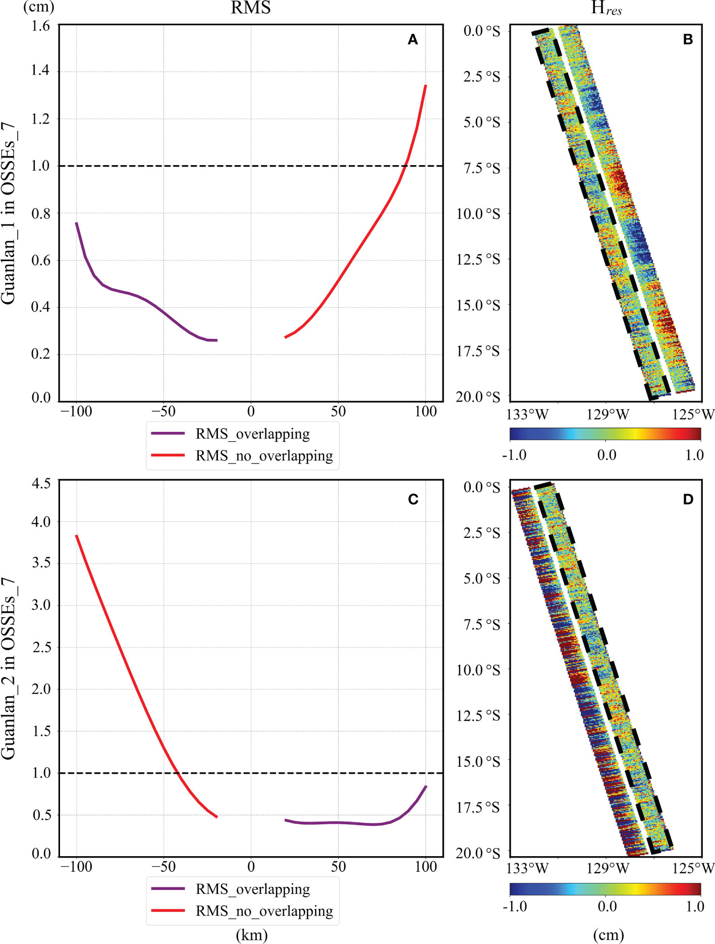
Figure 12 Reduction errors of OSSEs_7: (A, C) plots the average RMS of residual errors of Guanlan_1 and Guanlan_2 in OSSEs_7; (B, D) shows the residual errors on the swath of Guanlan_1 and Guanlan_2 in OSSEs_7.

The calibration results of OSSEs_8 are similar to those of OSSEs_7, as shown in Figure 13A, B. It can be found that the residual error of Guanlan_2 in OSSEs_8 is also larger than that of Guanlan_1. Apart from that, the effective swath range of Guanlan_1 in the cross-track direction is [-100km, 90km], and that of Guanlan_2 is [-45km, 100km]. As a result, the combined observation swath of the two satellites is slightly larger and is approximately 190 km. Furthermore, OSSEs_9 simulates the worst situation that all the baseline parameters of Guanlan_2 and Guanlan_1 failed to satisfy the requirements settings described in section 3.3. The RMS of residual errors in the overlapping area of OSSEs_9 are plotted by the purple lines for Guanlan_1 (Figure 13C) and Guanlan_2 (Figure 13D), which ranges from 1 cm to 4 cm. Therefore, if the error budget of SSH_Error_Baseline cannot exceed 1 cm, the data in the case of OSSEs_9 will all be invalid.

FIGURE 13

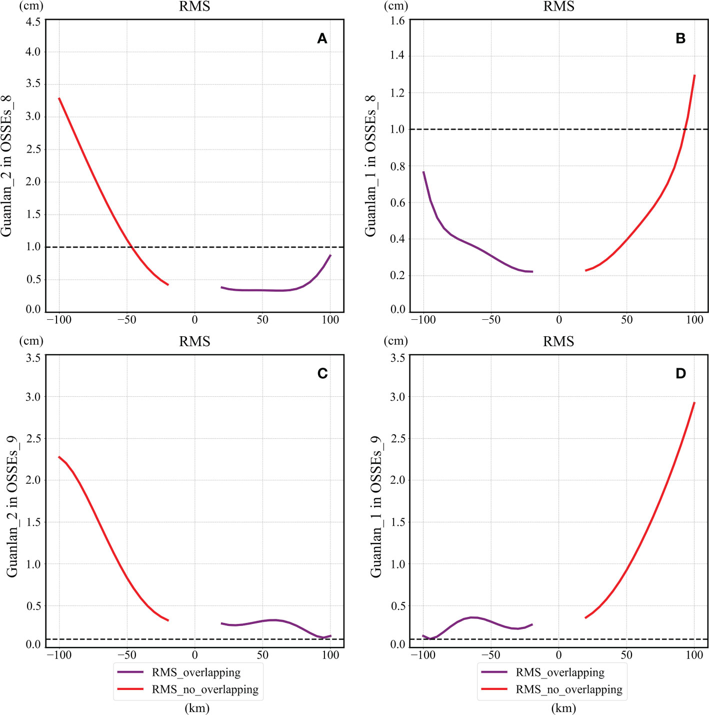
Figure 13 Reduction errors of OSSEs_8 and OSSEs_9: (A, B) plots the average RMS of residual errors of Guanlan_2 and Guanlan_1 in OSSEs_8; (C, D) shows that in OSSEs_9.

4.4 Wavenumber spectrum and the effective width of the united swath

In the above OSSEs, the swath where the average RMS of the residual is less than 1 cm is regarded as the “effective swath”. We have validated such evaluation criterion in the spectral domain by making wavenumber spectrum analysis. The wavenumber spectrum of the “true SSH” from the model data (H_real, with red line) and the calibrated SSH (H_cal, with black line) with RMS less than 1 cm are plotted in Figure 14. As a result, the black line follows the red line until ~17 km, indicating that the threshold of 1 cm corresponds to the resolvable scale of ~17 km after calibration.

FIGURE 14

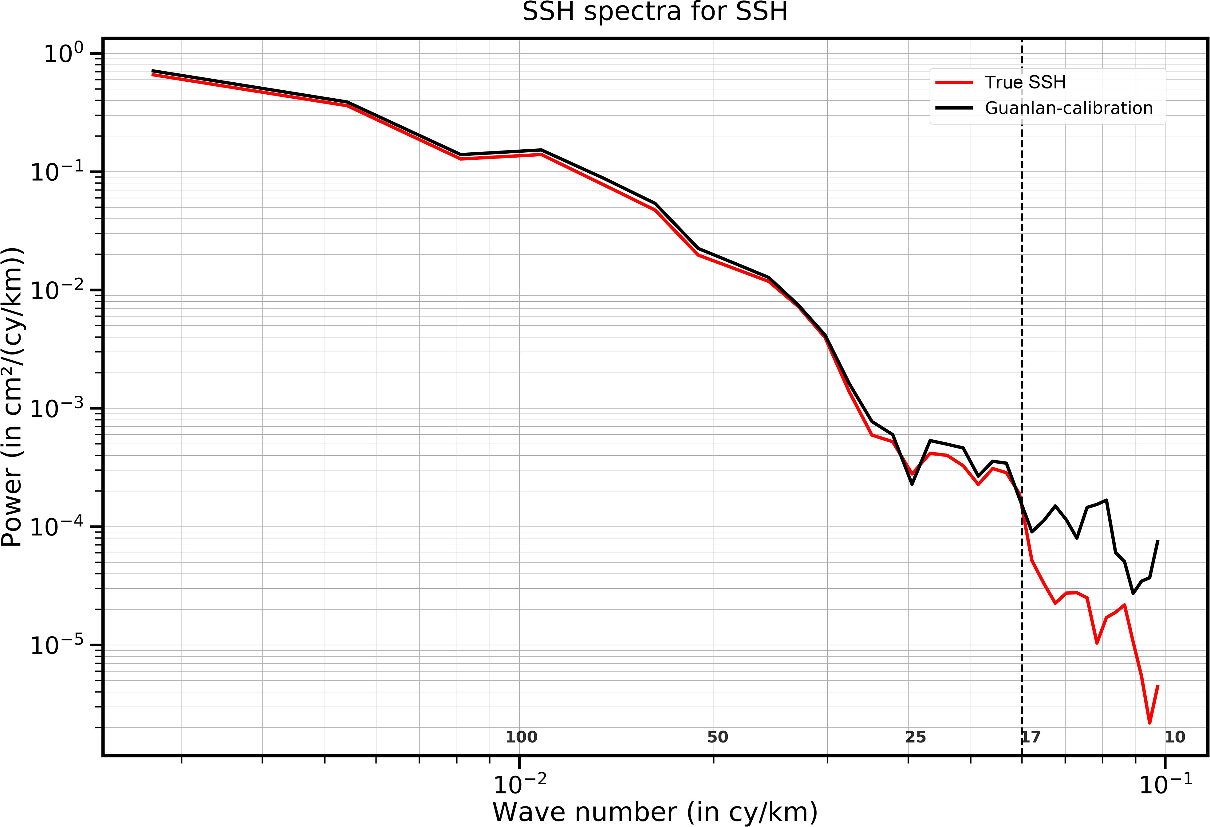
Figure 14 Wavenumber spectrum of the true SSH data (red), and the calibration SSH in the effective swath with 1 cm threshold (black).

Table 3 lists the effective width of swath for Guanlan_1, Guanlan_2, and the united swath after overlapping in the 9 experiments. The effective width of swath after overlapping has been excluded the width of middle gap (30 km). Specifically, the effective swath width of OSSEs_1 to OSSEs_5 can basically cover the whole observation area, and it is nearly 250 km. Since there are three baseline parameters in OSSEs_6 to OSSEs_8 that do not satisfy the requirements, the effective swath width will be reduced to 185~195 km. When the four parameters fail to satisfy the requirements, just like the setting of OSSEs_9, the effective swath width will suddenly drop to 0 km.

TABLE 3

Table 3 The effective swath width of two satellites after overlapping-calibration.

5 Discussions

5.1 Sensitivity of baseline accuracy

In order to analyze the sensitivity of the baseline accuracy to the experimental results, additional seventeen sets of experiments have been designed and conducted. In the Table 4, there are four inputting paramaters (N_{roll_Guanlan_1}, N_{length_Guanlan_1}, N_{roll_Guanlan_2}, N_{length_Guanlan_2}), and each parameter represents the corresponding multiple of the current accuracy relative to the required accuary. Based on the known required baseline roll/length accuracy(0.02 arcsec/12 μm, from in section 3.3), we can easily calculate the inputting baseline accuarcies. Take OSSEse N_{roll_Guanlan_1}, N_{length_Guanlan_1}, N_{roll_Guanlan_2}, N_{length_Guanlan_2}) is set as (1,1,1,100), the vector of (Accuracy_{roll_Guanlan_1}, Accuracy_{length_Guanlan_1}, Accuracy_{roll_Guanlan_2}, Accuracy_{length_Guanlan_2}) is equal to (1*0.02 arcsec, 1*12 μm, 1*0.02 arcsec, 100*12 μm). The value of N in Table 4 can be interpreted as follows:

● N=1: the baseline roll/length accuracy meets the requirements (baseline roll/length accuracy is equal to 0.02 arcsec/12 μm),

● N=2: the baseline roll/length accuracy is twice lower than the corresponding requirement (baseline roll/length accuracy is equal to 0.04 arcsec/24 μm),

● N=50: the anomaly of baseline roll/length accuracy is same as that of the OSSEs in section 3.3 (baseline roll/length accuracy is equal to 1 arcsec/600 μm),

● N=100: the anomaly of baseline roll/length accuracy is twice larger than that of the OSSEs in section 3.3 (baseline roll/length accuracy is equal to 2 arcsec/1200 μm).

TABLE 4

Table 4 Baseline residual errors with different magnification.

These additional experiments have employed the same inputting model data and overlapping-calibration method as the OSSEs in section 2 and 3. The value of “effective width of united swath (EWUS)” of every experiment has been calculated.

In the Table 4, the experiment represented by the OSSEs_i_j is derived from the setting in OSSE_i, which is regarded as the “reference experiment”. The EWUS in OSSEs_i_j must be smaller than that in OSSEs_i because the inputting errors of OSSEs_i_j are larger. As a result, the reduced EWUS of every experiment has been listed in the last column of Table 4. Compared with the “reference experiment”, EWUS of the OSSEs_i_1 does not decrease, while the results of the OSSEs_i_2 show that the EWUS is reduced. Therefore, it can be concluded that when the baseline roll/length accuracy is twice lower than the corresponding requirement, the effective width of the united swath will be reduced with the overlapping-calibration method. Among them, the EWUS of OSSEs_3_2, OSSEs_4_2 and OSSEs_5_2 are reduced by 45km, 55km and 50km respectively. In other words, when the accuracy of one of the baseline parameters on each satellite is low, the correction results will be very sensitive to the change of baseline accuracy.

5.2 Correlation between residuals and latitude

The width of the overlapping area is associated with the latitude. Here, we add experiments to explore the influence of latitude on the residuals. This supplemental experiment has two limitations. One is that only OSSEs_1- OSSEs_8 are analyzed, because our method is invalid in OSSEs_9 (all the SSH_Error_Baseline did not satisfy the requirements). Another is that the latitude range is only extended to 66°S (latitude of the Antarctic circle) instead of 90°S. The polar regions are not discussed in this study. In addition, the calibration results of OSSEs conducted in this study are not related to longitude and sea state. At first, the calibration results of “two-satellite formation flying design” are related to the width of overlapping swath, which only varies with latitude. Considering the symmetry of the overlapping swath in the northern and southern hemispheres as well as the uncorrelation with longitude, the Pacific experiments (0°S-66°S) can replace global experiments concerning latitude and longitude range. Second, SSH variation and sea states in different regions appear to propagate in the estimated solutions of δB and δα through δϵ in equation (10). Based on the proposed overlapping-calibration method, the SSH time variation can be neglected. In addition, the impact of the sea states on the random noise is not discussed in this study. Therefore, the results in the South Pacific can well illustrate the calibration ability of the proposed algorithm, and it is not essential to carry out the global coverage experiments.

Therefore, we have plotted the width of overlapping swath varying with latitude and the residual errors varying with latitude for OSSEs_1 to OSSEs_8 in Figure 15. As shown in the Figure 15A, the width of the overlapping area decreases slightly and subsequently increases rapidly with increasing latitude. In the range of 0°S -52°S, the average width of the overlapping area is about 85 km, with a variation of less than 10 km. The width increases rapidly when it is higher than 52°S, reaching the maximum of 175 km at 66°S.

FIGURE 15

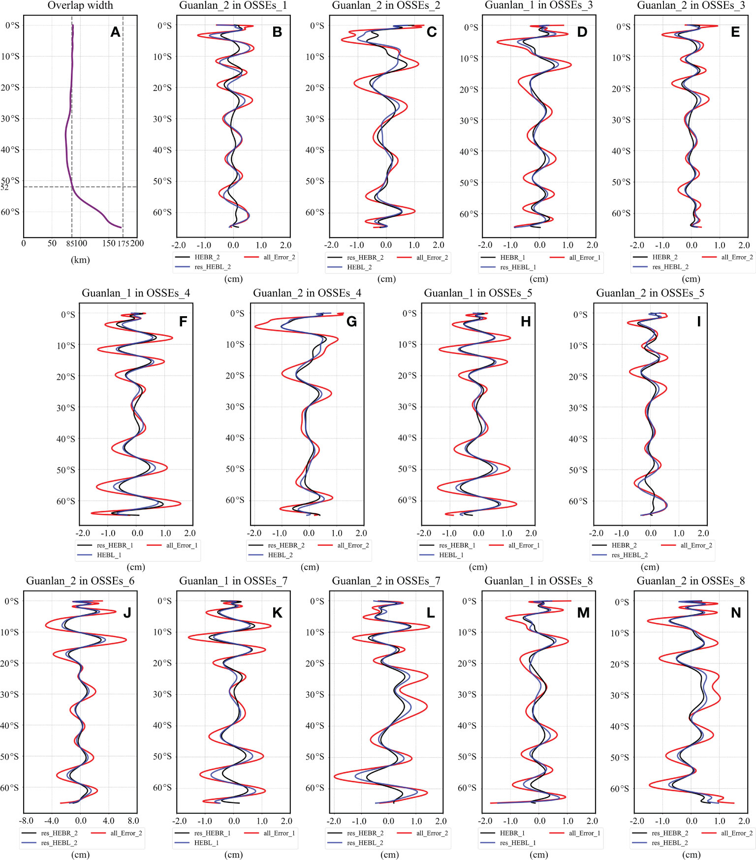
Figure 15 (A) shows the variation of the width of overlapping along latitude, (B-N) show the changes of total error (red line), residual HEBR (black line) and residual HEBL (blue line). (B, C) plot the various error calibration results of OSSEs_1 and OSSEs_2, (D, E) plot the residual errors of OSSEs_3, (F, G) plot the residual errors of OSSEs_4, (H, I) plot the residual errors of OSSEs_5, (G) plot the residual errors of OSSEs_6, (K, L) plot the residual errors of OSSEs_7, (M, N) plot the residual errors of OSSEs_8.

The Figures 15B-N show the values of the residuals and components along the outermost along-track line in non-overlapping area of OSSEs_1- OSSEs_8. In these subfigures, the red lines represent the total residual errors, the black lines indicate the residual HEBR error, and the blue lines denote the residual HEBL error. The results demonstrate that the residual HEBR, residual HEBL and total residuals have similar trends with latitude, and most of the total residuals can be reduced within 1 cm. Furthermore, it can be discovered that there is a weak correlation between the total residuals (shown by the red line in Figures 15B-N) and latitude. The nonlinear oscillations along the latitude are mainly related to the inputting HEBR/HEBL rather than a function of latitude. In section 4.1, we calculated and concluded that the residual errors are positively related to the inputting HEBR/HEBL in the OSSEs_1/OSSEs_2 and that correlation coefficient has reached 86.17%/92.95%. Meanwhile, in the section, the average correlation coefficient between the error and latitude is calculated to be 3.8%, and thus the residual errors of calibration are not related to latitude.

In brief, although the width of the overlapping area varies with latitude, its influence on the SSH_Error_Baseline correction can be ignored by adopting our error reduction method.

5.3 Method comparison, underlying assumptions and biases

Dibarboure et al. (2012) have proposed four empirical cross-calibration methods, which are called “direct method”, “crossovers method”, “external nadir crossovers method”, and “sub-cycle overlaps method”. Every method has its own prerequisites before it can be effectively applied, as illustrated in Table 5. It is difficult to tell which method is the best without stating the preconditions. For example, the “direct method” is simple. If the referenced high resolution SSH Model data or gridded SSH data is accurate enough, the “direct method” can accurately estimate SSH_Error_Baseline. Then it would appear simple and valuable under such precondition. However, such accurate external reference data is too difficult to obtain, and thus the premise of our overlapping-calibration method in this study is that the auxiliary global gridded data with sufficient accuracy cannot be obtained. Therefore, under the pessimistic scenarios that the auxiliary data is not accurate enough and the SSH_Error_Baseline is too large, our method has three advantages compared with other methods. Firstly, overlapping-calibration method does not depend on auxiliary data (i.e. high resolution SSH model data, along-track or gridded SSH data derived from nadir altimetry) products. Secondly, this method can be applied to global observations, not just regional crossover locations. Thirdly, our method has extremely short cross-over delta time, and the sub-mesoscale dynamic height of the ocean has almost no change within 240 seconds, helping to improve the estimation accuracy of the SSH_Error_Baseline.

TABLE 5

Table 5 Method comparison.

The results of this study make sense under two assumptions, namely simplified error budget and no cross-calibration methods, which may contribute to underestimating or overestimating the residual of above OSSEs. For demonstrating the feasibility of the overlapping-calibration technique on topography products, only three errors including random noise, baseline rolls and length error. Such assumption have also been employed in relevant references (Dibarboure et al., 2012; Dibarboure and Ubelmann, 2014; Gomez-Navarro et al., 2018). Although the residual error of the OSSEs may be larger when considering other error sources, the results of above OSSEs are sufficient to demonstrate that the two-satellite formation flight design is effective for reducing the SSH_Error_Baseline.

In addition, the OSSEs results in this study have not considered the contribution of cross-calibration. Dibarboure and Ubelmann (2014) explored the cross-calibration method to correct the baseline roll error, and the simulation results present a reduction of roll signatures by a factor of 2 to 5 times in the crossover regions.

Although it is difficult to extrapolate the SSH_Error_Baseline reduction to the entire pass using such cross-calibration methods, it can be applied as an effective supplement to the overlapping-calibration method. Therefore, the hypothesis in this study is too pessimistic without using any other observation data, which will generate an overestimation of the residuals. In the future, multiple wide-width (SWOT, Guanlan, etc.) and nadir (Jason-3, Sentinel-3A HY-2D (Li et al., 2021), etc.) altimeters will be in orbit at the same time. In addition, there will be massive crossover data that can be used for calibration, and the SSH_Error_Baseline can be further reduced regionally. In the future, we believe that the SSH_Error_Baseline should be calibrated by a combination of multiple methods, rather than using a single method.

6 Conclusions

The baseline device is vital in the wide-swath altimetry since the accuracies of baseline length and rolling are extremely critical, and may even influence the success of wide-swath altimetry missions. However, due to technical limitations or measurement drift, the problem that the accuracies of the baseline length and roll are insufficient is likely to occur. Although the HEBR and HEBL have obviously linear and quadratic signatures in the cross-track direction, their changes in the along-track direction cannot be accurately inversed, which will lead to the SSH_Error_Baseline and the ocean signal to be inseparable in the spectral domain. Furthermore, in order to handle such problems, in this study, the concept of two wide-swath satellite formation flight design is proposed for the first time. In addition, in the overlapping swath of two satellites, the errors can be separated from the ocean signal for estimation.

A total of 9 groups of OSSEs are designed, when the baseline accuracies are artificially reduced, and thus all 9 scenarios with insufficient baseline accuracies can be completely simulated. By establishing the baseline error estimation model, the SSH_Error_Baseline contained in the observation data can be calculated with the optimal inverse method. Then the SSH_Error_Baseline calibration results of these 9 groups of OSSEs are obtained one by one. When only one of the four parameters (baseline length and roll of Guanlan_1 and Guanlan_2) is not accurate enough, corresponding to the OSSEs_1 and OSSEs_2, the SSH_Error_Baseline can be well reduced in the current study. Similarly, OSSEs_3 to OSSEs_5 also show encouraging calibration results, and they represent scenarios that the accuracy concerning one of the baseline parameters on each satellite is low. However, when the baseline roll and length anomalies occur simultaneously on one satellite, as described in OSSEs_6, the residual error in the non-overlapping swath will be larger than that in the first five experiments, and effective swath width will be reduced from 255 km to 195 km. Moreover, the results of OSSEs_7 and OSSEs_8 show the advantages of overlapping-calibration method. As long as the accuracy of one of the four parameters is as our expectation, the HEBR and HEBL can be well eliminated, especially in the overlapping area. However, if the baseline accuracies of the two satellites are all poor, this method will be invalid, which can be revealed by the results of OSSEs_9. In addition, the influence of baseline accuracy setting and the time interval between two satellites on the calibration results is also elaborated in section 5.

Finally, although overlapping-calibration method proposed in this study is carried out under several assumptions, it is still featured with two obvious advantages. To be specific, one is that the calibration scope can cover the data of the whole pass, and the other is that the method does not depend on any auxiliary data, which may bring new errors. Therefore, the two-satellite formation flying design is valuable for SSH_Error_Baseline calibration and its advantages should be further explored.

Data availability statement

The original contributions presented in the study are included in the article/Supplementary Material. Further inquiries can be directed to the corresponding author.

Author contributions

CM, CZ, and GC provided the initial ideas and designed the experiments for this research. XW and ZG performed the designed experiments. CM and ZL analysed the outcome data. CM and wrote the manuscript with contributions from ZL, CZ, and GC. All authors were involved in discussions throughout the development. All authors contributed to the article and approved the submitted version.

Funding

This research was funded by the Marine S&T Fund of Shandong Province for Pilot National Laboratory for Marine Science and Technology (Qingdao) (Grant: No. 2022QNLM050301), National Natural Science Foundation of China (Grant: No. 42276179, No. 41906155, No.42030406), Key Research and Development Program of Shandong Province (Grant: No. 2019GHZ023), “WenHai” Project Fund of Shandong Province for Pilot National Laboratory for Marine Science and Technology (Qingdao) (Grant: No. 2021WHZZB1600).

Acknowledgments

The authors would like to express their sincere appreciation to Hybrid Coordinate Ocean Model (HYCOM) center providing the high resolution SSH data (0.08°).

Conflict of interest

The authors declare that the research was conducted in the absence of any commercial or financial relationships that could be construed as a potential conflict of interest.

Publisher’s note

All claims expressed in this article are solely those of the authors and do not necessarily represent those of their affiliated organizations, or those of the publisher, the editors and the reviewers. Any product that may be evaluated in this article, or claim that may be made by its manufacturer, is not guaranteed or endorsed by the publisher.

References

Archer M. R., Li Z., Fu L. (2020). Increasing the space-time resolution of mapped sea surface height from altimetry. J. Geophys. Res. Oceans 125, e2019JC0158786. doi: 10.1029/2019JC015878

CrossRef Full Text | Google Scholar

Benkiran M., Le Traon P., Dibarboure G. (2022). Contribution of a constellation of two wide-swath altimetry missions to global ocean analysis and forecasting. Ocean Sci. 18 (3), 609–625. doi: 10.5194/os-18-609-2022

CrossRef Full Text | Google Scholar

Bonaduce A., Benkiran M., Remy E., Le Traon P. Y., Garric G. (2018). Contribution of future wide-swath altimetry missions to ocean analysis and forecasting. Ocean Sci. 14 (6), 1405–1421. doi: 10.5194/os-14-1405-2018

CrossRef Full Text | Google Scholar

Callies J., Wu W. (2019). Some expectations for submesoscale sea surface height variance spectra. J. Phys. Oceanogr. 49 (9), 2271–2289. doi: 10.1175/JPO-D-18-0272.1

CrossRef Full Text | Google Scholar

Chassignet E. P., Smith L. T., Halliwell G. R., Bleck R. (2003). North atlantic simulations with the hybrid coordinate ocean model (hycom): Impact of the vertical coordinate choice, reference pressure, and thermobaricity. J. Phys. Oceanogr. 33 (12), 2504–2526. doi: 10.1175/1520-0485(2003)033<2504:NASWTH>2.0.CO;2

CrossRef Full Text | Google Scholar

Chaudhary A., Agarwal N., Sharma R., Ojha S. P., Kumar R. (2021). Nadir altimetry vis-a-vis swath altimetry: A study in the context of swot mission for the bay of bengal. Remote Sens. Environ. 252, 112120. doi: 10.1016/j.rse.2020.112120

CrossRef Full Text | Google Scholar

Chelton D. B., Schlax M. G., Samelson R. M., Farrar J. T., Molemaker M. J., McWilliams J. C., et al. (2019). Prospects for future satellite estimation of small-scale variability of ocean surface velocity and vorticity. Prog. Oceanogr. 173, 256–350. doi: 10.1016/j.pocean.2018.10.012

CrossRef Full Text | Google Scholar

Chen Y., Huang M., Zhang Y., Wang C., Duan T. (2021). An analytical method for dynamic wave-related errors of interferometric sar ocean altimetry under multiple sea states. Remote Sens. 13, 9865. doi: 10.3390/rs13050986

CrossRef Full Text | Google Scholar

Chen G., Tang J., Zhao C., Wu S., Yu F., Ma C., et al. (2019). Concept design of the "guanlan" science mission: China's novel contribution to space oceanography. Front. Mar. Sci. 6, 194. doi: 10.3389/fmars.2019.00194

CrossRef Full Text | Google Scholar

Clerc S., Donlon C., Borde F., Lamquin N., Hunt S. E., Smith D., et al. (2020). Benefits and lessons learned from the sentinel-3 tandem phase. Remote Sens. 12, 266817. doi: 10.3390/rs12172668

CrossRef Full Text | Google Scholar

Dibarboure G., Labroue S., Ablain M., Fjortoft R., Mallet A., Lambin J., et al. (2012). Empirical cross-calibration of coherent swot errors using external references and the altimetry constellation. IEEE Trans. Geosci. Remote Sens. 50 (6), 2325–2344. doi: 10.1109/TGRS.2011.2171976

CrossRef Full Text | Google Scholar

Dibarboure G., Ubelmann C. (2014). Investigating the performance of four empirical cross-calibration methods for the proposed swot mission. Remote Sens. 6 (6), 4831–4869. doi: 10.3390/rs6064831

CrossRef Full Text | Google Scholar

Di J., Ma C., Chen G. (2021). Data-driven mapping with prediction neural network for the future wide-swath satellite altimetry. Front. Mar. Sci. 8, 670683. doi: 10.3389/fmars.2021.670683

CrossRef Full Text | Google Scholar

Donlon C., Berruti B., Buongiorno A., Ferreira M. H., Femenias P., Frerick J., et al. (2012). The global monitoring for environment and security (gmes) sentinel-3 mission. Remote Sens. Environ. 120 (SI), 37–57. doi: 10.1016/j.rse.2011.07.024

CrossRef Full Text | Google Scholar

Dufau C., Orsztynowicz M., Dibarboure G., Morrow R., Le Traon P. (2016). Mesoscale resolution capability of altimetry: Present and future. J. Geophys. Res. Oceans. 121 (7), 4910–4927. doi: 10.1002/2015JC010904

CrossRef Full Text | Google Scholar

Durand M., Fu L., Lettenmaier D. P., Alsdorf D. E., Rodriguez E., Esteban-Fernandez D. (2010). The surface water and ocean topography mission: Observing terrestrial surface water and oceanic submesoscale eddies. Proc. IEEE 98 (5), 766–779. doi: 10.1109/JPROC.2010.2043031

CrossRef Full Text | Google Scholar

Frery M., Simeon M., Goldstein C., Femenias P., Borde F., Houpert A., et al. (2020). Sentinel-3 microwave radiometers: Instrument description, calibration and geophysical products performances. Remote Sens. 12, 259016. doi: 10.3390/rs12162590

CrossRef Full Text | Google Scholar

Fujii Y., Remy E., Zuo H., Oke P., Halliwell G., Gasparin F., et al. (2019). Observing system evaluation based on ocean data assimilation and prediction systems: On-going challenges and a future vision for designing and supporting ocean observational networks. Front. Mar. Sci. 6, 417. doi: 10.3389/fmars.2019.00417

CrossRef Full Text | Google Scholar

Fu L., Ubelmann C. (2014). On the transition from profile altimeter to swath altimeter for observing global ocean surface topography. J. Atmos. Ocean. Technol. 31 (2), 560–568. doi: 10.1175/JTECH-D-13-00109.1

CrossRef Full Text | Google Scholar

Gaultier L., Ubelmann C., Fu L. (2016). The challenge of using future swot data for oceanic field reconstruction. J. Atmos. Ocean. Technol. 33 (1), 119–126. doi: 10.1175/JTECH-D-15-0160.1

CrossRef Full Text | Google Scholar

Gomez-Navarro L., Cosme E., Le Sommer J., Papadakis N., Pascual A. (2020). Development of an image de-noising method in preparation for the surface water and ocean topography satellite mission. Remote Sens. 12, 7344. doi: 10.3390/rs12040734

CrossRef Full Text | Google Scholar

Gomez-Navarro L., Fablet R., Mason E., Pascual A., Mourre B., Cosme E., et al. (2018). SWOT spatial scales in the western mediterranean sea derived from pseudo-observations and an ad hoc filtering. Remote Sens. 10, 5994. doi: 10.3390/rs10040599

CrossRef Full Text | Google Scholar

Gonzalez J. H., Bachmann M., Krieger G., Fiedler H. (2010). Development of the tandem-x calibration concept: Analysis of systematic errors. IEEE Trans. Geosci. Remote Sens. 48 (2), 716–726. doi: 10.1109/TGRS.2009.2034980

CrossRef Full Text | Google Scholar

Kelly K. A., Thompson L., Cheng W., Metzger E. J. (2007). Evaluation of hycom in the kuroshio extension region using new metrics. J. Geophys. Res. Oceans 112, C01004C1. doi: 10.1029/2006JC003614

CrossRef Full Text | Google Scholar

King R. R., Martin M. J. (2021). Assimilating realistically simulated wide-swath altimeter observations in a high-resolution shelf-seas forecasting system. Ocean Sci. 17 (6), 1791–1813. doi: 10.5194/os-17-1791-2021

CrossRef Full Text | Google Scholar

Li Y., Hoogeboom P., Dekker P. L., Mok S., Guo J., Buck C. (2022). Cubesat altimeter constellation systems: performance analysis and methodology. IEEE Trans. Geosci. Remote Sens. 60, 1000819. doi: 10.1109/TGRS.2021.3100850

CrossRef Full Text | Google Scholar

Li X., Xu Y., Liu B., Lin W., He Y., Liu J. (2021). Validation and calibration of nadir swh products from cfosat and hy-2b with satellites and in situ observations. J. Geophys. Res. Oceans 126, e2020JC0166892. doi: 10.1029/2020JC016689

CrossRef Full Text | Google Scholar

Ma C., Guo X., Zhang H., Di J., Chen G. (2020). An investigation of the influences of swot sampling and errors on ocean eddy observation. Remote Sens. 12, 268217. doi: 10.3390/rs12172682

CrossRef Full Text | Google Scholar

Mertikas S., Tripolitsiotis A., Donlon C., Mavrocordatos C., Femenias P., Borde F., et al. (2020). The esa permanent facility for altimetry calibration: monitoring performance of radar altimeters for sentinel-3a, sentinel-3b and jason-3 using transponder and sea-surface calibrations with frm standards. Remote Sens. 12, 264216. doi: 10.3390/rs12162642

CrossRef Full Text | Google Scholar

Metref S., Cosme E., Le Guillou F., Le Sommer J., Brankart J., Verron J. (2020). Wide-swath altimetric satellite data assimilation with correlated-error reduction. Front. Mar. Sci. 6, 822. doi: 10.3389/fmars.2019.00822

CrossRef Full Text | Google Scholar

Metref S., Cosme E., Le Sommer J., Poel N., Brankart J., Verron J., et al. (2019). Reduction of spatially structured errors in wide-swath altimetric satellite data using data assimilation. Remote Sens. 11, 133611. doi: 10.3390/rs11111336

CrossRef Full Text | Google Scholar

Morrow R., Fu L., Ardhuin F., Benkiran M., Chapron B., Cosme E., et al. (2019). Global observations of fine-scale ocean surface topography with the surface water and ocean topography (swot) mission. Front. Mar. Sci. 6, 232. doi: 10.3389/fmars.2019.00232

CrossRef Full Text | Google Scholar

Peral E., Esteban-Fernandez D. (2018) . Swot mission performance and error budget”, in 2018 IEEE International Geoscience and Remote Sensing Symposium (IGARSS), (Valencia, SPAIN: IEEE). doi: 10.1109/IGARSS.2018.8517385

CrossRef Full Text | Google Scholar

Ren L., Yang J., Dong X., Zhang Y., Jia Y. (2020). Preliminary evaluation and correction of sea surface height from chinese tiangong-2 interferometric imaging radar altimeter. Remote Sens. 12, 249615. doi: 10.3390/rs12152496

CrossRef Full Text | Google Scholar

Wang Z., Liu Y., Zhang J., Fan C. (2021). Sea Surface imaging simulation for 3d interferometric imaging radar altimeter. IEEE J. Sel. Top. Appl. Earth Observ. Remote Sens. 14, 62–74. doi: 10.1109/JSTARS.2020.3033164

CrossRef Full Text | Google Scholar