 Ebru Kirezci
 Ian R. Young
 Roshanka Ranasinghe
 Daniel Lincke
 Jochen Hinkel5,6
- 1Department of Infrastructure Engineering, University of Melbourne, Melbourne, VIC, Australia
- 2Department of Coastal and Urban Risk & Resilience, IHE Delft Institute for Water Education, Delft, Netherlands
- 3Harbour, Coastal and Offshore Engineering, Deltares, Delft, Netherlands
- 4Water Engineering and Management, Faculty of Engineering Technology, University of Twente, Enschede, Netherlands
- 5Global Climate Forum, Berlin, Germany
- 6Division of Resource Economics, Albrecht Daniel Thaer‐Institute and Berlin Workshop in Institutional Analysis of Social‐Ecological Systems (WINS), Humboldt‐University, Berlin, Germany
Building on a global database of projected extreme coastal flooding over the coming century, an extensive analysis that accounts for both existing levels of coastal defences (structural measures) and two scenarios for future changes in defence levels is undertaken to determine future expected annual people affected (EAPA) and expected annual damage (EAD). A range of plausible future climate change scenarios is considered along with narratives for socioeconomic change. We find that with no further adaptation, global EAPA could increase from 34M people/year in 2015 to 246M people/year by 2100. Global EAD could increase from 0.3% of global GDP today to 2.9% by 2100. If, however, coastal defences are increased at a rate which matches the projected increase in extreme sea level, by 2100, the total EAPA is reduced to 119M people/year and the EAD will be reduced by a factor of almost three to 1.1% of GDP. The impacts of such flooding will disproportionately affect the developing world. By 2100, Asia, West Africa and Egypt will be the regions most impacted. If no adaptation actions are taken, many developing nations will experience EAD greater than 5% of GDP, whilst almost all developed nations will experience EAD less than 3% of GDP.
Introduction
Globally, low elevation coastal zones [coastal regions less than 10 m above mean sea level (MSL)] are home to approximately 700 million people and generate approximately US$13 trillion of global wealth (McGranahan et al., 2007; Milne et al., 2009; Nicholls and Cazenave, 2010; Hallegatte et al., 2013; Vitousek et al., 2017; Marcos et al., 2019) (Table 1). A number of recent studies have shown that both the populations and infrastructure assets of these regions are at significant risk due to episodic coastal flooding (Muis et al., 2016; Rueda et al., 2017; Vitousek et al., 2017; Melet et al., 2018; Vousdoukas et al., 2018a; Kirezci et al., 2020; Tiggeloven et al., 2020; Vousdoukas et al., 2020). Episodic coastal flooding occurs mainly due to extreme sea levels (ESL) resulting from the processes of: storm surge, wave set-up, astronomical tide and climate change-induced relative sea level rise (Kirezci et al., 2020).
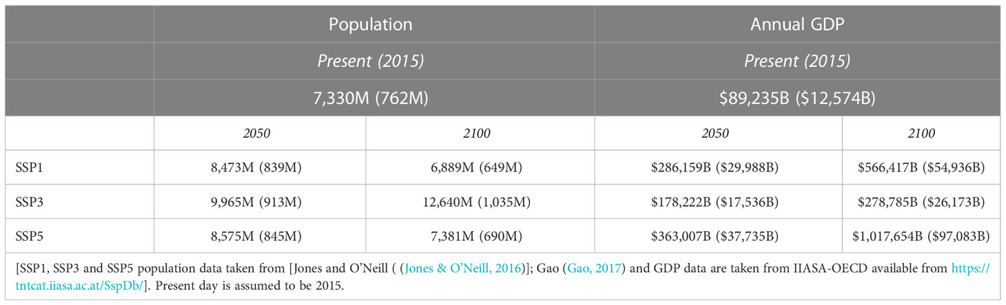
Table 1 Global and Low Elevation Coastal Zone (shown in parentheses) population and GDP estimations (Billions of US$ in 2005 currency) for various Shared Socio-economic Pathway (SSP) narratives.
The magnitude and duration of coastal flooding depends not only on the magnitudes of these major processes but on the interactions between them, and how they may change in magnitude over time. For instance, all of these processes may change in the future due to climate change. Coastal flooding may result from the overflow of coastal defences or by wave overtopping, or both. Once overtopped, the extent of flooding will depend on both the duration of the event and the topography being flooded. In addition, whilst non-linear interactions between the major processes (tide, surge, waves) may exacerbate the ultimate flooding magnitude, the hydrodynamic processes related to surface roughness may attenuate water levels (Vafeidis et al., 2019). As storm-induced extremes are often associated with heavy rain, compound impacts from river flooding and coastal innundation may determine the ultimate flooding extent. Reviews highlighting such complex interactions can be found in Idier et al. (2019) and Haigh et al. (2019).
In order to assess the projected impacts of changes in ESL over the next century, it is necessary to estimate (i) global magnitudes of coastal flooding during extreme events, (ii) the levels of coastal defences which are already in place and may be developed in the future, (iii) the probability of damage to assets and (iv) populations at risk. In addition, such an analysis needs to consider both how populations and gross domestic product (GDP) may change in the future (Shared Socio-economic Pathways, SSPs) (O’Neill et al., 2014), and also projected changes to greenhouse gas levels (Representative Concentration Pathways, RCPs) (Church et al., 2013; Oppenheimer et al., 2019). As all these quantities vary spatially, such an analysis needs to be regional by nature, aggregating results to the global scale.
Analyses addressing the impacts of projected coastal flooding at the national (Antunes et al., 2019; Fang et al., 2020; Haigh et al., 2020), continental (Reguero et al., 2015; Abadie et al., 2016; Hauer et al., 2016; Vousdoukas et al., 2018b) and global levels (Hinkel et al., 2014; Kirezci et al., 2020; Tiggeloven et al., 2020; Hunter et al., 2017; Lincke and Hinkel, 2018; Nicholls et al., 2018) within a coastal flood risk framework are important planning tools (Schinko et al., 2020; Tiggeloven et al., 2020; Vousdoukas et al., 2020). This study undertakes such a detailed analysis for countries and regions globally, estimating values of both Expected Annual Population Affected (EAPA) and Expected Annual Damage (EAD) (Hinkel et al., 2014; Vousdoukas et al., 2020). These quantities represent important measures of the socioeconomic impacts of coastal flooding.
The study builds on previous analyses and includes values of projections of regional sea level rise from the IPCC SROCC (Intergovernmental Panel on Climate Change, Special Report on the Ocean and Cryosphere in a Changing Climate) (Oppenheimer et al., 2019). The results are provided at the global, regional and national levels. As such, the outcomes of this study are intended to be a resource for policy developers considering the impacts of projected coastal flooding and the mitigation and adaptation measures which may be required for flood risk reduction in the coastal zone.
The present analysis builds on the study of Kirezci et al. (2020) which estimated coastal flood exposure for a 1 in 100-year event at each of a total of 9,864 segments along global coastlines. Kirezci et al. (2020) adopted the Multi-Error Removed Improved-Terrain (MERIT) digital elevation model (Yamazaki et al., 2017) and assumed no coastal flood protection was in place. At each of these coastal segments, we consider existing coastal defences reported in the Dynamic Interactive Vulnerability Assessment database (DIVA) (Hinkel and Klein, 2009). The coastal flood defence levels are estimated from national policies, expressed as return period design values (see Materials and Methods). Based on the calculated probability distribution function of coastal flooding at each location and a depth-damage relationship (Hinkel et al., 2014) (see Materials and Methods), the EAPA and EAD (Zhou et al., 2012; Hinkel et al., 2014) are calculated for each region/nation, both for the present day and a range of future scenarios. The inclusion of a depth-damage relationship means that actual damage can be estimated, rather than simply determining the full value of assets exposed to damage by flooding (Kirezci et al., 2020). The calculation of EAPA and EAD requires an extension of the analysis to probabilities other than the 1 in 100-year event presented by Kirezci et al. (2020) and the integration over all such possible extreme events (Materials and Methods).
The calculation of EAPA and EAD requires gridded projections of gross domestic product (GDP) and population, from which exposed population and assets can be estimated (Hallegatte et al., 2013; Hinkel et al., 2014). In order to guide climate change studies, a set of reference pathways describing plausible alternative trends in the evolution of society and ecosystems over the coming century are available in the form of Shared Socioeconomic Pathways (SSPs) (O’Neill et al., 2014). Global gridded values of population are available for these SSPs (Jones and O’Neill, 2016; Gao, 2017). The SSPs can be combined with radiative concentration pathways RCP2.6, RCP4.5 and RCP8.5 to define plausible futures for the Earth. Four scenario combinations have been considered in this study: ‘Sustainable world’ (RCP2.6 and RCP4.5 combined with SSP1; SSP1-2.6 and SSP1-4.5); ‘Fragmented world’ (RCP8.5 and SSP3, SSP3-8.5) and ‘Fossil-fuel based world’ (RCP8.5 and SSP5, SSP5-8.5). The SSP1-2.6 combination is considered because of wide precedence in Coupled Model Intercomparison Project - 6 (CMIP6) applications as the Paris Agreement (O'Neill et al., 2020; Fyfe et al., 2021). The other three RCP-SSP combinations are widely considered cases for possible higher radiative forcing pathways (van Vuuren and Carter, 2014). Note that there are numerous other RCP-SSP combinations which could have been considered in this analysis. The present cases are believed to provide plausible upper and lower bounds for the future.
The aggregated global population and GDP for the present, 2050 and 2100, are shown in Table 1. For both SSP1 and SSP5 the global population increases by 2050 before declining by 2100. In contrast, the global population continues to grow for SSP3. All three SSPs show a continually increasing global GDP, with SSP5 resulting in the most rapid increase and SSP3 the slowest. It should be noted that the various SSPs show rather different trajectories in the developed and developing worlds. Hence, the global trends shown in Table 1 are not equally reflected in all regions of the world.
At both 2050 and 2100, values of EAPA and EAD at any location will be impacted by: the ESL hazard, determined here for each of RCP2.6, 4.5 and 8.5; the population and GDP exposure, determined by the SSP and the height of coastal defences, which is determined by the adaptation scenario adopted. The analysis considers all of these variables in terms of the following three scenario combinations. Initially, we consider a “baseline case” where population, GDP and adaptation levels remain constant at values for the baseline year (here taken as 2015) and only the ESL varies for each of RCP2.6, 4.5 and 8.5 (no socio-economic change). Although this is not a plausible future case, it provides a means of determining how much of the calculated EAPA and EAD is attributable to future changes in ESL and how much is attributable to population and GDP change. In addition, two adaptation scenarios are considered for each RCP/SSP combination. The first adaptation scenario (adaptation matching ESL change), assumes that society responds to future sea level rise by introducing adaptation in the form of raising existing and building new defences, such that the height of enhanced coastal protection matches the increase in ESL. In the second adaptation scenario, no additional adaptation measures to respond to increased flooding are introduced; current defences are maintained but not upgraded and no new defences constructed (no additional adaptation). This describes an implausible future, as societies have a long history of adapting to sea level rise and will continue to do so by either raising defences or retreating from the coast (Oppenheimer et al., 2019; Hinkel et al., 2021). Nevertheless, it is standard practice to consider no adaptation in order to illustrate the magnitude of adaptation needs (Oppenheimer et al., 2019).
As described below, the present analysis uses a large number of datasets (see Data Section) and calculates a range of quantities from these data (see Figure 1). As a guide to the reader, a glossary of terms and acronyms is included in Supplementary Material (see Glossary for the Abbreviations Used in the Manuscript).
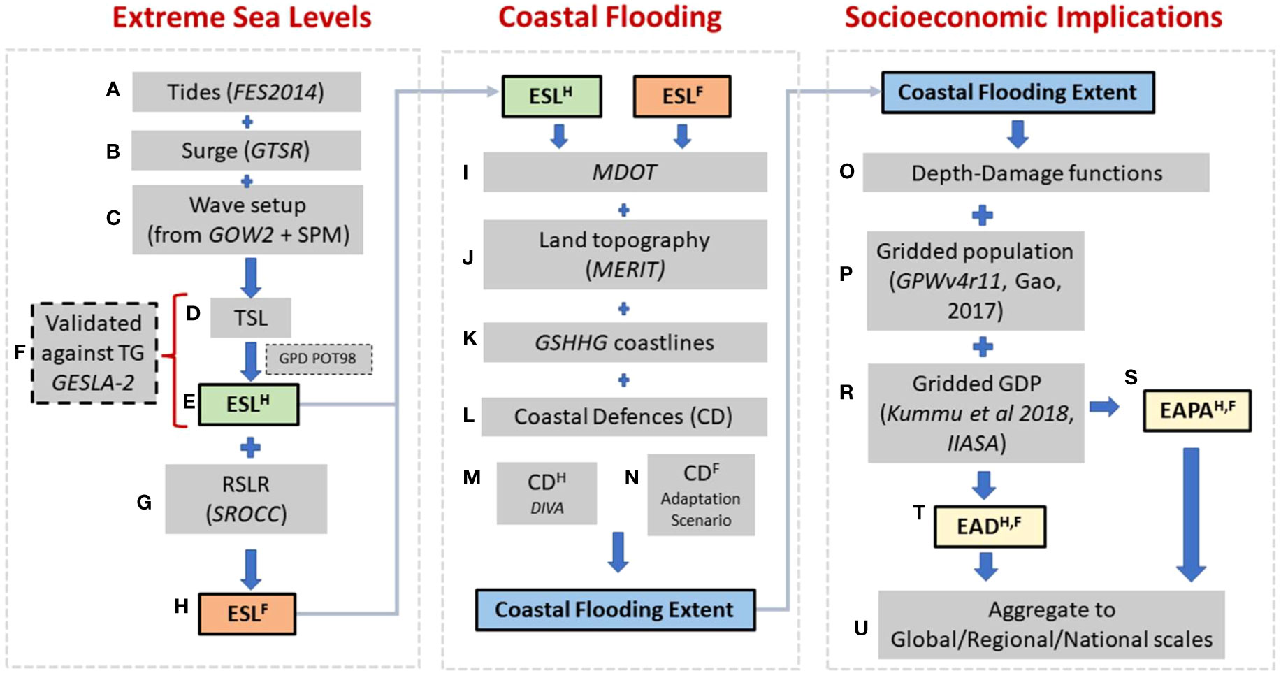
Figure 1 Diagrammatic representation of the processes used in the determination of the Socioeconomic Impacts of projected extreme coastal flooding. As explained in the Materials and Methods section, the full analysis involves a large number of sequential steps, divided into three broad areas. Initially, Extreme Sea Levels (ESL) are determined for a variety of probabilities of exceedance at coastal segments (DIVA) around the world. These are determined both for the historical period (superscript H) and future periods (superscript F). These values of ESL are then used to determine the extent of Coastal Flooding, accounting for existing and future Coastal Defences (CD). Finally, we sum over all exceedance probabilities to determine the Expected Annual People Affected (EAPA) and Expected Annual Damage (EAD). The analysis uses numerous global datasets (shown in italics). Terms and abbreviations are defined in “Materials and Methods” section, where each step is referred to an element in the figure defined by the alphabetical reference (A–U).
Materials and methods
The present analysis can be divided into three broad sequential categories, shown diagrammatically in Figure 1. These include the estimation of: (i) Extreme Sea Levels (ESL) for a range of probabilities of exceedance, both for the historical period (1979-2014) (referred to as present day, 2015) and the future (2050 and 2100), (ii) Coastal Flooding Extent for these ESLs; both historically and in the future with coastal defences representing a range of defined adaptation scenarios and (iii) Socioeconomic Implications in terms of EAPA and EAD for each adaptation scenario and SSP aggregated globally, regionally and nationally.
The global-scale, but regional-resolution, analysis described below requires several simplifying assumptions in calculating ESL and flooding extent. These assumptions may result in imperfections at specific coastal locations (see Limitations Section), however, they are necessary to construct a tractable solution at global scale.
Extreme sea levels
Extreme sea levels were calculated globally for each DIVA coastal segment using the approach described by Kirezci et al. (2020) and shown diagrammatically in Figure 1. Time series (with a 10-minute time base) of the historical total sea level [TSL(t)] were defined at each DIVA segment as the linear summation of tide (T), storm surge (S) and breaking wave set-up (W) (Figures 1A–D). Global values of each component of the TSL were determined from the following global datasets – tide [FES2014, (Carrere et al., 2015)], storm surge [GTSR, (Muis et al., 2016)] and breaking wave set-up [GOW2, (Perez et al., 2017)]. The calculation of TSL values using the linear summation of T+S+W is a significant simplification of the complex physics of coastal flooding (see Limitations Section), however, this simplistic approach has been validated by Kirezci et al. (2020) against an extensive database of tide gauge data, GESLA-2 (Woodworth et al., 2017), for both ambient conditions and upper percentiles (Figure 1F) (see Kirezci et al., 2020, their Figures S2, S3, S7 and Tables S1, S2 and Limitations Section, below).
Values of Extreme Sea Levels, ESLHn, can be determined from TSL values using Extreme Value Analysis (EVA). Here, the superscript “H” indicates that the value of extreme sea level is associated with the historical period, with “n” denoting the return period of the extreme sea level. The return period is related to the probability of exceedance (probability of event occurring in any one year), “p”, by p=1/n. Kirezci et al. (2020) compared a range of EVA approaches with tide gauge data and concluded that a peaks-over-threshold analysis with a probability distribution defined by the Generalized Pareto Distribution (GPD) (Figure 1E) using a 98th percentile threshold produced results with the smallest bias for ESLHn. In the present analysis, return period values of ESL, i.e., ESLHn, were determined with n = 1, 10, 100, 1000, 10000 years at each coastal location.
The projected future extreme sea levels (ESLFn) (Figure 1H) for 2050 and 2100, were determined by the addition of the relative sea level rise due to climate change (RSLR) to ESLHn (Figure 1G). Here, the superscript “F” denotes the future values of extreme sea level (i.e. RSLR included). This was again calculated at each coastal location defined by the DIVA segments with RSLR varying regionally and defined on a global grid (Church et al., 2013). In contrast to Kirezci et al. (2020), who used AR5 projections of RSLR (Church et al., 2013), the present study uses the more recent IPCC SROCC RSLR projections (Oppenheimer et al., 2019). The approach where ESLF>n=ESLHn+RSLR assumes that changes of tide, storm surge and breaking wave setup over the future projected periods are small compared to RSLR. Kirezci et al. (2020) considered this issue in detail and concluded the errors, at global scale, are small compared to uncertainties in the estimation of TSL, RSLR and the EVA statistical uncertainty. Note, however, that at specific locations there may be significant differences.
Coastal flooding
The extent of coastal flooding is modelled in terms of three major components: the ESL, presence of any coastal protection in-place and the land topography. Once the ESLH,Fn (i.e. ESLHn or ESL,Fn) were determined, as outlined above, the ESL values and the land topography were referenced to the same datum using the Mean Dynamic Ocean Topography (MDOT) (Muis et al., 2017; Kirezci et al., 2020) (i.e. ESLH,Fn+MDOT ) (Figure 1I). The gridded coastal topography was determined from the MERIT digital elevation model (DEM) (Yamazaki et al., 2017) (Figure 1J). An alternative DEM, CoastalDEM (Kulp and Strauss, 2019) was also tested but produced coastal flooding extent which was deemed unrealistically large. Hence, it was not considered further. The datum-corrected ESLH,Fn values were then assigned to areal regions using Thiessen polygons (Kirezci et al., 2020), with the seaward extent defined by the (GSHHG, version 2.3.7, [2017]) (Wessel and Smith, 1996) (Figure 1K).
The levels of any coastal protection at each location were defined using the DIVA database, which estimates protection levels using a stylized model of protection based on local floodplain population density and local GDP per capita (Sadoff et al., 2015), complemented with protection levels for the largest 136 coastal cities of Hallegatte et al. (2013). These values are represented in the DIVA database by the flood probability associated with these protection levels (e.g. 50-year return period protection level) (Figure 1L). The GPD probability distributions were then used at each location to determine the equivalent coastal defence level, CDHx, where “x” is the local protection level return period for that location (Figure 1M). It was assumed that this level of coastal protection was in place at present, at each location. The protection levels in 2050 and 2100 (CDFx) were determined according to the adaptation scenario, i.e., adaptation matching ESL change and no additional adaptation scenarios (Figure 1N). If ESLH,Fn was below the coastal protection value, no coastal flooding occurs in that polygon for a 1 in n-year event. Once ESLH,Fn exceeded the protection level, the protection was assumed to be overtopped, and the flooding depth was now set by ESLH,Fn and the topography. Note that the DIVA dataset described above sets the protection level for the Netherlands at a 1 in 5,000-year event and for Belgium at variable levels between 1 in 50 and 1 in 100-year events. These values appear inconsistent with present practice in both nations and hence we have adopted 1 in 10,000-years for the Netherlands and 1 in 1,000-years for Belgium.
The coastal flooding extent at each location was calculated using a “bathtub” approximation (Figure 1J) and the MERIT DEM, which has 3 arcsecond (~90 meter) horizontal resolution. There was also a requirement that the location was shore-connected (Kirezci et al., 2020). As a result, coastal flooding extent can be determined for each ESLH,Fn return period, i.e., n =1, 10, 100, 1000, 10000 years. The flooding extent was determined at 1 km resolution, in order to be computationally consistent with all the gridded datasets used in this study.
The representation of coastal protection outlined here is consistent with the construction of coastal dykes or barriers and our assumption of a “bathtub” flooding model. It has been used in a number of previous studies (Hinkel et al., 2014; Muis et al., 2016; Vousdoukas et al., 2018b; Tamura et al., 2019). An alternative characterization of protection level would be that the protection is provided by policies which require all structures to be elevated to the protection level. This may be an option for new construction but not historical developments. In such a representation, the flooding extent can be represented by adopting ESLHx as the new elevation datum and measuring flooding depth above this protection elevation.
Socioeconomic implications (expected annual damage and expected annual people affected)
Knowing the depth of flooding and the value of assets in an area does not provide a direct measure of the resulting damage. Such an understanding can, however, be obtained by adopting a depth-damage function (Messner et al., 2007; Hinkel et al., 2014) (Figure 1O) which defines the percentage of the value of the assets damaged as a function of flood depth. Following Hinkel et al. (2014), such functions generally have a declining slope, indicating that additional damage decreases with flooding depth, with a common form given by (Messner et al., 2007; Hinkel et al., 2014)
where V is the proportion of the assets damaged and d is the water depth at the location of interest for ESLHn or ESLFn (Figures 1E, H). Equation (1) indicates that at a water depth of 1m, 50% of the value of the assets are lost.
As events of all probabilities can occur in any year, to determine the EAPA or EAD (Figures 1S, T) it is necessary to sum over all probabilities of exceedance (return periods) (Meyer et al., 2009; Zhou et al., 2012; Hinkel et al., 2014; Muis et al., 2015). The computational steps to achieve this for the discrete gridded data are as follows:
• The flooded areas for each return period (n = 1, 10, 100, 1000 and 10000) were calculated.
• The flood depths, d (ESL minus land elevation) for the flooded areas were calculated at each computational cell. This process also accounts for coastal defences in place, as outlined above.
• The depth-damage function, V , as in Eq. (1) was calculated for each computational cell. Note that d is a function of return period and coastal defences in place (adaptation scenario).
• The value of the assets exposed to flooding can be estimated from the relationship, A=2.8×POP×GDPPC (Hallegatte et al., 2013; Hinkel et al., 2014), where A is the value of the assets exposed in US$, POP is the population and GDPPC is the Gross Domestic Produce per capita (US$).
• The damage (US$) at each gid cell can then be determined as D>AM=A*V. For the present day (2015), the POP was taken from the data of Gridded Population of the World (GPWv4) (Center for International Earth Science Information Network (CIESIN), 2018) and for years 2050 and 2100 and SSP1, SSP3 and SSP5 narratives from the gridded data of Gao (2017) (Figure 1P), which is an enhanced version of the data proposed by Jones and O’Neill (2016). The GDP data for the present day (2015) were obtained from (Kummu et al., 2018) and for future times and SSP narratives from the IIASA database (Riahi et al., 2017) (https://tntcat.iiasa.ac.at/SspDb/) (Figure 1R).
• This process was repeated for each probability of exceedance, p , considered (i.e. Return periods, n =1, 10, 100, 1000, 10000 years). This results in DAM vs p and POP vs p curves at each grid cell.
• The EAD and EAPA can been determined by finding areas under these DAM vs p and POP vs p curves (Meyer et al., 2009; Muis et al., 2015; Tiggeloven et al., 2020). This was achieved using a trapezoidal approximation to the discrete values of p
• The values were then summed over the grid cells and aggregated at global, regional and national levels (Figure 1U).
The approach adopted above (Meyer et al., 2009; Muis et al., 2015; Tiggeloven et al., 2020) is equivalent to that of Hinkel et al. (2014) but implemented in a different manner. Hinkel et al. (2014) first produce continuous functions of cumulative exposure below a given contour and then compute the expectation using the continuous formula for mathematical expectation. To calculate EAD (or similarly EAPA), they then integrate twice: first analytically over the derivative of the cumulative elevation (multiplied by the depth-damage function) and then numerically over the exceedance probability. The second integral is similar to the summation above for the discrete values of probability of exceedance. The discrete cell-based approach used here, facilitates the combination of the many gridded datasets used and is readily applied at global scale.
Confidence limits
The estimated values of ESLH,Fn are statistical quantities obtained from the GPD fit to the model data and extrapolated to the desired probability level, n . In addition, the values of RSLR contain statistical uncertainty. Confidence limits for the values of ESLH,Fn at each coastal segment were calculated using a bootstrap approach (Efron, 1979; Meucci et al., 2018) in which 1000 realizations of the ESL were generated at each DIVA point (Kirezci et al., 2020). For ESLFn, the uncertainty range for RSLR is also included. From this analysis 90th percentile confidence limits were calculated for ESL and subsequent quantities, which are determined from these values (e.g. EAPA and EAD). Therefore, the confidence limits were determined at each probability level considered and the results aggregated through the discrete steps described above for the determination of EAPA and EAD. Tables 2, S1-S3 reflect these confidence intervals together with mean values.
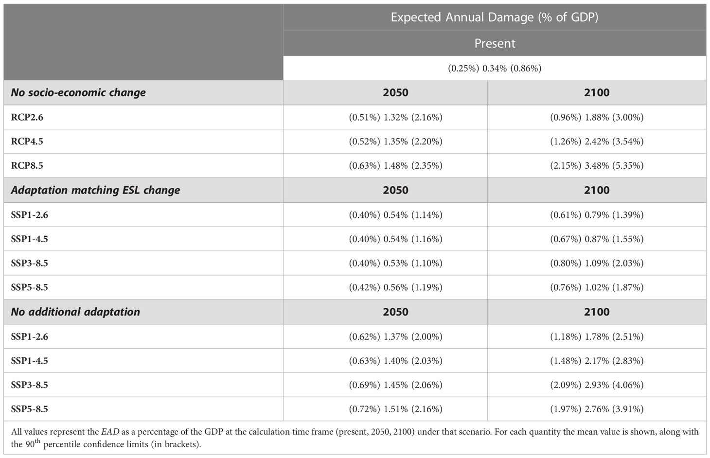
Table 2 Expected Annual Damage (EAD) for the present (2015), 2050 and 2100 for the scenarios of: no socio-economic change, adaptation matching ESL change and no additional adaptation and different RCP/SSP pathways/narratives.
The confidence limits described above are a result of the statistical variability inherent in the extreme value analysis and do not include potential errors in the datasets or as a result of the approximations necessary to form the global solutions, as outlined in the Limitations Section.
The summations to determine EAPA and EAD (see Socioeconomic Implications Section) involve considering all possible return periods. To approximate this, we consider events as rare as 1 in 10,000 years (p=10-4). For such events the confidence limits for flood areas become large. However, as the values of probability are so small, they make only a small contribution to the estimated values of EAPA and EAD. As such, the potential errors do not become excessively large.
Data
As described in the “Materials and Methods” section above, the present analysis integrates a broad range of global datasets. These datasets are described below using the same three groupings of (i) Extreme Sea Levels, (ii) Coastal flooding and (iii) Socioeconomic implications (i.e., EAPA and EAD).
Extreme sea level analysis
Tide levels
The global tidal elevations were taken from FES2014 (Lyard et al., 2021; https://www.aviso.altimetry.fr/en/data/products/auxiliary-products/global-tide-fes/description-fes2014.html) which is a finite element hydrodynamic model solving the tidal barotropic equations and assimilating in-situ tide gauge and altimeter data. The dataset has a spatial resolution of 1/16° (Figure 1A).
Storm surge
The global storm surge levels were taken from the Global Tide and Surge Reanalysis (GTSR) dataset (Muis et al., 2016). This dataset was generated using Delft3D FM, with a spatial resolution ranging from 50 km in the deep ocean to 5 km in coastal areas, forced with ERA-Interim (Dee et al., 2011) atmospheric parameters. The GTSR surge timeseries data were then downscaled to 10 minutes temporal resolution over the period of 1979-2014 (36 years) (Figure 1B).
Wave setup
To determine the contributions from waves to the time averaged sea level, the GOW2 wave dataset (Perez et al., 2017) was used. Wave setup was defined using the SPM (US Army Corps of Engineers, 1984) method, with a constant assumed bed slope of 1/30 globally. A detailed analysis was conducted by (Kirezci et al., 2020), where two other bed slopes (1/15 and 1/100) were tested. To investigate uncertainty due to different wave setup methodologies, an alternative method suggested by (Stockdon et al., 2006) was also considered, with a 1/30 bed slope. It was concluded that, for ESLH100 , there is a negligible difference between the two methods at the global scale (Kirezci et al., 2020) (Figure 1C).
Regional relative sea level rise
To account for future projections of regional relative sea level rise, two global datasets were used, i.e., SROCC (Oppenheimer et al., 2019) and AR5 (Church et al., 2013) for RCPs 2.6, 4.5 and 8.5. Note that, an analysis with AR5 was conducted in order to compare the present study with previous computations. The major difference between RSLR projections from AR5 and SROCC is that the SROCC RSLR dataset includes more recent projections of Antarctic Ice Sheet (AIS) contribution to RSLR. This is discussed in detail by Oppenheimer et al. (2019) (Figure 1G).
By 2050, the global mean SLR projections are generally consistent between the published AR5, SROCC and AR6 values, irrespective of the RCPs. By 2100, however, global mean SLR projections show lower agreement among both the RCPs and the published global mean SLR projections. This is mainly due to the projected ice-sheet contribution. Although that is the case, AR6 (Figure 9.25 therein) shows that the global mean SLR projections are consistent among the RCPs.
Tide gauge data
A quasi-global tide gauge observation dataset, GESLA2 (Woodworth et al., 2017), was used to estimate ESLH100 from the recorded timeseries and thus validate estimated Extreme Sea Levels calculated from the reanalysis timeseries (T+S+W) (Figure 1F).
Coastal inundation extent
Mean sea level datum
The datum for the historical timeseries, hence ESLs, is referenced to MSL. To bring the land topography and the ESLs to the same reference level, the Mean Dynamic Ocean Topography (Rio et al., 2014) was used. This is the difference between the time-averaged sea surface and the geoid reference line (Figure 1I).
Land topography
Coastal land elevations were taken from the MERIT Digital Elevation Model (DEM) (Yamazaki et al., 2017). The MERIT DEM (Yamazaki et al., 2017) was developed from existing spaceborne DEMs [SRTM3 v2.1 and AW3D-30m v1 (Farr et al., 2007); Jarvis et al., 2008] by eliminating major error components from the existing DEMs, covering land areas from 900N-600S. MERIT DEM has 3 arcsecond (~90 meter) horizontal resolution and has a vertical datum of EGM96 (https://cddis.nasa.gov/926/egm96/egm96.html) (Figure 1J).
Coastline data
The GSHHG dataset (Wessel and Smith, 1996) was used to define the global coastline for calculations of coastal flooding extent. The dataset was used to bring a variety of the global data layers to a consistent coastline position (Figure 1K). Note that no attempt is made to define the change in position of the coastline, as a result of RSLR (see Extreme Sea Level Analysis Section) in 2050 or 2100. This is not necessary as all changes in population and GDP are defined for gridded locations and not referenced to the GSHHG coastline (see Socioeconomic Implications Section).
Coastal defences
The global coastal defences dataset is taken from the DIVA database (Vafeidis et al., 2008; Hinkel et al., 2014), where the defence levels are defined as return period values of extreme sea level (e.g. 50-year return period protection level) at each DIVA segment. Here, we estimate the flood elevation of these return values (in metres) from an assumed GPD extreme value probability distribution function at each coastal location (See “Materials and Methods”) (Figures 1M, S5).
Socioeconomic implications
Population
Two global gridded population datasets were used to account for the present and future projections of population. For the present case (2015), the NASA Socioeconomic Data and Applications Center (SEDAC) GPWv4 Rev. 11 database (https://sedac.ciesin.columbia.edu/data/set/gpw-v4-population-count-rev11) of population count from the 2015 census data (30 arc sec., ~1 km at the equator, resolution) was used. To account for the population changes by 2050 and 2100, the gridded population data of Gao (2017), with 1km resolution, was used for SSP narratives SSP1, SSP3 and SSP5 (Figure 1P).
Gross domestic product
Similar to the population data, GDP estimates were considered for both the present and future projections. The GDP data for the present case (2015), were taken from Kummu et al. (2018), which consists of GDP per capita (PPP) data on a 5-arc min grid (downscaled to 30 arc-sec to be consistent with the other datasets). For the future changes of GDP, the global GDP data were obtained from IIASA (Riahi et al., 2017) (https://tntcat.iiasa.ac.at/SspDb/) for each SSP case (Figure 1R). Note that, the projected values of GDP, were not given in gridded format, they were rather given on a national scale. The GDP at each country was distributed at the same proportion of the population density (Gao, 2017) for each grid. To be consistent among the datasets, all the $US values are given for the year 2005.
Results
As outlined in Materials and Methods, the global-scale, but regional-resolution, analysis undertaken here requires several simplifying assumptions in calculating ESL and flooding extent. These assumptions may result in imperfections at specific coastal locations (see Limitations Section). However, as shown in the extensive validations of Kirezci et al. (2020), when aggregated to regional and global values, the computed ESLs are in good agreement with historical tide gauge data (see Kirezci et al., 2020, their Figures S2, S3, S7 and Tables S1, S2, which shows that over 681 tide gauge locations, the RMS error of the TSL is less than 0.2m at 75% of locations). As a result, in the present analysis, results are not presented at individual coastal segments. Rather, results are presented as figures and tables showing values aggregated into 51 Climate Reference Regions (Iturbide et al., 2020) and as tables at the national level (see SM; Note on National Level EAPA and EAD Analysis).
Below, results are presented at both the Global and Regional/National scales. Within each of these sections, we consider the case of no socio-economic change and the scenarios of adaptation matching ESL change and no additional adaptation. Table 2 shows all the combinations of adaptation scenario, SSP/RCP and future time considered. For the baseline no socio-economic change case, variations in EAPA and EAD result only from changes in ESL, with no future adaptation, and hence the results demonstrate only the impacts associated with climate related sea level rise scenarios (here, RCP 2.6, 4.5 and 8.5). For the adaptation matching ESL change and no additional adaptation scenarios, impacts are a result of changes in population, GDP and ESL. Therefore, each SSP and RCP combination described here is considered for both adaptation scenarios. Note that, because of space limitations, only the global results for RCP 4.5 (i.e. no Regional/National scale) are presented here (and in SM), as these results almost always fall between the other scenario combinations.
Global scale results
The global values of present and projected future population and GDP under various SSP narratives are not necessarily representative of coastal regions. Therefore, to provide a representative foundation for our analysis, we first determine the projections of population and GDP for the Low Elevation Coastal Zone (LECZ), defined as the shore-connected area below an elevation of 10 m above mean sea level (McGranahan et al., 2007). These values were determined by summing the gridded population and GDP datasets (Jones and O’Neill, 2016; Gao, 2017; Riahi et al., 2017) below an elevation of 10 m (above MSL) for present day and future SSP narratives. Note that only shore-connected grid cells are counted. As shown in Table 1, at present 762M people reside in the LECZ (10.4% of the global population) generating annually US$12,574B (14.1% of global GDP). These values are comparable (slightly lower) to the results of Jones and O’Neill (2016), the differences likely being due to differences in the elevation datasets used and the geospatial masking adopted. Consistent with the projected global changes (Table 1), the LECZ population and GDP are projected to increase by 2050 for all three SSP narratives. By 2100, however, the LECZ population decreases under SSP1 & SSP5, but continues to increase under SSP3. The percentage of both the global population in LECZ regions and GDP generated in these regions in both 2050 and 2100 is, however, projected to remain comparable to the present day (decreases for all SSPs by less than 1%). Note that the “present” (baseline period) population and GDP are based on 2015 values. Hence, it is observed that (Table 1), the relative importance of the LECZ in terms of percentage of global population and GDP generated is not projected to change significantly over the 21st century. It should be noted that MacManus et al. (2021) indicate that in recent years there is evidence that population growth rates in LECZs are higher than those outside these regions due to urbanization. The results above indicate that this trend is not projected to continue in the future.
As shown in Table S1 (Supplementary Material), the analysis applied here shows that for present day (2015) ESL, mean EAPA (by flooding) is 34M (30M – 61M) people, where the range shown in brackets is the 90% confidence interval (see “Materials and Methods”). Similarly, the present day mean global EAD is $307B ($220B - $767B), where all values are in 2005 US dollars (see “Materials and Methods” and “Data” sections). The EAD is significantly lower than the value of assets exposed to the 100-year flooding event reported by Kirezci et al. (2020), because the EAD are estimates of actual damage to assets rather than the value of assets exposed to flooding. As such, EAD is a metric that integrates over all return periods (not just the 100-year event), also considering the differential damage to assets at different elevation level via depth-damage functions (see “Materials and Methods”).
No socio-economic change case
As noted above, under the no socio-economic change case, it is assumed that there are no changes in population, GDP or future adaptation, but ESL probabilities, and hence the flood risk, change for emission representative concentration pathways, RCP2.6, 4.5 and RCP8.5. The resulting global increases in values of EAPA and EAD in 2050 and 2100 are shown in Table S1. By 2100 for RCP2.6 the EAPA changes by +78M people (total EAPA is 329% of the present value) and for RCP8.5, EAPA changes by +146M people compared to the present day (529% of present value). Similarly, by 2100, EAD changes by +$1,366B (545% of present value) for RCP2.6 and by +$2,795B (1010% of present value) for RCP8.5. Note, for clarity, throughout this paper increases (or decreases) are shown with a “+” (“-”) sign whereas absolute totals have no sign. Also, all such change values are relative to the baseline year 2015. The percentage values in parenthesis show the changes in the absolute values compared to present day (Absolute Future Estimate/Present Value x 100).
Adaptation matching ESL change scenario
The impact due to the projected ESL, population and GDP changes for the adaptation matching ESL change scenario, as defined by the various RCP and SSP narratives, is shown in Table S2. Under the SSP1 narrative, both the global and LECZ populations increase by 2050 and then decrease by 2100 (relative to 2015). The mean EAPA shows a similar behavior for SSP1-2.6, increasing by +15M people by 2050 but by only +11M people by 2100 (both figures relative to the present-day, 2015; confidence limit changes relative to present also shown in Table S2). With the SSP3 narrative, the global and LECZ populations increase continually through the 21st century, which are also reflected in the EAPA for SSP3-8.5 (Table S2), with a change of +30M people affected by 2050 and +85M people affected by 2100. The changes in global and LECZ populations for SSP5 (Table 1) are similar to SSP1, increasing in 2050 and subsequently decreasing by 2100. However, due to the impact of increasing ESL over the century, the projected EAPA for SSP5-8.5 continually increases by +17M by 2050 and +25M by 2100 (both relative to 2015).
The EAD is a function of both population and GDP, (and vulnerability) and hence its projected changes under this scenario are more complex than that of the EAPA. Unlike population, the global GDP is projected to continually increase over the 21st century for all SSPs. The largest growth is projected for SSP5 and the smallest for SSP3. In response, there is a continual growth in EAD for all cases considered. The largest changes both at 2050 and 2100 are seen for SSP5-8.5 (Table S2), +US$1,739B by 2050 and +US$10,120B by 2100. This reflects the projected high level of growth in GDP which overwhelms the relatively small population decreases (compared to the baseline year 2015) projected in coastal regions.
No additional adaptation scenario
Table S3 shows the results for the no additional adaptation scenario, where defence levels remain unchanged at present-day levels but there are changes in population, GDP and ESL, and hence flooding extent as a function of time. In this case, for all SSP narratives, the EAPA increases by both 2050 and 2100 compared to present values (2015). This occurs because, even if the population densities decrease, as is the case under SSP1 and SSP5, the area flooded continues to increase. However, the balance between population decrease and flood extent increase is such that the increase in EAPA for SSP1-2.6 in 2050 (+63M) is larger than by 2100 (+57M). By 2100, most people are impacted under the SSP3-8.5 pathway with a change of +212M people (724% of present value). In terms of EAD, there is a continual increase with time across all SSPs. By 2100, the SSP3-8.5 pathway shows the lowest change in EAD at +US$7,858B (2660% of present value), reflecting the low GDP growth for this narrative. In contrast, the SSP5-8.5 pathway shows the largest change in EAD of +US$27,736B (9135% of present value), again as a result of the large growth in GDP for this narrative.
A comparison of the no socio-economic change case and the no additional adaptation scenario shows the impact of projected changes in population and GDP on values of EAPA and EAD. Note that, both scenarios assume no future adaptation. By 2050, changes in socioeconomic development have a larger impact than the effects of ESL changes alone, whilst this outcome reverses by 2100 under SSP1 and SSP5 narratives, except SSP3-8.5 (compare all RCPs in Table 1 with SSP combinations in Table 3). This is due to faster population increase under the SSP3 narrative by 2100. For EAD, a more straightforward comparison can be made between the two scenarios. The impacts of the projected socioeconomic changes considered in the no additional adaptation scenario on EAD are consistently larger than the no socio-economic change case. By 2100, projected socioeconomic changes result in an almost 10 times larger value of EAD than that of ESL impacts alone (compare RCP8.5 in Table 1 with SSP5-8.5 in Table 3). This result clearly shows the importance of considering projected changes in all three quantities: extreme sea levels, population and GDP, when assessing the impact of episodic coastal flooding in the future.
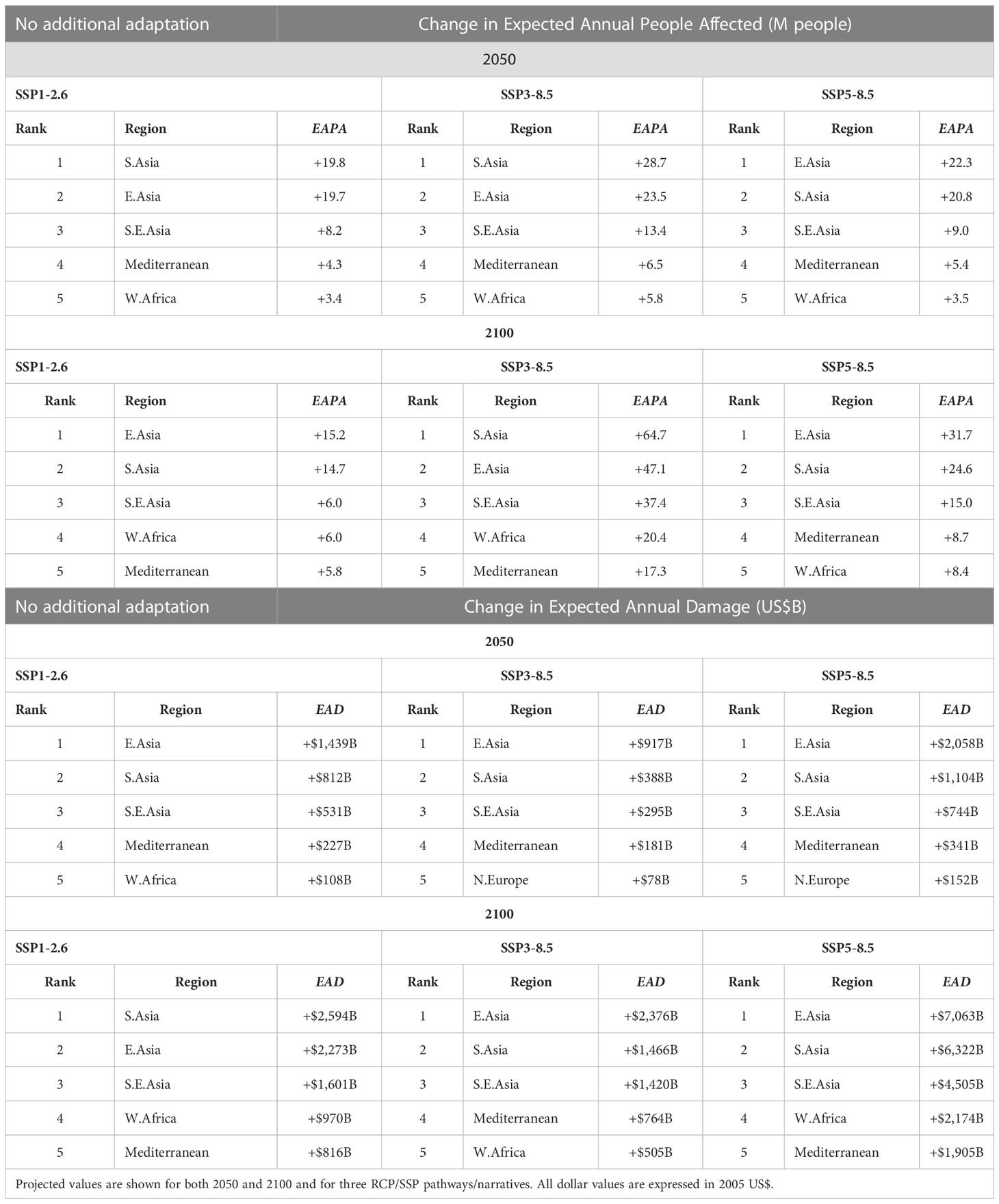
Table 3 Regional ranking of changes in EAPA and EAD relative to 2015 for the scenario of no additional adaptation [assumes that the flooding extent increases in the future with no changes in coastal defences and that population and GDP change with time].
Table 2 shows the values of EAD expressed as percentages of the total produced GDP at the date considered for each RCP/SSP combination (note – total values, not changes). At present, the global EAD is 0.34% of GDP. In the absence of a future increase in adaptation measures (no additional adaptation scenario), this value is estimated to increase to approximately 1.37% - 1.51% by 2050 irrespective of the SSP narrative, reflecting that LECZ population and GDP values do not diverge greatly under any of the SSP narratives by the mid-century. By 2100, however, the largest percentage EAD occurs under SSP3-8.5 with a value of 2.93% of GDP. This is because, although it has the lowest increase in the global GDP, the highest increase in both the population and flooding extent considered in this study is for this RCP/SSP combination. Keeping the socio-economic development constant (no socio-economic change case) results in highest EAD expressed as a percentage of GDP for all SSPs (1.88% – 3.48%) whilst enhancing adaptation measures to match increases in ESL (adaptation matching ESL change scenario), result in the lowest percentage for all SSPs (0.79%-1.09% by 2100).
Hence, ensuring that global levels of flood protection keep pace with projected increases in coastal flooding is projected to decrease the globally averaged EAD as a percentage of GDP by more than half; even for the case of a “fragmented world” (SSP3-8.5), (see Table 2 – 1.09% compared with 2.93%); compared to the case of taking no additional action.
Regional analysis
To discretize the above global scale assessment into regional and national scales, the values at the coastal segments were aggregated into the climate reference regions presented by Iturbide et al. (2020). Figure 2 shows the mean EAPA and EAD for 2015 across these regions. The regions are ranked in terms of these quantities in Table S4. As shown in Figure 2, S. Asia, S.E Asia, E. Asia and W. Africa dominate global EAPA. This occurs because of relatively low levels of coastal defences (<0.5m – Figure S5), large populations and, in the cases of E. Asia and S. Asia, relatively large flooded areas (Kirezci et al., 2020). In total, 79% of the global EAPA is collectively borne by S. Asia (35%), S.E. Asia (34%) and E. Asia (10%), accounting for a total of 27M people impacted annually. Note that the global total EAPA is 34M people (Table S1), demonstrating how these regions dominate the global totals. The EAD shows a similar global distribution for Asia, but with a reduced impact on W. Africa, as a result of the very low GDP of this region. The three highest ranked regions in terms of EAD (2015) contribute 71% of the global total [S.E. Asia (31%), E. Asia (21%) and S. Asia (20%)]. Between them, they account for an EAD of US$219B (Table S4) compared to the global total EAD of US$307B (Table S1). N. Europe, Mediterranean and E.N. America rank 5th to 7th, respectively, largely due to their high GDP. However, these values are still relatively small compared to Asia. For instance, the EAD for S.E. Asia is more than 9 times that of E. N. America.
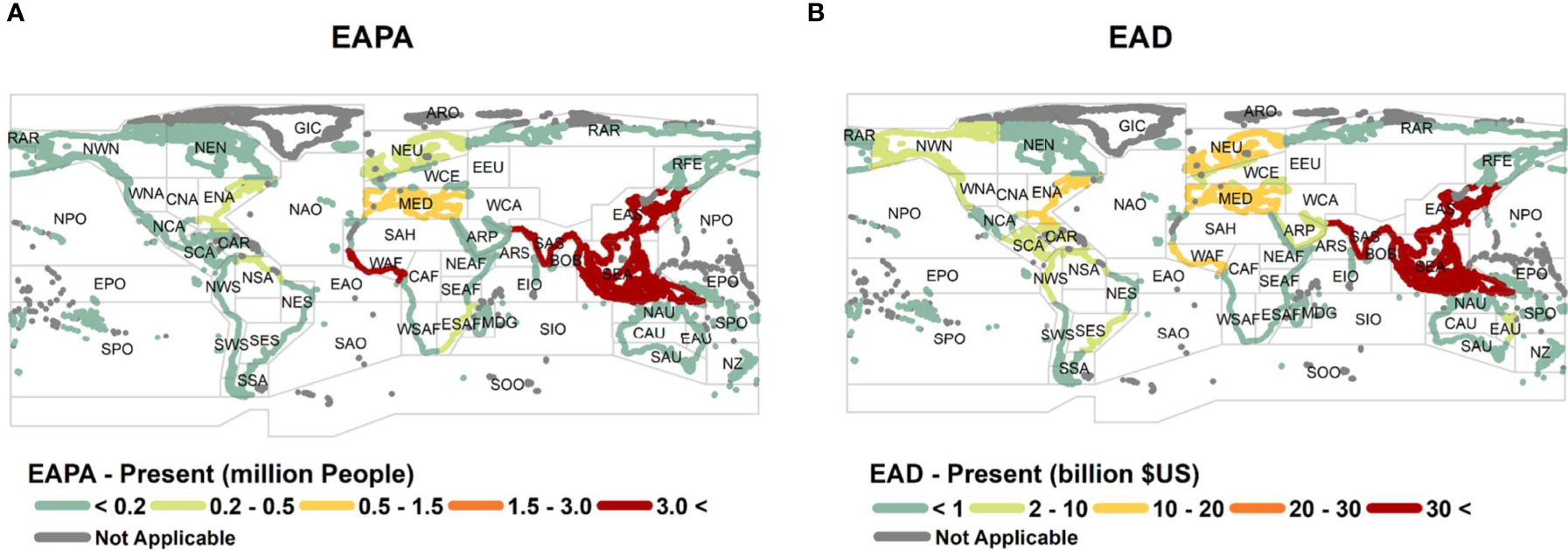
Figure 2 Present-day values (2015) of (A) Expected Annual People Affected (EAPA) and (B) Expected Annual Damage (EAD) in each of the 51 climate reference regions defined by Iturbide et al. (Iturbide et al., 2020).
No socio-economic change case
Under the no socio-economic change case (no changes in population or GDP), E. Asia, S. Asia, S. E. Asia and the Mediterranean (mainly Egypt, also see Tables S9A, B) have the largest increase in EAPA by 2050 (Figure S1 and Table S5A). By 2100, these four regions continue to dominate under both RCP2.6 and 8.5 (Figures S2 and Tables S5A, B). A similar result is obtained for the increase in EAD, however, N. Europe now enters the top five regions by 2100 (Figures S1, S2 and Tables S5C, D). This changed order, compared to the EAPA is because of the relatively high GDP in N. Europe. Note that the Mediterranean values are dominated by Egypt (see national analysis below). By 2100 for RCP8.5, the top three regions (E. Asia, S.E. Asia, and S. Asia) make up 83% of the global EAPA (120/146 – Tables S1 and S5B). Similarly, the EAD for 2100 and RCP 8.5 for the top three regions (E. Asia, S.E. Asia, N. Europe) represent 76% of the global increase in EAD (2,123/2,795 – Tables S1, S5D). That is, for this case where there are no changes in population or GDP, not surprisingly, the percentage increases in EAPA and EAD are similar.
Adaptation matching ESL change scenario
For the adaptation matching ESL change scenario (coastal defence heights are adjusted to respond to the changing ESLs whilst population and GDP also change), in 2050, S. Asia, S.E. Asia and W. Africa show the highest increases in EAPA (Figure S3 and Table S6A) for all SSP narratives. By 2100 (Figure 3 and Table S6B), S. Asia remains the region most impacted in terms of EAPA under all RCP/SSP narratives. Due to rapid population growth, however, W. Africa ranks second for SSP1-2.6 and SSP5-8.5 and third for SSP3-8.5. In 2100, the largest increase in EAD (Figure 3 and Table S6D) occurs for S. Asia followed by S.E. Asia and W. Africa for all SSP narratives. All increases mentioned are relative to 2015 values. One striking impact of the SSP narratives can be seen for S.E. Asia and E. Asia under SSP1-2.6. These rank as the last two regions in terms of EAPA in 2100 (i.e. decreases between -0.5M and -1.1M people – Table S6B) due to projected population decrease for the SSP1 narrative and relatively lower SLR under RCP2.6. However, the projected rapid growth in GDP for these regions means they rank 2nd and the 4th, respectively, for EAD in 2100 under the same RCP/SSP combination (Table S6D).
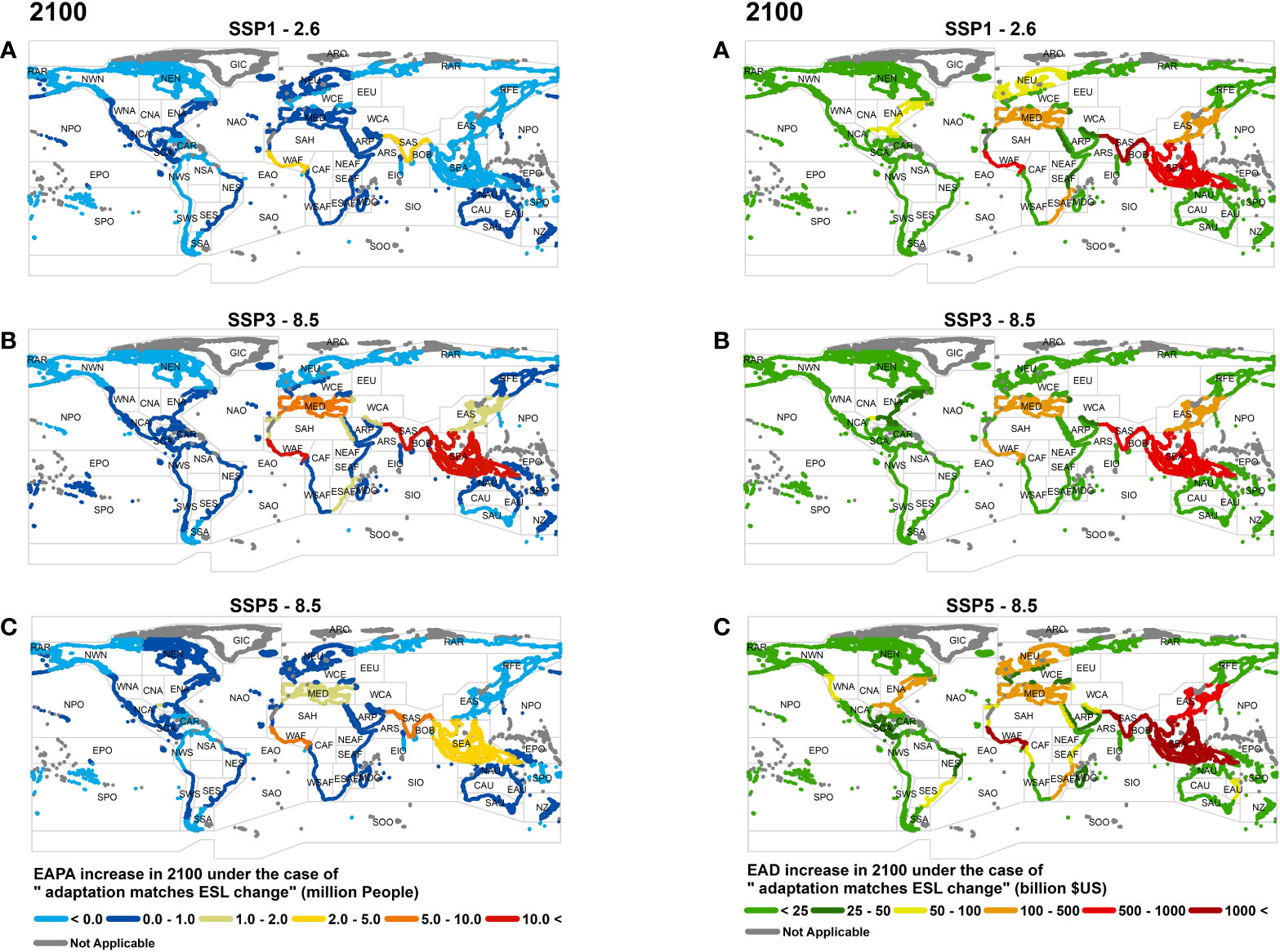
Figure 3 Changes in EAPA (left panels) and EAD (right panels) in 2100 for the scenario of adaptation matching ESL change, where adaptation measures increase over time at a rate which matches increases in ESL. Values shown represent the change relative to 2015. Panels show different Shared Socio-economic narratives (A) SSP1-2.6, (B) SSP3-8.5, (C) SSP5-8.5.
No additional adaptation scenario
The no additional adaptation scenario assumes that the flooding extent increases in the future with no changes in coastal defences and that population and GDP change with time. Figure S4 and Figure 4 show the values of EAPA and EAD for 2050 and 2100, respectively. The ranked list of regional impacts is also shown in Table 3 (top 5) and Table S7 (full list). The distribution and magnitudes of EAPA under the three different RCP/SSP combinations shown in Figure 4 (Table 3) differ markedly. In both 2050 and 2100, S. Asia and E. Asia collectively dominate in terms of EAPA under all RCP/SSP combinations. S.E Asia and Mediterranean regions are also significantly impacted for both time periods and all narratives. For the EAD, however, E. Asia ranks highest, with the exception of SSP1-2.6, where S. Asia shows the largest increase, although this is not significantly different from E. Asia.
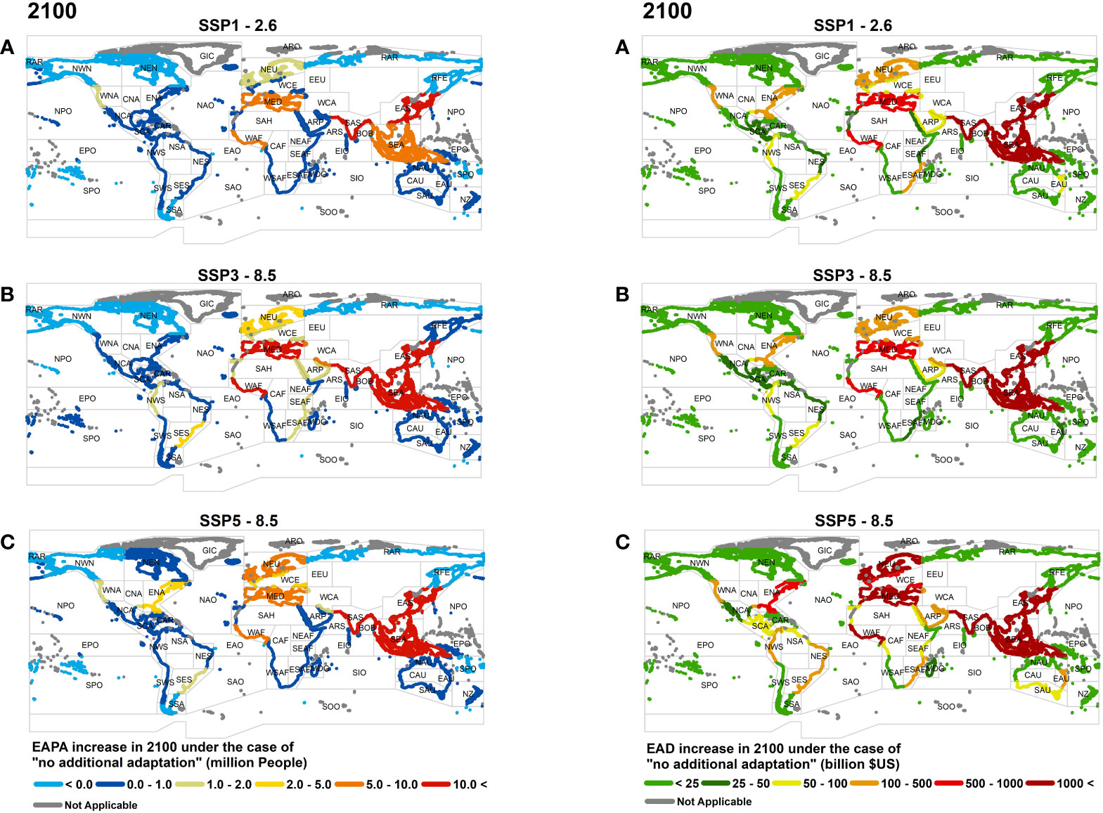
Figure 4 Changes in EAPA (left panels) and EAD (right panels) in 2100 for the scenario of no additional adaptation, where there are no changes in adaptation measures from present-day and flooding probability increases with time. Values shown represent the change relative to 2015. Panels show different RCP/SSP narratives (A) SSP1-2.6, (B) SSP3-8.5, (C) SSP5-8.5.
By 2100 (relative to 2015), the projected number of people impacted annually in E. Asia will change by between +15M and +47M (Tables 3, S7B) depending on the RCP/SSP combination. As clearly seen in Figure 4, S.E. Asia, W. Africa and the Mediterranean (largely Egypt) also show a significant change in people impacted annually by 2100 relative to 2015 (cumulatively, between +17.8M and +75.1M – Table 3). Table 3 also shows that the different SSP narratives have a striking impact on the EAPA. The values of change in EAPA for SSP3-8.5 are typically 2 to 3 times larger than those for SSP5-8.5, driven by the higher population growth under the SSP3-8.5 narrative. Although the Asian, Mediterranean and W. African regions dominate in terms of the projected increases in EAPA, the projected growth in population in N. Europe means it ranks 6th for SSP1-2.6 and SSP5-8.5 and 8th for SSP3-8.5 by 2100.
The regional distributions of EAD (Figures S4, 4 and Tables 3, S7C, D) are similar to EAPA (both for 2050 and 2100). By 2100, E. Asia shows the largest change in EAD (ranging between +US$2,376B and +US$7,063B), for SSP3-8.5 and SSP5-8.5 combinations, respectively, while S. Asia has the highest ranking for SSP1-2.6 (+US$2,594B) followed by E. Asia (+US$2,273B). For all combinations of RCP/SSP the top five regions impacted are S. Asia, E. Asia, S.E. Asia, W. Africa, and the Mediterranean by 2100. Across these 5 regions the aggregate changes in EAD are +US$6,531B (SSP3-8.5), +US$8,254B (SSP1-2.6), +US$21,969B (SSP5-8.5). Under all the SSP/RCP narratives, the developed world is also impacted by 2100 with N. Europe ranking 6th (Table S7D, +US$266B to +US$1,777B) for all narratives and E. N. America, W. N. America and W. & C. Europe in 7th and 8th position across the various narratives.
National analysis
The regional analysis described above can also be performed at the national level. Tables S8–S11 show the top 10 countries for present-day (2015) coastal flooding impacts as well as increases by 2050 and 2100 (relative to 2015) under all three cases/adaptation scenarios and RCP/SSP narratives considered. For the adaptation matching ESL change scenario, the rank order for EAPA in 2050 (Table S10A) shows India, Bangladesh, and Nigeria as the top three ranked nation for all SSP narratives. The increases in EAPA for India range between +5.3M and +8.6M, compared to the present-day country total EAPA of 7.5M. By 2100, the rank order for increase in EAPA (Table S10B) becomes more complex. Under all SSP/RCP combinations, Nigeria and India fill the first two places with collective increases in EAPA from +7.8M (SSP1-2.6) to +33.0M (SSP3-8.5), respectively. For the SSP1 and SSP5 narratives, there is much stronger population growth in the developed world compared to the developing world by 2100. As a result, the United States enters as the 4th ranked nation for SSP1-2.6 and 3rd for SSP5-8.5 (Table S10B). The absolute values of the increases in EAPA under these narratives are, however, much smaller than SSP3, which has the highest global and coastal population increase (Table 1).
The projected changes in EAD for the adaptation matching ESL change scenario show a more straightforward situation than the EAPA. For all future SSP narratives considered, India is projected to have the largest change in EAD in both 2050 and 2100 (Tables S10C, D). By 2100, the change in EAD for India ranges between +$535B (SSP3-8.5) and +$2,527B (SSP5-8.5) (Table S10D).
For the scenario of no additional adaptation, China ranks first for EAPA under SSP1-2.6 and SSP5-8.5 narratives followed by India in both 2050 and 2100 (Tables S11A, B). This rank order reverses for SSP3-8.5 for both time periods. Under this adaptation scenario, India shows an approximately two-fold increase in EAPA compared to the adaptation matching ESL change scenario, in 2100. This is typical for other nations appearing at the top 10 of EAPA for both adaptation scenarios (compare Tables S10A, S9A). For EAD, China ranks first in 2050 under all RCP/SSP combinations, with India second (Table S11C). This ranking order is retained in 2100 for SSP3-8.5 and SSP5-8.5 but reversed for SSP1-2.6.
Comparing the two adaptation scenarios in 2100 shows that these most impacted nations experience increases in EAD 2 to 3 times higher under the no additional adaptation scenario for SSP3-8.5 and SSP5-8.5. Under SSP1-2.6, however, this ratio is reduced to less than 2 (compare Tables S10D, S11D).
Tables S12A, B show the EAD as a percentage of national GDP (note: total values, not changes) for 2050 and 2100 under the no additional adaptation scenario. Whereas the absolute changes presented above illustrate the comparative impact, the percentage figures better illustrate the impact on individual nations. When expressed in this form, the differences between the various RCP/SSP combinations are much reduced at national level. By 2100, the low growth in global GDP and relatively high land area flooded yields the highest values of EAD/GDP ratio for SSP3-8.5 Table S12B). The striking feature is that developing nations are clearly the most impacted. Vietnam and Suriname dominate in terms of EAD/GDP ratio for all RCP/SSP combinations, being as high as 32.3% for Vietnam and 25.9% for Suriname. For both SSP3-8.5 and SSP5-8.5 developed nations such as Denmark and Netherlands appear in the top 20 nations with EAD/GDP ratios as high as 6%. This occurs despite the high levels of coastal protection for these nations. As the analysis considers all probability levels for the ESL, these existing coastal defences are still breached for extreme events, exacerbated by sea level rise, (resulting in greater than 1 in 10,000-year return period ESLs) with major damage resulting.
Limitations and comparison with previous studies
Limitations
A global-scale analysis of the type undertaken here requires a number of simplifying assumptions to make the problem tractable. This analysis extends the approach of Kirezci et al. (2020) to probability levels other than 1 in 100 years and integrates these values to determine EAPA and EAD. Kirezci et al. (2020) validated their extreme value analysis approach against an extensive network of global historical tide gauge data (see Kirezci et al., 2020, their Figures S2, S3, S7 and Tables S1, S2). This same extreme value analysis was adopted here (i.e. Generalized Pareto Distribution). The future projections of ESL do not, however, include possible changes in extreme values of surge, tide levels and wave climate over the coming century, which were assumed small compared to the effect relative sea level rise has on changes in ESLs. Extreme value analyses as undertaken here are stochastic projections and hence involve uncertainty. Following Kirezci et al. (2020), the 90th percentile confidence limits on all projections were calculated using a bootstrap approach (see Materials and Methods) and are shown in Tables 2, S1-S3.
Coastal adaptation strategies can be broadly defined as coastal protection, accommodation, and retreat (Diaz, 2016). The present analysis considers the adaptation strategy in the form of coastal protection by structural measures (e.g. dikes), similar to previous analyses (Nicholls, 2002; Hinkel et al., 2014; Lincke and Hinkel, 2018; Nicholls et al., 2019; Tamura et al., 2019; Tiggeloven et al., 2020; Vousdoukas et al., 2020; Brown et al., 2021). Coastal protection by structural measures is commonly applied in impact studies because it delivers more predictable safety levels against coastal extremes (Vousdoukas et al., 2020) to estimate the future costs of adaptation. However, other adaptation alternatives may be considered to determine future cost, such as accommodation, which allows permanent inundation up to a certain damage limit. This may be achieved by, for example, raising structures, and retreat from the coastline (Diaz, 2016). For example, Lincke and Hinkel (2021) showed that along with the coastal protection, coastal retreat is economically robust for most coastal areas. Over time, as the socioeconomic drivers change, the most appropriate adaptation strategy and rate of application may change. This may particularly take place when lower probability ESLs become more frequent due to the impact of the SLR. However, the main purpose in this study is to demonstrate the lower and the upper limits of the impacts of “no additional adaptation” compared to outcomes of raising the sea dikes at the same pace as ESL change. While we acknowledge that this approach is limited to one type of adaptation (i.e., coastal protection by structural measures), the results illustrate the significant differences of impacts for “protection” and “no further action” at global, regional and national scales, in terms of EAPA and EAD.
A “bathtub” flooding approach has been assumed to estimate areas impacted by coastal flooding. Such an approach ignores the attenuation of the overland flooding and potentially overestimates the potential impacts (Vafeidis et al., 2019). However, at global scale a more detailed flooding approach is not practical.
The population data (GPWv4) uses an areal dataset with 30arcsec resolution. This dataset relies on a uniform allocation model to disaggregate census estimations. This will introduce local uncertainty in values. However, the resolution of this dataset is consistent with other data used in the global-scale analysis.
No global dataset of absolute values of coastal protection is available. Rather, the DIVA database (Hinkel and Klein, 2009) contains values of the design return periods on a sub-national basis. These were used here with an assumed probability distribution (see Materials and Methods) to estimate the corresponding protection levels. Although such an approach is consistent with design standards in each nation, whether such protection levels are always followed is unknown. This will result in uncertainties in some areas regarding the exact levels of present-day coastal protection.
A commonly used depth-damage relation, Eq. (1) (Main manuscript), (Hinkel et al., 2014) is used to estimate infrastructure damage given the depth of flooding and value of assets exposed. Although this approach has precedence in the literature, it is a global average value and will vary in specific locations giving rise to uncertainty.
The EAPA and EAD were estimated from integration of the probability distribution function of extreme flooding extent (as outlined in the Methods Section within the main manuscript). Based on the results of Kirezci et al. (2020) a Generalized Pareto Distribution (GPD) was assumed (see Materials and Methods) for all the return period values of ESLs. If an alternative distribution had been used, there will be variation in these resulting values. However, the GPD has been shown to fit both modelled and measured ESL optimally (Kirezci et al., 2020).
The present analysis does not include land subsidence due to human induced groundwater or gas extraction, which may result in underestimation of the flooding impacts. Although regional relative sea level rise has the greatest impact on the increased coastal flooding extent, groundwater extraction poses a great challenge especially for densely populated coastal delta regions (Ericson et al., 2006; Syvitski et al., 2009; Tiggeloven et al., 2020). However, it is difficult to estimate and model projections of groundwater extraction at the global scale, as these trends are subject to change in time and are highly dependent on the dynamics of local communities (Hinkel et al., 2014).
Similarly, the analysis does not consider the impact of compound events such as joint storm surge and river flooding (Khanal et al., 2019). In areas such as estuaries of substantial rivers, this omission can underestimate flooding extent.
Comparison with previous studies
Direct comparisons between the present study and previous global analyses (Tiggeloven et al., 2020; Hinkel et al., 2014; Diaz, 2016; Tamura et al., 2019; Schinko et al., 2020) are difficult due to differences in the methodologies and datasets used, which can result in large variations between the detailed findings. Nevertheless, there is general consensus across most of these studies, particularly in terms of the importance of future adaptation. Different studies assume a variety of different adaptation approaches and levels, making quantitative comparisons impossible. A common approach, however, is to determine the impacts “without future adaptation” (Hinkel et al., 2014) (as in the no additional adaptation scenario in this study). Therefore, here we confine comparisons to previous coastal flooding studies that consider present-day defence levels but do not account for any future adaptation by 2100.
• Hinkel et al. (2014), applied a range of datasets and adaptation strategies to account for uncertainties in coastal flood impact projections and adaptation cost estimates. Factors considered include: a range of regional sea level rise scenarios, population and asset exposure as well as socioeconomic scenarios SSP1-5. They found 2100 values of global EAPA of: 0.2% - 2.9% (RCP 2.6) and 0.5% - 4.6% (RCP8.5) of global population. Values of EAPA for the present study as a percentage of global population can be obtained from Table S3 and Table 2. Including the span of the 90th percentile confidence limits, this yields values between 0.9% and 2.6% across all combinations of RCP/SSP. Hinkel et al. (2014) also found 2100 values of EAD ranging between 0.3 - 5.0% GDP (RCP 2.6) and 1.2% – 9.3% (RCP8.5), compared to 1.2% to 4.1% obtained in this study across all combinations of RCP/SSP (Table 2). The higher range given by Hinkel et al. (2014) can be partially explained by their ranges being based on the two digital elevation data sets GLOBE and SRTM (of which MERIT used here is derived). GLOBE delivers an exposure approximately twice as high as SRTM. Hence, we conclude that the present results are of comparable magnitude to the Hinkel et al. (2014) projections with the differences consistent with the respective datasets used.
• Tiggeloven et al. (2020) determined global adaptation costs by 2080 for SSP5-8.5, obtaining a range of US$3T to $US6.8T/year. Table S3 shows values of EAD for SSP5-8.5 of US$2.6T to US$7.8T in 2050 and US$20.0T to US$39.8T by 2100 for the present study. Therefore, the Tiggeloven et al. (2020) 2080 values overlap these limits, indicating the studies yield results of comparable magnitude.
• Schinko et al. (2020) considered economic impacts addressing the macro-economic implications of coastal flooding together with the direct damage and found that in the absence of the future adaptation, under SSP2-2.6 and SSP2-4.5, by 2050 the global EAD would be 0.17% - 0.55% (SSP2-4.5) and 0.13% - 0.54% (SSP2-2.6) of GDP. This compares to values between 0.62% and 2.16% (Table 2) across all combinations of RCP/SSP by 2050 in the present study. By 2100 Schinko et al. (2020) project a global EAD of 1.5% - 4.5% (SSP2-4.5) and 0.6% - 3.5% of GDP (SSP2-2.6). In comparison, the present study projects a global EAD of between 1.2% and 4.1% of GDP by 2100 across all combinations of RCP/SSP. Noting the different methodologies and SSP narratives used, the results are comparable.
As noted above, these previous studies produce a very large range of EAPA and EAD values, and due to differences in methodology and datasets used, direct comparisons with the present study are difficult. Noting this, the present results span these previous results, but are at the upper end of this range. We believe this occurs because of the flood protection levels and methodology used (see Materials and Methods) and the use of the SROCC relative sea level rise values.
Although the above comparisons provide a degree of confidence in application of the results of the present study to future projections at the regional/global scale, the many assumptions and limitations means that such studies need to be applied with caution (Hinkel et al., 2021). Further comparison studies, particularly comparing finer-scale regional models and global assessments are recommended.
Discussion and conclusions
Many global-scale analyses of future coastal flooding consider the impacts of episodic events such as 1 in 100-year floods and, where they extend this to socio-economic consideration, the populations potentially impacted and the assets exposed to damage (Nicholls and Tol, 2006; Nicholls et al., 2007; Jongman et al., 2012; Neumann et al., 2015; Muis et al., 2016; Muis et al., 2017; Brown et al., 2018; Kulp and Strauss, 2019; Vafeidis et al., 2019; Kirezci et al., 2020). Such studies provide a valuable understanding of potential “hot-spots” where episodic coastal flooding is likely to be a significant problem. However, aggregation of the results tends to significantly overestimate potential impacts. To address these issues, further studies have estimated actual damage to assets, rather than the total value of assets exposed, have estimated the impacts of coastal defences and determined annual values of EAPA and EAD rather than values at a single extreme value probability level (e.g. 1 in 100 years) (Hallegatte et al., 2013; Vousdoukas et al., 2018b; Hinkel et al., 2014; Diaz, 2016; Brown et al., 2016; Lincke and Hinkel, 2018; Tamura et al., 2019; Schinko et al., 2020; Tiggeloven et al., 2020). The present analysis follows this general methodology and builds on the recent analysis of (Kirezci et al., 2020). The analysis considers: expected annual values rather than 1 in 100-year values over the 21st century using recent IPCC SROCC RCP 2.6, RCP 4.5 and RCP 8.5 sea level rise scenarios (Oppenheimer et al., 2019), estimates of the present levels of coastal protection in place and plausible scenarios for future changes in defence levels, value of infrastructure damage rather than assets exposed and considers how population and GDP may change in the future.
Impacts for the world
Our results demonstrate that both projected changes in episodic coastal flooding and changes in future population and GDP result in substantial differences between the present and future coastal flood impacts in terms of people affected and damage caused to infrastructure. Without any future adaptation (no additional adaptation scenario), global EAPA and EAD in 2100 change by +212M people/year (Table S3, SSP3-8.5) and +US$27,736B/year (Table S3, SSP5-8.5), relative to 2015. As noted above, these estimates are sensitive to assumptions made in computing flooding extent, coastal topography databases used and projected changes in population and GDP. Previous studies produce a wide range of values (see SM Comparison with Previous Studies section), with the results of the present study falling within the values of these previous studies (Hinkel et al., 2014; Schinko et al., 2020; Tiggeloven et al., 2020). Our results indicate that under even a simplistic adaptation approach (adaptation matching ESL change scenario) where the height of coastal defences are adjusted at the same rate as ESL change, the total values of additional people affected by coastal flooding, EAPA, are significantly reduced (Tables S2, S3; SSP3-8.5), by a factor of 2.5 (212M/85M) in 2100. Similarly, the total EAD increase is reduced (Tables S2, S3; SSP5-8.5), by a factor of 2.7 ($27,736B/$10,120B).
The regional impacts of adaptation can be assessed by comparison of the adaptation matching ESL change and no additional adaptation scenarios in 2100 for EAPA (Tables S6B, S7B) and EAD (Tables S6D, S7D). The inclusion of the adaptation measures in the adaptation matching ESL change scenario (for the SSP3-8.5 narrative) results in a decrease in total values of increases in EAPA for E. Asia by a factor of 38.9; Mediterranean by 2.4; S. Asia by a factor of 2.1; S.E. Asia by 1.9; and W. Africa by 1.2. The impact of adaptation on total increases in EAD by 2100 shows similar regional variability (for the SSP5-8.5 narrative) with E. Asia decreasing by a factor of 13.6; Mediterranean by 4.7; S. Asia by 1.9; S.E. Asia by 1.9; and W. Africa by 1.2. Therefore, although the additional adaptation shows significant benefits in all areas, the returns vary appreciably both for EAPA and EAD by region with E.Asia seeing the largest returns for this additional adaptation.
A comparison of global present-day values of EAPA with the no additional adaptation scenario values in 2100 (no changes to adaptation and SSP3-8.5) projects an increase by a factor of 7.2 (212 + 34/34) in the total number of people impacted (Table S3). For EAD the increase relative to present-day values is a factor as large as 90 (SSP5-8.5, 27,376 + 307/307), (Table S3). The regional changes between present-day and the no additional adaptation scenario in 2100 show significant regional variation from these global values. For EAPA, we project increases for (compare Table S4A with SSP3-8.5, Table S7B): Mediterranean by a factor of 19.9; E. Asia by 14.6; W. Africa by 6.7; S. Asia by 6.5; and S.E. Asia by 4.3. The corresponding increases in values for EAD by 2100 are (compare Table S4B with SSP5-8.5, Table S7D): Mediterranean by a factor of 167; W. Africa by 123; E. Asia by 111; S. Asia by 106; and S.E. Asia by 49.
These results show that adaptation measures will be a critical element of addressing episodic coastal flooding under any plausible RCP/SSP narrative, as they significantly reduce projected EAPA and EAD. However, the impacts of coastal flooding will disproportionally fall on the developing world, both in absolute terms and relative to GDP. As shown in Table 3, by 2100 the largest increases in both EAPA and EAD will be borne by S. Asia, S.E. Asia, E. Asia, W. Africa and the Mediterranean (Egypt). The only developed region that ranks in the top 5 for any of the narratives is N. Europe, but on a much smaller scale than these developing regions. The relative impact on EAD in the developing world is clearly seen in Table S12B which shows the EAD as a percentage of GDP by country in 2100 for the no additional adaptation scenario. The top ten nations in the world ranking are dominated by developing countries such as: Vietnam, Suriname, Guyana, Myanmar, and Bangladesh. All of these nations have an EAD in excess of almost 7% of their GDP, even for the “sustainable world – Paris agreement” narrative of the RCP/SSP combination (i.e. SSP1-2.6).
For the developed world, Japan, exceeds 4% of the nation’s EAD/GDP ratio by 2100 under all RCP/SSP combinations, whereas low-lying N. European nations, such as Netherlands and Denmark; as well as the UK, have an EAD/GDP ratio as high as 6% under SSP3-8.5 and SSP5-8.5 pathways. However, these impacts could reasonably be addressed with additional adaptation measures. Most of the developed world have an EAD of less than 3.5% of GDP, with the global mean EAD being 2.9% (Table 2, no additional adaptation scenario). At these levels, it is likely that developed nations will be able to cope with impacts of this magnitude without major disruption. However, the developing world will face major disruption.
Figure 5 shows an infographic of the EAD as a percentage of national GDP for selected nations. The results are shown for both SSP1-2.6 (Figure 5A) and SSP3-8.5 (Figure 5B) and the two adaptation scenarios: no additional adaptation and adaptation matching ESL change. This figure clearly illustrates that the major impacts of flooding will fall on the developing world and that globally, these impacts can be significantly reduced by further mitigation of atmospheric emission levels (SSP/RCP narrative) as well as future adaptation measures.
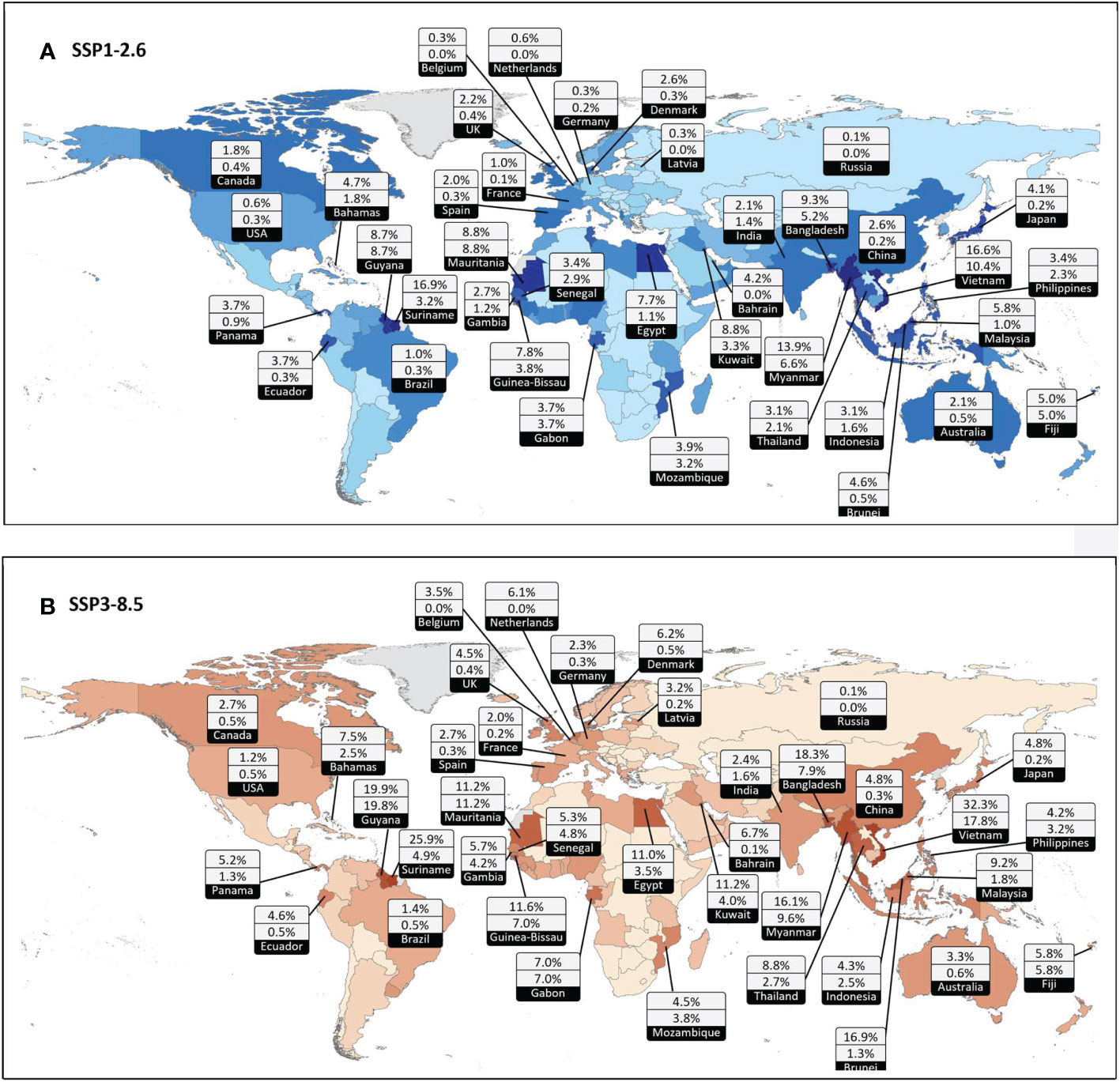
Figure 5 Infographic showing national percentage EAD of GDP for (A) SSP1-2.6 and (B) SSP3-8.5. For each “data bubble” the top figure is the no additional adaptation scenario and the bottom number is adaptation matching ESL change scenario. Nation colour code (from lighter to darker) is proportional to percentage EAD for no additional adaptation scenario (top number). Map national boundaries from NASA Socioeconomic Data and Applications Center (SEDAC) (https://sedac.ciesin.columbia.edu/data/collection/gpw-v4).
Application and significance
As noted throughout the paper, the physical processes active in coastal inundation need to be significantly simplified for such a global-scale analysis. These necessary assumptions to undertake such a global analysis may mean that results at a particular location may be inaccurate. However, when aggregated to national and regional scale, the analysis provides a first-pass assessment of the projected socio-economic impacts of episodic coastal flooding.
As such, the results form the basis for consideration of the potential impacts on different nations of future coastal flooding. The analysis forms a useful tool to further assess the relative impacts on different nations of climate change. Applications of the data could include: providing guidance for policy makers on potential adaptation strategies, understanding potential future economic costs of coastal flooding and informing discussions of climate financing which may be paid by developed countries to developing nations.
Data availability statement
The original contributions presented in the study are included in the article/Supplementary Material. Further inquiries can be directed to the corresponding author.
Author contributions
EK conducted most of the analysis. IY conceived the project. EK, IY, RR, DL and JH contributed to the development of the project and the written paper. All authors contributed to the article and approved the submitted version.
Funding
IY gratefully acknowledges the support of the Australian Research Council through grants DP130100215, DP160100738 and DP210100840. RR is supported by the AXA Research Fund and the Deltares Strategic Research Programme “Risk Management”.
Acknowledgments
The GOW2 data used to determine breaking wave setup were generously supplied by Melisa Menendez. The storm surge data used to determine the global extreme flooding levels was provided by Sanne Muis.
Conflict of interest
The authors declare that the research was conducted in the absence of any commercial or financial relationships that could be construed as a potential conflict of interest.
Publisher’s note
All claims expressed in this article are solely those of the authors and do not necessarily represent those of their affiliated organizations, or those of the publisher, the editors and the reviewers. Any product that may be evaluated in this article, or claim that may be made by its manufacturer, is not guaranteed or endorsed by the publisher.
Supplementary material
The Supplementary Material for this article can be found online at: https://www.frontiersin.org/articles/10.3389/fmars.2022.1024111/full#supplementary-material
References
Abadie L., Sainz de Murieta E., Galarraga I. (2016). Climate risk assessment under uncertainty: An application to main European coastal cities. Front. Mar. Sci. Volume 3. doi: 10.3389/fmars.2016.00265
Antunes C., Rocha C., Catita C. (2019). Coastal flood assessment due to sea level rise and extreme storm events: A case study of the atlantic coast of portugal’s mainland. Geosciences 9, 239. doi: 10.3390/geosciences9050239
Brown S., Nicholls R. J., Goodwin P., Haigh I. D., Lincke D., Vafeidis A. T., et al. (2018). Quantifying land and people exposed to sea-level rise with no mitigation and 1.5 c and 2.0 c rise in global temperatures to year 2300. Earth's Future 6, 583–600. doi: 10.1002/2017EF000738
Brown S., Jenkins K., Goodwin P., Lincke D., Vafeidis A. T., Tol R. S., et al. (2021). Global costs of protecting against sea-level rise at 1.5 to 4.0 °C. Climatic Change 167 (1), 1–21. doi: 10.1007/s10584-021-03130-z
Brown S., Nicholls R. J., Lowe J. A., Hinkel J. (2016). Spatial variations of sea-level rise and impacts: An application of DIVA. Climatic Change 134, 403–416. doi: 10.1007/s10584-013-0925-y
Carrere L., Lyard F., Cancet M., Guillot A. (2015). FES2014, a new tidal model on the global ocean with enhanced accuracy in shallow seas and in the Arctic region (Vienna, Austria).
Center for International Earth Science Information Network (CIESIN) (2018). Documentation for the gridded population of the world, version 4 (Palisades NY: Columbia Univ.).
Church J. A., Clark P. U., Cazenave A., Gregory J. M., Jevrejeva S., Levermann A., et al. (2013). “Sea Level change,” in Climate change 2013: The physical science basis. contribution of working group I to the fifth assessment report of the intergovernmental panel on climate change (New York: Cambridge University Press), 1137–1216.
Dee D., Uppala S. M., Simmons A. J., Berrisford P., Poli P., Kobayashi S., et al. (2011). The ERA-interim reanalysis: configuration and performance of the data assimilation system. Q. Jnl. R. Met. Soc 137, 553–597. doi: 10.1002/qj.828
Diaz D. (2016). Estimating global damages from sea level rise with the coastal impact and adaptation model (CIAM). Climate Change 137, 143–156. doi: 10.1007/s10584-016-1675-4
Efron B. (1979). Bootstrap methods: Another look at the jacknife. Ann. Stats. 7, 1–26. doi: 10.1214/aos/1176344552
Ericson J. P., Vörösmarty C. J., Dingman S. L., Ward L. G., Meybeck M. (2006). Effective sea-level rise and deltas: Causes of change and human dimension implications. Global Planetary Change 50 (1–2), 63–82.
Fang J., Lincke D., Brown S., Nicholls R. J., Wolff C., Merkens J. L., et al. (2020). Coastal flood risks in China through the 21st century – an application of DIVA. Sci. Total Environ. 704 (135311), 1–12. doi: 10.1016/j.scitotenv.2019.135311
Farr T., Rosen P. A., Caro E., Crippen R., Duren R., Hensley S., et al. (2007). The shuttle radar topography mission. Rev. Geophysics 45 (2), 1–33. doi: 10.1029/2005RG000183
Fyfe J. C., Kharin V. V., Santer B. D., Cole J. N., Gillett N. P. (2021). Significant impact of forcing uncertainty in a large ensemble of climate model simulations. Proc. Natl. Acad. Sci. United States America 118 (6), 1–6. doi: 10.1073/pnas.2016549118
Gao J. (2017). Downscaling global spatial population projections from 1/8-degree to 1-km grid cells. (Boulder, CO, USA: National Center for Atmospheric Research), 1105. doi: 10.5065/D60Z721H
Haigh I. D., Pickering M. D., Green J. M., Arbic B. K., Arns A., Dangendorf S., et al. (2019). The tides they are a-changin': A comprehensive review of past and future nonastronomical changes in tides, their driving mechanisms and future implications. Rev. Geophysics 57, e2018RG000636. doi: 10.1029/2018RG000636
Haigh I., Nicholls R., Penning-Rowsell E., Sayers P. (2020). Impacts of climate change on coastal flooding, relevant to the coastal and marine environment around the UK. MCCIP Sci. Rev. 2020, 546–565. doi: 10.14465/2020.arc23.cfl
Hallegatte S., Green C., Nicholls R., Corfee-Morlot J. (2013). Future flood loses in major coastal cities. Nat. Clim. Change 3, 802–806. doi: 10.1038/nclimate1979
Hauer M., Evans J., Mishra D. (2016). Millions projected to be at risk from sea-level rise in the continental united states. Nat. Climate Change 6, 691–695. doi: 10.1038/nclimate2961
Hinkel J., Lincke D., Vafeidis A. T., Perrette M., Nicholls R. J., Tol R. S., et al. (2014). Coastal flood damage and adaptation costs under 21st century sea-level rise. Proc. Nat. Acad. Sci. 111, 3292–3297. doi: 10.1073/pnas.1222469111
Hinkel J., Feyen L., Hemer M., Le Cozannet G., Lincke D., Marcos M., et al. (2021). Uncertainty and bias in global to regional scale assessments of current and future coastal flood risk. Earth's Future 9 (7), e2020EF001882. doi: 10.1029/2020EF001882
Hinkel J., Klein R. (2009). Integrating knowledge to assess coastal vulnerability to sea-level rise: The development of the DIVA tool. Global Environ. Change 19 (3), 384–395. doi: 10.1016/j.gloenvcha.2009.03.002
Hunter J., Woodworth P., Wahl T., Nicholls R. (2017). Using global tide gauge data to validate and improve the representation of extreme sea levels in flood impact studies. Global Planetary Change 156, 34–45. doi: 10.1016/j.gloplacha.2017.06.007
Idier D., Bertin X., Thompson P., Pickering M. (2019). Interactions between mean Sea level, tide, surge, waves and flooding: Mechanisms and contributions to Sea level variations at the coast. Surv. Geophys. 40, 1603–1630. doi: 10.1007/s10712-019-09549-5
Iturbide M., Gutiérrez J. M., Alves L. M., Bedia J., Cerezo-Mota R., et al. (2020). An update of IPCC climate reference regions for subcontinental analysis of climate model data: Definition and aggregated datasets. Earth Sys. Sci. Data 12 (4), 2959–2970. doi: 10.5194/essd-12-2959-2020
Jarvis A., Reuter H., Nelson A., Guevara E. (2008) Hole-filling SRTM for the globe, version 4. Available at: http://srtm.csi.cgiar.org.
Jones B., O’Neill B. (2016). Spatially explicit global population scenarios consistent with the shared socioeconomic pathways. Environ. Res. Lett. 11, 84003. doi: 10.1088/1748-9326/11/8/084003
Jongman B., Ward P., Aerts J. (2012). Global exposure to river and coastal flooding: Long term trends and changes. Global Environ. Change 22 (4), 823–835. doi: 10.1016/j.gloenvcha.2012.07.004
Khanal S., Ridder N., De Vries H., Terink W., Van den Hurk B., et al. (2019). Storm surge and extreme river discharge: A compound event analysis using ensemble impact modeling. Front. Earth Sci. 7 (224). doi: 10.3389/feart.2019.00224
Kirezci E., Young I. R., Ranasinghe R., Muis S., Nicholls R. J., Lincke D., et al. (2020). Projections of global-scale extreme sea levels and resulting episodic coastal flooding over the 21st century. Sci. Rep. 10 (1), 1–12. doi: 10.1038/s41598-020-67736-6
Kulp S., Strauss B. (2019). New elevation data triple estimates of global vulnerability to sea-level rise and coastal flooding. Nat. Commun. 10 (1), 1–12. doi: 10.1038/s41467-019-12808-z
Kummu M., Taka M., Guillaume J. (2018). Gridded global datasets for gross domestic product and human development index over 1990–2015. Sci. Data. 5, 180004. doi: 10.1038/sdata.2018.4
Lincke D., Hinkel J. (2018). Economically robust protection against 21st century sea-level rise. Global Environ. Change 51, 67–73. doi: 10.1016/j.gloenvcha.2018.05.003
Lincke D., Hinkel J. (2021). Coastal migration due to 21st century Sea-level rise. Earth's Future 9 (5), e2020EF001965. doi: 10.1029/2020EF001965
Lyard F. H., Allain D. J., Cancet M., Carrère L., Picot N. (2021). FES2014 global ocean tide atlas: design and performance. Ocean Sci 17 (3), 615–649.
MacManus K., Balk D., Engin H., McGranahan G., Inman R. (2021). Estimating population and urban areas at risk of coastal hazards 1990–2015: how data choices matter. Earth System Sci. Data 13, 5747–5801. doi: 10.5194/essd-13-5747-2021
McGranahan G., Balk D., Anderson B. (2007). The rising tide: assessing the risks of climate change and human settlements in low elevation coastal zones. Environ. Urbanization 19, 17–37. doi: 10.1177/0956247807076960
Marcos M., Rohmer J., Vousdoukas M. I., Mentaschi L., Le Cozannet G., Amores A. (2019). Increased extreme coastal water levels due to the combined action of storm surges and wind waves. Geophys. Res. Lett. 46 (8), 4356–4364. doi: 10.1029/2019GL082599
Melet A., Meyssignac B., Almar R., Le Cozannet G. (2018). Under-estimated wave contribution to coastal sea-level rise. Nat. Climate Change 8, 234–239. doi: 10.1038/s41558-018-0088-y
Messner F. (2007). Evaluating flood damages: guidance and recommendations on principles and methods. T09-06-01. Available at: http://resolver.tudelft.nl/uuid:5602db10-274c-40da-953f-34475ded1755.
Meucci A., Young I., Breivik O. (2018). Wind and wave extremes from atmosphere and wave model ensembles. J. Clim. 31, 8819–8893. doi: 10.1175/JCLI-D-18-0217.1
Meyer V., Scheuer S., Haase D. (2009). A multicriteria approach for flood risk mapping exemplified at the mulde river, Germany. Natural Hazards 48 (1), 17–39. doi: 10.1007/s11069-008-9244-4
Milne G., Gehrels W., Hughes C., Tamisiea M. (2009). Identifying the causes of sea-level change. Nat. Geosci. 2, 471–478. doi: 10.1038/ngeo544
Muis S., Güneralp B., Jongman B., Aerts J. C., Ward P. J.. (2015). Flood risk and adaptation strategies under climate change and urban expansion: A probabilistic analysis using global data. Sci. Total Environ. 538, 445–457. doi: 10.1016/j.scitotenv.2015.08.068
Muis S., Verlaan M., Winsemius H. C., Aerts J. C., Ward P. J. (2016). A global reanalysis of storm surges and extreme sea levels. Nat. Commun. 7, 11969. doi: 10.1038/ncomms11969
Muis S., Verlaan M., Nicholls R. J., Brown S., Hinkel J., Lincke D., et al. (2017). A comparison of two global datasets of extreme sea levels and resulting flood exposure. Earth’s Future 5 (4), 379–392. doi: 10.1002/2016EF000430
Neumann B., Vafeidis A. T., Zimmermann J., Nicholls R. J. (2015). Future coastal population growth and exposure to Sea-level rise and coastal flooding - a global assessment. PLoS One 10, e0118571. doi: 10.1371/journal.pone.0118571
Nicholls R. J. (2002). Analysis of global impacts of sea-level rise: a case study of flooding. Phys. Chem. Earth Parts A/B/C 27 (32-34), 1455–1466. doi: 10.1016/S1474-7065(02)00090-6
Nicholls R., Cazenave A. (2010). Sea-Level rise and its impact on coastal zones. Science 328, 1517–1520. doi: 10.1126/science.1185782
Nicholls R. J., Hanson S., Herweijer C., Patmore N., Hallegatte S., Corfee-Morlot J., et al. (2007). Ranking of the world’s cities most exposed to coastal flooding today and in the future. organisation for economic Co-operation and development. OECD (Paris).
Nicholls R., Brown S., Goodwin P., Wahl T., Lowe J., Solan M., et al. (2018). Stabilization of global temperature at 1.5°C and 2.0°C: implications for coastal areas. Philos. Trans. R. Soc. A: Mathematical Phys. Eng. Sci. 376, 20160448. doi: 10.1098/rsta.2016.0448
Nicholls R. J., Hinkel J., Lincke D., van der Pol T. (2019). Global investment costs for coastal defense through the 21st century (Washington, DC: © World Bank).
Nicholls R. J., Tol R. S. (2006). Impacts and responses to sea-level rise: a global analysis of the SRES scenarios over the twenty-first century. Phil. Trans. R. Soc A 364, 1073–1095. doi: 10.1098/rsta.2006.1754
O'Neill B., Carter T. R., Ebi K., Harrison P. A., Kemp-Benedict E., Kok K., et al. (2020). Achievements and needs for the climate change scenario framework. Nat. Climate Change 10, 1074–1084. doi: 10.1038/s41558-020-00952-0
O’Neill B., Kriegler E., Riahi K., Ebi K. L., Hallegatte S., Carter T. R., et al. (2014). A new scenario framework for climate change research: the concept of shared socioeconomic pathways. Climatic Change, 122 (3), 387–400. doi: 10.1007/s10584-013-0905-2
Oppenheimer M., Glavovic B. C., Hinkel J., Wal van R., Magnan A. K., Abd-Elgawad A., et al. (2019). “Sea Level rise and implications for low-lying islands, coasts and communities,” in IPCC special report on the ocean and cryosphere in a changing climate. Eds. Pörtner H.-O., Roberts D. C., Masson-Delmotte V., Zhai P., Tignor M., Poloczanska E., Mintenbeck K., Alegría A., Nicolai M., Okem A., Petzold J., Rama B., Weyer N. M.. In press.
Perez J., Menendez M., Losada I. (2017). GOW2: A global wave hindcast for coastal applications. Coast. Eng. 124, 43405. doi: 10.1016/j.coastaleng.2017.03.005
Reguero B. G. L. I. J., Diaz-Simal P., Mendez F. J., Beck M. W. (2015). Effects of climate change on exposure to coastal flooding in Latin America and the Caribbean. PLoS One 10 (7), e0133409. doi: 10.1371/journal.pone.0133409
Riahi K., Van Vuuren D. P., Kriegler E., Edmonds J., O’neill B. C., Fujimori S., et al. (2017). The shared socioeconomic pathways and their energy, land use, and greenhouse gas emissions implications: An overview. Global Environ. Change 42, 153–168. doi: 10.1016/j.gloenvcha.2016.05.009
Rio M., Mulet S., Picot N. (2014). Beyond GOCE for the ocean circulation estimate: Synergetic use of altimetry, gravimetry, and in situ data provides insight into geostrophic and ekman currents. Geophys. Res. Lett. 41 (24), 8918–8925. doi: 10.1002/2014GL061773
Rueda A., Vitousek S., Camus P., Tomás A., Espejo A., Losada I. J., et al. (2017). A global classification of coastal flood hazard climates associated with large-scale oceanographic forcing. Scientitic Rep. 7, 5038. doi: 10.1038/s41598-017-05090-w
Sadoff C., Hall J.W., Grey D., Aerts J. C. J. H., Ait-Kadi M., Brown C., et al. (2015). Securing water, sustaining growth: Report of the GWP/OECD task force on water security and sustainable growth (UK: University of Oxford). 180pp.
Schinko T., Drouet L., Vrontisi Z., Hof A., Hinkel J., Mochizuki J., et al. (2020). Economy-wide effects of coastal flooding due to sea level rise: a multi-model simultaneous treatment of mitigation, adaptation, and residual impacts. Environ. Res. Commun. 2 (1), 015002. doi: 10.1088/2515-7620/ab6368
Stockdon H., Holman R., Howd P., Sallenger A. (2006). Empirical parameterization of setup, swash, and runup. Coast. Eng. 53, 573–588. doi: 10.1016/j.coastaleng.2005.12.005
Syvitski J. P., Kettner A. J., Overeem I., Hutton E. W., Hannon M. T., Brakenridge G. R., et al (2009). Sinking deltas due to human activities. Nat Geoscie 2 (10), 681–686.
Tamura M., Kumano N., Yotsukuri M., Yokoki H. (2019). Global assessment of the effectiveness of adaptation in coastal areas based on RCP/SSP scenarios. Climatic Change 152 (3), 363–377. doi: 10.1007/s10584-018-2356-2
Tiggeloven T., Winsemius H. C., Eilander D., Erkens G., Gebremedhin E., et al. (2020). Global-scale benefit–cost analysis of coastal flood adaptation to different flood risk drivers using structural measures. Nat. Hazards Earth Syst. Sci. 20 (4), 1025–1044. doi: 10.5194/nhess-20-1025-2020
Vafeidis A., Nicholls R. J., McFadden L., Tol R. S., Hinkel J., Spencer T., et al. (2008). A new global coastal database for impact and vulnerability analysis to sea-level rise. J. Coast. Res. 24 (4), 917–924. doi: 10.2112/06-0725.1
Vafeidis A., Schuerch M., Wolff C., Spencer T., Merkens J. L., Hinkel J., et al. (2019). Water-level attenuation in global-scale assessments of exposure to coastal flooding: a sensitivity analysis. Nat. Hazards Earth Syst. Sci. 19 (5), 973–984. doi: 10.5194/nhess-19-973-2019
van Vuuren D., Carter T. (2014). Climate and socio-economic scenarios for climate change research and assessment: reconciling the new with the old. Climatic Change 122 (3), 415–429. doi: 10.1007/s10584-013-0974-2
Vitousek S., Barnard P. L., Fletcher C. H., Frazer N., Erikson L., Storlazzi C. D. (2017). Doubling of coastal flooding frequency within decades due to sea-level rise. Sci. Rep. 1399, 1–9. doi: 10.1038/s41598-017-01362-7
Vousdoukas M. I., Mentaschi L., Voukouvalas E., Verlaan M., Jevrejeva S., Jackson L. P., et al. (2018a). Global probabilistic projections of extreme sea levels show intensification of coastal flood hazard. Nat. Commun. 9, 2360. doi: 10.1038/s41467-018-04692-w
Vousdoukas M., Mentaschi L., Voukouvalas E., Bianchi A., Dottori F., Feyen L.. (2018b). Climatic and socioeconomic controls of future coastal flood risk in Europe. Nat. Climate Change, 776–780. doi: 10.1038/s41558-018-0260-4
Vousdoukas M., Mentaschi L., Hinkel J., Ward P. J., Mongelli I., Ciscar J. C., et al. (2020). Economic motivation for raising coastal flood defences in Europe. Nat. Comms. 11, 2119. doi: 10.1038/s41467-020-15665-3
Wessel P., Smith W. (1996). A global self-consistent, hierarchical, high-resolution shoreline database. J. Geophys. Res. 101, 8741–8743. doi: 10.1029/96JB00104
Woodworth P., Hunter J. R., Marcos M., Caldwell P., Menéndez M., Haigh I. (2017). Towards a global higher-frequency sea level dataset. Geosci. Data J. 3, 50–59. doi: 10.1002/gdj3.42
Yamazaki D., Ikeshima D., Tawatari R., Yamaguchi T., O'Loughlin F., Neal J. C., et al. (2017). A high-accuracy map of global terrain elevations. Geophysical Res. Lett. 44 (11), 5844–5853. doi: 10.1002/2017GL072874
Keywords: extreme sea levels, coastal flooding, socioeconomic impacts, low elevation coastal zones, sea level rise (SLR)
Citation: Kirezci E, Young IR, Ranasinghe R, Lincke D and Hinkel J (2023) Global-scale analysis of socioeconomic impacts of coastal flooding over the 21st century. Front. Mar. Sci. 9:1024111. doi: 10.3389/fmars.2022.1024111
Received: 21 August 2022; Accepted: 21 December 2022;
Published: 16 January 2023.
Edited by:
Deborah Idier, Bureau de Recherches Géologiques et Minières, FranceReviewed by:
Kytt MacManus, Columbia University, United StatesHe Xu, Yantai Institute of Coastal Zone Research (CAS), China
Copyright © 2023 Kirezci, Young, Ranasinghe, Lincke and Hinkel. This is an open-access article distributed under the terms of the Creative Commons Attribution License (CC BY). The use, distribution or reproduction in other forums is permitted, provided the original author(s) and the copyright owner(s) are credited and that the original publication in this journal is cited, in accordance with accepted academic practice. No use, distribution or reproduction is permitted which does not comply with these terms.
*Correspondence: Ian R. Young, aWFuLnlvdW5nQHVuaW1lbGIuZWR1LmF1