Seasonal variability of the North Equatorial Current–Kuroshio Current–Mindanao Current based on observations

Utilizing the direct mooring observation along 130°E (10.5°N, 13°N, 15.5°N, and 18°N), 18°N (122.7°E, 123°E, and 123.3°E), and 8°N (127°E) and satellite data, the seasonal variabilities of the North Equatorial Current (NEC), Kuroshio Current (KC), and Mindanao Current (MC) were investigated. The southern part of the NEC along 130°E, the KC along 18°N, and the MC along 8°N featured similar seasonal cycles: that is, the currents were strong in spring and weak in autumn, while the KC along 18°N featured another peak in winter. Moreover, the seasonal phase of the NEC along 130°E was latitude-dependent; it advanced slightly from 10°N to 14°N and delayed poleward. The seasonal variabilities of the three currents were mainly controlled by local winds and Rossby waves via a geostrophic relationship, as the mooring observation was consistent with satellite data. The calculation shows that the local wind was dominant in the above mentioned in-phase areas (i.e., the southern part of the NEC, KC, and MC), while Rossby waves played an important role in the northern part of the NEC. The results indicate that the NEC–KC–MC system had the same zonal dynamics but different meridional dynamics across seasons.

Introduction

Between the tropical and subtropical circulation gyres in the North Pacific Ocean, the North Equatorial Current (NEC) flows westward and then bifurcates east of the Mindanao Island into the northward Kuroshio Current (KC) (e.g., Nitani, 1972; Gordon et al., 2014; Qiu et al., 2014; Chen et al., 2015; Qiu et al., 2017) and southward Mindanao Current (MC) (e.g., Hu and Cui, 1991; Qu et al., 1998; Wang et al., 2016). The surface NEC is confined within 8°N–17°N, and its northern boundary can extend to 28°N with the increase in depth (Qiu et al., 2015). The western boundary currents KC and MC are both limited within 100–200 km offshore of the Luzon and Mindanao Island, respectively (Wijffels et al., 1995; Lien et al., 2015). A part of KC enters the South China Sea via the Luzon Strait (e.g., Chao, 1991; Qu, 2001; Wu and Chiang, 2007; Qu et al., 2009), and the rest flows northeastward via the east of Taiwan Island and the southeast of Japan (Zhang et al., 2001), and finally intrudes into the Kuroshio Extension (e.g., Joyce et al., 2001; Nakano et al., 2013; Sasaki and Minobe, 2015). A part of the MC flows into the Celebes Sea (e.g., Lukas et al., 1991; Ffield and Gordon, 1992), and the other turns eastward to join the North Equatorial Counter Current. The North Equatorial Undercurrent (NEUC), Luzon Undercurrent (LUC), and Mindanao Undercurrent (MUC) exist beneath the NEC, KC, and MC, respectively. The NEC–KC–MC (NKM) system plays an important role in the mass, energy, and heat exchange between the tropical and extratropical Pacific Oceans (Hu et al., 2015).

In the region of the NKM system, intraseasonal, seasonal, interannual, and decadal variations occur. Studies have shown that the interannual variabilities of the NEC, KC, and MC are closely associated with the El Niño–Southern Oscillation (e.g., Qiu and Joyce, 1992; Qiu and Lukas, 1996; Zhai and Hu, 2013). However, the reported seasonal properties for the three currents are inconsistent. According to model results, Tozuka et al. (2002) indicated that the three currents exhibited similar seasonal phases, but Qiu and Lukas (1996) showed that the MC and KC exhibited opposite seasonal phases. Moreover, studies have only focused on the seasonal cycle of a single flow. Although there is a consensus that the NEC is weakest in autumn, its strongest season remains unconfirmed. Inconsistent peak seasons have been reported, including spring (Qiu and Lukas, 1996; Wang et al., 2002), summer (Qiu and Joyce, 1992), winter (Donguy and Meyers, 1996; Yaremchuk and Qu, 2004), and a double-peak structure of winter and summer (Yan et al., 2014). Regarding the KC, while most studies have agreed on autumn as its weakest season, inconsistent results have also been reported for its strongest season, including winter and spring (Lien et al., 2014), spring (Qiu and Lukas, 1996; Yaremchuk and Qu, 2004), and spring and summer (Qu et al., 1998; Chen et al., 2015). Previous results on the seasonal MC are inconsistent. Utilizing a 1.5-layer reduced-gravity model, Qiu and Lukas (1996) denoted that the MC was strongest in autumn and weakest in spring, but Qu et al. (1998) reported an opposite seasonal MC cycle according to hydrological data. According to the mooring data at 6°50′N, 126°43′E, Kashino et al. (2005) indicated that the MC was strongest during boreal summers.

The NKM system is closely associated with the local wind forcing and westward propagation of Rossby waves. Both the local and remote effects strongly influence the sea surface height and the corresponding geostrophic flows. Zhang Z et al. (2021) inferred that the local wind stress was a primary driving force for seasonal surface velocity variations in the South China Sea and other KC regions. Qiu and Lukas (1996) reported that the seasonal variations in the KC and MC were nearly opposite owing to the different phase speeds of the baroclinic Rossby waves at their respective latitudes. Tozuka et al. (2002) indicated that the Mindanao Dome was generated by local Ekman upwelling, and the warm anomaly that propagated from the eastern tropical Pacific played an important role in the attenuation of the Mindanao Dome.

As mentioned above, although previous studies have explored the three currents using numerical models and sparse observations, the seasonal variability of the NKM is still controversial. The direct mooring observations deployed along 130°E (10.5°N, 13°N, 15.5°N, and 18°N), 18°N (122.7°E, 123°E, and 123.3°E), and 127°E/8°N are suitable for investigating the seasonal variability of the three currents and clarifying the relative contribution from local and remote effects. The mooring, satellite, and wind data are introduced in Section 2. Section 3 discusses the seasonal variability and dynamics of the NKM system, and Section 4 presents further discussion and conclusions.

Data

Acoustic Doppler current profilers

To investigate the spatial distribution and temporal variability of the NKM system, mooring arrays were designed along 130°E, 18°N, and 8°N (Figure 1). Four moorings were deployed at 10.5°N, 13°N, 15.5°N, and 18°N along 130°E from September 2014 to September 2015. Three moorings at 122.7°E, 123°E, and 123.3°E were deployed along 18°N from January 2018 to May 2020. A mooring was deployed at 127°E/8°N from December 2010 to August 2014. The information on moorings is detailed in Table 1.

FIGURE 1

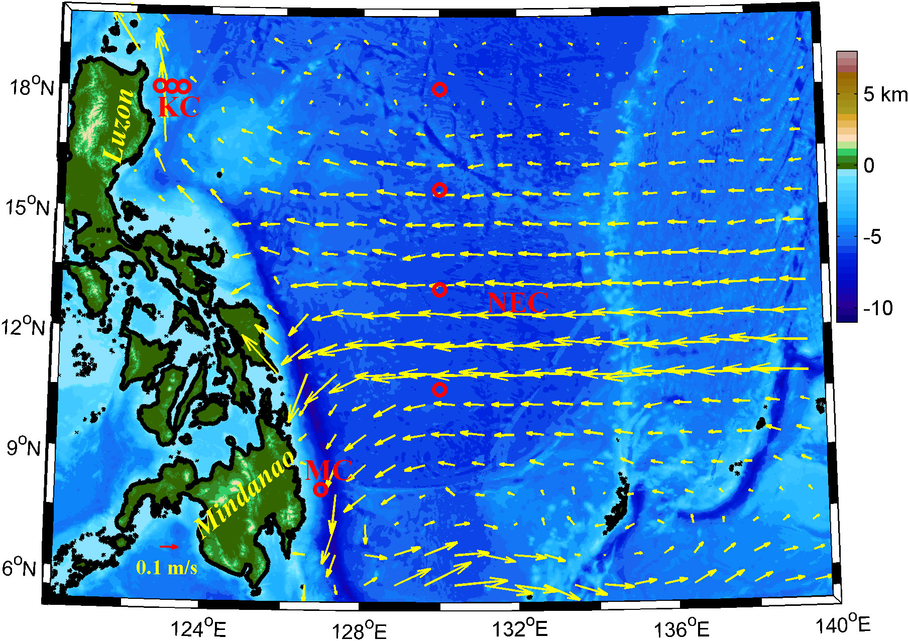
Figure 1 Bottom topography east of the Philippines. Red circles denote moorings at 10.5°N, 13°N, 15.5°N, and 18°N along 130°E; moorings at 122.7°E, 123°E, and 123.3°E along 18°N; and mooring at 127°E/8°N. The arrows represent the mean geostrophic currents from satellite data (1993–2019).

TABLE 1

Table 1 Positions, total days, and corresponding periods for the ADCPs during mooring observations.

The acoustic Doppler current profiler (ADCP) is a system for measuring the vertical profiles of two horizontal velocity components. In our mooring arrays, 75-kHz ADCPs were set to collect data over 60 bins, with 8 m per bin, so that the measurement scope was 480 m. As two ADCPs were fixed at about 450-m depths, each mooring could receive the velocities in the upper 900 m. Thus, the mooring data were suitable for investigating the spatial distribution and temporal variability of the NEUC, LUC, and MUC. The horizontal currents regularly led to a slight slant of the mooring system, so that the real measurement scope was less than that at perpendicular mooring.

All mooring data were subjected to quality control. The ADCP data with a velocity of >2 m/s, inclination angle of >18°, and percent good of<80% were not used. As the echoes of beam emission are strong in the sea surface, the mooring data for the upper 50 m were bad and deleted. Note that the ADCP data at 13°N were good in the upper 50 m. The hourly ADCP data were translated into daily mean to eliminate tidal signals. The mooring data are available at the Marine Science Data Center of the Chinese Academy of Sciences (https://dx.doi.org/10.12157/iocas.2021.0017).

Global sea surface height dataset

The global sea surface height dataset was estimated via optimal interpolation. Measurements from different altimeter missions were merged. The temporal coverage was from January 1993 to December 2019, and the spatial resolution was 0.25° × 0.25°. The satellite dataset was derived from https://marine.copernicus.eu/.

QuikSCAT wind products

The QuikSCAT wind products are produced by the NASA Scatterometer Projects and distributed by the NASA Physical Oceanography Distributed Active Archive Center (PO.DAAC) at the Jet Propulsion Laboratory. QuikSCAT was launched from California’s Vandenberg Air Force Base aboard a Titan II vehicle on 19 June 1999, then a spatially gridded daily wind field map was produced over the global oceans from October 1999 to November 2009 with a spatial resolution of 0.25° × 0.25°. The QuikSCAT wind data can be freely downloaded from http://podaac.jpl.nasa.gov/quikscat.

Results

Mean structure of NKM

Because the KC and MC are almost parallel with the Luzon and Mindanao Island, they can be represented by meridional velocities (Figure 1), while the NEC is described by zonal velocities. In this study, we set northward and eastward as positive. The mean velocities from mooring observation are shown in Figure 2. Generally, the NEC, KC, and MC occur in the upper 500 m. Along 130°E, the maximum mean NEC velocities at 10.5°N, 13°N, 15.5°N, and 18°N are −0.30 m/s (70 m), −0.24 m/s (surface), −0.16 m/s (163 m), and −0.02 m/s (311 m), respectively. Along 18°N, the maximum mean KC values at 122.7°E, 123°E, and 123.3°E are 72.40 cm/s (63 m), 40.61 cm/s (62 m), and 19.52 cm/s (115 m), respectively. At 127°E/8°N, the maximum MC velocity is 78 cm/s at a 100-m depth. The maximum mean KC and MC velocities are higher than the maximum mean NEC velocity, and the cores of the three currents are concentrated in the upper layer. The SSH-derived geostrophic velocity (not shown in the paper) further indicates that the mooring at 122.7°E is close to the maximum velocity of the KC.

FIGURE 2

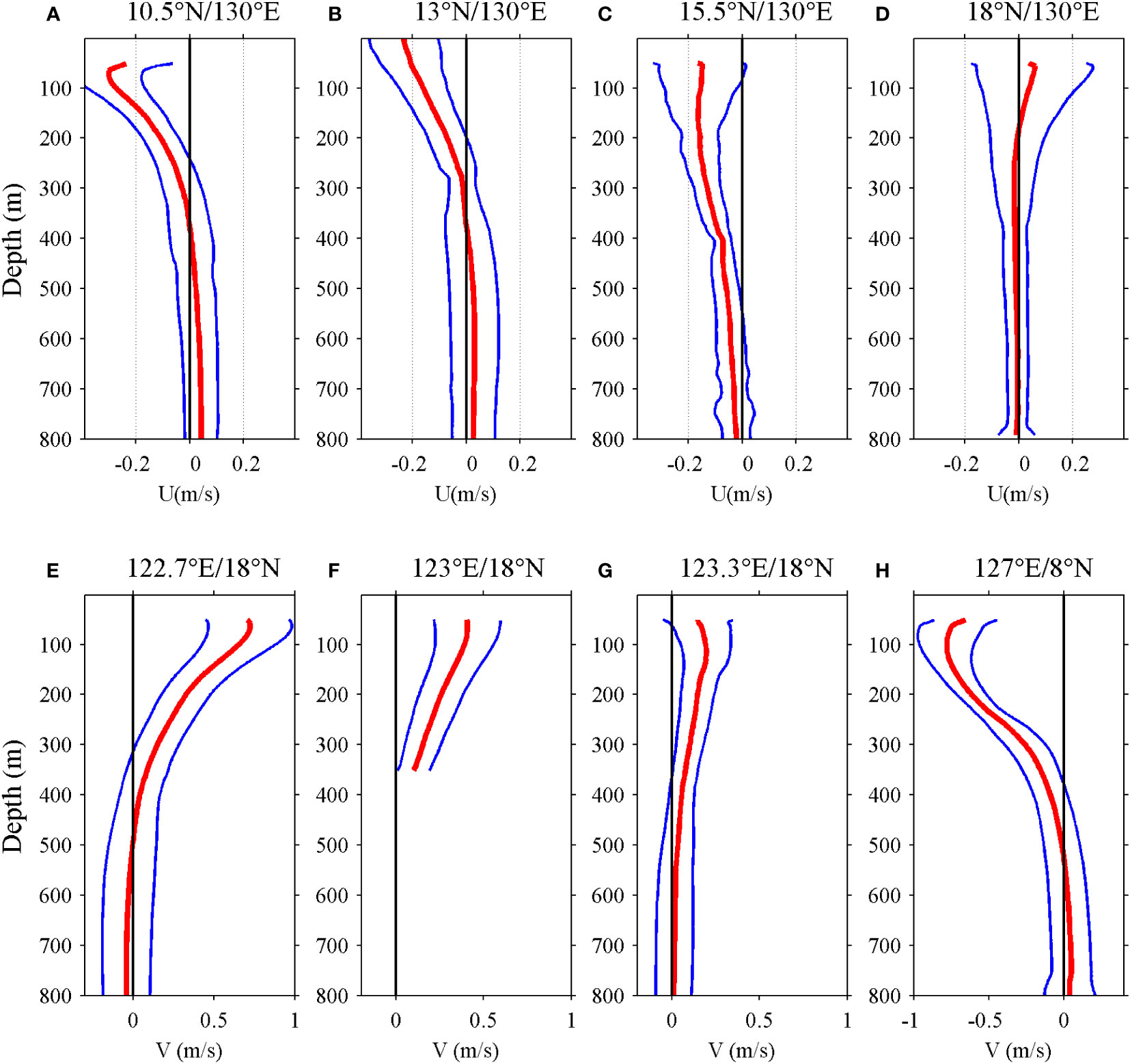
Figure 2 Mean velocities (red lines) and associated standard deviations (blue lines) at (A) 10.5°N, (B) 13°N, (C) 15.5°N, and (D) 18°N along 130°E; (E) 122.7°N, (F) 123°N, (G) 123.3°N along 18°N; and (H) 127°E/18°N. The black line indicates zero velocity. (Units are m/s.).

Along 130°E, the maximum standard deviation of the NEC occurs at 50 m (0.17 m/s), surface (0.21 m/s), 50 m (0.17 m/s), and 59 m (0.22 m/s) at 10.5°N, 13°N, 15.5°N, and 18°N, respectively. At 122.7°E, 123°E, and 123.3°E, the maximum standard deviation of the KC along 18°N is 25.82 cm/s at a depth of 63 m, 18.98 cm/s at 51 m, and 19.90 cm/s at 51 m. At 127°E/8°N, the maximum standard deviation of the MC is 21 cm/s at 59 m. The maximum standard deviations of the three currents are concentrated in the upper 100 m, which suggests that the temporal variability of the NKM is concentrated in the upper layer. In addition, the standard deviations of the three currents are all lower than their means, indicating that the NKM system is stable.

The vertical scales of the KC and MC are larger than that of the NEC, suggesting that the vertical scale of the NKM is a spatial variable instead of a constant. With increasing latitude, the mean NEC decreases, and the vertical scale of the NEC increases. Similar to the NEC, the mean KC decreases and vertically extends with increasing latitude. The NEUC, LUC, and MUC are under the NEC, KC and MC, respectively. Along 130°E, the mean NEUC is significant at 10.5°N and 13°N but disappears at 15.5°N and 18°N, consistent with the results of Qiu et al. (2013). Along 18°N, the mean LUC occurs under 500 m at 18°N/122.7°E and disappears at 18°N/123.3°E. At 127°E/8°N, the mean MUC occurs under 500 at 127°E/8°N.

Seasonal variability of NKM

The seasonal variation in the NKM was investigated using the daily velocities obtained from ADCPs (Figure 3). The NEC velocities at 10.5°N and 13°N are stronger in spring and summer (exceeding 0.4 m/s in April and June) and weaker in autumn. At 15.5°N, the NEC is strong in autumn and weak in spring, which is almost opposite to the cases at 10.5°N and 13°N, indicating that the seasonal phase of the NEC is latitude-dependent. Note that the westward-flowing NEC and the southward-flowing MC are almost negative except at 18°N, since the eastward and northward are set as positive. At 18°N, the direction of meridional velocities changes frequently, suggesting that 18°N is the northern boundary of the NEC.

FIGURE 3

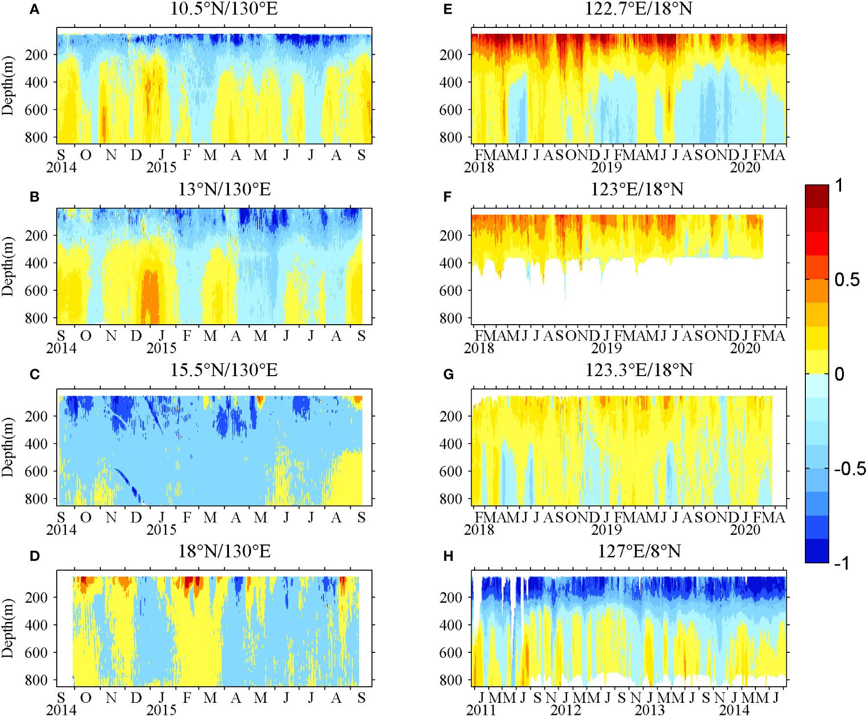
Figure 3 Zonal velocities derived from ADCPs at (A) 10.5°N, (B) 13°N, (C) 15.5°N, (D) 18°N along 130°E and meridional velocities derived from ADCPs at (E) 122.7°E, (F) 123°E, (G) 123.3°E along 18°N and (H) 127°E/8°N. (Units are m/s.).

The maximum KC velocity exceeds 1 m/s, and it decreases eastward from 122.7°E to 123.3°E. Because the eddy activity was strong in 2018, the eddy-induced intraseasonal signals generated a result that the seasonal variability in the KC was not pronounced in 2018. In 2019, the KC was strong in spring and summer and weak in autumn. For the MC, a summer peak occurred in 2011, and spring peaks occurred in 2012, 2013, and 2014, denoting the interannual variation of the MC. The 4-year-averaged mooring data indicate that the MC is strong in spring and summer and weak in autumn. According to the above analysis, the seasonal cycles of the NEC at 10.5°N and 13°N, the KC at 18°N, and the MC at 8°N are almost consistent, although the seasonal phase of the NEC at 15.5°N is almost opposite.

To investigate the intraseasonal variability of the NKM system, the mooring-derived zonal velocities along 130°E and meridional velocities along 18°N and 8°N were processed via power spectrum density (PSD) analysis. The results are presented in Figure 4. At 10.5°N and 13°N, the 70- to 120-day signals are coherent from the surface to 800 m, although the signals are not homogeneous. The maximum signals are located around 400 and 700 m at 10.5°N and 13°N, respectively. At 15.5°N and 18°N, the same-period signals are only concentrated in the upper layer and disappeared in the lower layer. This difference is attributed to thermocline eddies at 10.5°N and 13°N. In addition, the higher frequencies of 30- to 50-day signals are pronounced above 200 m along 130°E, with a northward increase in intensity. At 127°E/8°N, the 60-day coherent peak occupies the whole water column of the mooring measurement. In the upper 150 m, a peak occurred in the 70- to 100-day period signals, and below 500 m, 60- to 80- and 100- to 120-day signals occurred. Along 18°N, significant signals of 50–60 and 80–100 days exist in the upper layers at all three mooring stations. In summary, intraseasonal variability is common in the upper layer of the NKM system. In the lower layer, the existence of intraseasonal signals is location-dependent.

FIGURE 4

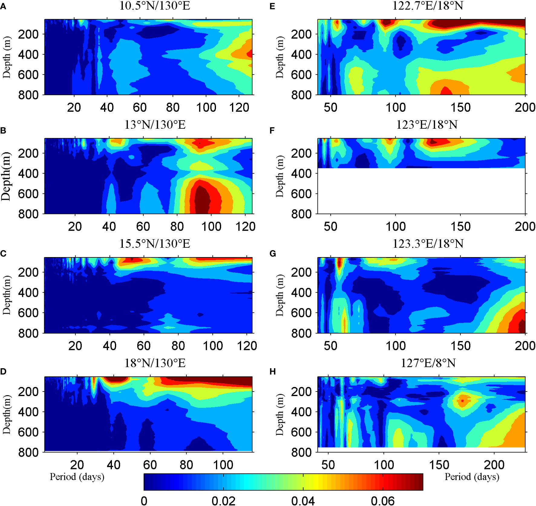
Figure 4 Power spectral density (PSD) of zonal velocities from ADCPs at (A) 10.5°N, (B) 13°N, (C) 15.5°N, (D) 18°N along 130°E and PSD of meridional velocities from ADCPs at (E) 122.7°E, (F) 123°E, and (G) 123.3°E along 18°N and (H) 127°E/8°N. Units are m²/(s² cycles per day [cpd]).

In Figure 3, the daily mean velocities contain too much intraseasonal variability, which masks the seasonal variability, and interannual variability is significant as well compared with seasonal variability (Figure 3H), so it is difficult to capture the exact seasonal variations in the NKM system from Figure 3. The satellite dataset is a good choice because the multiyear monthly means are convenient to remove intraseasonal and interannual variability. In this regard, the purpose of the mooring data is really to provide the accuracy of satellite-based observations given the similarity to satellite-based geostrophic current. Here, satellite data of the same time series (Figure 5) are compared with the mooring observation. The satellite data and mooring observations are not well consistent at 10.5°N/130°E but agree well at the other stations. As depicted in Figure 2, the NEC is surface-intensified, particularly at its southern part; therefore, the inconsistency at 10.5°N/130°E is due to the absence of mooring data for the upper 50 m. At 13°N/130°E, the good data for the upper 50 m result in a much better comparison. Thus, the daily satellite data from 1993 to 2019 are suitable for investigating the seasonal variability and dynamics of the NKM system.

FIGURE 5

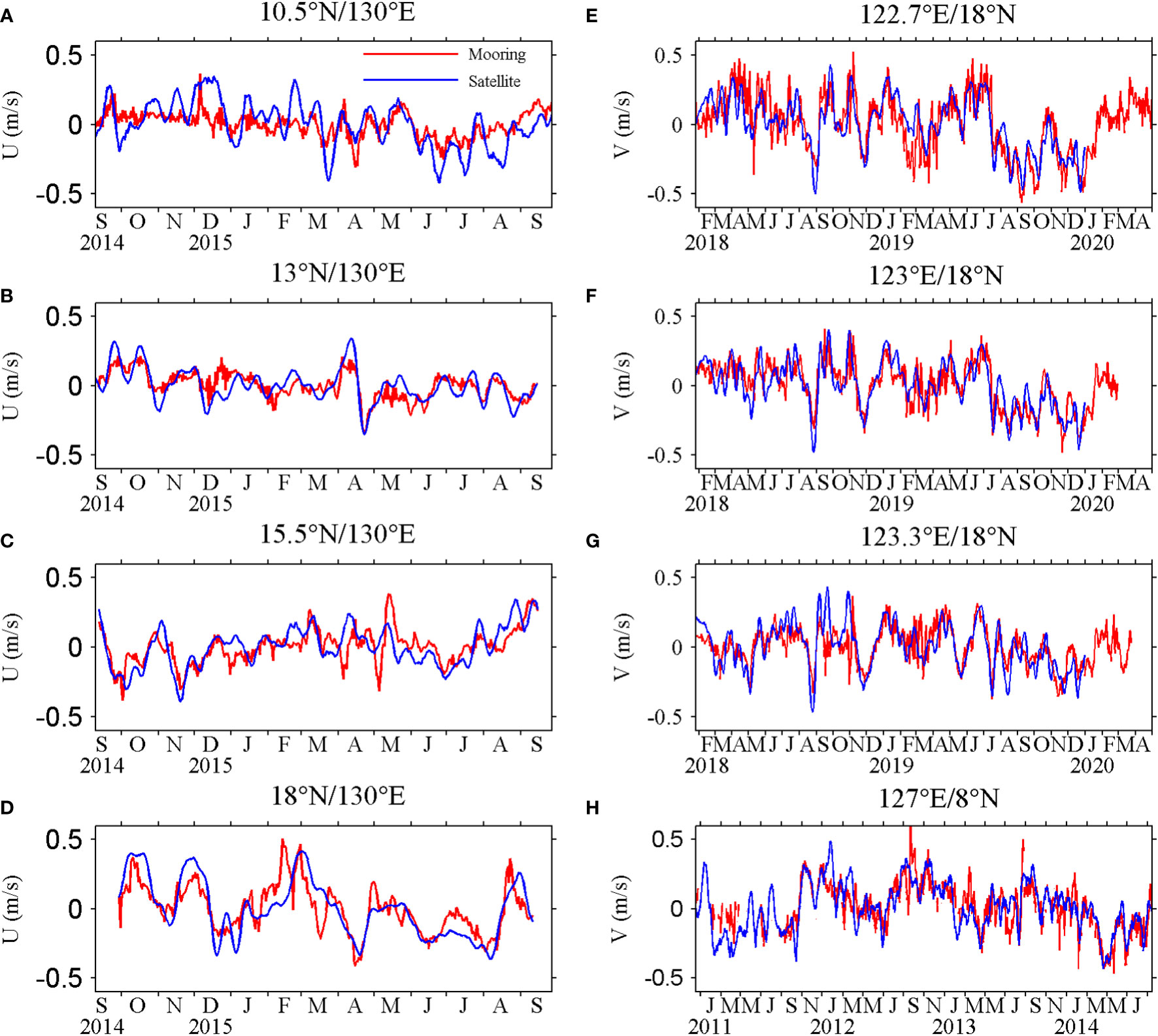
Figure 5 Velocity anomalies from ADCPs (averaged in the upper 150 m) and satellite data during observation period at (A) 10.5°N, (B) 13°N, (C) 15.5°N, and (D) 18°N along 130°E; (E) 122.7°E, (F) 123°E, and (G) 123.3°E along 18°N; and (H) 127°E/8°N. (Units are m/s.).

The monthly mean zonal velocity anomalies along 130°E and the monthly mean meridional velocity anomalies along 18°N and 8°N are depicted in Figure 6. Notice that the stronger/weaker NEC and MC are represented by blue/red colors, as their directions are defined as negative in this study. The seasonal phase of the NEC slightly advances with increasing latitude from 10°N to 14°N and then delays with a further increase in latitude. A double peak of the NEC occurs at 10.5°N, while only one peak occurs at 13°N; thus, the phase advance of the NEC is not significant south of 14°N, resulting in the similarity between the seasonal phases at 10.5°N and 13°N: that is, the current is strongest in spring/summer and weakest in autumn. In the northward continuous delay process, the seasonal phase is reversed at around 16°N, and a peak occurs in both winter and spring at 18°N. As the main body of the NEC is concentrated south of 14°N, the integrated NEC is strongest in spring and weakest in autumn. The KC is strong in winter and spring and weak in autumn, while the MC is maximum in spring and minimum in autumn. The seasonal cycles of the southern part of the NEC, KC, and MC are in phase, although the KC along 18°N has the other peak in winter. The seasonal cycle of the NEC at 18°N is similar to that of the KC, but the seasonal variation of the NEC at 8°N is distinct from that of the MC.

FIGURE 6

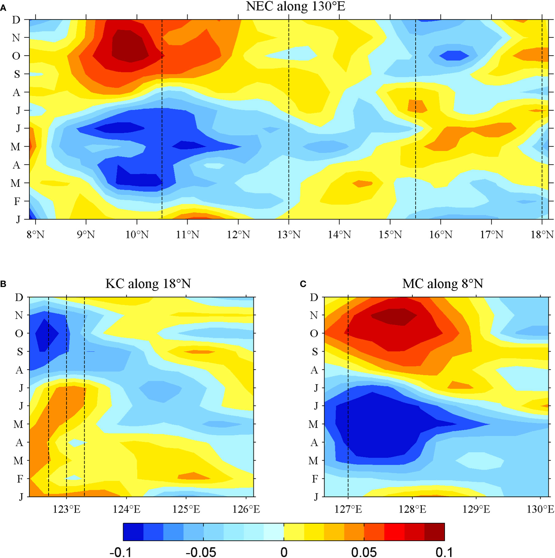
Figure 6 (A) Mean monthly zonal velocity anomalies from satellite data along 130°E and mean monthly meridional velocity anomalies from satellite data (1993–2019) along (B) 18°N and (C) 8°N. (Units are m/s.) The dotted lines represent the location of moorings. Note that the directions of the NEC and MC are opposite to that of the KC.

Dynamics of seasonal variability of NKM

As mentioned above, the main bodies of the three currents could be considered geostrophic flows; therefore, satellite data are suitable for exploring the dynamics. The seasonal sea surface height anomaly (SSHa) west of 140°E is depicted in Figure 7. The arrows represent the corresponding geostrophic currents. A relatively higher/lower SSHa compared with the surrounding area occurs in 123°E–127°E/15°N–20°N during January–May/August–November and occupies the region 127°E–135°E/5°N–10°N in September–December/March–June, respectively. As the main bodies of the KC and MC are located in the western flank of these relatively higher/lower SSHas, the geostrophic relationship indicates that the strong seasons of the KC are winter and spring, while the MC reaches its maximum in spring and summer. Around 15°N, a relatively higher/lower belt occurs in March–June/September–January. The belt induces a westward/eastward flow anomaly in the southern/northern belt area, resulting in different seasonal features of the meridional NEC.

FIGURE 7

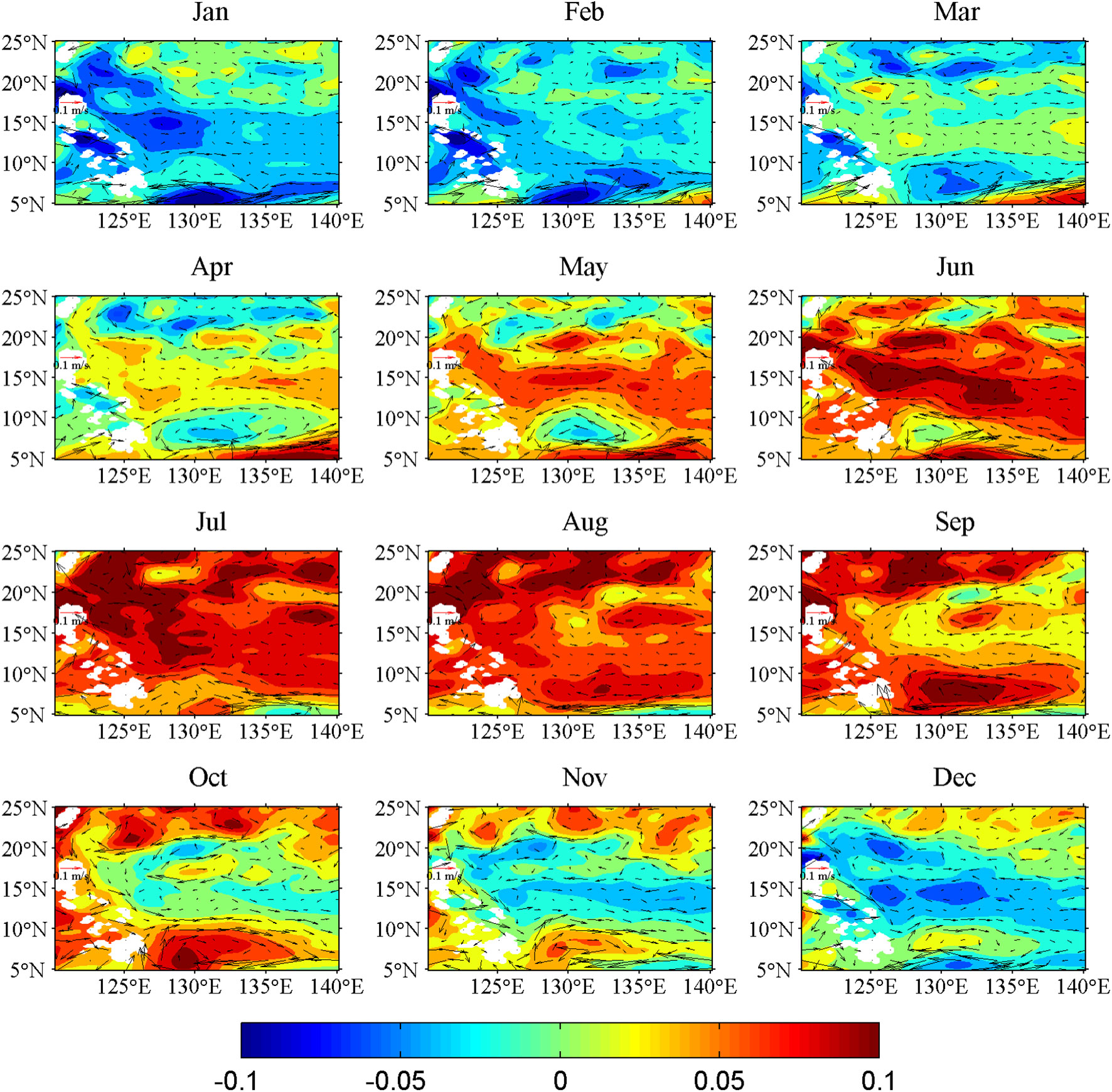
Figure 7 Spatial distribution of seasonal SSHa and associated geostrophic current anomalies (represented by arrows) based on satellite data (1993–2019) east of the Philippines. (Units are m.).

The spatial distribution and temporal variability of SSHa are closely associated with the local wind forcing and westward propagation of Rossby waves (e.g., Qiu and Joyce, 1992; Qiu and Lukas, 1996; Qu et al., 1998). Locally, a positive/negative wind stress curl anomaly will generate a negative/positive SSHa, which will then propagate westward as Rossby waves; therefore, the SSHa at the western boundary can be considered the zonal integration of local and remote effects. To investigate the relative contribution between local wind forcing and Rossby waves, the linearized reduced-gravity equation is used:

$\begin{array}{ll}\frac{\partial h}{\partial t}-\left(\frac{\beta c^2}{f^2}\right)\frac{\partial h}{\partial x}=-\frac{1}{{\rho }_0}\nabla \times \left(\frac{\overrightarrow{\tau }}{f}\right)& (1)\end{array}$

where h(x,y,t) denotes the height deviation from the mean upper layer thickness H₀ $\overrightarrow{\tau }$s the surface wind stress, f s the Coriolis parameter, $\beta =\frac{\partial f}{\partial y}$ $c=\sqrt{g^{\prime }{H}_0}$s the internal wave speed, and $g^{\prime }=\frac{\text{Δ}\rho }{{\rho }_0}g$s the reduced gravity, where ρ₀ nd Δρ denote the seawater density in the upper layer and the density difference between two layers, respectively.

To solve Eq. (1), the mathematical expression of the wind forcing is necessary. Here, we choose the synthetic wind from Qiu and Lukas (1996), which can well describe the zonal mean wind forcing in the North Pacific Ocean.

$\begin{array}{ll}\overrightarrow{k}\mathrm{· }\mathrm{\nabla }\times \overrightarrow{\tau }=-\left\{Acos\left[\omega \left(t-\varphi \right)\right]+B\right\}\sin \left[\frac{2\pi }{L}\left(y-15°+\alpha \cos \omega t\right)\right]& (2)\end{array}$

where y epresents latitude and t = 0 orresponds to January 1. A=0.2[1+0.025(y−7°)]×10⁻⁷N m⁻³ B=3.5A ϕ=60 d, L(y)=40°/(1−0.05(y−15°)) ω=2π/1  year, and α=4° The solution based on Eqs. (1) and (2), as given by Wang et al. (2019), is

$\begin{array}{ll}h\left(x,y,t\right)=a_0\left(x,y\right)+\sum _{n=1}^{\infty }\left\{A_n\left(y\right)sin\left(nk\frac{x}{2}\right)sinnk\left[\frac{x}{2}+c_r\left(y\right)t+{\phi }_n\left(y\right)\right]\right\}& (3)\end{array}$

Where x = 0 s located at the eastern boundary of the North Pacific Ocean, and the propagation speed of baroclinic Rossby waves is expressed as c_r=β c²/f² tan φ_n(y)=a_n(y)/b_n(y) and the wave number is represented by k This solution is valid under the assumption limited by Eq. (2) that the wind stress curl anomaly is longitude-independent.

The monthly mean wind stress curl anomaly is depicted in Figure 8. In the interior ocean, the zero lines are almost parallel with the equator, suggesting that the wind stress curl anomaly is similar in zonal and that the above analytical model is appropriate for analyzing the seasonal variability of the NEC. Figure 9A shows that the seasonal wind stress curl anomaly along 130°E between 15°N and 20°N is almost the same in meridional; therefore, the meridional phase difference in the SSHa reduces to c_rt because the φ_n(y) in Eq. (3) is negligible in this region. The poleward decrease in the propagation speed of the Rossby waves results in northward delays in the seasonal phase of NEC, consistent with the results in Figure 6. The northward delay process generates a reversed seasonal cycle of NEC at 15.5°N, and the seasonal variation at 18°N is similar to those at 10.5°N and 13°N. Because the meridional gradient of the propagation speed of Rossby waves decreases poleward (Chelton et al., 1998), the northward delay process of SSHa is not homogeneous but becomes slower, and its meridional gradient attenuates at a higher latitude, indicating that the seasonal NEC weakens with increasing latitude north of 15°N.

FIGURE 8

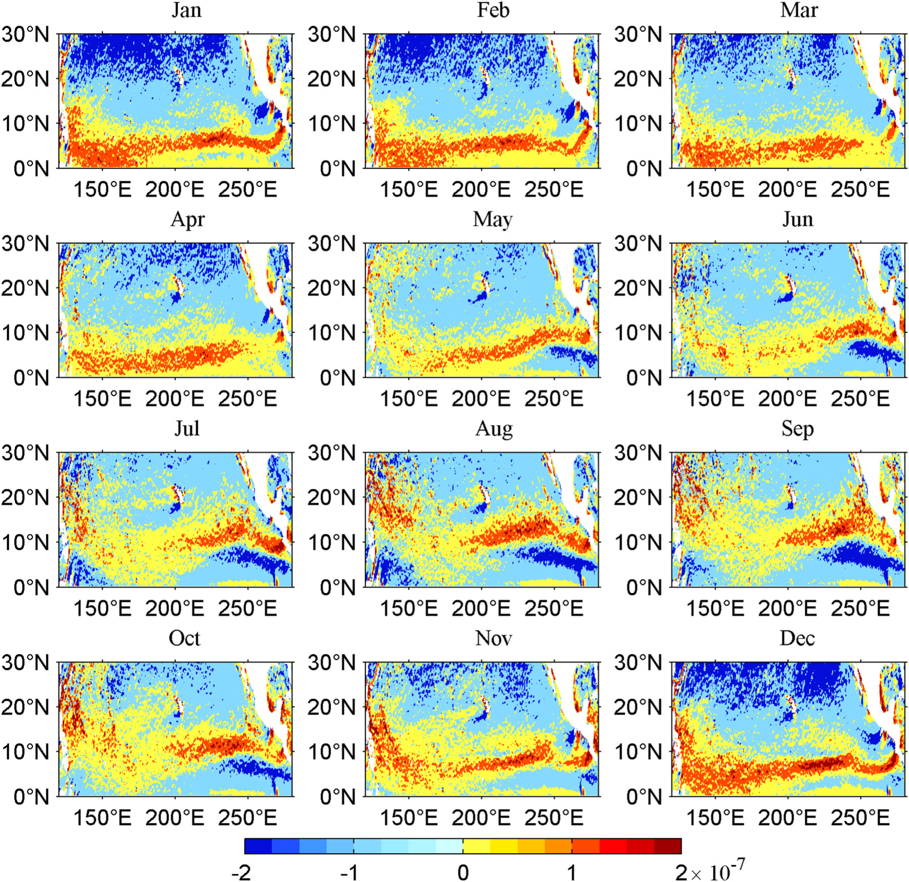
Figure 8 Spatial distribution of seasonal wind stress curl anomalies based on QuikSCAT products (1999–2009) in the North Pacific Ocean. (Units are 10⁻⁷ N m⁻³.).

FIGURE 9

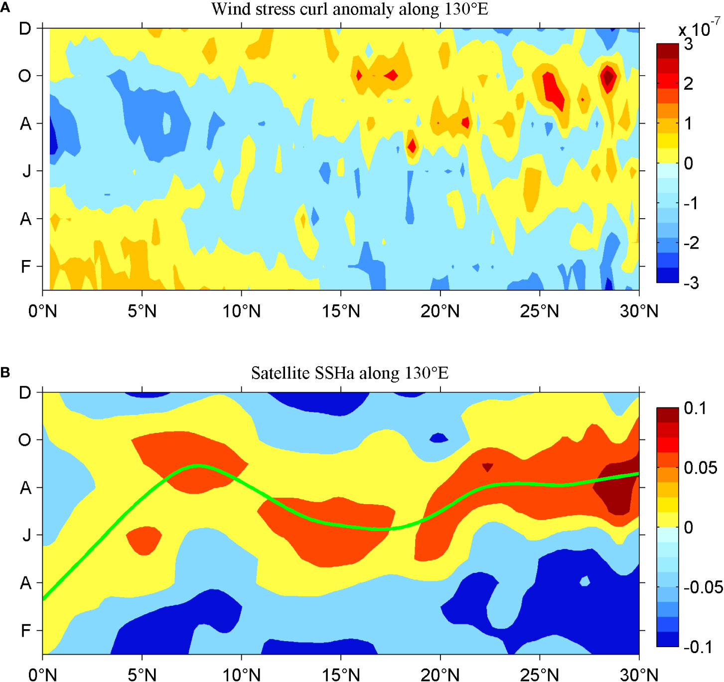
Figure 9 (A) Latitude–time diagram of seasonal wind stress curl anomaly along 130°E based on QuikSCAT products (1999–2009) (units are 10⁻⁷ N m⁻³), and (B) latitude–time diagram of seasonal SSHa from satellite data (1993–2019) along 130°E (units are m). The green line denotes the maximum SSHa in the continuous positive belt of the SSHa in meridional.

As shown in Figure 9A, the phase advance of wind forcing from 7°N to 15°N along 130°E is significant; therefore, φ_n(y) cannot be neglected in this belt, and directly investigating the seasonal phase using Eq. (3) is difficult. The phase advance of SSHa is also pronounced from 7°N to 15°N along 130°E (Figure 9B), which indicates that the local wind forcing plays a dominant role in the south 15°N along 130°E. The phase advance of SSHa south of 15°N is steeper than the delay process north of 15°N, suggesting that the meridional gradients of SSHa and the associated NEC south of 15°N are stronger than those north of 15°N, consistent with the results in Figure 6.

Because the wind stress curl anomaly varies zonally in the western boundary (Figure 8), the solution based on Eq. (2) is not suitable for describing the seasonal features of the KC and MC. To quantitatively investigate the local wind, the propagation term $\left(\frac{\beta c^2}{f^2}\right)\frac{\partial h}{\partial x}$ in Eq. (1) is neglected, and then the wind-driven SSHa is derived under the transformation$\eta =\frac{g^{\prime }}{g}h$

$\begin{array}{ll}\eta \left(x,y,t\right)=-\underset{t_0}{\overset{t}{\int }}\frac{g^{\prime }}{g{\rho }_{0}f}\left(k·\nabla \times {\tau }_a+\frac{\beta }{f}{\tau }_{ax}\right)dt& (4)\end{array}$

where η(x,y,t) depicts SSHa and $\nabla =\frac{\partial }{\partial x}i+\frac{\partial }{\partial y}j$ 〈i,j〉 represents eastward and northward; τ_a denotes the wind stress anomaly. $\frac{g^{\prime }}{g}=\frac{\text{Δ}\rho }{{\rho }_0}$ demonstrates ocean stratification. Here, we set $\frac{\text{Δ}\rho }{{\rho }_0}\approx 0.003$The satellite SSHa and the local wind-driven SSHa along 8°N derived from Eq. (4) are depicted in Figure 10. As shown in Figures 10A, B, the Rossby waves propagate westward from the eastern boundary, and the maximum/minimum arrives around 130°E in September/March. SSHa propagates eastward from the western boundary to 130°E. Furthermore, the propagation speed of SSHa between 130°E and 140°E is lower than that east of 140°E (Figure 10B), which is inconsistent with the results of Chelton et al. (1998), who found that the propagation speed of Rossby waves was larger toward the west. Thus, the local wind forcing is important and cannot be neglected west of 140°E along 8°N. As shown in Figure 10C, around 127.1°E, a maximum exists in spring and a minimum occurs in autumn. Between 131°E and 135°E, it is almost reversed with that around 127.1°E. This reversed process generates a westward phase advance/eastward propagation of wind-driven SSHa from 127°E to 135°E. As mentioned above, the satellite-derived SSHa propagates eastward from the western boundary to 130°E. This indicates that the local wind plays a dominant role west of 130°E. Between 130°E and 135°E, the satellite SSHa propagates slowly westward, owing to the eastward propagation of wind-driven SSHa and the westward propagation of Rossby waves. In the interior ocean between 135°E and 220°E, the seasonal phase is almost opposite to that between 131°E and 135°E but similar to that around 127.1°E (Figure 10D). The conflicting process (i.e., the near-opposite phases between 135°E–220°E and 131°E–135°E) results in a slow westward phase delay of SSHa, and consequently, the wind-driven SSHa propagates slowly toward the west from 140°E to 130°E. The lower propagation speed of the local wind-driven SSHa and the higher speed of the westward Rossby waves result in a slower westward propagation of the satellite SSHa from 140°E to 130°E, consistent with the results in Figure 10B. When the SSHa signals arrive at 140°E, the SSHa westward propagation will slow down between 130°E and 140°E and stop at around 130°E, owing to the local wind effect. Thus, the local wind is dominant west of 130°E and plays an important role between 130°E and 140°E. The SSHas forced by the wind stress curl anomaly and the zonal wind stress anomaly along 8°N are depicted in Figures 10E–H and, respectively. The former is larger than the latter; therefore, the wind stress curl anomaly is more important than the zonal wind stress anomaly along 8°N in Eq. (4).

FIGURE 10

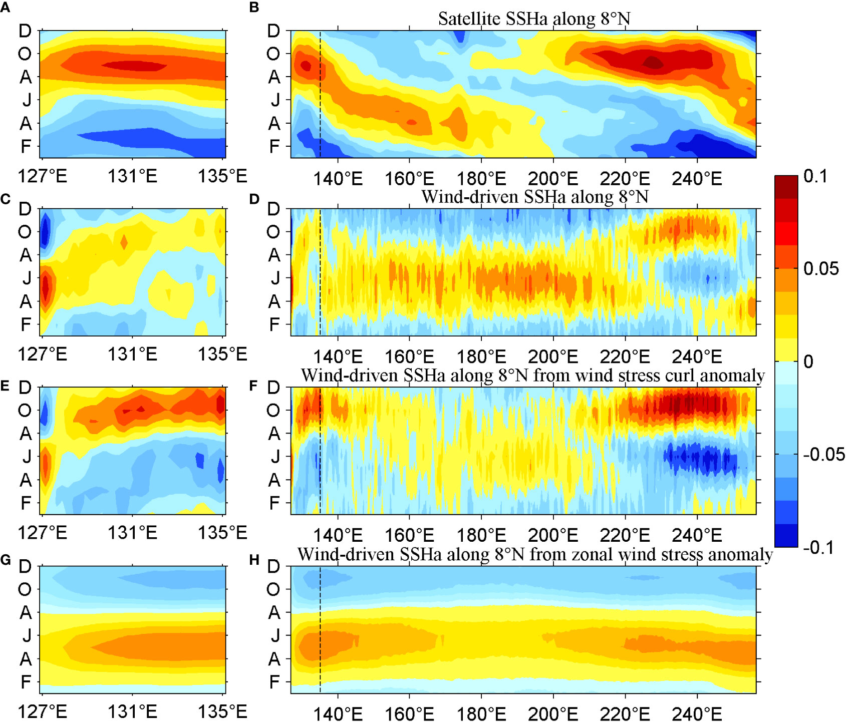
Figure 10 Longitude–time diagrams of seasonal SSHa along 8°N from satellite data (1993–2019) (A) along the western boundary and (B) in the North Pacific Ocean. Diagrams of wind-driven SSHa along 8°N based on QuikSCAT products (1999–2009) calculated from Eq. (4) (C) along the western boundary and (D) in the North Pacific Ocean. Diagrams of wind-driven SSHa along 8°N based on QuikSCAT products (1999–2009) forced by wind stress curl anomaly (E) along the western boundary and (F) in the North Pacific Ocean, and by zonal wind stress anomaly (G) along the western boundary and (H) in the North Pacific Ocean. (Units are m.).

The wind stress curl anomaly along 8°N (Figure 11A) features a comparable reverse process to the wind-forced SSHa (Figure 10D). This confirms that the spatial and temporal variabilities of wind-driven SSHa are mainly determined by that of the wind stress curl anomaly along 8°N at the western boundary. The local wind-driven meridional flow anomaly is calculated (Figure 11B) to be strongest in spring and weakest in autumn, and its core is distributed between 127°E and 128°E, consistent with the results from satellite data (Figure 6C). The wind-forced MC is considerably larger than the observation, which suggests that the Rossby waves, non-linearity, and other factors attenuate the wind-driven MC.

FIGURE 11

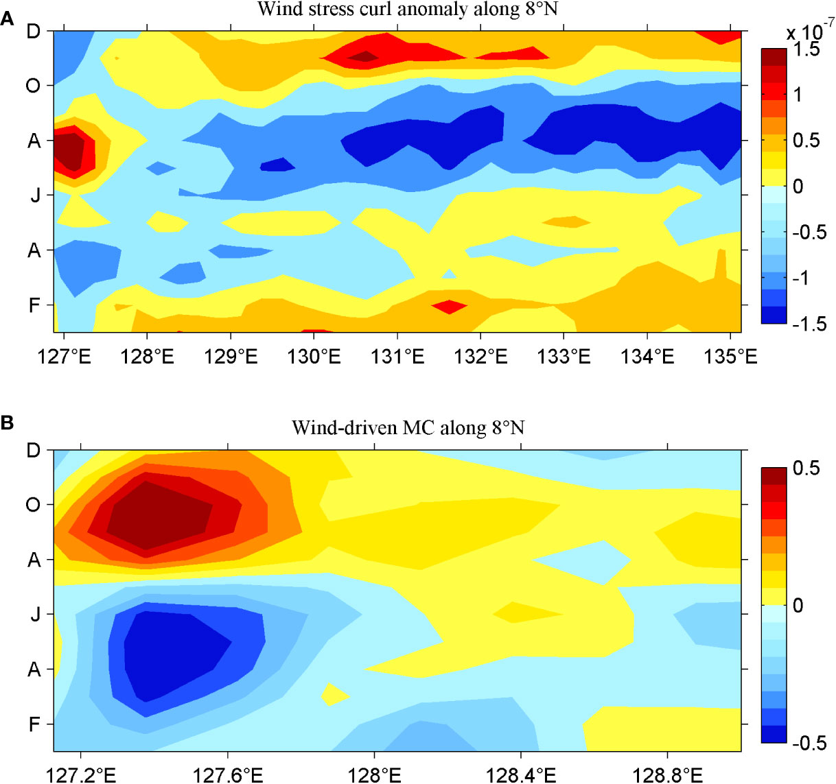
Figure 11 (A) Longitude–time diagram of seasonal wind stress curl anomaly along 8°N based on QuikSCAT products (1999–2009) (units are 10⁻⁷ N m⁻³), and (B) associated longitude–time diagram of seasonal wind-driven MC along 8°N (units are m/s).

As shown in Figures 12A, B the spatial distribution of satellite SSHa along 18°N west of the dateline is quite different from that in the east side, and the westward intensification is pronounced west of the dateline. This indicates that the local wind plays an important role in the KC region. The local wind-driven SSHa along 18°N, calculated from Eq. (4), is depicted in Figures 12C, D. The wind-driven SSHa along 18°N is smaller than that along 8°N, owing to the inverse relationship between η and f n Eq. (4). East of 122.8°E, the wind-driven SSHa is positive from February to August and negative in the remaining months. The similar zonal phase indicates that there is almost no propagation of the wind-driven SSHa along 18°N in the interior ocean. West of 122.6°E, the seasonal phase is reversed, which results in the generation of a large zonal gradient of wind-driven SSHa and an associated meridional current anomaly. As shown in Figure 13A, the calculated wind-driven KC is strongest in spring and weakest in autumn, and its variability mainly occurs west of 123°E, consistent with the seasonal KC from satellite data (Figure 6B). Similar to the wind-driven MC, the wind-driven KC velocity is higher than the satellite data, owing to the adjustment from Rossby waves, non-linearity, and other factors. In addition, the SSHas along 18°N forced by wind stress curl anomaly and zonal wind stress anomaly are shown in Figures 12E–H respectively. Similar to the case along 8°N, the wind stress curl anomaly term is larger than the zonal wind stress anomaly term. The degree of similarity between Figures 13D, F is higher than that between Figures 10D, F, indicating that the relative contribution from wind stress curl anomaly term along 18°N is larger than that along 8°N; thus, the relative contribution from wind stress curl anomaly term increases poleward, which is expected, considering that the Coriolis parameter is in the denominator of the zonal wind stress term in Eq. (4).

FIGURE 12

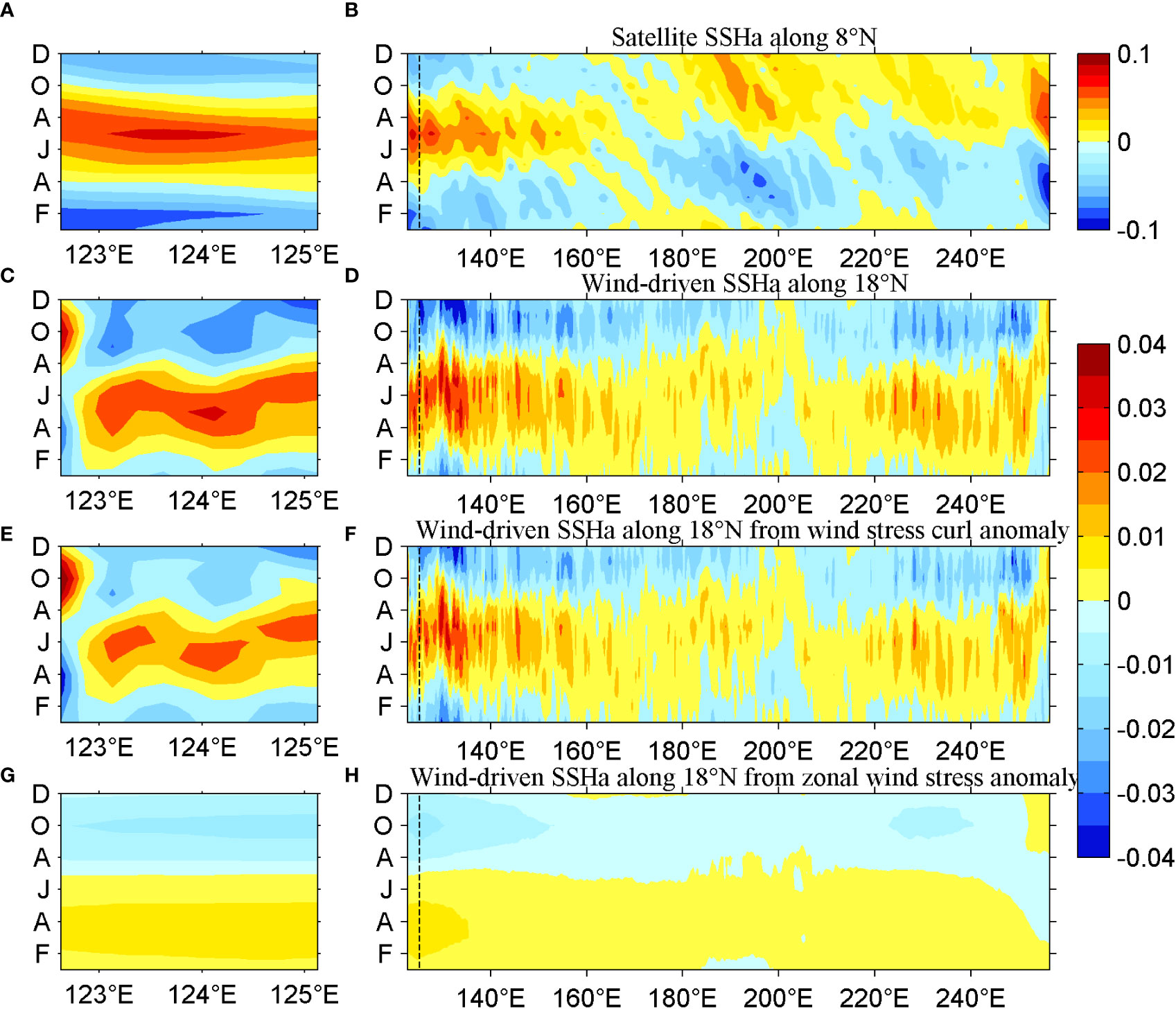
Figure 12 Longitude–time diagrams of seasonal SSHa along 18°N from satellite data (1993–2019) (A) along the western boundary and (B) in the North Pacific Ocean. Diagrams of wind-driven SSHa along 18°N based on QuikSCAT products (1999–2009) calculated from Eq. (4) (C) along the western boundary and (D) in the North Pacific Ocean. Diagrams of wind-driven SSHa along 18°N based on QuikSCAT products (1999–2009) forced by wind stress curl anomaly (E) along the western boundary and (F) in the North Pacific Ocean, and by zonal wind stress anomaly (G) along the western boundary and (H) in the North Pacific Ocean. (Units are m.).

FIGURE 13

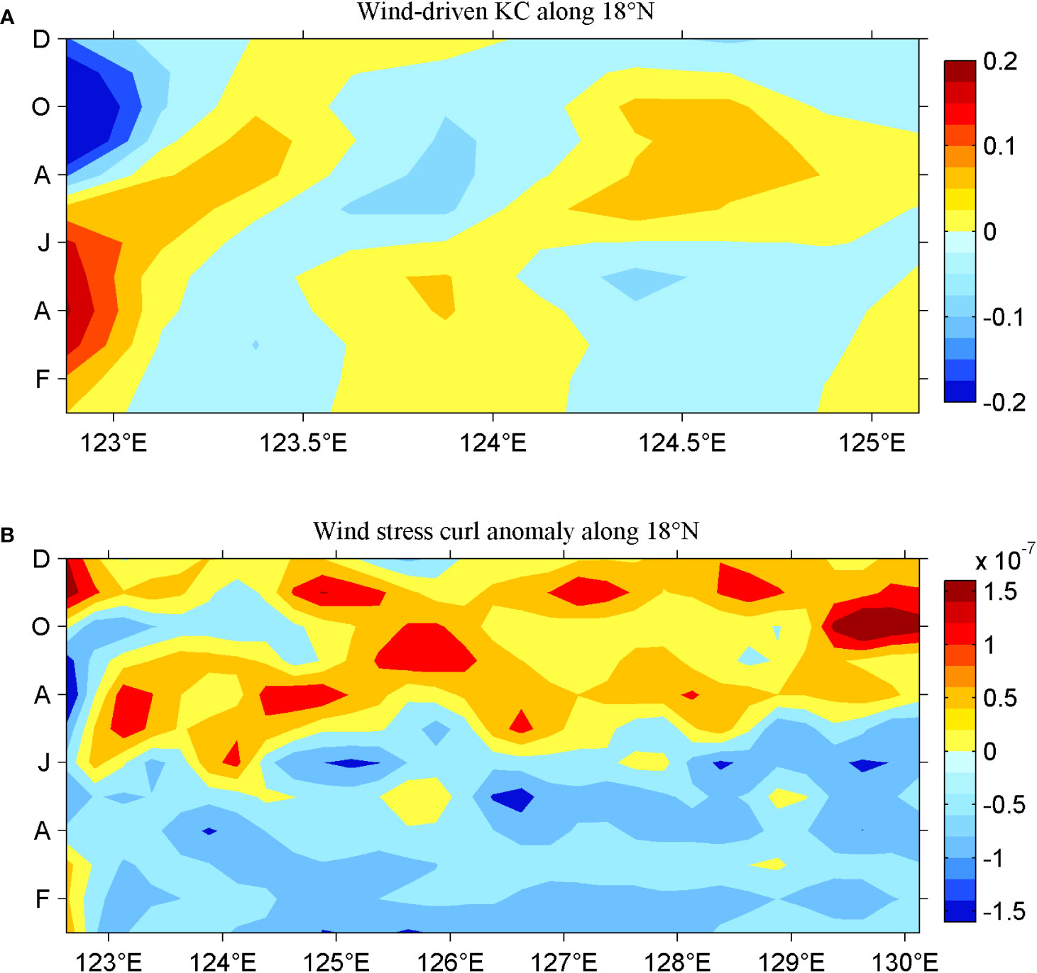
Figure 13 (A) Longitude–time diagram of seasonal wind-driven KC along 18°N (units are m/s), and (B) longitude–time diagram of seasonal wind stress curl anomaly along 18°N based on QuikSCAT products (1999-2009) (units are 10⁻⁷ N m⁻³).

The wind stress curl anomaly along 18°N is shown in Figure 13B. Generally, the negative/positive wind stress curl anomaly occupies east of 122.8°E in the first/second half of the year. In comparison, the seasonal phase is almost reversed west of 122.6°E, resulting in the generation of a large zonal gradient of wind-driven SSHa and associated variability of KC. The seasonal phase of wind forcing is not well consistent with that of the wind-driven SSHa, as the latter is derived by the integration of the former according to Eq. (4). Interestingly, the longitude–time diagram of the wind stress curl anomaly at the western boundary along 18°N (Figure 13B) is almost opposite to that along 8°N (Figure 11A); consequently, the northward KC and the southward MC exhibit similar seasonal variation.

Conclusion and discussion

Utilizing the direct mooring observations along 130°E, 18°N, and 8°N and satellite data, the seasonal variability and dynamics of the NKM are discussed. Three currents were generally located in the upper 500 m, and the vertical depths of the KC and MC were greater than that of the NEC. The NKM system was stable, as the standard deviations of the three currents were less than their means. The maximum standard deviations of the three currents were concentrated in the upper 100 m, indicating that the variability of the NKM was concentrated in the upper layer. The PSD analysis revealed that the intraseasonal signals of the NKM were common in the upper layer. Zhang et al. (2017) revealed that the vertical structure of intraseasonal variability along 130°E varied with latitude. Wang et al. (2022) indicated that the atypical seasonal variability of the KC in 2018 was due to the strong intraseasonal signals generated by eddy activity. Along 8°N, subthermocline eddies translated westward and intensified near the Mindanao coast, generating intraseasonal signals over 60–80 days at 127°E/8°N (Zhang et al., 2014).

The seasonal variability of the three currents was investigated using mooring and satellite data (Zhang L. et al., 2021). The MC along 8°N was strongest in spring and weakest in autumn. Qu et al. (2008) showed that the ratio of the semiannual to annual variation at 100 m was ~0.8 at 6°50′N/126°43′E. The annual signals were more than 6 cm from 5°N to 10°N along the western boundary, while the semiannual variation was confined within about 5° of the equator. At our mooring station 127°E/8°N, the ratio reduced to about 2 to 6; thus, the semiannual signals were significant (Figure 4H) but not stronger than the annual signals at 127°E/8°N. The KC along 18°N was maximum in winter and spring and minimum in autumn. Interestingly, the seasonal NEC was latitude-dependent. Along 130°E, it was stronger in spring and weaker in autumn at 10°N; then, the seasonal phase slightly advanced from 10°N to 14°N and delayed northward. Around 16°N, the maximum NEC occurred in autumn, and a peak existed in both winter and spring at 18°N. Because the main body of the NEC was located south of 14°N and was maximum/minimum in spring/autumn, the seasonal phase of the three currents was generally in phase, while the KC featured another peak in winter.

The seasonal variability of the NKM system was closely associated with the local wind and Rossby waves. The positive/negative local wind stress curl anomaly generated a negative/positive SSHa and an associated anticyclonic/cyclonic flow anomaly. The wind-forced SSHa propagates toward the west as Rossby waves (e.g., Qiu and Lukas, 1996; Qu et al., 1998). Thus, the observed SSHa can be considered the results of local winds and Rossby waves. Because the velocities derived from mooring observations along 130°E, 18°N, and 8°N were consistent with those derived from satellite data, the effects of non-linearity and the friction term were much smaller than the effects of the local wind and Rossby waves. Lien et al. (2014) indicated that the geostrophic relationship well describes the KC, except for the upper 100 m of the western flank of the KC.

Along 130°E, the seasonal phase of SSHa from satellite data was latitude-dependent. It delayed from the equator to 7°N and from 15°N to 30°N but advanced from 7°N to 15°N. In comparison, the seasonal phase of the wind stress curl anomaly advanced from the equator to 30°N. The phase similarity between local wind and SSHa from 7°N to 15°N indicates that the local wind was dominant in this region. North of 15°N, the out-of-phase relationship between the local wind and SSHa denotes that the Rossby waves played an important role in the northern part of the NEC. Similar to the seasonal variation, Huang et al. (2022) reported that the phase of the interannual variation of the NEC delayed with increasing latitude, with the signal at 15°N lagging that at 8.5°N by about 1 year. The NEC was strengthened with the weakening NEUC, and the NEUC at 8.5°N was intensified during the mature phase of El Niño and reached its maximum during the decay phase of El Niño.

The wind stress curl anomaly behaviors along 8°N and 18°N were similar; that is, the seasonal phase along the western boundary was opposite to that located farther away in the east. This resulted in the generation of a strong gradient of wind-driven SSHa and an associated current anomaly on the western boundary. A comparison of the mooring and satellite data revealed that the local wind-forced meridional flow anomalies along 8°N and 18°N well reproduced the seasonal phases of the MC and KC, indicating that the local wind played a dominant role in the seasonal variability of the MC and KC. In addition, the wind-forced currents were both larger than the observation, attributable to the adjustment of the Rossby waves and other factors, such as nonlinearity and friction.

In summary, the seasonal variabilities in the southern part of the NEC along 130°E, the KC along 18°N, and the MC along 8°N were similar. In the northern part of the NEC along 130°E, the seasonal cycle delayed with increasing latitude. In the zonal NKM, the local wind played a dominant role in the seasonal variability of the KC and MC via a geostrophic relationship. The seasonal cycle of the meridional NEC was mainly controlled by local/remote effects in the southern/northern part.

Data availability statement

The original contributions presented in the study are included in the article/supplementary material. Further inquiries can be directed to the corresponding author.

Author contributions

FW proposed the main ideas and wrote sections of the manuscript. LZ performed the data analysis and modified the manuscript. JF and DH participated in the discussion and contributed to the improvement of the manuscript. All authors contributed to the article and approved the submitted version.

Funding

This research was funded by the Strategic Priority Research Program of the Chinese Academy of Sciences (grant XDB42010105), the Financially supported by Marine S&T Fund of Shandong Province for Pilot National Laboratory for Marine Science and Technology (Qingdao) (grant 2022QNLM010203), and the National Key Research and Development Program of China (No. 2020YFA0608801). Mooring data were collected onboard of R/V KeXue implementing the open research cruise NORC2021-09 supported by the NSFC Shiptime Sharing Project (Grant No. 42049909).

Acknowledgments

We express our sincere gratitude to all scientists and technicians on R/V Science and Science 3 for the deployment and retrieval of the subsurface moorings used in this work.

Conflict of interest

The authors declare that the research was conducted in the absence of any commercial or financial relationships that could be construed as a potential conflict of interest.

Publisher’s note

All claims expressed in this article are solely those of the authors and do not necessarily represent those of their affiliated organizations, or those of the publisher, the editors and the reviewers. Any product that may be evaluated in this article, or claim that may be made by its manufacturer, is not guaranteed or endorsed by the publisher.

References

Chao S. Y. (1991). Circulation of the East China Sea, a numerical study. J. Oceanogr. 46, 273–295. doi: 10.1007/BF02123503

CrossRef Full Text | Google Scholar

Chelton D. B., deSzoeke R. A., Schlax M. G., Naggar K. E., Siwertz N. (1998). Geographical variability of the first-baroclinic rossby radius of deformation. J. Phys. Oceanogr. 28, 433–460. doi: 10.1175/1520-0485(1998)028<0433:GVOTFB>2.0.CO;2

CrossRef Full Text | Google Scholar

Chen Z., Wu L., Qiu B., Li L., Hu D., Liu C., et al. (2015). Strengthening kuroshio observed at its origin during November 2010 to October 2012. J. Geophys. Res. 120, 2460–2470. doi: 10.1002/2014JC010590

CrossRef Full Text | Google Scholar

Donguy J. R., Meyers G. (1996). Mean annual variation of transport of major current in the tropical pacific ocean. Deep-Sea Res. I. 43, 1105–1122. doi: 10.1016/0967-0637(96)00047-7

CrossRef Full Text | Google Scholar

Ffield A., Gordon A. L. (1992). Vertical mixing in the Indonesian thermocline. J. Phys. Oceanogr. 22, 184–195. doi: 10.1175/1520-0485(1992)022<0184:VMITIT>2.0.CO;2

CrossRef Full Text | Google Scholar

Gordon A. L., Flament P., Villanoy C., Centurioni L. (2014). The nascent kuroshio of lamon bay. J. Geophys. Res. 119, 4251–4263. doi: 10.1002/2014JC009882

CrossRef Full Text | Google Scholar

Huang Y., Zhang L., Wang F., Wang F., Hu D. (2022). Interannual variations of the north equatorial Current/Undercurrent from mooring array observations. Front. Mar. Sci. 9. doi: 10.3389/fmars.2022.979442

PubMed Abstract | CrossRef Full Text | Google Scholar

Hu D., Cui M. (1991). The western boundary current of the pacific and its role in the climate. J. Oceanol. Limnol. 9, 1–14. doi: 10.1007/BF02849784

CrossRef Full Text | Google Scholar

Hu D., Wu L., Cai W., Sen Gupta A., Ganachaud A., Qiu B., et al. (2015). Pacific western boundary currents and their roles in climate. Nature 522, 299–308. doi: 10.1038/nature14504

PubMed Abstract | CrossRef Full Text | Google Scholar

Joyce T., Yasuda I., Hiroe Y., Komatsu K., Kawasaki K., Bahr F. (2001). Mixing in the meandering kuroshio extension and the formation of north pacific intermediate water. J. Geophys. Res. 106, 4397–4404. doi: 10.1029/2000JC000232

CrossRef Full Text | Google Scholar

Kashino Y., Ishida A., Kuroda Y. (2005). Variability of the Mindanao current: mooring observation results. Geophys. Res. Lett. 32, L18611. doi: 10.1029/2005GL023880

CrossRef Full Text | Google Scholar

Lien R. C., Ma B., Cheng Y. H., Ho C. R., Qiu B., Lee C. M., et al. (2014). Modulation of kuroshio transport by mesoscale eddies at the Luzon strait entrance. J. Geophys. Res. 119, 2129–2142. doi: 10.1002/2013JC009548

CrossRef Full Text | Google Scholar

Lien R. C., Ma B., Lee C. M., Sanford T. B., Mensah V., Centurioni L. R., et al. (2015). The kuroshio and Luzon undercurrent east of Luzon island. Oceanography 28, 54–63. doi: 10.5670/oceanog.2015.81

CrossRef Full Text | Google Scholar

Lukas R., Firing E., Hacker P., Richardson P., Collins C., Fine R., et al. (1991). Observations of the Mindanao current during the Western equatorial pacific ocean circulation study. J. Geophys. Res. 96, 7089–7104. doi: 10.1029/91JC00062

CrossRef Full Text | Google Scholar

Nakano H., Tsujino H., Sakamoto K. (2013). Tracer transport in cold-core rings pinched off from the kuroshio extension in an eddy-resolving ocean general circulation model. J. Geophys. Res. 118, 5461–5488. doi: 10.1002/jgrc.20375

CrossRef Full Text | Google Scholar

Nitani H. (1972). “Beginning of the kuroshio,” in Kuroshio: Its physical aspects. Eds. Stommel H., Yoshida K. (Seattle: Univ. of Wash. Press), 129–163.

Google Scholar

Qiu B., Chen S., Schneider N. (2017). Dynamical links between the decadal variability of the oyashio and kuroshio extensions. J. Climate. 30, 9591–9605. doi: 10.1175/JCLI-D-17-0397.1

CrossRef Full Text | Google Scholar

Qiu B., Chen S., Schneider N., Taguchi B. (2014). A coupled decadal prediction of the dynamic state of the kuroshio extension system. J. Climate. 27, 1751–1764. doi: 10.1175/JCLI-D-13-00318.1

CrossRef Full Text | Google Scholar

Qiu B., Joyce T. M. (1992). Interannual variability in the mid- and low-latitude western north pacific. J. Phys. Oceanogr. 22, 1062–1084. doi: 10.1175/1520-0485(1992)022<1062:IVITMA>2.0.CO;2

CrossRef Full Text | Google Scholar

Qiu B., Lukas R. (1996). Seasonal and interannual variability of the north equatorial current, the Mindanao current, and the kuroshio along the pacific western boundary. J. Geophys. Res. 101, 12315–12330. doi: 10.1029/95JC03204

CrossRef Full Text | Google Scholar

Qiu B., Rudnick D. L., Cerovecki I., Cornuelle B. D., Chen S., Schönau M. C., et al. (2015). The pacific north equatorial current: New insights from the origins of the kuroshio and Mindanao currents (OKMC) project. Oceanography 28, 24–33. doi: 10.5670/oceanog.2015.78

CrossRef Full Text | Google Scholar

Qiu B., Rudnick D., Chen S., Kashino Y. (2013). Quasi-stationary north equatorial undercurrent jets across the tropical north pacific ocean. Geophys. Res. Lett. 40, 2183–2187. doi: 10.1002/grl.50394

CrossRef Full Text | Google Scholar

Qu T. (2001). Role of ocean dynamics in determining the mean seasonal cycle of the south China Sea surface temperature. J. Geophys. Res. 106, 6943–6955. doi: 10.1029/2000JC00479

CrossRef Full Text | Google Scholar

Qu T., Gan J., Ishida A., Kashino Y., Tozuka T. (2008). Semiannual variation in the western tropical pacific ocean. Geophys.Res. Lett. 35, L16602. doi: 10.1029/2008GL035058

CrossRef Full Text | Google Scholar

Qu T., Mitsudera H., Yamagata T. (1998). On the western boundary currents in the Philippine Sea. J. Geophys. Res. 103, 7537–7548. doi: 10.1029/98JC00263

CrossRef Full Text | Google Scholar

Qu T., Song Y., Yamagata T. (2009). An introduction to the south China Sea throughflow: Its dynamics, variability, and application for climate. Dynam. Atmos. Oceans. 47, 3–14. doi: 10.1016/j.dynatmoce.2008.05.001

CrossRef Full Text | Google Scholar

Sasaki Y., Minobe S. (2015). Climatological mean features and interannual to decadal variability of ring formations in the kuroshio extension region. J. Oceanogr. 71, 499–509. doi: 10.1007/s10872-014-0270-4

CrossRef Full Text | Google Scholar

Tozuka T., Kagimoto T., Masumoto Y., Yamagata T. (2002). Simulated multiscale variations in the western tropical pacific: The Mindanao dome revisited. J. Phys. Oceanogr. 32, 1338–1359. doi: 10.1175/1520-0485(2002)032<1338:SMVITW>2.0.CO;2

CrossRef Full Text | Google Scholar

Wang F., Chang P., Hu D., Seidel H. (2002). Circulation in the western tropical pacific ocean and its seasonal variation. Chin. Sci. Bull. 47, 591–595. doi: 10.1360/02tb9136

CrossRef Full Text | Google Scholar

Wang F., Wang Q., Hu D., Zhai F., Hu S. (2016). Seasonal variability of the Mindanao current determined using mooring observations from 2010 to 2014. J. Oceanogr. 72, 787–799. doi: 10.1007/s10872-016-0373-1

CrossRef Full Text | Google Scholar

Wang F., Wang Q., Zhang L., Hu D., Hu S., Feng J. (2019). Spatial distribution of the seasonal variability of the north equatorial current. Deep-Sea Res. I. 144, 63–74. doi: 10.1016/j.dsr.2019.01.001

CrossRef Full Text | Google Scholar

Wang F., Zhang L., Feng J., Hu D. (2022). Atypical seasonal variability of the kuroshio current affected by intraseasonal signals at its origin based on direct mooring observations. Sci. Rep. 12, 13126. doi: 10.1038/s41598-022-17469-5

PubMed Abstract | CrossRef Full Text | Google Scholar

Wijffels S., Firing E., Toole J. (1995). The mean structure and variability of the Mindanao current at 8°N. J. Geophys. Res. 100, 18421–18435. doi: 10.1029/95JC01347

CrossRef Full Text | Google Scholar

Wu C. R., Chiang T. L. (2007). Mesoscale eddies in the northern south China Sea. Deep-Sea Res. II. 54, 1575–1588. doi: 10.1016/j.dsr2.2007.05.008

CrossRef Full Text | Google Scholar

Yan Q., Hu D., Zhai F. (2014). Seasonal variability of the north equatorial current transport in the western pacific ocean. Chin. J. Oceanol. Limnol. 32, 223–237. doi: 10.1007/s00343-014-3052-3

CrossRef Full Text | Google Scholar

Yaremchuk M., Qu T. (2004). Seasonal variability of the large-scale currents near the coast of the Philippines. J. Phys. Oceanogr. 34, 844–855. doi: 10.1175/1520-0485(2004)034<0844:SVOTLC>2.0.CO;2

CrossRef Full Text | Google Scholar

Zhai F., Hu D. (2013). Revisit the interannual variability of the north equatorial current transport with ECMWF ORA-S3. J. Geophys. Res. 118, 1349–1366. doi: 10.1002/jgrc.20093

CrossRef Full Text | Google Scholar

Zhang L., Hu D., Hu S., Wang F., Wang F., Yuan D. (2014). Mindanao Current/Undercurrent measured by a subsurface mooring. J.Geophys. Res. 119, 3617–3628. doi: 10.1002/2013JC009693

CrossRef Full Text | Google Scholar

Zhang D., Lee T. N., Johns W. E., Liu C., Zantopp R. (2001). The kuroshio east of Taiwan: Modes of variability and relationship to interior ocean mesoscale eddies. J. Phys. Oceanogr. 31, 1054–1074. doi: 10.1175/1520-0485(2001)031<1054:TKEOTM>2.0.CO;2

CrossRef Full Text | Google Scholar

Zhang L., Wang F., Wang Q., Hu S., Wang F., Hu D. (2017). Structure and variability of the north equatorial Current/Undercurrent from mooring measurements in the Western pacific. Sci. Rep. 7, 46310. doi: 10.1038/srep46310

PubMed Abstract | CrossRef Full Text | Google Scholar

Zhang L., Wang F., Wang Q., Hu S., Wang F., Hu D. (2021). Seasonal variability of subthermocline eddy kinetic energy east of the Philippines. J. Phys. Oceanogr. 51(3), 685–699. doi: 10.1175/JPO-D-20-0101.1

CrossRef Full Text | Google Scholar

Zhang Z., Nakamura H., Zhu X. (2021). Seasonal velocity variations over the entire Kuroshio path part II: Dynamical interpretation for the current speedvariation. J. Oceanogr. 77, 745–761. doi: 10.1007/s10872-021-00603-8

CrossRef Full Text | Google Scholar