 Lulu Jiao
 Xinghai Yang
 Tianqi Quan
 Jingjing Wang
94% of researchers rate our articles as excellent or good
Learn more about the work of our research integrity team to safeguard the quality of each article we publish.
Find out more
ORIGINAL RESEARCH article
Front. Mar. Sci., 23 November 2022
Sec. Ocean Observation
Volume 9 - 2022 | https://doi.org/10.3389/fmars.2022.1022494
This article is part of the Research TopicMaritime Broadband Communications and NetworkingView all 7 articles
The direction of arrival (DOA) estimation technique is to obtain the direction information of the source when it reaches the array by processing and analyzing the received signal. In recent years, the DOA estimation of an array signal has been a research hotspot. For application scenarios with a small number of snapshots and a low signal-to-noise ratio, the compressive sensing theory has been commonly used to estimate the DOA of an array signal to achieve better estimation performance. However, the DOA estimation methods based on compressive sensing theory require information on source sparsity. Moreover, the influence of a complex underwater acoustic environment limits the accuracy of estimation algorithms. To address this limitation, this study proposes a high-precision DOA estimation model for underwater acoustic signals based on sparsity adaptation. The proposed model includes mainly two parts. In the first part, a source sparsity adaptive model based on a causal convolutional neural network is proposed. The model is used to address the constraint that the source sparsity should be known a priori when compressed sensing is used for DOA estimation. In the second part, a differential combination matching pursuit (DCMP) algorithm is adopted. First, a differentiated path filtering strategy is employed to reduce algorithm complexity and avoid the problem of invalid filtering. In addition, the combined optimization strategy is used to improve the prediction accuracy of the algorithm, providing an efficient error correction idea for the compressed sensing application to DOA estimation. The results of simulations conducted under seven different signal-to-noise ratios and using three different array types show that the proposed source sparsity adaptive model can reach an average prediction accuracy of 89.6%. In addition, compared with the other reconstruction algorithm accuracy, on the basis of ensuring low time complexity, the proposed DCMP algorithm can achieve an accuracy improvement of 9.99%–19.94% under seven different signal-to-noise ratio values. Moreover, the mean absolute error of the proposed DCMP algorithm is lower by approximately 0.05°–14° than those of the OMP and MMP algorithms.
The direction of arrival (DOA) estimation of an underwater acoustic array signal is a critical technique in the field of underwater acoustic signal processing. It processes the source signals received by an underwater acoustic array and predicts the incoming angles of the signals. Therefore, it has been widely used in many fields, including sonar, radar, and communication fields. The DOA estimation was first proposed in the 1960s. Currently, the main techniques for DOA estimation include subspace algorithms, deep learning models, and compressed sensing theory.
Among subspace algorithms, the multiple signal classification (MUSIC) algorithm (Schmidt and Schmidt, 1986) and the estimation of signal parameters via rotational invariance techniques (ESPRIT) algorithm (Roy and Kailath, 1986) can achieve super-resolution DOA estimation. Then, there have been many studies on reducing the computational complexity and running time of DOA estimation (Zhang and Ng, 2010; Vallet et al., 2015; Kim et al., 2020). However, the existing methods are suitable only for environments with a high signal-to-noise ratio (SNR) and many snapshots, but such conditions are difficult to achieve in practical engineering.
Recently, deep learning-based methods have been gradually applied to various fields. Fu et al. (2019) proposed a blind DOA estimation method based on the combination of deep learning and convolutional non-negative matrix factorization, which process the sparse characteristics of acoustic signals in the time-frequency domain. By constructing a multi-channel non-negative matrix factorization model, the elimination of reverberation can improve the recognition accuracy and reliability of the algorithm. Varanasi et al. (2020) proposed a robust DOA estimation method based on spherical harmonic decomposition and deep learning. The spherical harmonic decomposition was used to extract the spherical harmonic amplitude and phase features, which were then used to train a convolutional neural network (CNN). The results indicated that this method could improve the DOA estimation performance in a noisy environment. Ahmed et al. (2021) proposed a DOA estimation method for antenna arrays based on the MUSIC algorithm. A deep learning method was used to learn the mapping relationships between the received signals of two different scale antenna arrays. And it reconstructs the received signals of the antenna array. This method could improve the DOA estimation resolution effectively under a small antenna array aperture. Kase et al. (2022) proposed a deep learning-based method to improve the DOA estimation accuracy. In this method, batch learning and several optimization techniques were used to analyze the DOA estimation capabilities of DNNs with different numbers of layers and units, which solved the problem that the DNN could frequently fail to estimate the correct bin when the received signal had arrived at angles near the grid border. However, the various methods described above is only suitable for the scenario with fixed source sparsity. With the change of application scenarios, the source sparsity changes accordingly. So the model structure needs to be readjusted.
The compressive sensing (CS) theory (Candes and Tao, 2005; Candes et al., 2006) has also been applied to DOA estimation. This method has good estimation performance under adverse conditions, such as complex marine environmental conditions, sound transmission loss, natural or artificial noise interference, and fewer snapshots. Cui et al. (2019) developed a low-complexity DOA estimation method for broadband off-grid sources based on dynamic dictionary refocusing compressed sensing. In the first iteration, the coarse grid was used for focusing. And the DOA results were obtained using the focused off-grid model. In the following iterations, the updated DOA estimation results were selected as extremely sparse grids for dictionary generation to alleviate the off-grid effect. Moreover, a grid refining strategy was used for refocusing based on the obtained DOA results. In this way, compared with the fixed dictionary method, the total approximation error is minimized by gradually eliminating the off-grid effect. Jia et al. (2020) proposed a single-shot compressed sensing-based DOA estimation method, which used the unconstrained finite isometric criterion. Namely, the recovery probability and the number of targets and sensors were established based on the finite isometric criterion. The results proved that the single-shot compressed sensing-based DOA estimation method could satisfy the requirements for incoherence and isotropy. Yan et al. (2021) proposed a DOA estimation algorithm combining compressed sensing and density space clustering, which could effectively solve the problem of regularization parameter selection in compressed sensing models. Wang et al. (2022) proposed a passive bistatic radar target detection and DOA estimation method that could operate in the presence of residual interference. The proposed method used compressed sensing sparse reconstruction to process the received signals after clutter cancellation, thus improving the anti-main lobe interference and high-resolution DOA estimation performance. Although the introduction of compressed sensing theory could solve many problems in the traditional DOA estimation methods, this method did not consider the case of unknown source sparsity. It should be noted that source sparsity refers to the number of transmitting sources. In many application scenarios, the source sparsity is unknown, especially in underwater acoustic environments, where the source is located hundreds or even thousands of meters under the water surface. This problem can be addressed using the source sparsity adaptation, which can effectively enhance the generalization of application scenarios while meeting practical engineering requirements.
Recently, a number of CS-based sparsity adaptation algorithms have been proposed (Do et al., 2008; Fu et al., 2016; Wei et al., 2017; He et al., 2019; Li et al., 2020; Cui et al., 2021; Lu et al., 2022). For instance, Li et al. (2020) developed a variable-step matching pursuit algorithm based on oblique projection, where the support set was determined by the oblique projection test method, and the atomic number was obtained by the nonlinear method, providing a higher reconstruction accuracy and lower computational complexity. Cui et al. (2021) proposed a reconstruction algorithm for sparse signals based on adaptive bidirectional sparsity and weak selection of atoms matching pursuit. The proposed method followed the idea of weak atomic selection combined with a variable bidirectional step size, which improved reconstruction performance and decreased time complexity. Lu et al. (2022) proposed an improved algorithm for segmented orthogonal matching pursuit based on wireless sensor networks. In this method, the fixed value strategy was combined with the threshold strategy to improve atomic selection accuracy. However, the existing sparsity adaptive methods for DOA estimation have certain drawbacks, such as low stability, and the selection of iterative threshold is greatly influenced by environmental factors, such as the number of snapshots and array types.
Aiming to solve the above-mentioned problems, this paper proposes a high-precision sparsity adaptation-based DOA estimation method for underwater acoustic signals, which combines deep learning and CS theory. The proposed method can realize high-precision DOA estimation of underwater acoustic signals under unknown source sparsity.
The main contributions of this work are as follows:
(1) Considering the CS theory-based DOA estimation, which is limited by the prior information on source sparsity, this study designs an adaptive model of source sparsity based on a causal CNN to learn the characteristics of underwater acoustic signals received by an array at different times to predicting the source sparsity accurately;
(2) Aiming at the problem of invalid atomic screening in the DOA estimation algorithms based on multipath matching pursuit (MMP) algorithm, this study proposes a differentiated path screening strategy. The proposed strategy screens differentiated atoms to form a path set and determines a preliminary approximate angle direction, which can effectively reduce algorithm complexity and ensure the correctness of the approximate angle direction while improving the screening efficiency;
(3) Considering the difficulty in selecting iterative thresholds and the poor generalization ability of the traditional reconstruction algorithm, this study introduces a combination optimization strategy. In this strategy, the left-right atom approximation criterion is used to screen each of the candidate path groups, which can improve the error correction ability and estimation accuracy of the reconstruction algorithm.
The rest of the manuscript is organized as follows. In Section 2, we introduce the CS-based DOA estimation model of underwater acoustic array signal. In Section 3, we present the causal CNN-based adaptive source sparsity model. In Section 4, we present the DCMP-based DOA estimation model. In Section 5, we use Bellhop model to simulate complex underwater acoustic channel and construct underwater acoustic array signals. The performance of the model proposed in Sections 3 and 4 is also evaluated. Finally, in Section 6, we conclude this work.
The underwater acoustic communication environment considered in this study is presented in Figure 1. As shown in Figure 1, there are N far-field narrowband underwater acoustic signals denoted by z1,z2,...,zN, having frequency f and sound velocity v , which are incident onto a uniform linear array with wavelength λ . The linear array consists of M array elements arranged in the vertical direction. The interval between adjacent array elements is d , and it is equal to half of the signal wavelength. Assume that the angle between the kth (k=1,2,⋯N) incident signal and the vertical direction of the array is denoted by θk . Then, the vector form of the array signal at time t can be mathematically expressed as follows:
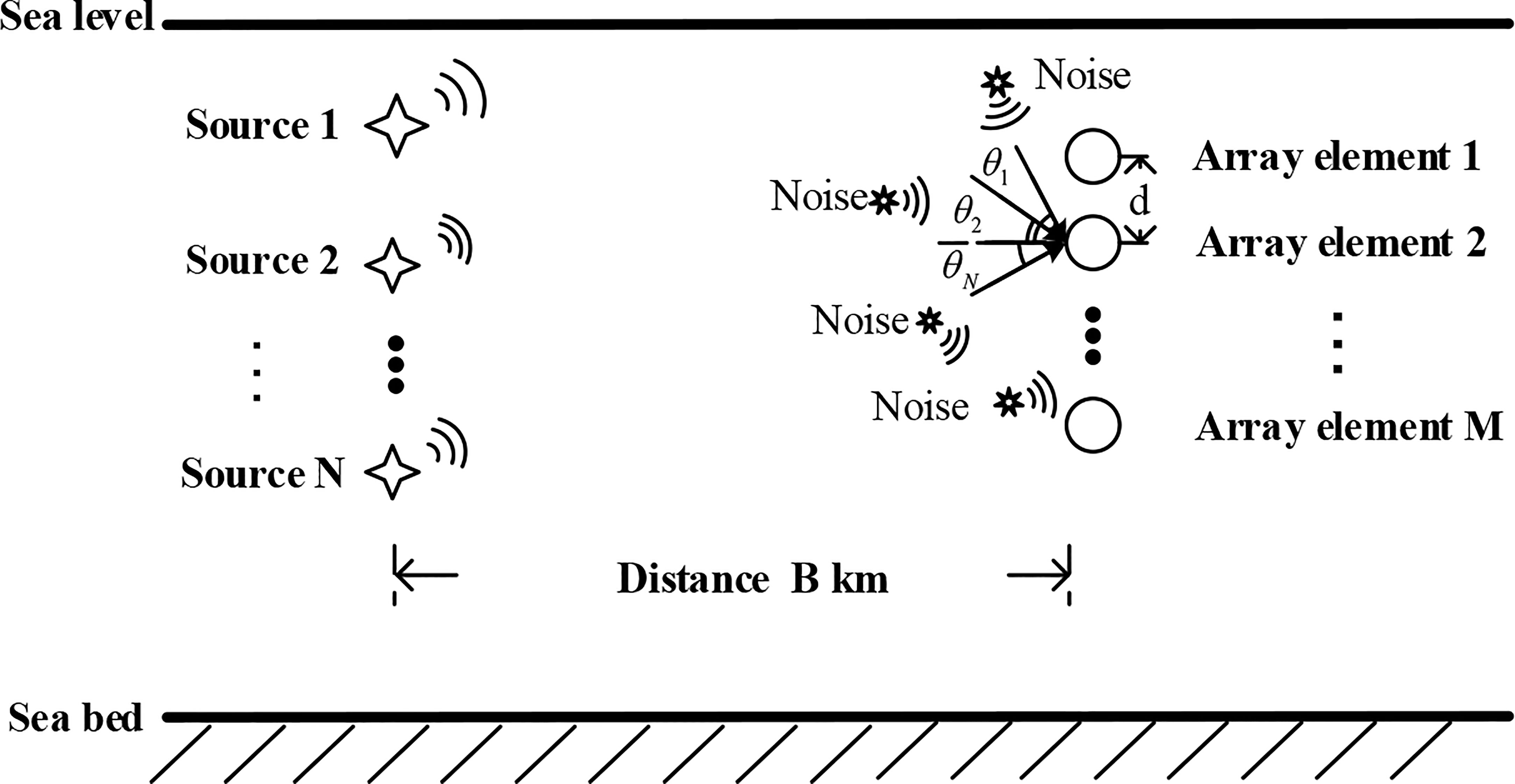
Figure 1 The DOA estimation model of an underwater acoustic array signal.
where. X(t)=[x1(t),x2(t),⋯,xM(t)]T,t=1,2,...,L ; L is the number of snapshots; Z(t)=[z1(t),z2(t),⋯,zN(t)]T represents the transmission signal of N sources at time t ; A(θ)=[a(θ1),a(θ2),⋯,a(θN)] is an M×N dimensional array manifold matrix; a(θk)=[1,e−j2πfτk,⋯,e−j2πf(M−1)τk]T is the steering vector; τk=dsinθk/c, k=1,2,⋯,N ; N(t) is the ambient noise received by the array.
The matrix form of the received signal X∈CM×L by the array is given by:
Aiming to satisfy the Nyquist sampling theorem, the traditional DOA estimation methods sample a large amount of data first, and then only a small part of the data is compressed. This approach wastes many data resources and increases hardware system complexity. To address these shortcomings, this work adopts the CS theory. First, a sparse or compressible signal is sampled at a rate much lower than the Nyquist sampling rate. Next, the projection measurement value is obtained based on the measurement matrix. Then, all information on the signal is retained, and the problem is transformed into an optimization problem. Finally, the reconstruction algorithm is used to recover the original signal. The flowchart of the CS theory is presented in Figure 2, where it can be seen that it includes sparse signal representation, measurement matrix design, and signal reconstruction algorithm.
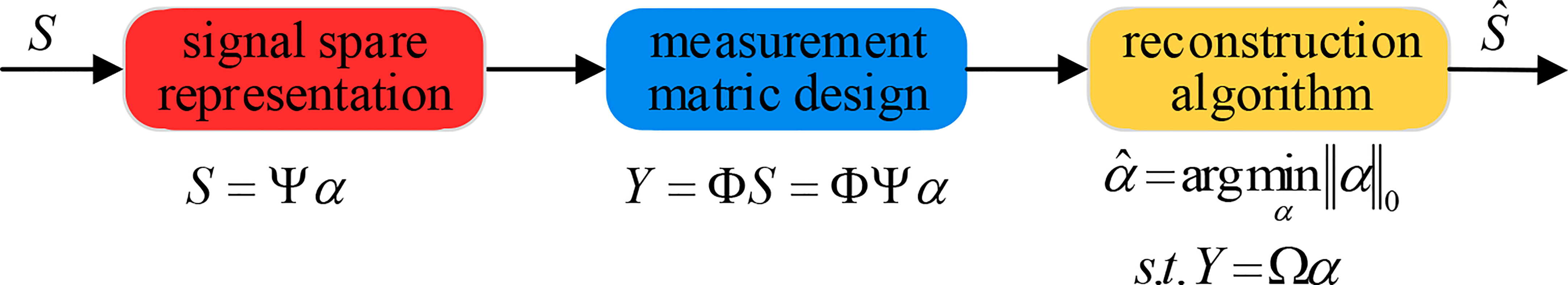
Figure 2 The flowchart of the CS theory.
Assume that there is a signal S=[s1,s2,...,sR]T in space under the action of a transform radix Ψ , which can be mathematically expressed as:
Then, the mathematical model of the DOA estimation based on the CS theory is defined by:
where Y denotes the measured value obtained through the compressed projection, Ω is the perception matrix, and Φ is the measurement matrix.
It should be noted that the CS theory can be applied only to sparse or compressible signals. However, in an underwater acoustic environment, only a few directions in the entire space have an incident source; thus, the true incoming directions of the sources are sparse for the whole space. According to Figure 1, considering the vertical array direction of the left plane of the array, the space is divided into Q(Q>>N) angles discreetly, as shown in Figure 3. The set of all possible incident directions in the space is expressed as . Therefore, the array manifold matrix , which contains the information on all angles, is used as a sparse representation matrix:
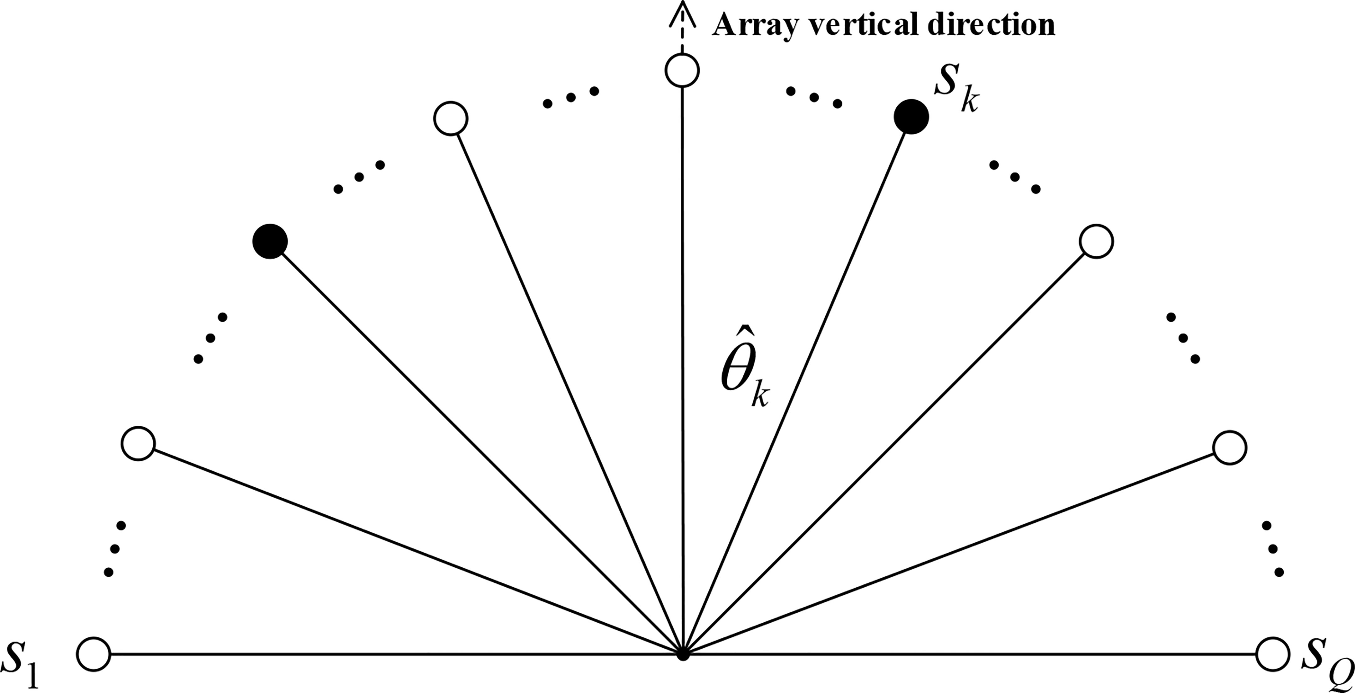
Figure 3 The schematic diagram of space division.
In matrix , each column corresponds to information about one angle, and a coefficient vector g=[g1,g2,⋯,gQ]T corresponding to is generated. The direction corresponding to the non-zero element in g indicates that there is a source incident in the angle direction; otherwise, the direction corresponding to the zero element in g indicates that there is no source incident in the angle direction. Therefore, the mathematical model of DOA estimation of an underwater acoustic signal based on the CS can be expressed as:
where X represents the received signal by the array, and is the sparse representation matrix.
Assuming that the variance of the noise received by the array in an underwater acoustic environment is δ , the coefficient vector of the reconstructed signal satisfies the following expression:
The premise of the application of DOA estimation technology based on the compressed sensing theory is to know source sparsity. In an underwater acoustic environment, a source is usually located hundreds to thousands of meters under the water surface, so it is difficult to obtain source sparsity information. This limits the promotion and application of DOA estimation technology based on the compressed sensing theory. Considering the timing characteristics of underwater acoustic signals, this paper constructs an adaptive source sparsity model based on a causal CNN. The proposed model can effectively predict source sparsity and overcome the problem that the source sparsity should be known a priori in an underwater acoustic environment.
This work uses signals received by underwater acoustic arrays as datasets. The datasets are represented as , where l denotes the sample size, is the network input, consisting of the signals received by a single element of array, , and is the classification label, which represents source sparsity, and .
The proposed adaptive source sparsity model based on a causal CNN is shown in Figure 4. The size of the convolution kernels in the first convolution layer is 1×J1 , the number of convolution kernels is W1 , and the step size is J . The first convolution layer is used to extract local features from the underwater acoustic signals. Further, in the second convolution layer, the convolution kernel size is 1×J2 , the number of convolution kernels is W2 , and the step size is one. This layer is used to enhance the correlation between local features of underwater acoustic signals. The convolution layer adopts the Leaky ReLU activation function, which is defined as follows:
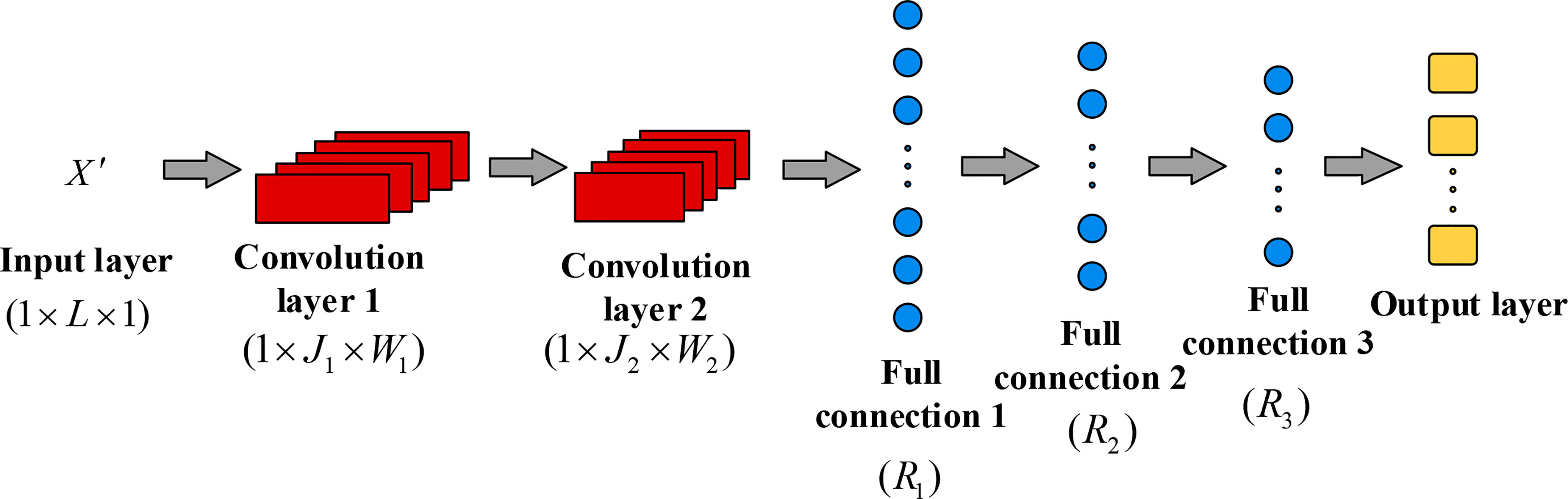
Figure 4 The proposed adaptive source sparsity model based on a causal CNN.
where x is the node output, and λ is the fixed parameter, which is in the range of (0,1) .
The output feature maps of the last convolution layer are flattened and used as input of the fully-connected layer. The third, fourth, and fifth layers are fully-connected layers and consist of R1 , R2 , and R3 neurons, respectively. The fully-connected layers are used to integrate the features. The Leaky ReLU activation function is used in the fully-connected layers. In addition, the L1 regularization is used in the fully-connected layers to avoid over-fitting, and the regularization parameter is set to β. The softmax activation function is used in the output layer, and it is given by:
where xi is the output of the i th neuron in the output layer, and C is the number of neurons in the output layer.
The output layer outputs the prediction probability of sparsity of each source, and the number of sources with the maximum prediction probability represents the prediction result of the network; then, the source sparsity G can be obtained.
The network parameters used in this study are shown in Table 1. The L1 regularization parameter of the fully-connected layer is set to 1e-5, the learning rate is set to 1e-4, and the maximum number of iterations is 500.
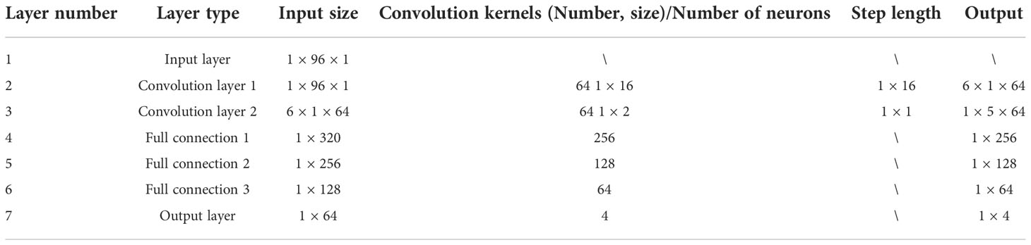
Table 1 The network parameters.
In this section, the DCMP-based DOA estimation method is presented. In this method, first, the received signal array extracts the noise subspace using the singular value decomposition (SVD) to calculate the noise power. Next, following the differentiated path screening strategy, G iterations are performed, and in each iteration, the inner product of the residual and each column in the sparse representation matrix is calculated, and atoms with large differences are selected to be stored in the differentiated candidate path set. Then, the combined path optimization strategy is adopted. Further, based on the selected differentiated candidate path set, the left and right atom approximation criteria is used to screen each group of paths, and for each group, the estimated noise power is calculated. Finally, the path group with the estimated noise power that is closest to the original noise power is selected, and the corresponding angular direction of each atom in the path group is regarded as the calculated DOA.
The two main innovations in the proposed DCMP algorithm are as follows:
(1) When screening atoms, the MMP-based DOA estimation algorithm directly screens the top η atoms with the largest current inner product; η denotes the sub-path expansion factor, which is the number of atoms screened by each inner product. It is found by simulations that the angle relationship of the previous atom with a larger inner product is very close. If the first η atoms with the largest inner product are directly taken out as a new path or a candidate set, both screening redundancy and screening time will increase. To overcome this problem, this paper proposes a differentiated path screening strategy. In each iteration, among the first η atoms with the largest inner product, only atoms whose difference exceeds γ are selected; γ denotes the differential path screening factor, which represents the atomic index difference minimum. This strategy can preliminarily determine the general angle direction, effectively reduce algorithm complexity, and improve screening efficiency while ensuring the correctness of the general angle direction.
(2) Typical termination condition in the traditional iterative greedy reconstruction algorithms is that the residual reaches the preset threshold. However, the threshold selection is greatly affected by the array element number, snapshot number, and environmental factors. Thus, it is difficult to select an appropriate threshold value. This paper proposes a combined optimization strategy, which uses the left and right atomic approximation criteria to filter the candidate path group and replace the wrongly selected atoms. Finally, this strategy takes the DOA represented by the optimal candidate path as a prediction result, which can enhance the error correction ability of the reconstruction algorithm and can also improve the estimation accuracy.
Since an underwater acoustic environment is strongly disturbed by artificial and natural noises caused by ships, industrial activities, marine organisms, and marine turbulence, the SVD of underwater acoustic signals can effectively separate signal and noise subspaces, extracts the noise subspace, and calculates the noise power for subsequent DOA estimation.
After determining the source sparsity G using the adaptive source sparsity model based the causal CNN, which is presented in Section 3, the SVD is applied to the received signal X by the array:
The noise subspace of the underwater acoustic array, which is denoted by NSV∈CM×(L−G) , is extracted as follows:
where E=[0 ones(L,L−G)] , and ones(L,L−G) represents an L×(L−G) -dimensional all one matrix.
Finally, the noise power Npower is obtained by:
The overall flowchart of the DCMP algorithm is presented in Figure 5. In this study, the DCMP algorithm is used to estimate the DOA of an underwater acoustic signal based on the received signal X by array obtained by (2); X denotes a measured value of matrix Y . The sparse representation matrix is constructed by (5), and then the source sparsity G is predicted, as explained in Section 3.2. The received signal array noise power Npower is calculated by (12). The DCMP algorithm and the noise power nearest criterion are used to select the path group , which includes indexes of G atoms from so that the estimated noise power pre_Npower of the reconstructed signal of the path group is close to Npower . The ultimate goal is to select a path combination from the reconstruction results whose noise power is the closest to the noise power of the received signal array so that (13) – (15) are satisfied.

Figure 5 The flowchart of the DCMP reconstruction algorithm.
In (13) – (15), represents the index path group corresponding to the atom filtered from ; is a column vector of (single atom); pre_NΛ represents the noise of the reconstructed signal corresponding to the path group Λ , which denotes the estimated noise; is the noise power of the reconstructed signal corresponding to path group Λ , which is the estimated noise power.The proposed DCMP reconstruction algorithm includes three main stages: initialization, differentiated path screening, and combined path screening. The three stages are presented in the following.
Assume that the initial residual is R=Y , source sparsity is G , sub path expansion factor is η (i.e., the number of atoms per inner product screening), differentiated path screening factor is γ (i.e., minimum atomic index difference), and noise power is Npower ; then, the column unitized sparse representation matrix can be expressed by:
It should be noted that this work screens only approximate angle direction in the differentiation path screening stage, which improves the screening efficiency and ensures the approximate angle direction correctness. During the differentiation path screening stage, G iterations are performed, and multiple atoms are generated in each iteration. Each atom corresponds to a different path branch, and after G iterations, multiple paths are generated, each of which is composed of G atoms and corresponds to a residual (i.e., the estimated noise). Each iteration includes ①–③, as shown below.
① Suppose that the (i−1)th iteration generates k paths denoted by and k residuals denoted by Ri−1=[r1,r2,⋯,rk] . Then, in the i th iteration, traverse k paths obtained in the (i−1)th iteration. When traversing the j th ( j=1,2,⋯,k ) path, calculate the inner product between the residual rj corresponding to the path and each atom (column) in , and sort the inner product rj values in descending order. Afterward, save the atomic index pos corresponding to the inner product values, as shown in (17). From the first η atomic indexes, select the atoms whose index difference exceeds γ and add them to the j th path Λj of the (i−1)th iteration to form a new differentiated candidate path set denoted by merge_Λ , as shown in (18) and (19).
In (17)–(19), sort() is a sort function, which is used to sort elements in descending order; index is the intermediate variable, which is used to save the index set of differentiated atoms matching rj ; , where length() is the function that returns the length of a vector, and array_merge() is a merge function, which is used to add each atom in the index to the path j in the (i−1)th iteration;
② The coefficient vector of a newly generated length(index) paths is reconstructed by the least square method. The residual value corresponding to length(index) paths is computed by:
③ Update the differentiated path set and residual of iteration as follows:
During the combined path screening stage, based on the differentiated path set , atoms on each path are further screened and replaced according to the nearest noise power principle and approximation criteria of left and right atoms for determining the optimal path group and realizing accurate DOA estimation.
The specific steps of this process are as follows:
① Suppose that a differentiated path set screened during the differentiated path screening stage contains k groups of paths, , and each path includes G atoms, . Then, the estimated noise power of each group of paths can be obtained by (14) and (15), and the noise power error is obtained by:
② The values of and its corresponding path group are sorted in ascending order, and the current optimal path group best_Λ is constructed. The minimum noise power error min_error is obtained as follows:
where inv_sort() is the ascending-order sorting function, and seq is an ascending sequence of indexes.
③ Traverse the ascending path group, and update each group of paths according to the left and right atom approximation criteria. The left and right atom approximation criteria are introduced in the following.Path group i contains G atomic indexes ( Λi=[b1,b2,⋯,bG] ), of which each corresponds to angle information. The adjacent atomic indices on both sides of G atomic indices are selected and put into con_Λ as follows:
Next, the atomic indexes in con_Λ are arranged in the way of equation (31) to obtain a new path combination new_Λ :
where j=1,2,⋯,G , and new_Λ contains a total of 3G group paths.
The estimated noise power corresponding to each group of paths in new_Λ is calculated by (14) and (15). Similarly, (13) is used to select the path group corresponding to the noise power closest to , which is denoted as an optimal path group new_Λ for this traversal, and the noise power difference new_error is saved. The iteration on this group of paths proceeds until new_error no longer decreases or the maximum number of iterations is reached, after which the path group optimization is stopped.
④ After each path iteration, it is analyzed whether new_error is less than the min_error , and if so, the min_error and best_Λ are updated; otherwise, the remaining groups of paths continue to be traversed.
Based on the combination path screening stage, the optimal path combination best_Λ is obtained. Since each atom in the path group corresponds to one DOA value, the DOA is calculated using the following expression:
where θmin is the minimum angle that can be predicted, and θinterval is the angle resolution.
The performance of the proposed algorithm was verified by simulations on a pc equipped with an Intel Core i5-9400 CPU at 2.90 GHz and an 8-GB memory. The underwater acoustic channel simulation, network dataset construction, and DCMP-based DOA estimation model were simulated in MATLAB R2018b. The adaptive source sparsity model based on causal CNN was developed using Python and Tensorflow.
In this study, the Bellhop model was used to simulate an underwater acoustic environment. The Bellhop model was selected because it is in good agreement with the actual data in the frequency range of 600 Hz–30 kHz. Therefore, this model can effectively predict channel data and simulate complex underwater acoustic environments. In addition, in this model, various environmental parameters, such as seabed surface shape, reflection and refraction losses of an acoustic wave, sound speed profile, can be set and adjusted. Further, underwater acoustic channel state parameters, such as the path number, unit impact response, and path delay, can be obtained so different underwater acoustic channels can be modeled. The signal modulation mode used in this study was BPSK; the sampling frequency was 1 kHz, and the symbol rate was 250 sps. The parameters of the marine environment are given in Table 2. The sound source and the underwater acoustic array were placed in the neritic area, and the maximum water depth was only 600 m. Environmental parameters, such as wind speed, sound speed, seawater density, and shear wave absorption coefficient, were considered. Compared with the ideal environment, such as the array and the source are located in the abyssal region and there is no wind and waves on the sea surface, the underwater acoustic environment used in this research can be considered to be relatively complex.
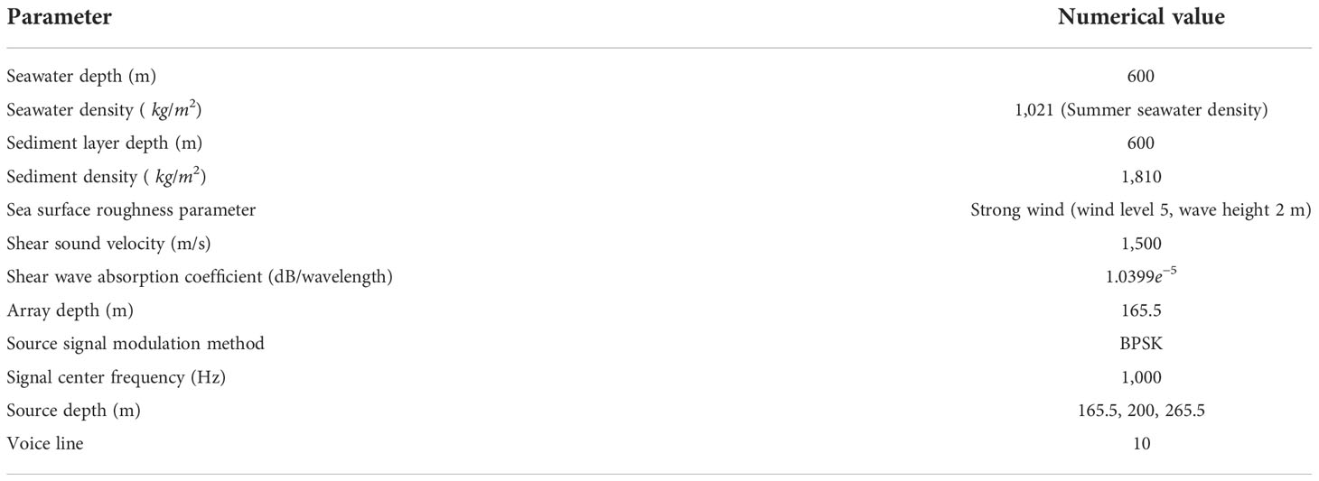
Table 2 The parameters of the marine environment.
The overall simulation flow was as follows. First, the collected underwater acoustic array signals were input into the source sparsity prediction model to obtain the source sparsity prediction results. After that, the underwater acoustic array signal and source sparsity information were input into the DOA estimation model to achieve DOA prediction.
To simulate different application scenarios, three source sparsity types, corresponding to different numbers of sources (the number of sources was one, two, or three), three commonly used array models (eight-element, 10-element, and 12-element line arrays), and seven SNR values (i.e., -5 dB, 0 dB, 5 dB, 10 dB, 15 dB, 20 dB, and 25 dB) were simulated. A total of 63 different scenarios were tested, and the element interval of the linear array was half of the signal wavelength.
To construct the network training dataset, after bellhop underwater acoustic channel modeling and array reception, the signals received by each array element were regarded as independent individual inputs into the network. For each value of sparsity, SNR, and array type 100 groups of data were collected, and the total number of input samples was 3×(8+10+12)×100×7=63,000 . The label denoted the number of source sparsity (i.e., 1, 2, or 3). The dataset was randomly divided into training and test sets according to the ratio of 7:3.
For the training dataset including three different source sparsity types, seven different SNR values, and three array types, the accuracy of the proposed model on the test set was 89.6%. To verify the impact of different scenarios on the sparsity prediction performance effectively while keeping the network structure and parameters unchanged, 1,500 groups of new data (verification set) were reconstructed to verify the network under different SNR values, array types, and source sparsity types. The verification results are shown in Table 3, where it can be seen that the prediction accuracy of the network increased with the SNR. When the SNR was higher than 10 dB, the prediction accuracy of the network reached 100%; when the SNR was -5 dB, the prediction accuracy could still reach approximately 80%. According to the results, the proposed adaptive source sparsity model based on the causal CNN could accurately predict the source sparsity under seven different SNR values and three common array models.
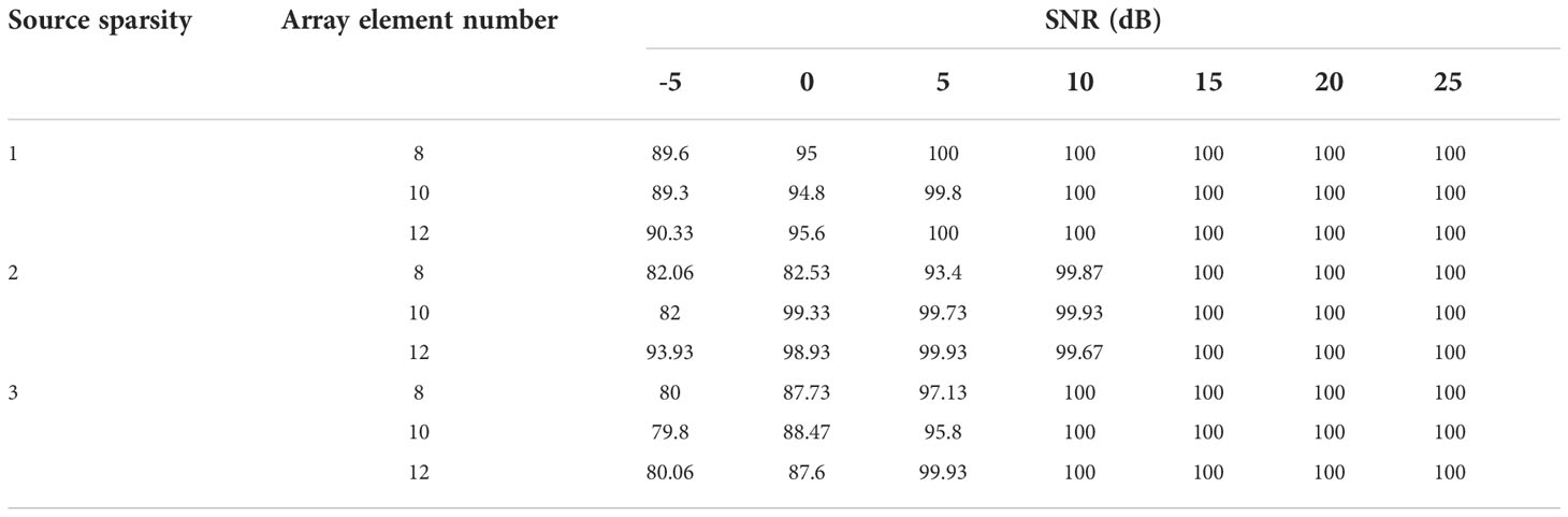
Table 3 The accuracy of the source sparsity prediction model for different SNR values, array types, and source sparsity.
To evaluate the accuracy and efficiency of the proposed reconstruction algorithm, 1,500 Monte Carlo simulations were performed under different SNR values, array types, and source sparsity types. The DOA estimation followed the source sparsity prediction in Section 5.2. The same batch of underwater acoustic array received signals was used as in Section 5.2. The performance of the proposed DCMP algorithm was compared with the performances of the orthogonal matching pursuit (OMP) algorithm and MMP algorithm. Thereinto, sparse representation matrix was constructed with an interval of 1∘ . The DOA estimation performance was evaluated in terms of accuracy, average estimation time, and mean absolute error (MAE), which are defined by (33)– (35), respectively. In (33), numerator indicates the number of simulations in which G predicted sources satisfy the constraint of , while the denominator denotes the number of simulations. The average prediction time (34) can measure the time complexity of the algorithm. The MAE (35) can indicate the prediction error of the algorithm.
In (33)–(35), θpre denotes the prediction angle; θ is the real angle; Q is the number of Monte Carlo simulations; when θpre is the same as θ , the prediction result is correct.
Considering the influence of differentiated path screening factor γ on the algorithm performance, 1,500 simulations were performed for different γ values, and the results are shown in Table 4. The simulation results indicated that the prediction accuracy of the proposed DCMP algorithm decreased with the value of γ .This was because the value of γ determined the minimum interval of atoms screened in an iteration. If the interval was too large, it led to the error that effective atoms would be misclassified into similar atoms. The average estimation time of the algorithm decreased with the value of γ, which demonstrated that the number of atoms screened in each iteration decreased, so the number of paths composed of atoms would also decrease, as well as the time loss. At the same time, the MAE increased slightly with the value of γ . Namely, when γ=10 , the accuracy of the proposed algorithm was high, and the time loss and the MAE were relatively low. Therefore, In the subsequent simulations, the value of γ was set to 10.
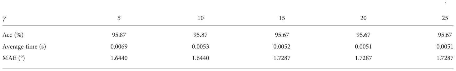
Table 4 The DCMP algorithm performance under different values of γ for two sources, the SNR of 20 dB, a 12-element array, 96 snapshots, and η=5.
The results of the accuracy, average time, and MAE of different reconstruction algorithms obtained under different source sparsity values are presented in Figure 6. As shown in Figure 6A, the prediction accuracy of all algorithms was affected by the source sparsity. When there was only one source, the prediction accuracy of the algorithms was nearly 99%; for two sources, the accuracies of MMP and OMP algorithms were less than 85%, while the accuracy of the proposed DCMP algorithm remained above 95%. The prediction accuracy results for three sources were relatively different among the algorithms. The prediction accuracy of the DCMP algorithm was still about 88%, while the accuracies of the MMP and OMP algorithms decreased to approximately 70%. With the change in source sparsity, when η=5 , the accuracy of the MMP algorithm decreased from 99% to approximately 36%; the accuracy of the OMP algorithm also fluctuated about 30%; the accuracy of the DCMP algorithm dropped from 99% to nearly 88%. Thus, the accuracy of the DCMP algorithm had little fluctuations with the change in source sparsity. As presented in (Figure 6B), the average time of the OMP algorithm fluctuated the least with an increase in source sparsity among all algorithms. The average times of the DCMP and MMP algorithms increased with the source sparsity. When η=5 , the average computation time of the DCMP algorithm was slightly longer than that of the MMP algorithm. This was due to the addition of the combined path screening stage in the DCMP algorithm. Although the DCMP algorithm had longer computation time slightly, it achieved significant accuracy improvements compared to the other algorithms. When η=10 , the average computation time of the MMP algorithm increased significantly, and it was significantly longer than that of the DCMP algorithm. Thus, adding the candidate paths increased the computation time of the MMP algorithm. On the contrary, the DCMP algorithm adopted the differentiated path screening strategy and could reduce the redundancy of candidate paths and time complexity of the algorithm effectively. Particularly, when the source sparsity was three, the average prediction time of the MMP algorithm was more than twice that of the DCMP algorithm. Further, as shown in (Figure 6C), the MAE of all reconstruction algorithms increased with the source sparsity. In the case of one source, the MAE values of the DCMP and OMP algorithms were roughly the same; meanwhile, the MAE of the MMP algorithm was slightly higher than those of the DCMP and MMP algorithms. In the multi-source scenarios (two or three sources), the MAE of the OMP algorithm was larger than 10°. However, the MAE of the DCMP algorithm was lower than 5°, and the MAE of the MMP algorithm was lower than 10°. With the increase in the η value, the MAE of the DCMP algorithm almost stayed unchanged. In the multi-source scenarios, the MAE of the MMP algorithm was slightly higher, by about 1°, than that at η=10 . Therefore, the DCMP algorithm had better estimation performance when the number of sources was greater than two.
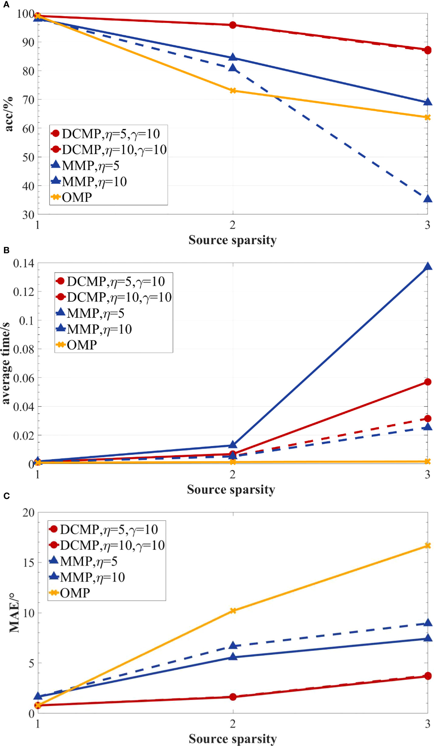
Figure 6 The performances of the DCMP, MMP, and OMP algorithms for different source sparsity under the SNR of 20 dB, a 12-element array, and 96 snapshots. (A) DOA prediction accuracy; (B) average estimation time; (C) MAE.
The results of the accuracy, average time, and MAE of the three reconstruction algorithms under different SNR values are presented in Figures 7–9. As presented in Figures 7A, 8A, and 9A, the prediction accuracy of the reconstruction algorithms increased with the SNR values. For one source and SNR of -5 dB, the prediction accuracy of the DCMP and OMP algorithms was approximately 85%. However, the accuracy of the MMP algorithm could reach only about 60%. For multiple sources (two or three sources) and seven different SNR values, the prediction accuracy of the DCMP algorithm was higher than those of the MMP and OMP algorithms. With the increase in the η values, the prediction accuracies of the DCMP and MMP algorithms also increased. In addition, compared to the DCMP algorithm, the effect of η on the MMP algorithm was more obvious. This could be because the MMP algorithm expanded η sub paths in each iteration, and adding η meant increasing the candidate paths in each iteration, which significantly improved the prediction accuracy. In the DCMP algorithm, although when η improved, only the path whose difference exceeds γ in η paths were selected, which also indicated that the angle information in each round of iteration was similar to that of the first few atoms with the largest inner product of residual R . Therefore, the gain effect of η on the DCMP algorithm was not obvious. As presented in Figures 7B, 8B, and 9B, the average computation time of each reconstruction algorithm decreased slightly with the SNR values. The average computation time of the OMP algorithm was the lowest among all algorithms. As shown in Figures 7C, 8C, and 9C, as the SNR values increased, the MAE values of all reconstruction algorithms decreased. When there was only one signal source, the MAE values of the DCMP and OMP algorithms were almost the same. But the MAE values of the DCMP algorithm was much lower than that of the MMP algorithm by 0.6°–7°. When there were two or three signal sources, the MAE of the DCMP algorithm was 0.05°–14° lower than those of the OMP and MMP algorithms. Thus, the DCMP algorithm had higher prediction accuracy than the MMP and OMP algorithm under all seven different SNR values. The average time of the DCMP algorithm was higher than that of the OMP algorithm but lower than that of the MMP algorithm. In addition, the DCMP algorithm had a lower MAE than the other two algorithms.
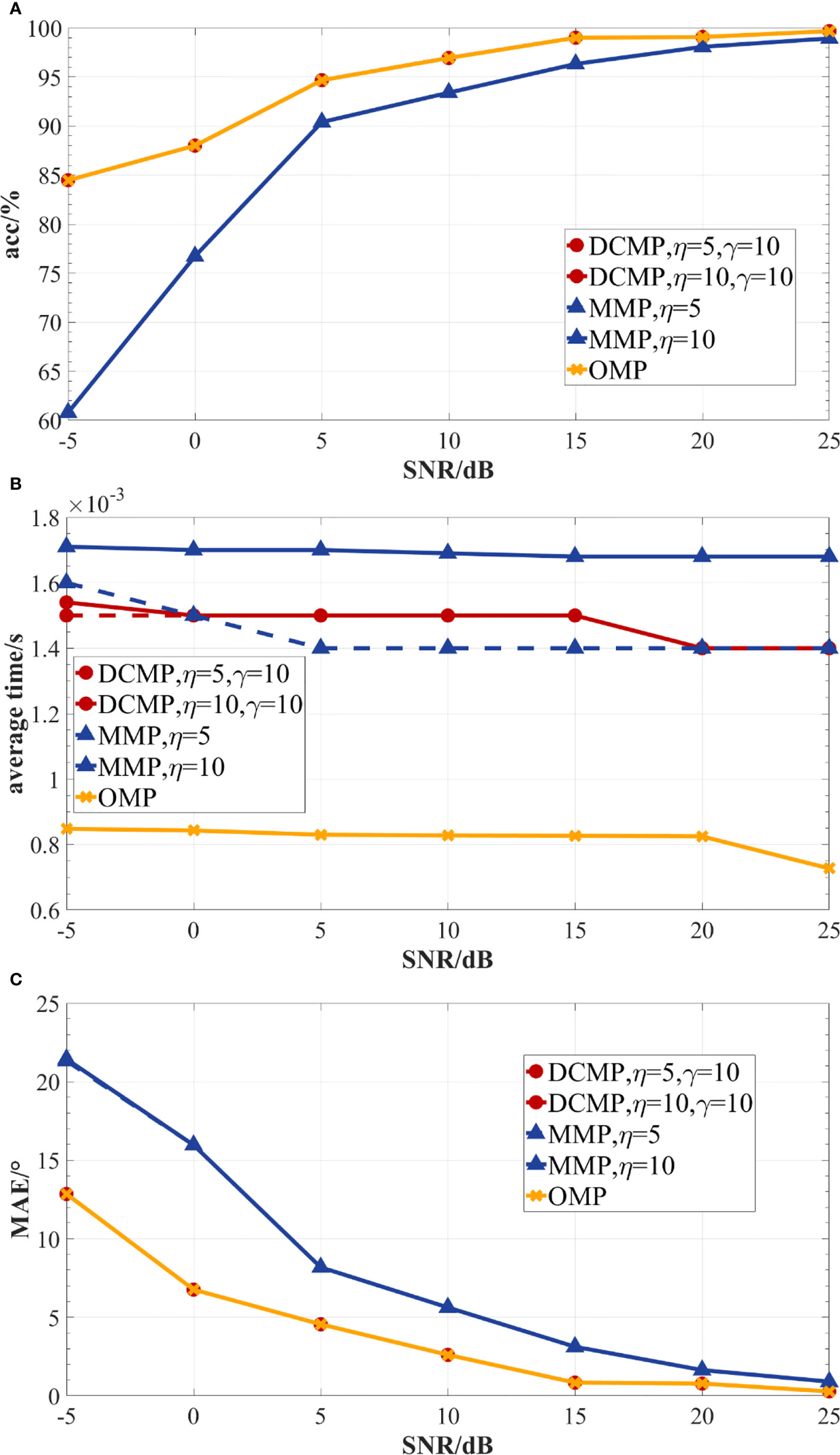
Figure 7 The performances of the DCMP, MMP, and OMP algorithms under different SNR values for one source, a 12-element array, and 96 snapshots. (A) DOA prediction accuracy; (B) average estimation time; (C) MAE.
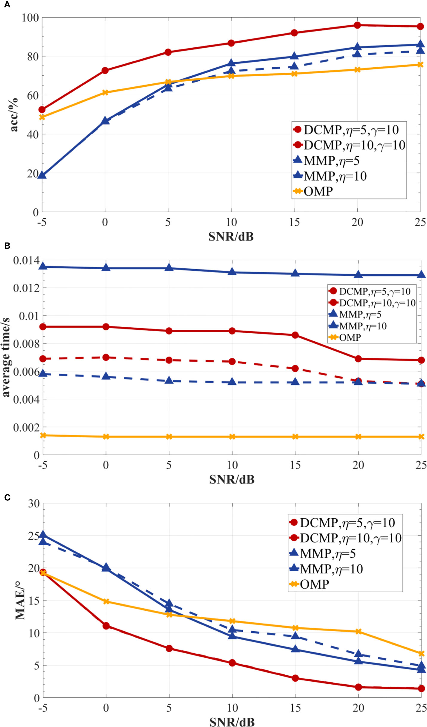
Figure 8 The performances of the DCMP, MMP, and OMP algorithms under different SNR values for two sources, a 12-element array, and 96 snapshots. (A) DOA prediction accuracy; (B) average estimation time; (C) MAE.
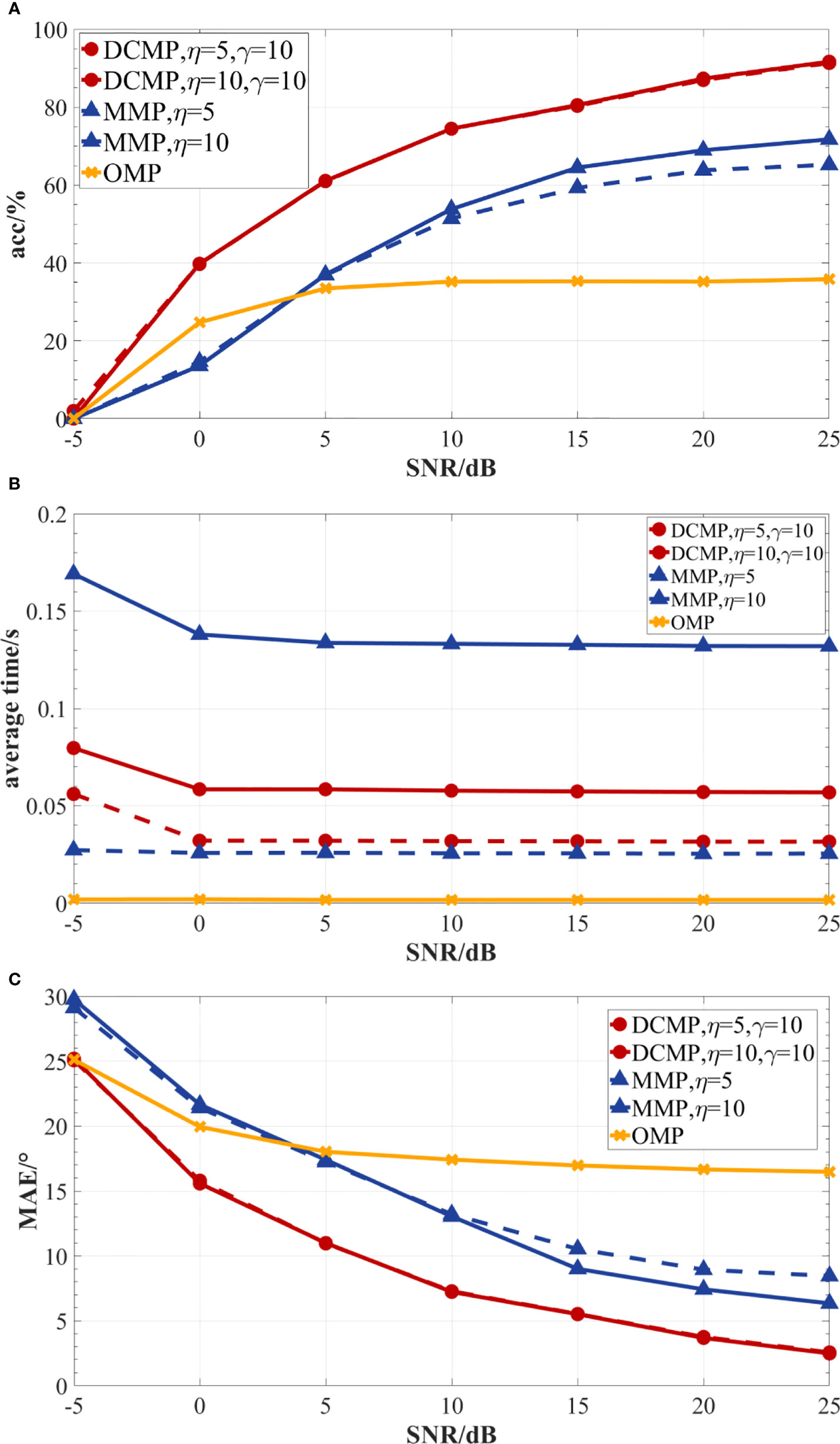
Figure 9 The performances of the DCMP, MMP, and OMP algorithms under different SNR values for three sources, a 12-element array, and 96 snapshots. (A) DOA prediction accuracy; (B) average estimation time; (C) MAE.
The accuracy, average time, and MAE results of the DCMP, MMP, and OMP algorithms obtained for different types of arrays under the conditions of a 20-dB SNR, two sources, and 96 snapshots are presented in Figure 10. As shown in Figure 10A, the accuracy of all reconstruction algorithms increased with the number of array elements. At the SNR of 20 dB, two sources, and 96 snapshots, the prediction accuracy of the DCMP algorithm could reach more than 90% under different array types. However, the highest prediction accuracy of the MMP algorithm was only 82%, while that of the OMP algorithm was even lower, only 72%. As presented in Figure 10B, the average time of all reconstruction algorithms fluctuated slightly with the number of array elements. As shown in Figure 10C, the MAE results of all three reconstruction algorithms decreased with the number of elements in the array. For different array types, the MAE value of the DCMP algorithm was much lower than those of the OMP and MMP algorithms. In summary, the DCMP algorithm showed good performance under different array types.
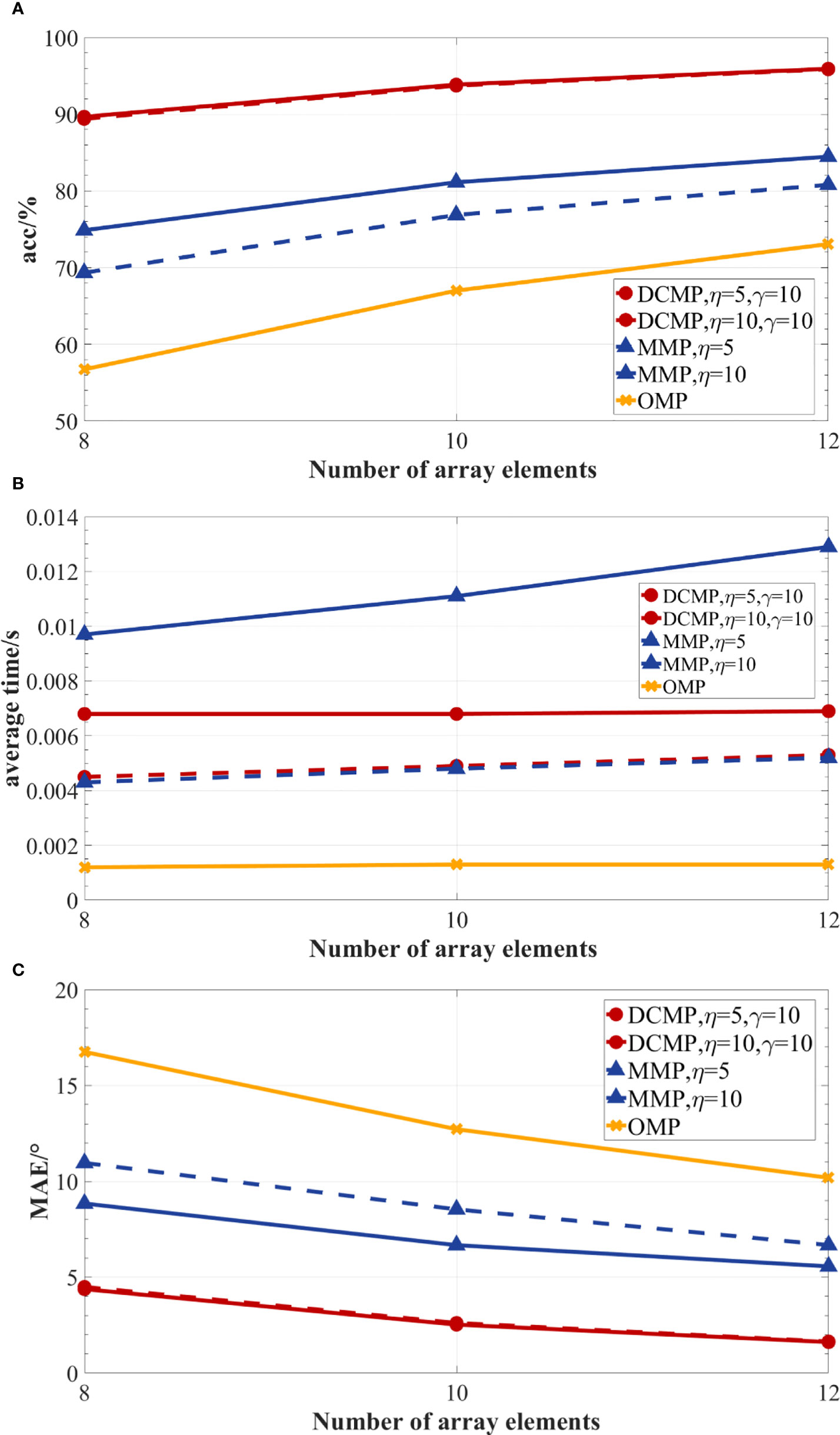
Figure 10 The performances of the DCMP, MMP, and OMP algorithms for different array types under the SNR of 20 dB, two sources, and 96 snapshots. (A) DOA prediction accuracy; (B) average estimation time; (C) MAE.
The results of the accuracy, average time, and MAE of the DCMP, MMP, and OMP algorithms based on different numbers of snapshots under the conditions of a 20-dB SNR, 2 sources, and a 12-element array are presented in Figure 11. In the simulations, the sampling points corresponding to 1, 3, 6, 12, and 22 times code elements were selected as the number of snapshots for performing the comparison. As presented in Figure 11A, the prediction accuracies of the reconstruction algorithms increased with the number of snapshots. The prediction accuracy of the proposed DCMP algorithm could still reach more than 90% at a low number of snapshots (the number of snapshots was 16), while that of the MMP algorithm can reach up to about 82%, and that of the OMP algorithm was only about 72%. As presented in Figure 11B, the average computation time of the algorithm increased with the number of snapshots. The average time of the OMP algorithm was the lowest among all algorithms, and it was less than 0.002 s. The average time of the DCMP algorithm was less than 0.01 s. However, the average time of the MMP algorithm increased significantly with the number of snapshots. When the number of snapshots was 352, the average time of the MMP algorithm was more than 0.05s. As shown in Figure 11C, the MAE of all reconstruction algorithms decreased with the number of snapshots, and the MAE of the DCMP algorithm was 2°–9° lower than those of the OMP and MMP algorithms. Therefore, the DCMP algorithm could achieve good prediction performance under a different number of snapshots while maintaining a short prediction time.
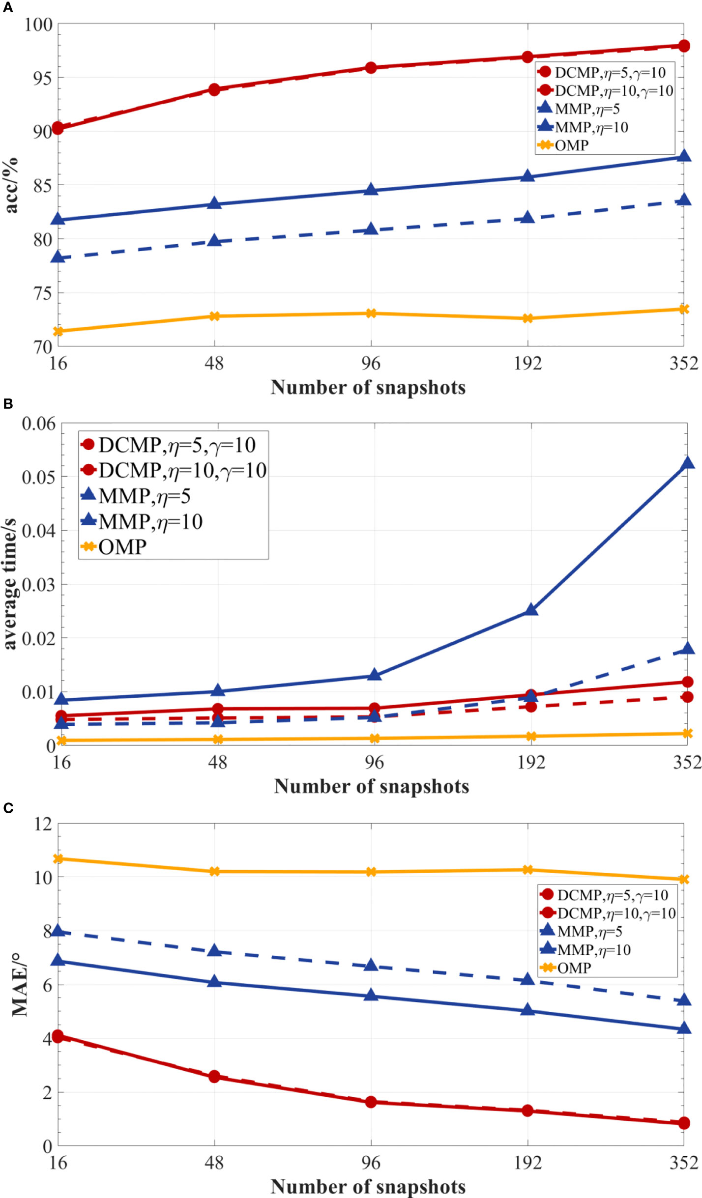
Figure 11 The performances of the DCMP, MMP, and OMP algorithms for a different number of snapshots under the SNR of 20 dB, two sources, and a 12-element array. (A) DOA prediction accuracy; (B) average estimation time; (C) MAE.
In this work, a high-precision underwater acoustic signal DOA estimation method based on sparsity adaptation is proposed. In the first part of the proposed method, an adaptive source sparsity model based on a causal CNN is used to predict source sparsity. The proposed method is verified by simulations. The simulation results show that the prediction accuracy of the proposed model can reach 100% when the SNR is higher than 10dB. In addition, the proposed model can reach a prediction accuracy of more than 80% when the SNR is less than zero, which indicates its good performance in adaptive source sparsity prediction. In the second part, a DCMP algorithm is employed. Simulation results obtained under seven different SNR values show that compared to the other reconstruction algorithms, the DCMP algorithm can improve accuracy by 9.99%–19.94%. In addition, the proposed algorithm can improve accuracy by 18.4% in a multi-source scenario, so it can be applied to multi-source application scenarios with different array types and fewer snapshots.
However, there is a certain difference in the average time between the proposed algorithm and the OMP algorithm, and MAE needs to be further reduced. In future work, more tests could be conducted to improve the performance of the proposed algorithm. Furthermore, the two-dimensional DOA estimation problem could be studied using the three-dimensional Bellhop modeling.
The raw data supporting the conclusions of this article will be made available by the authors, without undue reservation.
LJ, idea of the method. LJ, XY, and TQ, design of the study. LJ, data collection. LJ, XY, and JW, data processing and analysis. LJ, TQ, and JW, graphical abstract preparation. All authors contributed to the article and approved the submitted version.
This work was supported by the National Natural Science Foundation of China (NSFC) (Nos. U1806201, 62171246, 62101298) and the Natural Science Foundation of Shandong (ZR2021MF130, ZR2021ZD12).
The authors declare that the research was conducted in the absence of any commercial or financial relationships that could be construed as a potential conflict of interest.
All claims expressed in this article are solely those of the authors and do not necessarily represent those of their affiliated organizations, or those of the publisher, the editors and the reviewers. Any product that may be evaluated in this article, or claim that may be made by its manufacturer, is not guaranteed or endorsed by the publisher.
Ahmed A. M., Thanthrige U. M., Gamal A. E., Sezgin A. (2021). Deep learning for DOA estimation in MIMO radar systems via emulation of large antenna arrays. IEEE Commun. Letters. 25 (5), 1559–1563. doi: 10.1109/LCOMM.2021.3053114
Candes E., Romberg J. K., Tao T. (2006). Robust uncertainty principles: Exact signal reconstruction from highly incomplete frequency information. IEEE Trans. Inf. Theory. 52 (2), 489–509. doi: 10.1109/TIT.2005.862083
Candes E., Tao T. (2005). Decoding by linear programming. IEEE Trans. Inf. Theory 51 (12), 4203–4215. doi: 10.1109/TIT.2005.858979
Cui W., Guo S. X., Tao J. W. (2021). Reconstruction for sparse signal based on bidirectional sparsity adaptive and weak selection of atoms matching pursuit. Circuits Syst. Signal Processing. 40 (10), 4850–4876. doi: 10.1007/S00034-021-01695-9
Cui W., Shen Q., Liu W., Wu S. L. (2019). Low complexity DOA estimation for wideband off-grid sources based on re-focused compressive sensing with dynamic dictionary. IEEE J. Selected Topics Signal Processing. 13 (5), 918–930. doi: 10.1109/JSTSP.2019.2932973
Do T., Gan L., Nam N., Tran T. (2008). “Sparsity adaptive matching pursuit algorithm for practical compressed sensing,” in Proceedings of the 42nd Asilomar Conference on Signals, Systems and Computers (Pacific Grove, CA), 581–587. doi: 10.1109/ACSSC.2008.5074472
Fu Q., Jing B., He P. (2019). Blind DOA estimation in a reverberant environment based on hybrid initialized multichannel deep 2-d convolutional NMF with feedback mechanism. IEEE Access. 7, 179679–179689. doi: 10.1109/ACCESS.2019.2958955
Fu Y. S., Liu S. S., Ren C. H. (2016). Adaptive step-size matching pursuit algorithm for practical sparse reconstruction. Circuits Syst. Signal Processing. 36 (6), 2275–2291. doi: 10.1007/s00034-016-0393-5
He Y. C., Wang F., Wang S. Y., Cao S. Y., Chen B. D. (2019). Maximum correntropy adaption filtering approach for robust compressive sensing reconstruction. Inf. Sci. 480, 381–402. doi: 10.1016/j.ins.2018.12.039
Jia T. Y., Wang H. Y., Shen X. H. (2020). A study of compressed sensing single-snapshot DOA estimation based on the RIPless theory. Telecommunication Systems. 74 (4), 531–537. doi: 10.1007/s11235-020-00676-8
Kase Y., Nishimura T., Ohgane T., Ogawa Y., Sato T., Kishiyama Y. (2022). Accuracy improvement in DOA estimation with deep learning. IEICE Trans. Commun. E105B (5), 588–599. doi: 10.1587/transcom.2021ebt0001
Kim B. S., Jin Y., Lee J., Kim S. (2020). Low-complexity MUSIC-based direction-of-arrival detection algorithm for frequency-modulated continuous-wave vital radar. Sensors. 20 (15), 4295. doi: 10.3390/s20154295
Li N., Yin X. H., Guo H. Y., Zong S. L., Fu W. (2020). Variable step-size matching pursuit based on oblique projection for compressed sensing. IET Image Processing. 14 (4), 766–773. doi: 10.1049/iet-ipr.2019.0916
Lu X. M., Su Y. W., Wu Q., Wei Y. H. (2022). An improved algorithm of segmented orthogonal matching pursuit based on wireless sensor networks. Int. J. Distributed Sensor Networks. 18 (3), 15501329221077165. doi: 10.1177/15501329221077165
Roy R., Kailath T. (1986). ESPRIT-estimation of signal parameters via rotational invariance techniques. IEEE Trans. Acoustics Speech Signal Processing. 37 (7), 984–995. doi: 10.1109/29.32276
Schmidt R., Schmidt R. O. (1986). Multiple emitter location and signal parameter estimation. IEEE Transaction Antennas Propagation. 36 (3), 276–280. doi: 10.1109/TAP.1986.1143830
Vallet P., Mestre X., Loubation P. (2015). Performance analysis of an improved MUSIC DOA estimator. IEEE Trans. Signal Processing. 63 (23), 6407–6422. doi: 10.1109/TSP.2015.2465302
Varanasi V., Gupta H., Hegde R. M. (2020). A deep learning framework for robust DOA estimation using spherical harmonic decomposition. IEEE/ACM Trans. Audio Speech Lang. Processing. 28, 1248–1259. doi: 10.1109/TASLP.2020.2984852
Wang H. T., Wang J., Jiang J. Z., Liao K. F. (2022). Target detection and DOA estimation for passive bistatic radar in the presence of residual interference. Remote Sens. 14 (4), 1044. doi: 10.3390/rs14041044
Wei Y. B., Lu Z. Z., Yuan G. B., Fang Z., Huang Y. (2017). Sparsity adaptive matching pursuit detection algorithm based on compressed sensing for radar signals. Sensors. 17 (5), 1120–1133. doi: 10.3390/s17051120
Yan H. C., Chen T., Wang P., Zhang L. M., Cheng R., Bai Y. P. (2021). A direction-of-arrival estimation algorithm based on compressed sensing and density-based spatial clustering and its application in signal processing of MEMS vector hydrophone. Sensors. 21 (6), 2191–2215. doi: 10.3390/s21062191
Keywords: the direction of arrival estimation, underwater acoustic array signal processing, compressed sensing, reconstruction algorithm, deep learning
Citation: Jiao L, Yang X, Quan T and Wang J (2022) High-precision DOA estimation for underwater acoustic signals based on sparsity adaptation. Front. Mar. Sci. 9:1022494. doi: 10.3389/fmars.2022.1022494
Received: 18 August 2022; Accepted: 03 November 2022;
Published: 23 November 2022.
Edited by:
Kun Yang, Zhejiang Ocean University, ChinaReviewed by:
Chen Zhao, Wuhan University, ChinaCopyright © 2022 Jiao, Yang, Quan and Wang. This is an open-access article distributed under the terms of the Creative Commons Attribution License (CC BY). The use, distribution or reproduction in other forums is permitted, provided the original author(s) and the copyright owner(s) are credited and that the original publication in this journal is cited, in accordance with accepted academic practice. No use, distribution or reproduction is permitted which does not comply with these terms.
*Correspondence: Xinghai Yang, eWFuZ3hoQHF1c3QuZWR1LmNu
Disclaimer: All claims expressed in this article are solely those of the authors and do not necessarily represent those of their affiliated organizations, or those of the publisher, the editors and the reviewers. Any product that may be evaluated in this article or claim that may be made by its manufacturer is not guaranteed or endorsed by the publisher.
Research integrity at Frontiers
Learn more about the work of our research integrity team to safeguard the quality of each article we publish.