Determining the drift characteristics of open lifeboats based on large-scale drift experiments

Lifeboat is one of the most important life-saving equipment for escaping at sea when a ship is abandoned in an extreme emergency. An accurate drift model can help rescuers find the drift position of lifeboat in the shortest time, thus improving the efficiency of marine search and rescue (SAR) at sea and ensuring the safety of wrecked people. The purpose of this paper is to investigate the drift characteristics and to develop an accurate drift prediction model for the open lifeboat. First, large-scale drift experiments were conducted to analyze the drift characteristics with three 6.5-meter-long real-size open lifeboats in the South China Sea. Next, three drift prediction models of the lifeboats were developed using the least squares method based on the drift experimental data. Finally, the drift prediction models of the lifeboats were compared and evaluated using the Lagrangian method and Monte Carlo technique, respectively. Results indicate that the probability of positive crosswind leeway (CWL) of the open lifeboat is 47.5%. The jibing frequency is 6% per hour, and the maximum leeway divergence angle is 45°. These drift characteristics are very important for the prediction of the open lifeboat drift trajectory. The comparison results of three drift models show that the improved drift model is more accurate than the other two drift models for predicting drift trajectories of the open lifeboat, which can be directly applied to maritime search and rescue operations in the South China Sea.

Highlights

● A series of maritime drift experiments on three open lifeboats were performed in the South China Sea.

● The drift characteristics of the open lifeboats in the South China Sea were determined.

● The improved drift prediction model was established for the open lifeboats in the South China Sea.

Introduction

Every year, thousands of people lose their lives at sea as a result of ship accidents around the world. (Serra et al., 2020). As one of the most important life-saving equipment for ships, lifeboats play a vital role when ships are in distress, especially a ship needs to be abandoned in an extreme emergency. An accurate drift model can help rescuers find the drift position of the lifeboat in the shortest time, thus improving the efficiency of marine search and rescue (SAR) at sea. The free drift of the lifeboat at sea is driven by wind, currents and waves (Huang et al., 2011; Brushett et al., 2016; Cucco et al., 2016; Yulmetov et al., 2016; Ličer et al., 2020; Ivić et al., 2020). Predicting the trajectories of wrecked objects in the marine environment, like lifeboats, requires information about the characteristics of the objects (Liu and Weisberg, 2011; Röhrs et al., 2012). The drift characteristics vary from one type of maritime drifting objects to another, so their drift coefficients, which are usually obtained by using linear regression analysis based on huge amounts of data from field experiments.

The research on the drift characteristics of wrecked objects at sea has attracted people’s attention since World War II, and the research methods have become more efficient with technological advances and the development of experimental instruments. The methods can be divided into two categories: direct method and indirect method. The direct method uses a current meter (also GPS tracking) directly connected to the drifting object to measure the drifting speed of the object (Allen and Plourde, 1999; Allen, 2005; Breivik et al., 2011). The indirect method measures the drift speed of the object indirectly due to the limitation of the measuring instrument (Breivik et al., 2013). The study of the drift characteristics of wrecked targets also provides technical support for the establishment of maritime SAR platforms. At present, more mature search and rescue platforms include the Search and Rescue Planning Program (CANSARP) of Canada, the Modèle Océanique de Transport d’Hydrocarbures (MOTHY) system of French (Daniel et al., 2003), the Search and Rescue Mapping and Analysis Program (SARMAP) of U.S. Applied Science Associates and the Search and Rescue Optimal Planning System (SAROPS) of U.S. Coast Guard (Kratzke et al., 2010).

With the development of modern technology, maritime search and rescue work has made great progress, especially the use of emergency position indicating radio beacon (EPIRB), emergency Locator Transmitter (ELT) and personal Locator Beacon (PLB), is playing an increasingly important role in maritime search and rescue work. The International Maritime Organization (IMO) has also promoted and encouraged ships at sea to be equipped with EPIRBs, and sailors to be equipped with PLBs when working at sea, in case of maritime accidents, which can greatly improve the efficiency of search and rescue and save more lives. However, on the other hand, EPIRB, ELT and PLB may fail in harsh and complex marine environments. Therefore, it is necessary to develop efficient and accurate drift prediction techniques for shipwrecked targets at sea.

The core of predicting the trajectory of wrecked objects in maritime search and rescue is to establishing drift model. Allen and Plourde (1999; 2005) proposed a leeway model, which defines leeway as the drift motion of an object due to surface wind (10 m height) and surface currents (0.3~1.0 m depth) and quantifies the drift velocity based on statistical data from a large number of sea drift experiments on SAR targets. This model has been extensively used for a variety of marine search and rescue targets, including persons-in-the-water, fishing boats, life rafts, containers and others (Allen et al., 2010; Breivik et al., 2011; Breivik et al., 2012; Brushett et al., 2014; Brushett et al., 2017; Xu et al., 2017; Zhou et al., 2020; Yang et al., 2021). Zhang et al. (2017) established a dynamic drift model, which holds that when the velocity of a drifting object is stable, the forces of current and wind acting on the object reach a balance. This model does not consider the effect of wave force on the drifting object. There are significant differences between the leeway model and the dynamic drift model. In the leeway model, the leeway is decomposed into the downwind component and crosswind component, and the crosswind component has left or right deviation along the downwind, which can accurately express the influence of the wind on the drifting target. However, the dynamic drift model cannot express the influence of the wind on the drifting target well, especially the phenomenon of the wind direction changing (Zhu et al., 2019). The leeway model ignores the dissipation of the current force on the object, and the current coefficient is approximately regarded as 1.0. The dynamic model gives the relationship between the drift velocity, wind velocity and current velocity, and can well express the dissipation of the current force on the drifting target.

With the rapid increasement of fishing, transportation and offshore construction activities in the South China Sea, maritime safety accidents occur frequently. For example, on July 2, 2022, the offshore wind power construction ship “Fujing 001” sank off the coast of Yangjiang in the South China Sea. Thirty sailors abandoned the engineering ship when it broke up. Although equipped with escape equipment, 25 sailors lost their lives due to the inability to accurately predict the target drift position. Therefore, accurate drift prediction model is very important for maritime search and rescue work. This paper proposed an improved drift prediction model on the basis of the dynamic model and the leeway model for the open lifeboats in the South China Sea. Free drift experiments on three 6.5-meter-long real-size open lifeboats were conducted in the South China Sea to collect drift data and meteorological data. The leeway drift model, the dynamic drift model and the improved drift model for the open lifeboats were then established. Finally, Lagrangian particle tracking method and Monte Carlo technique were adopted to evaluate the accuracy of three drift models of the open lifeboat. The research results of this paper can be directly applied to maritime search and rescue work in the South China Sea.

Drift models and evaluation methods

Dynamic drift model

The dynamic drift model ignores the effect of acceleration of the object at sea and simplifies the wave forces. It assumes that the drift motions of objects at sea are only affected by currents and winds. The above part of the object is affected by the wind forces and the underwater part is affected by the current forces. The forces are dependent on the relative velocity between the object and current or wind. According to the law of motion, when the object is drifting at steady speed, the two forces should be opposite and added up to zero. The following is an expression for the dynamic drift model (Zhang et al., 2017):

$\begin{array}{ll}\begin{array}{l}\frac{1}{2}{\rho }_{air}{C}_{air}{S}_{air}|{\overrightarrow{V}}_{wind}-{\overrightarrow{V}}_O|({\overrightarrow{V}}_{wind}-{\overrightarrow{V}}_O)+\\ \frac{1}{2}{\rho }_{water}{C}_{water}{S}_{water}|{\overrightarrow{V}}_{current}-{\overrightarrow{V}}_O|({\overrightarrow{V}}_{current}-{\overrightarrow{V}}_O)=0\end{array}& (1)\end{array}$

where ${\overrightarrow{V}}_O$ denotes the drift velocity, ${\overrightarrow{V}}_{wind}$ denotes the wind speed (10 m reference height), and ${\overrightarrow{V}}_{current}$ denotes the current speed. C stands for the drag coefficient, S stands for the cross-sectional area, ρ stands for the density, and the subscripts represent air and water. The model can be simplified as:

$\begin{array}{ll}\begin{array}{c}{\overrightarrow{V}}_O=\frac{1}{1+\alpha }{\overrightarrow{V}}_{current}+\frac{\alpha }{1+\alpha }{\overrightarrow{V}}_{wind}\end{array}& (2)\end{array}$

where $\alpha =\sqrt{{\rho }_{air}{C}_{air}{S}_{air}/{\rho }_{water}{C}_{water}{S}_{water}}$, and setting λ=1/(1+α) , the model can be further simplified as:

$\begin{array}{ll}\begin{array}{c}{\overrightarrow{V}}_O=\lambda {\overrightarrow{V}}_{current}+(1-\lambda ){\overrightarrow{V}}_{wind}\end{array}& (3)\end{array}$

Leeway drift model

Allen and Plourde (1999; 2005) proposed and further developed the leeway model based on large quantities of drift data from sea experiments. This model was adopted in the international aeronautical and maritime SAR manual to calculate the drift of a shipwrecked target. According to the model, different shapes of objects have different drift rules and characteristics, and for the majority of drifting objects (lengths are less than wavelengths), the wave forces can be disregarded (Breivik and Allen, 2008). A drift target’s velocity can be written as:

$\begin{array}{ll}\begin{array}{c}{\overrightarrow{V}}_O={\overrightarrow{V}}_{F-current}+\overrightarrow{L}\end{array}& (4)\end{array}$

where ${\overrightarrow{V}}_O$ is the drifting object’s velocity, ${\overrightarrow{V}}_{F-current}$ is the current-generated velocity (typically regarded as being equivalent to the current speed of near-surface), and $\overrightarrow{L}$ is the wind-induced drift velocity. It can be seen that the drift speed of a drifting object is the sum of the action of currents and winds.

The fluctuations of the leeway angle at low wind velocity could not be accurately expressed by early leeway model. Allen (2005) divided the Leeway into two components: the crosswind leeway component (CWL) and the downwind leeway component (DWL) (Figure 1). People usually regard that the probability of positive CWL (right of the downwind) and negative CWL (left of the downwind) for the crosswind leeway component is equal. Nevertheless, the variation in the direction of the crosswind leeway component is extremely complex. The concept of “jibing” is proposed by Allen to quantify the phenomenon of the leeway direction of a drifting object transform from left to right (or from right to left) along the downwind.

FIGURE 1

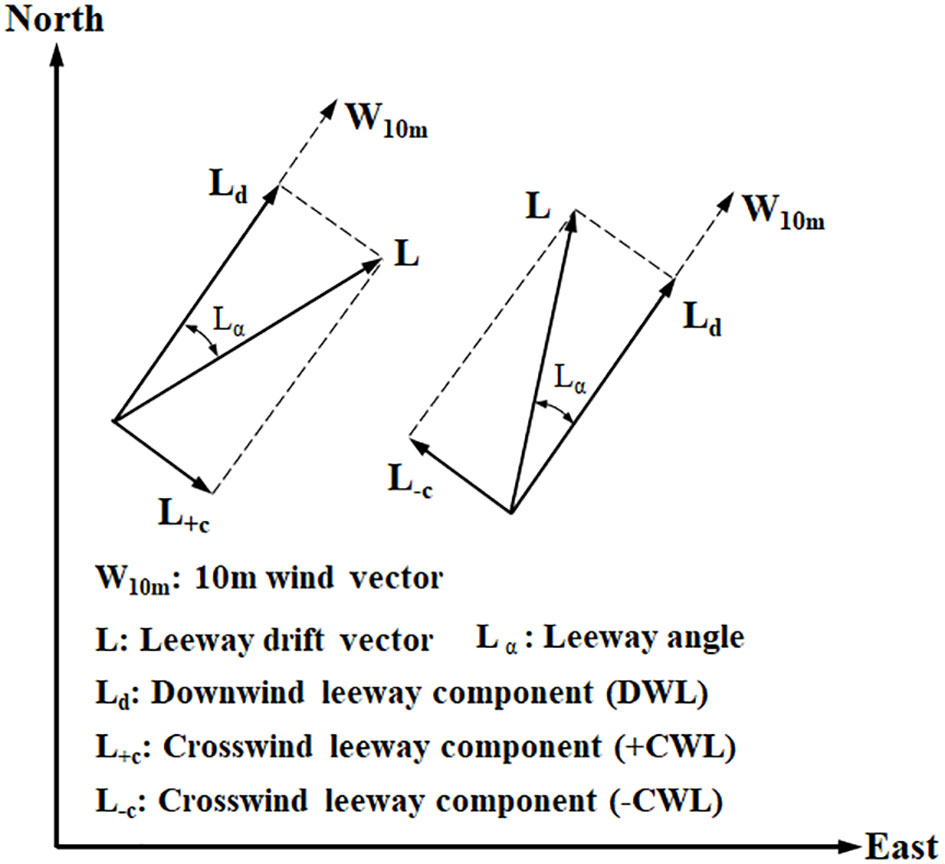
Figure 1 The relationship between the leeway drift vector, the downwind leeway component and the crosswind leeway component.

When using the leeway model to predict the drift of an object at sea, it is necessary to input 9 leeway coefficients and some marine environmental Information. The nine coefficients are the slope, intercept and standard deviation of the three regression equations, which are obtained by linear regression method based on large amounts of drift experimental data. Thus, the Leeway model is expressed mathematically as follows:

$\begin{array}{ll}\begin{array}{c}\{\begin{array}{c}\overrightarrow{L}={\overrightarrow{L}}_d+{\overrightarrow{L}}_c\\ L_d=a_d{V}_{wind}+b_d+{ϵ}_d(DWL)\\ L_{+c}=a_{+c}{V}_{wind}+b_{+c}+{ϵ}_{+c}(+CWL)\\ L_{-c}=a_{-c}{V}_{wind}+b_{-c}+{ϵ}_{-c}(-CWL)\end{array}\end{array}& (5)\end{array}$

where L_d stands for the downwind leeway, which has a linear relationship with wind speed V_wind (10 m reference height), L_+c stands for the positive crosswind leeway component, L_-c stands for the negative crosswind leeway component, a_d , a_+c , a_−c are the slope of the three linear equations, b_d , b_+c , b_−c are the offset of the three linear equations, and ϵ_d , ϵ_+c , ϵ_−c are the error term of the three linear equations,

Improved drift model

The leeway model ignores the dissipation of the current drag force acting on the marine target by the current and takes the current velocity as the current-induced drift velocity. But the drift velocity component caused by the current is not exactly equal to the current velocity, which results in a certain error when predicting drift velocity with the leeway model. The dynamic drift model uses linear regression to obtain the contribution coefficients of the wind and the current to the drift velocity, but its prediction of drift direction is not accurate enough. This paper proposes an improved drift model. The leeway coefficient is determined using the leeway model method, while the current-induced drift coefficient is determined using the dynamic drift model method. Thus, the prediction accuracy of drift velocity can be improved. The drifting object’s motion velocity can be expressed as follows:

$\begin{array}{ll}\begin{array}{c}{\overrightarrow{V}}_O=k{\overrightarrow{V}}_{current}+\overrightarrow{L}\end{array}& (6)\end{array}$

where ${\overrightarrow{V}}_O$ stands for the drift velocity, ${\overrightarrow{V}}_{current}$ stands for the current velocity, $\overrightarrow{L}$ stands for the object’s leeway, k and ${\overrightarrow{V}}_{current}$ stand for the current-induced drift coefficient and the current velocity, respectively. The leeway and wind velocity have a similar relationship both in the downwind direction and the crosswind direction as Eq. (5).

Lagrangian particle tracking method and Monte Carlo method

In order to compare and verify the effectiveness of the three models for the drift of open lifeboats at sea, the Lagrangian particle tracking method was used to simulate the drift trajectory of open lifeboats. Following is the leeway model’s particle tracking motion equation:

$\begin{array}{ll}\begin{array}{c}x(t)=x(t_0)+{\displaystyle {\int }_{t_0}^t{\overrightarrow{V}}_O(t^{\prime })d{t}^{\prime }=x(t_0)}+{\displaystyle {\int }_{t_0}^t\left[\lambda {\overrightarrow{V}}_{current}(t^{\prime })+(1-\lambda ){\overrightarrow{V}}_{wind}(t^{\prime })\right]d{t}^{\prime }}\end{array}\#(7)& (7)\end{array}$

and for the dynamic drift model it is:

$\begin{array}{ll}\begin{array}{c}x(t)=x(t_0)+{\displaystyle {\int }_{t_0}^t{\overrightarrow{V}}_O(t^{\prime })d{t}^{\prime }=x(t_0)}+{\displaystyle {\int }_{t_0}^t\left[{\overrightarrow{V}}_{F-current}(t^{\prime })+\overrightarrow{L}(t^{\prime })\right]d{t}^{\prime }}\end{array}& (8)\end{array}$

and for the improved drift model it is:

$\begin{array}{ll}\begin{array}{c}x(t)=x(t_0)+{\displaystyle {\int }_{t_0}^t{\overrightarrow{V}}_O(t^{\prime })d{t}^{\prime }=x(t_0)}+{\displaystyle {\int }_{t_0}^t\left[k{\overrightarrow{V}}_{current}(t^{\prime })+\overrightarrow{L}(t^{\prime })\right]d{t}^{\prime }}\end{array}& (9)\end{array}$

Since the calculations of the leeway model and the improved drift model take into account the probability of positive CWL (POPC), which makes the results of the Lagrangian particle tracking method potentially random. Monte Carlo method is further employed to evaluate the leeway model and the improved model to remedy this deficiency. The perturbation of marine environment and initial position are not taken into consideration because of the effects on the CWL sign change cannot directly measure in the sea experiments. The coefficients from the leeway model serve as the only perturbation in the simulations. When the Monte Carlo method is used in this paper, 1000 particles are set for simulation. Meanwhile, POPC and jibing frequency were considered to make the simulation results more accurate. In order to consider the uncertainty caused by the experimental errors, it is necessary to perturb the leeway coefficients. The disturbance formula of the jth particle is:

$\begin{array}{ll}\begin{array}{c}{a}_j=a+\frac{S_{\frac{y}{x}}{\tau }_j}{20}\end{array}& (10)\end{array}$

$\begin{array}{ll}\begin{array}{c}{b}_j=b+\frac{S_{\frac{y}{x}}{\tau }_j}{2}\end{array}& (11)\end{array}$

$\begin{array}{ll}\begin{array}{c}{\tau }_j\in N(0,1)\end{array}& (12)\end{array}$

where a_j and b_j are the j th particle’s leeway coefficients, τ_j stands for the perturbation of the j th particle’s leeway coefficient, and τ_j is a random number, which follows a normal distribution.

Drifting experiment at sea

Experiment subjects

To build the drift models for lifeboats, three 6.5 meter-long real-size open lifeboats with empty weight were used in the experiments to simulate free drift under the actual sea conditions. Three identical lifeboats were used to avoid the randomness of a single sample. The lifeboats in transportation and in the ocean are shown in Figure 2. The principal dimensions of the lifeboats are summarized in Table 1. As shown in Table 1, the open lifeboats used in the experiment are 6.5 m length, 2.15 m breadth and 0.90 m depth. They can carry up to 21 people, and have an empty weight of 1839 kg and a full load weight of 3414 kg.

FIGURE 2

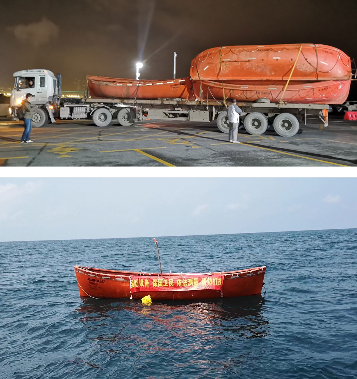
Figure 2 The open lifeboats used in the experiments.

TABLE 1

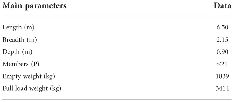
Table 1 Performance parameters of the open lifeboats.

Experimental instruments

The “Specifications for oceanographic survey-Part 2: Marine Hydrographic observation” and “Specifications for oceanographic survey-Part 3: Marine Meteorological observations” were used as guidelines for the experimental data collection. A Nortek Signature ADCP and a Nortek Aquadopp ADCP were used to collect current data in the experiment, and an AirMar 220WX weather station was used to collect wind data. Figure 3 depicts the installation of the instruments, and Table 2 lists the pertinent parameters.

FIGURE 3

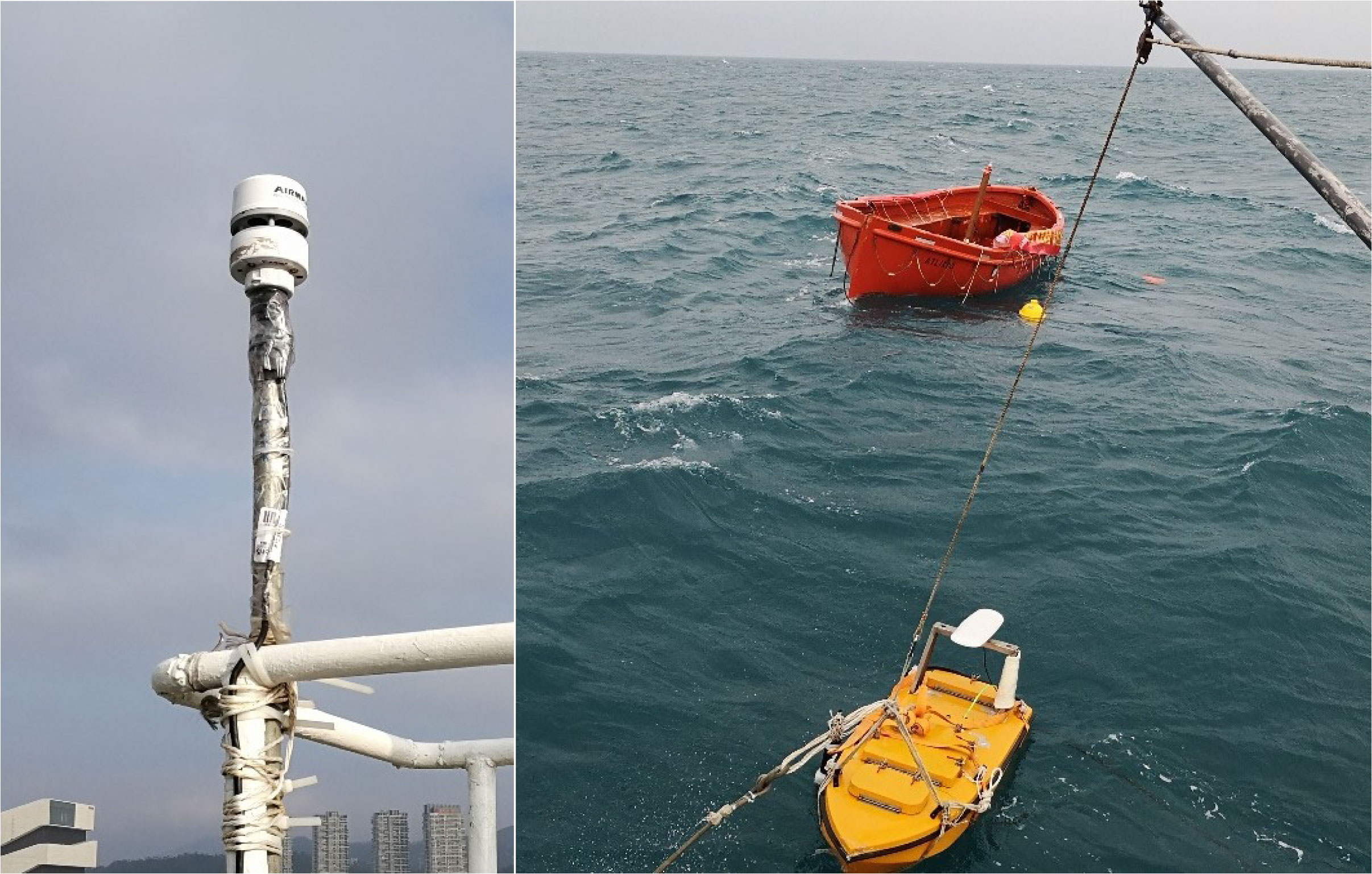
Figure 3 Installation of AirMar 220WX weather station (left), Nortek AquaDopp ADCP, Nortek Signature ADCP and GPS receiver (right).

TABLE 2

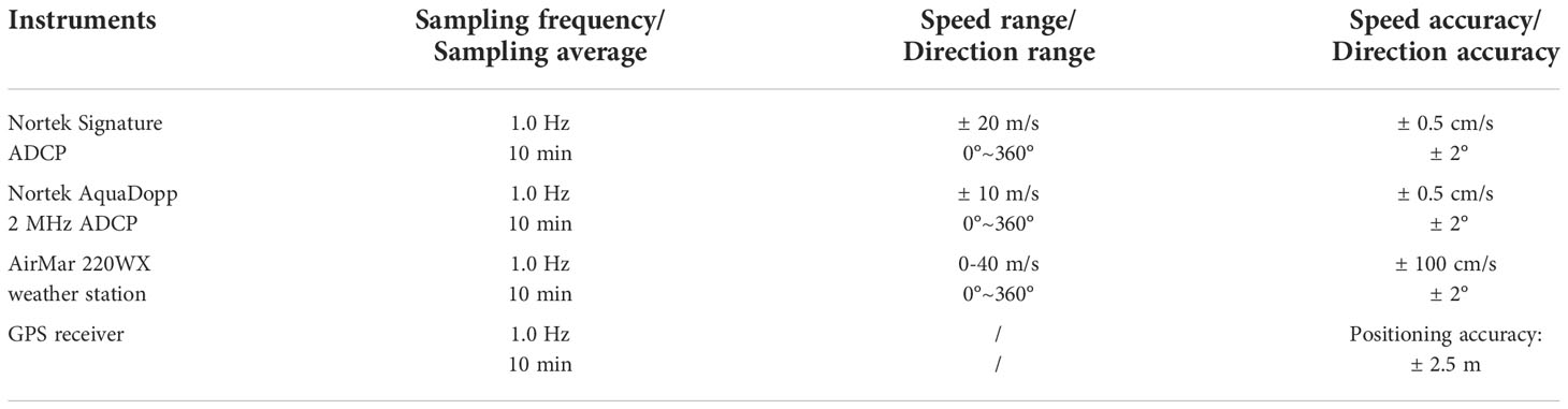
Table 2 Performance parameters of the experimental instruments.

To measure the surface current speed close the lifeboat, the Nortek Signature ADCP with 500 KHz and the Aquadopp ADCP with 2 MHz were fixed to a custom ship buoy and the ship buoy was allowed to float freely around the lifeboat to obtain the current speed. The sampling frequency of ADCP was set at 1 HZ. The current data acquired every 10 minutes was then compiled into a group. A high-precision positioning module is built into the ADCP, allowing it to record its own moving velocity in real-time and automatically correct the actual current speed. One set of wind speed data was collected every minute by the weather station, which was mounted on the survey boat about 9 meters above the water"s surface. The observed wind speed was then converted to the wind speed at the standard 10 meters reference height according to the wind speed conversion formula.

$\begin{array}{ll}{U}_{10}=\frac{\ln \left(\frac{10}{Z_0}\right)}{\ln \left(\frac{Z}{Z_0}\right)}{U}_Z& (13)\end{array}$

Where U₁₀ is the wind speed at 10 m above the sea level, Z is the height of the observed wind speed, U_z is the observed wind speed. When the wind speed is greater than 7 m/s, Z_{0 =} 0.022, and when the wind speed is not greater than 7 m/s, Z_{0 =} 0.023. The built-in positioning system was programmed to send back the position data of the lifeboat every 10 minutes. Figure 3 depicts how the instruments were installed.

Experimental procedure

From April 4 to 10, 2019, we conducted lifeboat at-sea drift tracking observation experiments in the China South Sea. Three important drift track samples were obtained during the roughly 68 hours of tracking observations that were completed. We obtained 360 samples by breaking these data down into 10-minute averages. The experimental area and the actual drift trajectories of the lifeboats during the experiments are shown in Figure 4. It contains trajectories of walkaround observation and trajectories that are not under walking observation (tracking only the positions). The red line indicates the trajectory of the first lifeboat drift experiment conducted on April 4, 2019, with a tracking observation time of about 24 hours. The yellow line indicates the trajectory of the second lifeboat drift experiment conducted on April 6, with a tracking observation time of about 24 hours, and the green line indicates the trajectory of the third lifeboat drift experiment conducted on April 9, with a tracking observation time of about 20 hours.

FIGURE 4

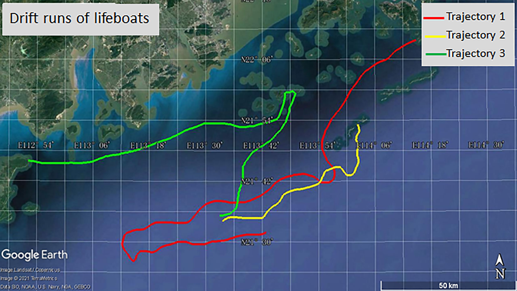
Figure 4 Drift trajectories and experimental zone.

The specific steps of the experiment are as follows.

(1) Pre-test preparations. The 500 KHz frequency ADCP and 2 MHz frequency Aquadopp ADCP were installed on the custom buoy, and the weather station was installed on the survey vessel at a height of about 9 m above the water surface. The experimenter debugged the equipment again to ensure the normal operation of the equipment.

(2) The survey vessel departed from a coastal port with lifeboats as well as observation equipment and proceeded to a predetermined location. GPS was used to record the trajectory. When the survey vessel arrived at the predetermined station, an anchor is needed to stabilize the ship, the experimenter recorded the initial position information of the survey vessel (GPS) and measured the water depth. Then the lifeboat and a small wave observation buoy were released and connected by ropes. Installing the GPS positioning system in the lifeboat and set the GPS to send back the position information of the lifeboat every ten minutes. Sandbags were evenly placed inside the lifeboat as the ballast. Custom buoys were hoisted and placed, which were connected to the survey vessel by ropes and released 10-20 m away from the survey vessel to shut out the impact of the vessel’s own turbulence.

(3) The survey vessel weighed anchor and follows the lifeboat with a custom buoy to start the walk-around observation. The ADCP observed from the surface downward and stabilizes its direction with a gimbal every 0.5 m. The Aquadopp ADCP recorded the surface current velocity from 0.5-1 m at a single point with a sampling frequency of 1 HZ. The weather station collected 1 set of wind speed and wind direction data every minute. In the course of walk-around observation, the survey vessel should be located 40-50m behind the side of the lifeboats to ensure the validity of the observation data and avoid the shielding effect of the superstructure of the vessel on the lifeboats from wind and wave.

(4) After 25 hours of continuous observation, the tracking observation of lifeboats ended. The observation equipment was recovered and the survey vessel returned to shore. After the vessel arrived ashore, the experimenter immediately played back saved the data observed by ADCP, Aquadopp, weather station and GPS.

(5) In order to assess the subsequent drift models, the lifeboat continued to drift, and the GPS continuously recorded the positioning data after the end of the walk-around observation. Ground wave radar and offshore weather stations continuously monitored the sea trial area.

Results and analysis

Experiment results

The values and directions of the lifeboat drift velocity, current velocity and wind velocity during the drift experiment with time are shown in Figures 5, 6. The black line represents the drift speed of the lifeboat, the blue line represents the flow velocity, and the orange line represents the wind velocity. During the continuous drift from April 4 to 5, 2019, the wind speed was in the range of 4-10 m/s and the current speed was in the range of 0-0.4 m/s. The lifeboat drifted at 0.3-0.8 m/s, slightly greater than the current speed. The wind speed and current direction were around 270° (with a northerly direction of 0° and an easterly direction of 90°), and the lifeboat drifted in the direction between the wind direction and the current direction. In the continuous drift from April 6 to 7, the wind speed was in the range of 0-6 m/s and the current speed was in the range of 0-0.4 m/s. The lifeboat drifted at 0.2-0.6 m/s. The drift direction of the lifeboat was first around 90° and then decreased in the range of 0°-90°. During the continuous drift from April 9 to 10, the wind speed was in the range of 3-6 m/s and the current speed was in the range of 0.1-0.7 m/s. The drift speed of the lifeboat was in the range of 0.1-0.6 m/s. The drift direction of the lifeboat gradually decreased from about 90° to about 0°.

FIGURE 5

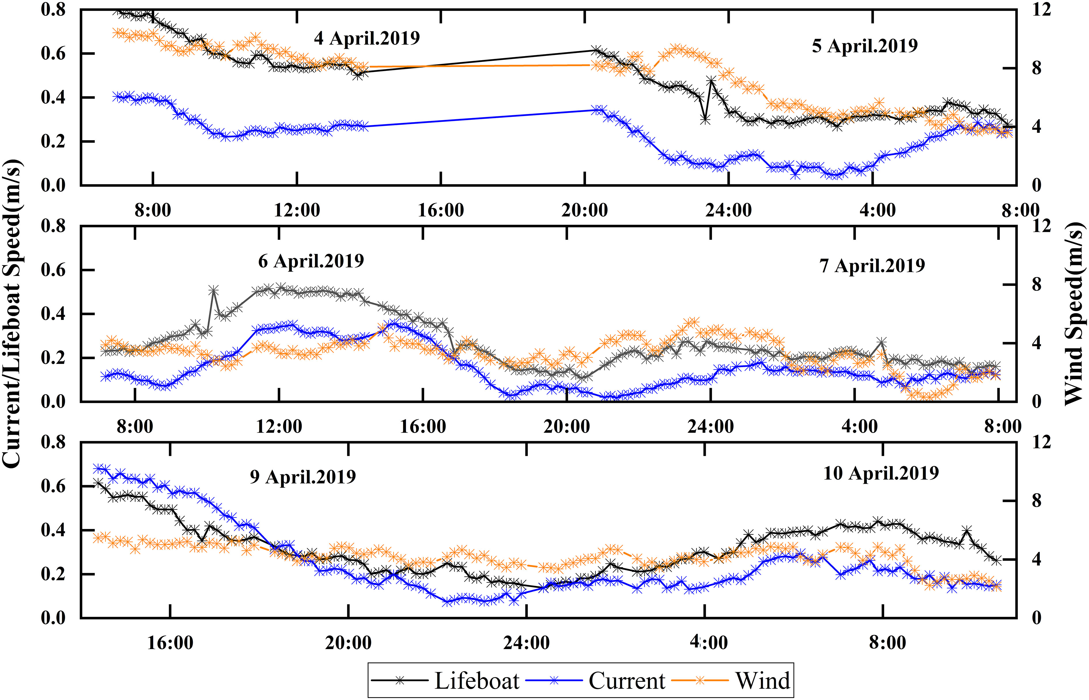
Figure 5 Values of drift speed, wind speed and current speed over time for the open lifeboat, with the black lines representing the open lifeboat, the blue lines representing the current, and the orange lines representing the wind.

FIGURE 6

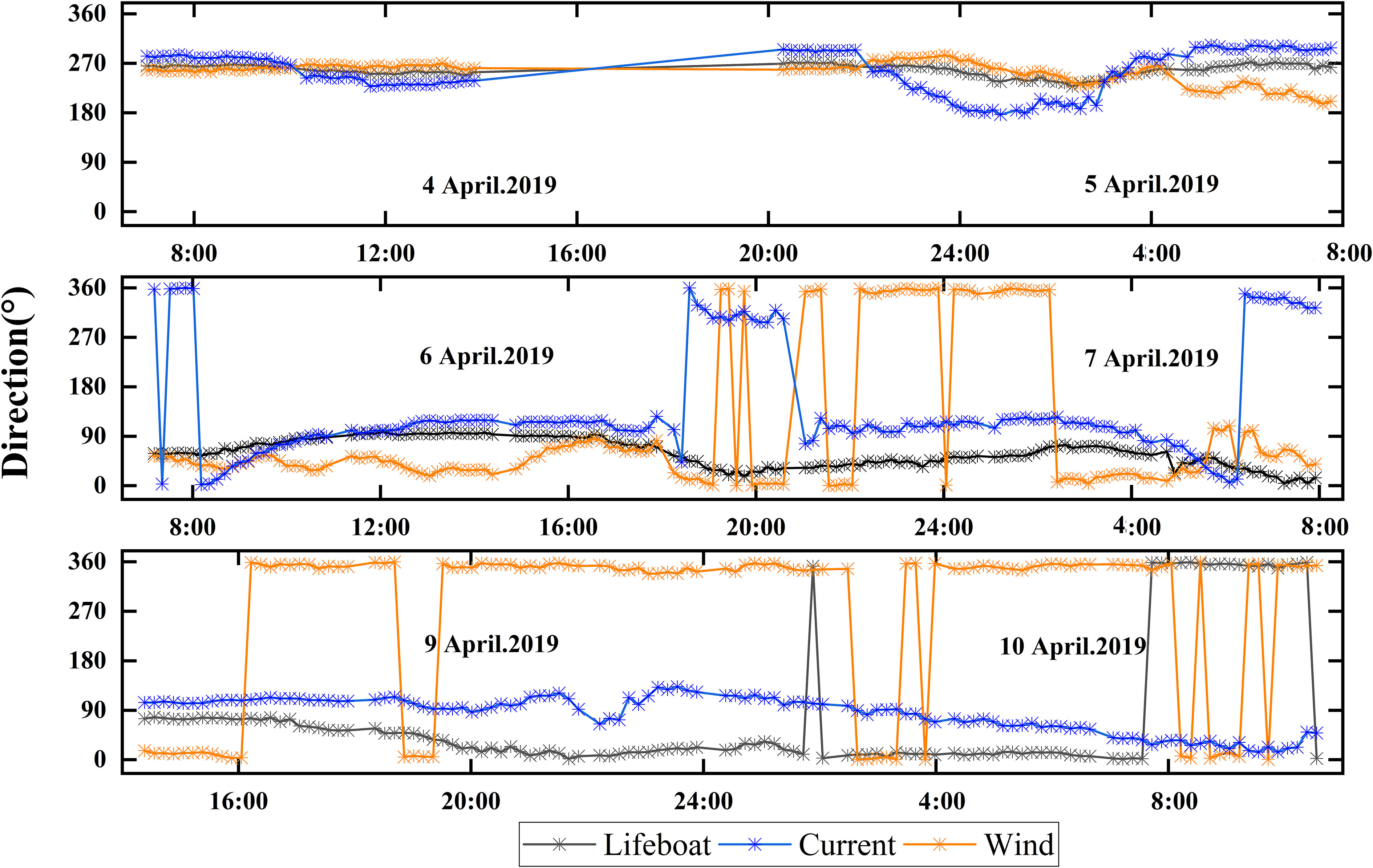
Figure 6 Directions of drift speed, wind speed and current speed over time for the open lifeboat, with the black lines representing the open lifeboat, the blue lines representing the current, and the orange lines representing the wind.

The statistical information of the number of crosswinds, jibing frequency and leeway divergence is recorded in Table 3. As can be seen, the open lifeboat’s probability of having a positive CWL is 47.5%. As an important indicator of drift characteristics, jibing frequency can be determined by the number of jibing events occurring within a period of drift. And the jibing events of the lifeboat can be described by progressive vector diagram (PVD) of downwind drift distance and the crosswind drift distance. The relationship between the downwind and the crosswind drift distance for the open lifeboat in the three drifts is shown in Figure 7. From the PVD diagram, there were four jibing events of the open lifeboat during the drift in about 68 hours. Therefore, the jibing frequency of the open lifeboat is 6%. Also, the maximum leeway divergence angle of the open lifeboat is found to be 45° from Figure 7.

TABLE 3

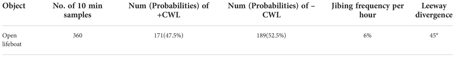
Table 3 Statistics on the quantity of crosswinds, the frequency of jibing, and the leeway divergence.

FIGURE 7

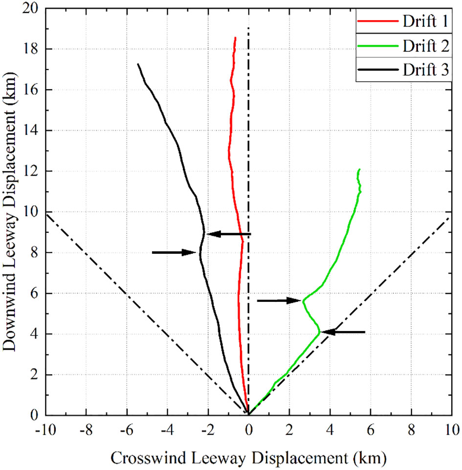
Figure 7 Leeway displacement for the open lifeboat as depicted in a progressive vector diagram (PVD) for the downwind and crosswind components. Black arrows represent jibing events.

Establishment of dynamic drift model

All of the vectors in Eq. (5) are ${\overrightarrow{V}}_O$, ${\overrightarrow{V}}_{current}$, and ${\overrightarrow{V}}_{wind}$. The wind speed, the current speed, and the drift velocity were divided into components in the X direction (east) and components in the Y direction (north) to enable linear regression via the least squares method. Figure 8 show the regression outcomes of the dynamic drift model for the open lifeboat. Table 4 shows the optimum estimations of the dynamic model’s regression coefficients Λ. The open lifeboat’s X-direction parameter Λ_X is 0.9584, and its Y-direction parameter Λ_Y is 0.9503, and its coefficient of determination R² values are 0.9433 and 0.8707, respectively. This means that the model can simulate the object’s velocity in relation to the current and wind speed well. In addition, it can be seen that the drift coefficients in the X-direction and the Y-direction have different magnitudes due to the different magnitudes of the object drift velocity, wind speed and current velocity components in the X-direction and Y-direction.

FIGURE 8

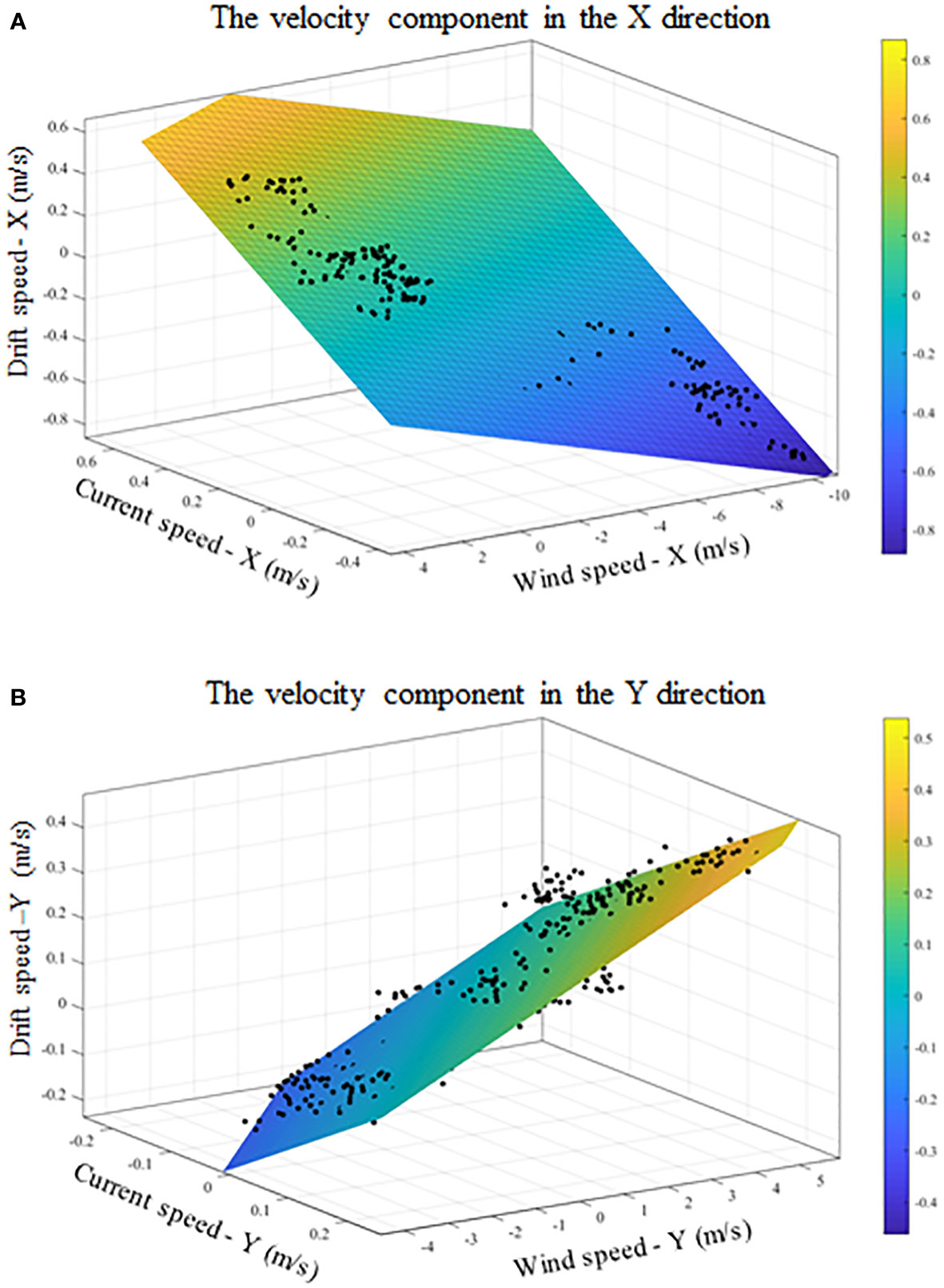
Figure 8 The relationship between the wind velocity and the current velocity and the drift velocity of the open lifeboat in the X direction (A) and the Y direction (B).

TABLE 4

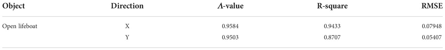
Table 4 Linear regression results of dynamic model coefficients.

According to the results of the dynamic model parameters in Table 5, the expression of the dynamic drift model of the open lifeboat can be obtained as follows:

$$\{\begin{array}{c}{\overrightarrow{V}}_{lifeboat}={\overrightarrow{V}}_{lifeboat-x}+{\overrightarrow{V}}_{lifeboat-y}\\ V_{lifeboat-x}=0.95841V_{current-x}+0.0416V_{wind-x}\\ V_{lifeboat-y}=0.9503V_{current-y}+0.0497V_{wind-y}\end{array}$$

TABLE 5

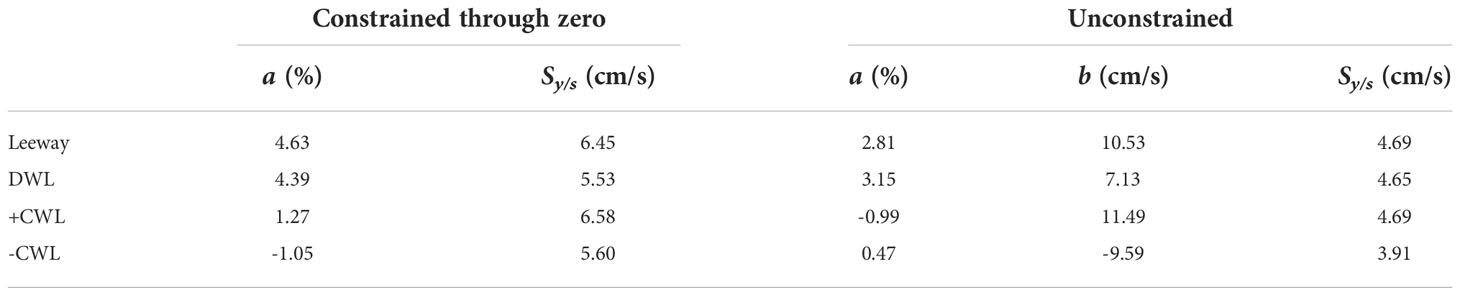
Table 5 The regression coefficients and standard errors.

Establishment of leeway drift model

The open lifeboat’s leeway drift coefficients were calculated using the method of regression analysis based on the experiment’s data for wind, current, and drift speeds. Figure 9 depicts the regression analysis results of leeway velocity, DWL, and CWL for the leeway drift model. The zero linear regression constraint is shown by the solid green line. The unrestricted linear regression is shown by the solid red line. The 95% confidence intervals for the regressions are shown by dashed lines. Table 5 displays the regression coefficients and standard errors. The regression coefficient ( a ) represents the slope of the leeway drift formula, ( b ) the intercept, and (S_y/x) the regression’s standard error.

FIGURE 9

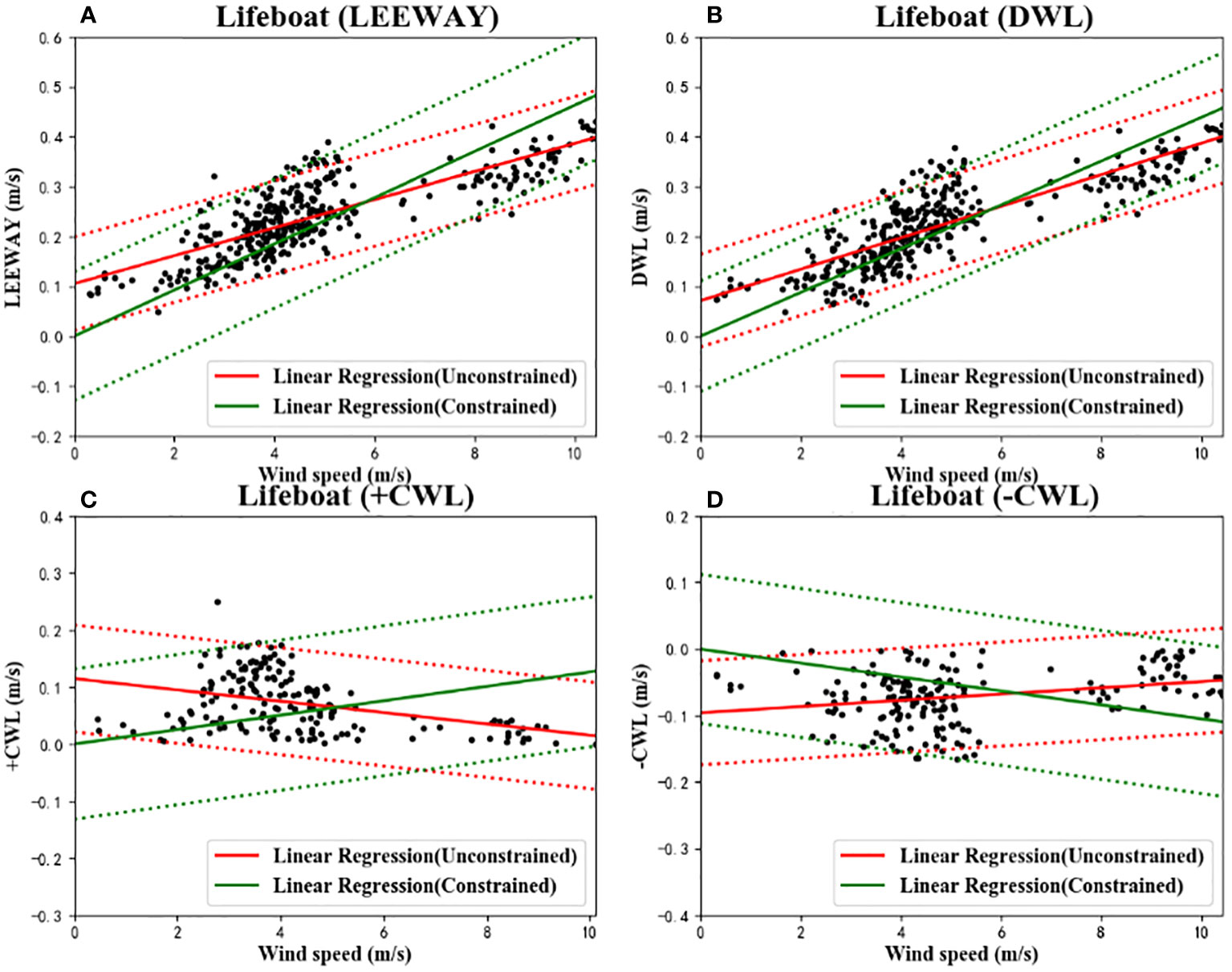
Figure 9 The linear regressions and 95% confidence level statistics of Leeway Speed (A), DWL (B), +CWL (C) and –CWL (D) with 10 m height wind speed for the leeway drift model. Unconstrained linear regression (solid) and 95% of the confidence levels (dash) are plotted in red, while constrained linear regression is plotted in green.

The coefficient of determination R² was used to assess how strong the linear relationship was between the wind velocity the leeway components and at a height of 10 m. In the constrained and unconstrained cases, the R² values of DWL for the open lifeboat are 0.60 and 0.69, respectively. The effect of the regression analysis is expressed by the R² value. The closer the R² value is to 1, the better the fit of the equation is. Typically, unconstrained R² values are higher than constrained R² values. In addition, the CWL to the left or right of the wind direction is random and varies in magnitude, resulting in a difference between +CWL and -CWL, and therefore, it needs to be separately determined. Since the magnitudes of +CWL and -CWL are different, the coefficients are also different.

The leeway drift model expression for the open lifeboat is obtained from the unconstrained leeway coefficient results in Table 4 as follows:

$$\{\begin{array}{c}{\overrightarrow{V}}_{lifeboat}={\overrightarrow{V}}_{current}+\overrightarrow{L}={\overrightarrow{V}}_{current}+{\overrightarrow{L}}_d+{\overrightarrow{L}}_c\\ L_d=3.15\%V_{wind}+7.13 cm/s;{\text{ S}}_{\frac{y}{x}}=4.65cm/s\\ L_{+c}=-0.99\%V_{wind}+11.49 cm/s;{\text{ S}}_{\frac{y}{x}}=4.69cm/s\\ L_{-c}=0.47\%V_{wind}-9.59 cm/s;{\text{ S}}_{\frac{y}{x}}=3.91cm/s\end{array}$$

Construction of improved model

Firstly, it needs to replace the coefficient λ in the dynamic model of Section 4.3 with coefficient k in formula (6), and the leeway velocity is recalculated. After that, the regression analysis method is used to calculate the new leeway coefficients for the open lifeboat based on the new leeway velocity and wind speed. Figure 10 shows the regression analysis results of leeway velocity, DWL, and CWL for the improved model.

FIGURE 10

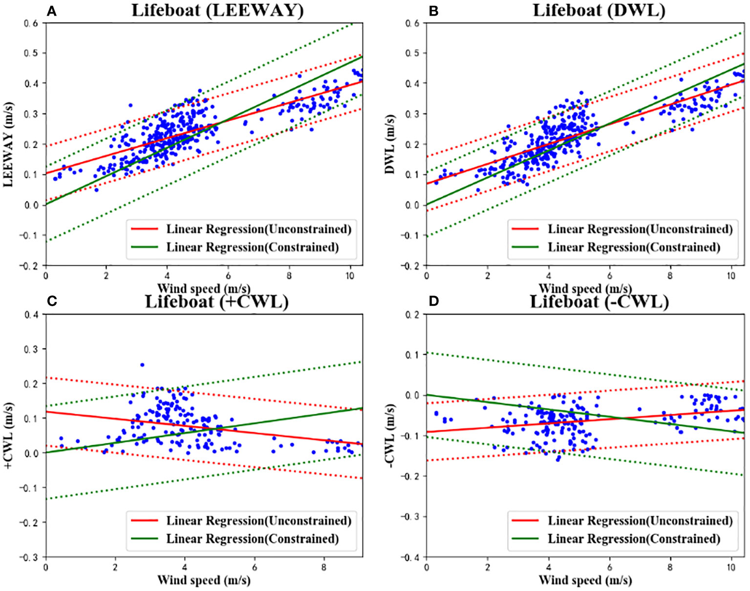
Figure 10 The linear regressions and 95% confidence level statistics of Leeway Speed (A), DWL (B), +CWL (C) and –CWL (D) with 10 m height wind speed for the improved drift model. Unconstrained linear regression (solid) and 95% of the confidence levels (dash) are plotted in red, while constrained linear regression is plotted in green.

Table 6 display the regression coefficients and standard errors for the open lifeboat’s improved drift model. Each leeway drift equation’s slope, intercept, and standard error of regression are represented by the regression coefficients a , b , and S_y/x, respectively. In the constrained and unconstrained cases, respectively, the R² values of DWL are 0.63 and 0.80.

TABLE 6

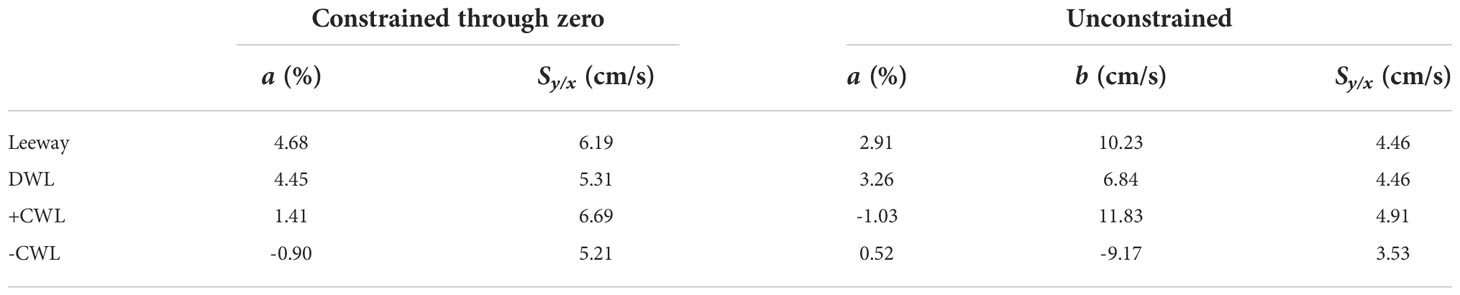
Table 6 The regression coefficients and standard errors of improved model.

Based on the outcomes of the unconstrained improved leeway coefficients in Table 6, the improved drift model expression for the open lifeboat is obtained as follows:

$$\{\begin{array}{c}{\overrightarrow{V}}_{lifeboat}={\overrightarrow{V}}_{lifeboat-x}+{\overrightarrow{V}}_{lifeboat-y}\\ V_{lifeboat-x}=0.9584V_{current-x}+L_x\\ V_{lifeboat-y}=0.9503V_{current-y}+L_y\end{array}\{\begin{array}{c}{L}_x=\left|\overrightarrow{L}\right|\times \cos (\theta )\\ L_y=\left|\overrightarrow{L}\right|\times \sin (\theta )\\ \overrightarrow{L}={\overrightarrow{L}}_d+{\overrightarrow{L}}_c\end{array}$$

where L_x is the x-direction component of$\overrightarrow{L}$, L_y is the y-direction component of$\overrightarrow{L}$, and θ is the angle between$\overrightarrow{L}$ and the positive x-direction. The expressions for${\overrightarrow{L}}_d$ and${\overrightarrow{L}}_c$ are as follows:

$$\{\begin{array}{c}{L}_d=3.26\%V_{wind}+6.84 cm/s; {\text{S}}_{\frac{y}{x}}=4.46 cm/s\\ L_{+c}=-1.03\%V_{wind}+11.83cm/s; {\text{S}}_{\frac{y}{x}}=4.91 cm/s\\ L_{-c}=0.52\%V_{wind}-9.17 cm/s; {\text{S}}_{\frac{y}{x}}=3.53 cm/s\end{array}$$

Comparisons and discussions

Two cases are set up to forecast the drift trajectories of the open lifeboat in order to compare and validate the accuracy of the three drift models. In Case 1, the ideal simulation conditions were adopted, with high quality data on the nearby wind and current, which were obtained through the drift observation experiments. In Case 2, we used operationally available data to run the drift models; the high frequency ground wave radar provided the current data, the wind data were provided by the continuous assimilation of wind field data from the ground wave radar through the Weather Research and Forecasting model (WRF). Based on the three models established in Section 4, the Lagrangian particle tracking method is used to run the simulated trajectories of the open lifeboat in Case 1 and Case 2. The calculation formula is referred to Eqs. (7)- (9) in Section 2.4.

The true drift trajectories of the open lifeboat in Case 1 and Case 2 and the simulated trajectories run by Lagrangian particle tracking method based on the three drift models are shown in Figures 11, 12. The actual drift distances are 13.95 km and 11.09 km, respectively. Figs. 11 and 12 show that the simulated trajectories are basically consistent with the true drift trajectories, and the simulated trajectories of the improved drift model are closest to the real trajectories. Table 7 lists the hourly and average distance differences between the lifeboat’s actual trajectory in Case 1 and the simulated trajectories of the three drift models. It shows that the distance deviations at 12 hours are 0.29 km, 0.25 km and 0.20 km, respectively. The prediction accuracy of the improved drift model is 31.0% higher than that of the dynamic drift model and 20.0% higher than that of the leeway drift model. The average distance deviations are 0.40 km, 0.39 km and 0.29 km, respectively. The prediction accuracy of the improved drift model is 27.5% higher than that of the dynamic drift model and 25.6% higher than that of the leeway drift model. Table 8 lists the hourly and average distance differences between the three drift models’ simulated trajectories and the actual trajectory of the lifeboat in Case 2. It shows that the distance deviations at 12 hours are 3.32 km, 3.58 km and 2.98 km, respectively. The prediction accuracy of the improved drift model is 10.2% higher than that of the dynamic drift model and 16.9% higher than that of the leeway drift model. The average distance deviations are 1.99 km, 2.35 km and 1.85 km, respectively. The prediction accuracy of the improved drift model is 7.0% higher than that of the dynamic drift model and higher by 21.3% than the leeway drift model. In conclusion, the improved drift model has higher prediction accuracy than both the dynamic drift model and the leeway drift model. In addition, the simulation results in case 1 are better than that in case 2, which is mainly due to the different data sources of wind and current.

FIGURE 11

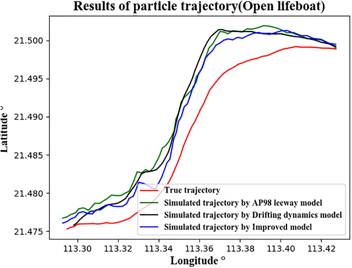
Figure 11 The true trajectory and the simulated trajectories using the Lagrangian particle tracking method for the open lifeboat in Case 1. The red line represents the true trajectory, and the green, black and blue lines represent the trajectories simulated by the leeway drift model, the dynamic drift model and the improved drift model, respectively.

FIGURE 12

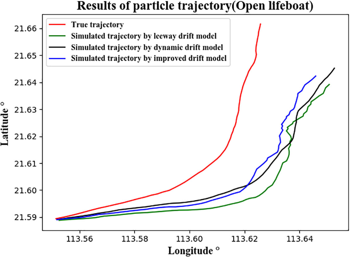
Figure 12 The true trajectory and the simulated trajectories using the Lagrangian particle tracking method for the open lifeboat in Case 2. The red line represents the true trajectory, and the green, black and blue lines represent the trajectories simulated by the leeway drift model, the dynamic drift model and the improved drift model, respectively.

TABLE 7

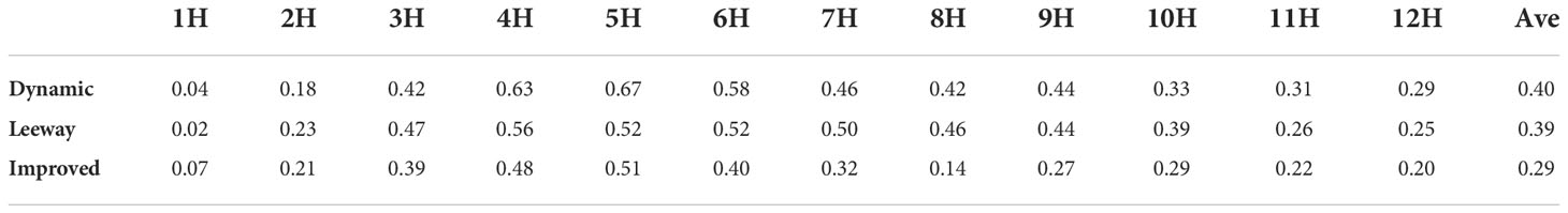
Table 7 The three simulated trajectories’ average and hourly distance deviations (km) were calculated by the Lagrangian particle tracking method and the true trajectory of open lifeboat in Case 1.

TABLE 8

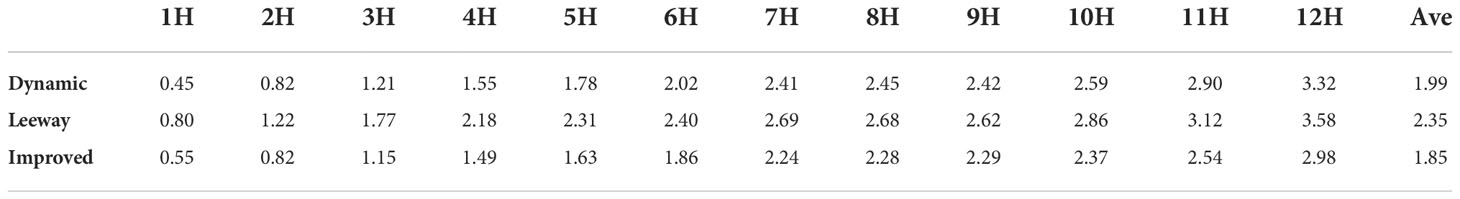
Table 8 The three simulated trajectories’ average and hourly distance deviations (km) were calculated by the Lagrangian particle tracking method and the true trajectory of open lifeboat in Case 2.

When using the Lagrangian particle tracking method to forecast the drift trajectories of the leeway model and the improved model, the crosswind leeway component of a single particle at a given moment can only be biased to the left or right. Although the POPC is set to 47.5%, the limitation of individual particle simulation still leads to small random variations in each trajectory simulation, which introduces random errors. To remedy this shortcoming, Monte Carlo technique can simulate the same trajectory using a sufficient number of particles and obtain the trajectory averaged after eliminating the error. As a result, 1000 particles were used in this article to simulate the lifeboat’s drift trajectory. In the simulation, not only 47.5% of the particle POPC was considered, but also 6% of the jibing frequency was added to the Monte Carlo simulation as an important influence factor. To assess the accuracy of the residual model and the improved model, 1000 random particles were processed with Eqs. (8) and (9). Each particle’s perturbation is based on Eqs. (10) - (12).

The Monte Carlo simulation results for Case 1 are shown in Figure 13. The hourly average and total average distance deviations between the two predicted trajectories in Case 1 and the true trajectory are recorded in Table 9. The results show that the average distance deviation in the 12th hour between the predicted trajectory of the improved drift model and the true trajectory is 0.20 km, which is smaller than that of predicted trajectory by the leeway model at 0.21 km. And the total average deviation of the improved trajectory is 0.42 km, which is also smaller than that of leeway trajectory at 0.46 km. This means that the improved drift model outperforms the leeway drift model in the Case 1 simulation.

FIGURE 13

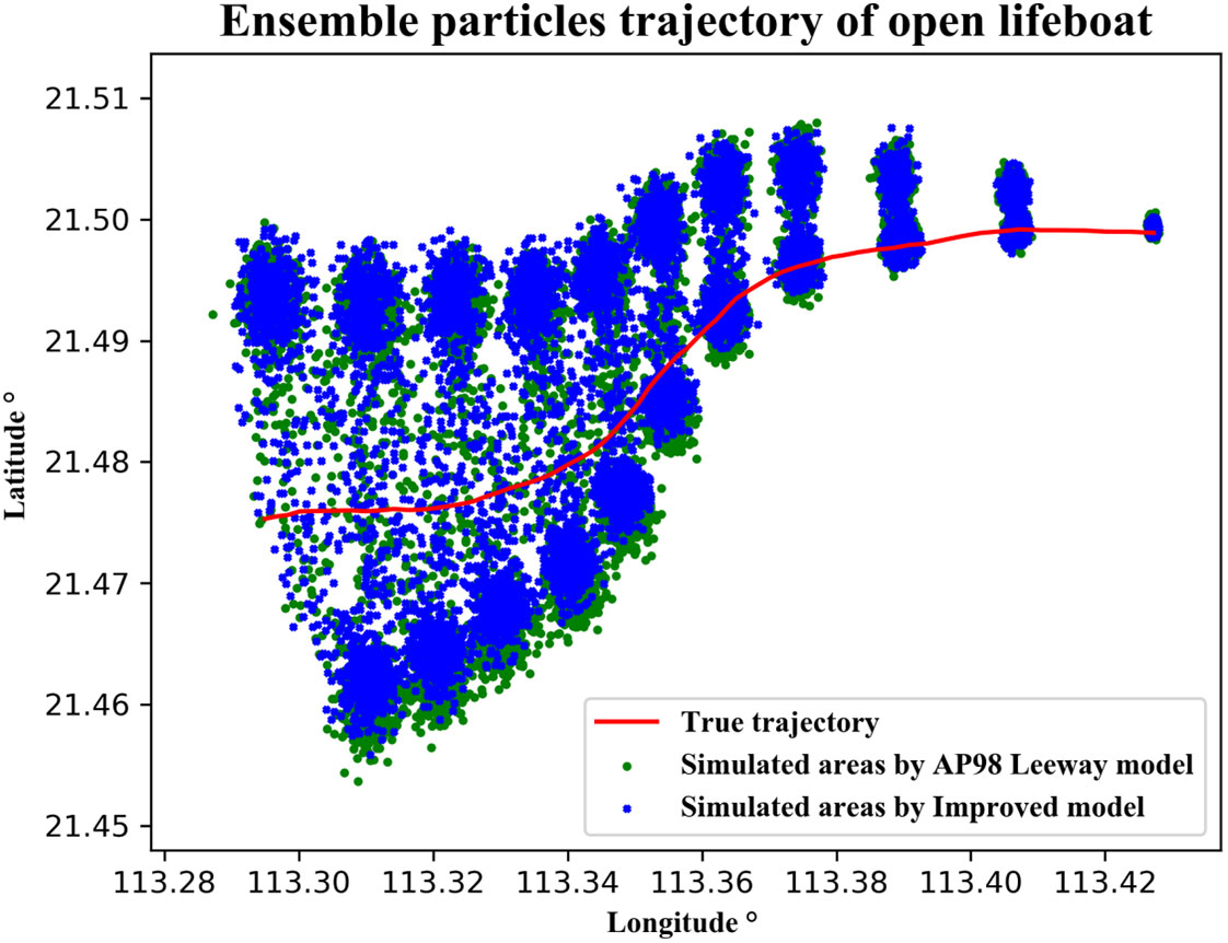
Figure 13 Monte Carlo simulation results for Case 1. The random particle distribution of hourly Monte Carlo simulation and the two predicted trajectories after particle averaging. The red line represents the true trajectory, and the two colors of green and black represent the leeway model and the improved model, respectively.

TABLE 9

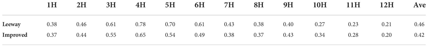
Table 9 Hourly average and total average distance deviations (km) between the particle distributions calculated by the Monte Carlo simulation and the true trajectory of open lifeboat in Case 1.

The Monte Carlo simulation results for Case 2 are shown in Figure 14. The hourly average and total average distance deviations between the two predicted trajectories in Case 2 and the true trajectory are recorded in Table 10. The results show that the average distance deviation in the 12th hour between the predicted trajectory of the improved drift model and the true trajectory is 3.26 km, which is smaller than that of predicted trajectory by the leeway model at 3.70 km. Additionally, the improved trajectory’s overall mean deviation is 2.09 km, which is also smaller than that of leeway trajectory at 2.42 km. The improved drift model’s simulation accuracy in this instance is also higher than the leeway drift model’s.

FIGURE 14

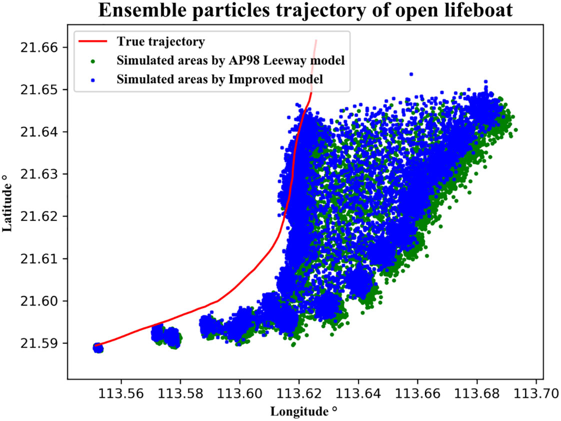
Figure 14 Monte Carlo simulation results for Case 2. The random particle distribution of hourly Monte Carlo simulation and the two predicted trajectories after particle averaging. The red line represents the true trajectory, and the two colors of green and black represent the leeway model and the improved model, respectively.

TABLE 10

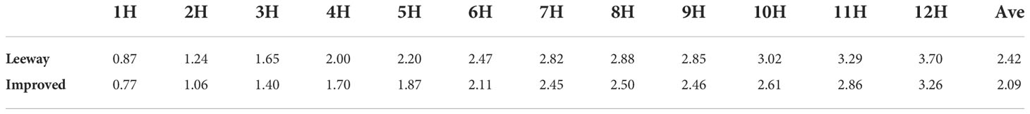
Table 10 Hourly average and total average distance deviations (km) between the particle distributions calculated by the Monte Carlo simulation and the true trajectory of open lifeboat in Case 2.

Similarly, in both case 1 and Case 2, the improved model shows better prediction performance. As the ideal simulation data is used in case 1 and the operationally available data is used in case 2, the prediction accuracy of case 1 is better than that of case 2.

Conclusion

The lifeboat is one of the most important life-saving equipment for escaping at sea when a ship is abandoned in an extreme emergency. The efficiency of maritime SAR operations can be enhanced by making precise prediction of the drift trajectories for lifeboats at sea. Three open lifeboats were subjected to a series of large-scale maritime drift experiments in the South China Sea in this study. The statistical results of the experiments show that the POPCs of the open lifeboat is 47.5%, the jibing frequency of the open lifeboat is 6% per hour, and the maximum leeway divergence angle is 45°. These drift characteristics are very important for the prediction of lifeboat drift trajectory. The leeway drift model, the dynamic drift model, and the improved drift model’s drift coefficients were obtained employing least squares fitting based on the experimental data. so as to establish the corresponding three drift prediction models. The Lagrangian particle tracking method and Monte Carlo simulations were used to assess the precision of the three models by two cases. The results show that the prediction accuracy of the improved drift model is higher than that of the dynamic drift model and the leeway drift model. Based on the above conclusions, it is recommended that the coefficients of the improved model can be directly used for search and rescue work in the South China Sea.

Data availability statement

The original contributions presented in the study are included in the article/Supplementary Material. Further inquiries can be directed to the corresponding authors.

Author contributions

LM and HT conceived the research. LM and KZ Supervised the research. LM, HT and XW Performed the research. KX, XW analyzed the data. LM, HT, KZ wrote the manuscript. All authors discussed the results and contributed to the final manuscript.

Funding

This work was supported by the National Key Research and Development Program of China (Grant No. 2021YFC3101800), National Natural Science Foundation of China (Grant No. U2006210), Shenzhen Science and Technology Program (Grant No. KCXFZ20211020164015024), Shenzhen Fundamental Research Program (Grant No. JCYJ20200109110220482).

Conflict of interest

The authors declare that the research was conducted in the absence of any commercial or financial relationships that could be construed as a potential conflict of interest.

Publisher’s note

All claims expressed in this article are solely those of the authors and do not necessarily represent those of their affiliated organizations, or those of the publisher, the editors and the reviewers. Any product that may be evaluated in this article, or claim that may be made by its manufacturer, is not guaranteed or endorsed by the publisher.

References

Allen A. A. (2005). “Leeway divergence (No. CG-D-05-05),” in Coast guard research and development center Groton CT. (Springfield, the National Technical Information Service).

Google Scholar

Allen A. A., Plourde J. V. (1999). “Review of leeway: field experiments and implementation (No. CG-D-08-99),” in Coast guard research and development center Groton CT. (Springfield, the National Technical Information Service).

Google Scholar

Allen A., Roth J., Maisondieu C., Breivik Ø., Forest B. (2010). Field determination of the leeway of drifting objects (Oslo, the Norwegian Meteorological Institute).

Google Scholar

Breivik Ø., Allen A. A. (2008). An operational search and rescue model for the Norwegian Sea and the north Sea. J. Mar. Syst. 69, 99–113. doi: 10.1016/j.jmarsys.2007.02.010

CrossRef Full Text | Google Scholar

Breivik Y., Allen A. A., Maisondieu C., Olagnon M. (2013). Advances in search and rescue at Sea. Ocean Dyn. 63 (1), 83–88. doi: 10.1007/s10236-012-0581-1

CrossRef Full Text | Google Scholar

Breivik Ø., Allen A. A., Maisondieu C., Roth J. C. (2011). Wind-induced drift of objects at sea: the leeway field method. Appl. Ocean Res. 33 (2), 100–109. doi: 10.1016/j.apor.2011.01.005

CrossRef Full Text | Google Scholar

Breivik Ø., Allen A. A., Maisondieu C., Roth J., Forest B. (2012). The leeway of shipping containers at different immersion levels. Ocean Dyn. 62 (5), 741–752. doi: 10.1007/s10236-012-0522-z

CrossRef Full Text | Google Scholar

Brushett B. A., Allen A. A., Futch V. C., King B. A., Lemckert C. J. (2014). Determining the leeway drift characteristics of tropical pacific island craft. Appl. Ocean Res. 44, 92–101. doi: 10.1016/j.apor.2013.11.004

CrossRef Full Text | Google Scholar

Brushett B. A., Allen A. A., King B. A., Lemckert C. J. (2017). Application of leeway drift data to predict the drift of panga skiffs: Case study of maritime search and rescue in the tropical pacific. Appl. Ocean Res. 67, 109–124. doi: 10.1016/j.apor.2017.07.004

CrossRef Full Text | Google Scholar

Brushett B. A., King B. A., Lemckert C. J. (2016). Assessment of ocean forecast models for search area prediction in the eastern Indian ocean. Ocean Modelling. 97, 1–15. doi: 10.1016/j.ocemod.2015.11.002

CrossRef Full Text | Google Scholar

Cucco A., Quattrocchi G., Satta A., Antognarelli F., De Biasio F., Cadau E., et al. (2016). Predictability of wind-induced sea surface transport in coastal areas. J. Geophys. Res. Oceans. 121, 5847–5871. doi: 10.1002/2016JC011643

CrossRef Full Text | Google Scholar

Daniel P., Marty F., Josse P., Skandrani C., Benshila R. (2003). Improvement of drift calculation in mothy operational oil spill prediction system. Int. Oil Spill Conf. Proc. 1, 1067–1072. doi: 10.7901/2169-3358-2003-1-1067

CrossRef Full Text | Google Scholar

Huang G., Law A. W. K., Huang Z. (2011). Wave-induced drift of small floating objects in regular waves. Ocean. Eng. 38, 712–718. doi: 10.1016/j.oceaneng.2010.12.015

CrossRef Full Text | Google Scholar

Ivić S., Crnković B., Arbabi H., Loire S., Clary P., Mezić I. (2020). Search strategy in a complex and dynamic environment: the MH370 case. Sci. Rep. 10, 19640. doi: 10.1038/s41598-020-76274-0

PubMed Abstract | CrossRef Full Text | Google Scholar

Kratzke T. M., Stone L. D., Frost J. R. (2010). “Search and rescue optimal planning system,” in Proceedings of the 13th International Conference on Information Fusion (FUSION), IEEE, Edinburgh, Scotland, United Kingdom. 1–8. doi: 10.1109/ICIF.2010.5712114

CrossRef Full Text | Google Scholar

Ličer M., Estival S., Reyes-Suarez C., Deponte D., Fettich A. (2020). Lagrangian Modelling of a person lost at sea during the Adriatic scirocco storm of 29 October 2018. Nat. Hazards Earth Syst. Sci. 20, 2335–2349. doi: 10.5194/nhess-20-2335-2020

CrossRef Full Text | Google Scholar

Liu Y., Weisberg R. H. (2011). Evaluation of trajectory modeling in different dynamic regions using normalized cumulative lagrangian separation. J. Geophys. Res. 116, C09013. doi: 10.1029/2010JC006837

CrossRef Full Text | Google Scholar

Röhrs J., Christensen K. H., Hole L. R., Broström G., Drivdal M., Sundby S. (2012). Observation-based evaluation of surface wave effects on currents and trajectory forecasts. Ocean Dyn. 62 (10-12), 1519–1533. doi: 10.1007/s10236-012-0576-y

CrossRef Full Text | Google Scholar

Serra M., Sathe P., Rypina I., Kirincich A., Ross S. D., Lermusiaux P., et al. (2020). Search and rescue at sea aided by hidden flow structures. Nat. Commun. 11 (1), 1–7. doi: 10.1038/s41467-020-16281-x

PubMed Abstract | CrossRef Full Text | Google Scholar

Xu Q. Q., Xiao W. J., Guan Q. L., Lu W. X. (2017). A parameter optimizing experiment of wind-induced velocity of rescuing floating object in the sea based on an observing project. Mar. Forecasts. 34 (02), 67–71. doi: 10.11737/j.issn.1003-0239.2017.02.009

CrossRef Full Text | Google Scholar

Yang Y., Tu H., Song L., Chen L., Xie D., Sun J. (2021). Research on accurate prediction of the container ship resistance by RBFNN and other machine learning algorithms. J. Mar. Sci. Eng. 9(4), 376. doi: 10.3390/jmse9040376

CrossRef Full Text | Google Scholar

Yulmetov R., Marchenko A., Loset S. (2016). Iceberg and sea ice drift tracking and analysis off north-east Greenland. Ocean. Eng. 123, 223–237. doi: 10.1016/j.oceaneng.2016.07.012

CrossRef Full Text | Google Scholar

Zhang J., Teixeira Â.P., Guedes Soares C., Yan X. (2017). Probabilistic modelling of the drifting trajectory of an object under the effect of wind and current for maritime search and rescue. Ocean Eng. 129, 253–264. doi: 10.1016/j.oceaneng.2016.11.002

CrossRef Full Text | Google Scholar

Zhou Y., Daamen W., Vellinga T., Hoogendoorn S. P. (2020). Impacts of wind and current on ship behavior in ports and waterways: A quantitative analysis based on AIS data. Ocean Eng. 213, 107774. doi: 10.1016/j.oceaneng.2020.107774

CrossRef Full Text | Google Scholar

Zhu K., Mu L., Tu H. (2019). Exploration of the wind-induced drift characteristics of typical Chinese offshore fishing vessels. Appl. Ocean Res. 92, 101916. doi: 10.1016/j.apor.2019.101916

CrossRef Full Text | Google Scholar