A practical pCO2 estimation and carbonate dynamics at an event of hypoxic water upwelling in Tokyo Bay

Urban bays have been considered to have a high CO₂ absorption function due to the high nutrient load and resultant primary production. It is expected to enhance the function by promoting a blue carbon policy co-beneficial with strengthening ecosystem services such as fisheries. Estimates of CO₂ absorption in urban bays have been based mostly on fragmentary information from shipboard observations, and an evaluation based on continuous observation of water quality is necessary considering the large spatiotemporal variability of such bay environment. In particular, Tokyo Bay has a specific feature of water pollution problem of hypoxia and anoxia leading to emitting high CO₂. Bottom hypoxic and anoxic waters develop from early summer to autumn in the central part of the bay and enclosed areas such as navigation channels and borrow pits. It is known that pCO₂ becomes very high in these waters, and their upwelling (called blue tide in the bay from the discoloration of the sea surface) is thought to cause high CO₂ emissions; however, the actual situation is unknown. We developed a practical method for continuous estimation of pCO₂ by appropriately combining continuous observation of water quality using sensors and measurements of carbonate parameters by water sampling. The results show that a highly reproducible and practical method for continuous estimation of pCO₂ was possible by combining in situ salinity and pH meters and the total alkalinity and calc. pH measured by a total alkalinity titrator for water samples. This method was then applied to the duration of blue tide that occurred in the head of the bay in the summer and autumn of 2021. The pCO₂ in the surface water was found to increase significantly and exceed 2000 µatm due to the upwelling of anoxic bottom water containing high pCO₂. Mean CO₂ emissions of approximately +2150 and +1540 µmol m^-2 h^-1 were observed at two stations during the upwelling period. The mean values rose to +2390 and +2190 µmol m^-2h^-1 with the blue tide and lowered to +810 and +1120 µmol m^-2 h^-1 without it, suggesting that high CO₂ emissions may occur due to upwelling, especially with blue tides.

1 Introduction

The enhancement of carbon removal was mentioned as a mitigation measure for climate change in the Paris Agreement in 2015. Blue carbon, defined as carbon sequestered and stored by marine ecosystems (Nellemann et al., 2009; Kuwae and Hori, 2019), has been attracting attention in this context. In coastal marine ecosystems, mangrove forests, salt marshes, seagrass meadows, and seaweed beds are considered significant carbon sinks (Breithaupt et al., 2012; Krause-Jensen and Duarte, 2016; Duarte and Krause-Jensen, 2017). Eutrophic urban bays have also been reported to contribute to a net carbon sink (Kuwae et al., 2016; Tokoro et al., 2021). Tokyo Bay, Japan, is a typical eutrophic urban bay with the Tokyo metropolitan area as its watershed. During the period of rapid economic growth from the 1960s, water pollution due to eutrophication became more serious, resulting in sediment organic pollution; the formation of bottom hypoxic and anoxic waters in summer and coastal upwelling of these waters lead to the mortality of benthic animals (Kodama and Horiguchi, 2011; Furukawa, 2015; Amunugama and Sasaki, 2018). To alleviate the problem, the Environment Agency (now the Ministry of the Environment) introduced a Total Pollutant Load Control System policy (TPLCS) in 1979, with COD as the target water quality item. Since 2001, total nitrogen and total phosphorus have been added as target items, achieving a significant decrease in pollutant loads (Tomita et al., 2016). By contrast, cultural oligotrophication caused by the TPLCS has been pointed out in recent years; it could be one of the causes of the significant decrease in fishery resources, including the impact on seaweed culture with the discoloration of edible larver (Yamamoto, 2003; Aoki et al., 2022). In addition, protecting coastal areas is becoming increasingly important to mitigate the growing severity of storm surge disasters associated with intensified typhoons due to climate change and tsunami disasters, raising expectations for green infrastructure (Sasaki et al., 2012; Liu et al., 2022). Environmental management of the bay must be thus reconsidered to realize a safe, beautiful, and abundant estuary, and there are growing expectations for blue carbon to contribute to enhancing these ecosystem services in a win–win relationship.

In Tokyo Bay, stratification appears from May to September due to increasing river runoffs and water temperatures. Extensive primary production lowers pCO₂ and contributes to the absorption of atmospheric CO₂ in the upper layer. The decomposition of organic matter increases dissolved inorganic carbon (DIC) and decreases pH, resulting in increasing pCO₂ in the lower layer. In addition, waters in navigation channels and borrow pits (mining sediments for the foreshore reclamation) in the inner part of the bay are extensively stagnant, causing the appearance of anoxic waters with high concentrations of sulfides (Sasaki et al., 2009a; Sasaki et al., 2009b). Although CO₂ is thought to be emitted to the atmosphere during coastal upwelling (Feely et al., 2008; Norman et al., 2013; Tokoro et al., 2021), the actual status of CO₂ emissions and DIC dynamics are not fully understood because coastal upwelling, as well as anoxia and hypoxia, is an episodic event in the bay (Sasaki et al., 2009b). Sulfate reduction becomes the main pathway for organic matter decomposition under anoxic conditions, resulting in sulfide accumulation in bottom waters. The sunlight scattering of particulate sulfur generated by sulfide oxidation during the upwelling is known as blue tides, in which the surface seawater turns milky blue (Otsubo et al., 1991; Higa et al., 2020). The DIC dynamics, including pCO₂ during blue tides, have not been well investigated. Although the upwelling of anoxic waters has been observed in other urban bays in Japan, such as Osaka Bay and Mikawa Bay, there have not been many reported cases worldwide (Gallardo and Espinoza, 2008; Minghelli-Roman et al., 2011; Schunck et al., 2013; Ma et al., 2021). However, the global trend of expansion of hypoxic waters due to climate change and the effects of upwelling of such waters are considered problematic; knowledge on CO₂ emissions associated with the upwelling of hypoxic and anoxic waters is considered essential (Diaz and Rosenberg, 2008; Vaquer-Sunyer and Duarte, 2008; Gilbert et al., 2010; Testa et al., 2017; Breitburg et al., 2018; Lee et al., 2018; Hong et al., 2022; Pearson et al., 2022). Direct and continuous measurements of air–seawater CO₂ fluxes have been made using eddy covariance (Zemmelink et al., 2009; Tokoro et al., 2014) and floating chamber methods (Tokoro et al., 2007; Tokoro et al., 2014); these are, however, generally costly and present many challenges for practical deployment. Therefore, the bulk method is widely employed to estimate the CO₂ fluxes. When applying the bulk method, it is necessary to estimate the pCO₂ in seawater. The method of analyzing water samples using a total alkalinity titrator is versatile, reliable, and widely used (Dickson et al., 2007; Tokoro et al., 2014). There are also estimation methods that combine salinity and pH from shipboard or mooring observations (Johnson et al., 2016; Williams et al., 2016; Williams et al., 2017). However, there is no universal formula, and developing an appropriate estimation method for each environment is essential. Other methods for estimating surface seawater pCO₂ include using satellite imagery (Stephens et al., 1995; Sarma et al., 2006; Lohrenz et al., 2019; Mohanty et al., 2022) and a combination of satellite imagery with field observations using statistical methods based on multivariate analysis and machine learning (Lefévre et al., 2005; Friedrich and Oschlies, 2009; Signorini et al., 2013; Majkut et al., 2014; Moussa et al., 2016; Benallal et al., 2017). Although these are considered adequate for evaluation in a wide area, applying them to episodic coastal upwelling events with a narrow band of affected areas along the coastline is challenging.

Several continuous monitoring stations for water quality are currently operated in Tokyo Bay by the Ministry of Land, Infrastructure, Transport and Tourism (MLIT); some of the water quality parameters necessary for estimating pCO₂ have been continuously observed. Estimating continuous pCO₂ based on such monitoring will enable continuous monitoring of carbon absorption and emission, including during episodic events, which is expected to arouse public interest in environmental management and policy implementation for strengthening blue carbon with the co-benefits of enhanced ecosystem services in urban bays. We hypothesize that continuous measurement using water quality sensors in combination with periodic calibration by water sampling will enable continuous observation of pCO₂ with reasonable accuracy for each specific estuarine and coastal water. This study aims to develop a practical method for continuously estimating pCO₂ from measured water quality parameters using moored sensors combined with water sampling analysis using a total alkalinity titrator and clarify DIC dynamics, including pCO₂, during the upwelling of anoxic waters in Tokyo Bay.

2 Materials and methods

2.1 Study area

Tokyo Bay is a eutrophic semi-enclosed estuarine embayment surrounded by the Tokyo metropolitan area, with major and minor lengths of approximately 60 and 20 km and a mean depth of 17 m (see Figure 1). Major rivers flow into the bay from the western coast, and stratification develops from spring to autumn. Appearance of hypoxia and anoxia in the bottom waters between spring and autumn has been a serious water quality problem causing mortality of fishes and benthic animals in tidal flats and shallow water areas. The bottom anoxic waters often contain hydrogen sulfide generated by sulfate reduction (Kodama and Horiguchi, 2011; Furukawa, 2015; Amunugama and Sasaki, 2018). In addition, navigation channels and borrow pits (dredged for the foreshore reclamation) exist at the bay head, in which anoxic waters with a high concentration of hydrogen sulfide often appear (Sasaki et al., 2009a; Sasaki et al., 2009b). The upwelling of such anoxic waters causes discoloration of surface water due to the oxidation of hydrogen sulfide generating particulate sulfur, which scatters the sunshine and the surface watercolor turned to milky blue called blue tide in Tokyo Bay (Otsubo et al., 1991; Sasaki et al., 2009b; Higa et al., 2020; Wang et al., 2022).

FIGURE 1

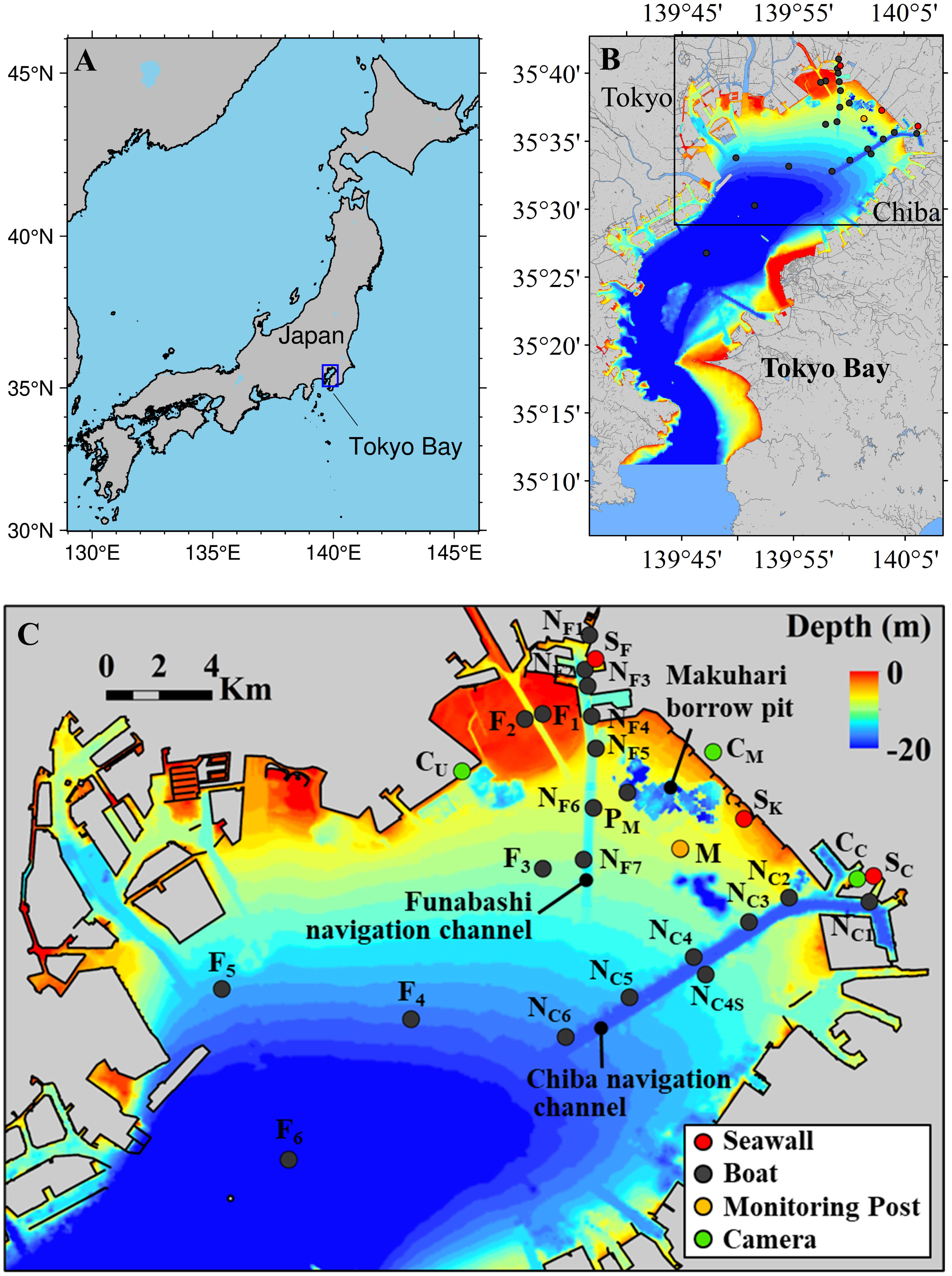
Figure 1 Map of Tokyo Bay with observation stations. (A) Location of Tokyo Bay in Japan. (B) The whole of Tokyo Bay. (C) Northern part of Tokyo Bay corresponding to the box in (B) with observation stations. The red filled circles of Stns. S_F, S_K, and S_C are buoy stations for continuous water quality monitoring adjoining to the seawall in Funabashi, Kemigawa, and Chiba, respectively. The gray filled circles are boat cruising stations: Stns. F₁ to F₆ are in flat bottoms; Stns. N_F1 to N_F7 are in the Funabashi navigation channel; N_C1 to N_C6 are in the Chiba navigation channel; Stn. P_M is in the off-Makuhari borrow pit. The green filled circles of Stns. C_U, C_M, and C_C are the fixed camera monitoring stations for observing seawater color at Urayasu, Makuhari, and Chiba, respectively. The yellow filled circule of Stn. M is a water quality monitoring station managed by MLIT.

2.2 Field observation

We conducted an observation of water quality to identify carbonate processes at an event of blue tide at the bay head. Observation stations were deployed as shown in Figure 1C. Stns. S_F, S_K, and S_C are buoy stations for continuous water quality monitoring adjoining to the seawall in Funabashi, Kemigawa, and Chiba, respectively. Stns. with initials of F, N, and P are observation stations using a boat at the flat bottom, the Funabashi and Chiba navigation channels, and the off-Makuhari borrow pit. Stns. with initials C are the fixed camera monitoring stations to observe the occurrence of blue tides. Stn. M is a water quality monitoring station managed by MLIT.

2.2.1 Observation at buoy monitoring stations

We conducted continuous measurements of water quality at 10-min intervals using self-recording sensors attached to buoys at Stns. S_F (August 27–September 17), S_K (August 31–September 10), and S_C (August 27–September 10) adjoining to the seawalls at Funabashi, Kemigawa, and Chiba to observe the upwelling processes of hypoxic and anoxic waters (see Figure 1C). The sensors were deployed at the surface and bottom at Stns. S_F and S_c, and at the surface, middle, and bottom at Stn. S_K. The water depth is about 4–5.5 m at Stn. S_F, about 7–9m at Stn. S_K, and about 4–6m at Stn. S_C. The measured items at each depth and station were the water pressure (CO-U20L-04/02, HOBO), temperature and salinity (ACTW-CMP, JFE Advantech), turbidity (ACTW-CMP, JFE Advantech), and dissolved oxygen (DO) (CO-U26-001, HOBO, or ADOW-CMP, JFE Advantech). A pH sensor (CO-MX2501, HOBO) was installed only at the surface at each station.

We visited the continuous monitoring stations and measured the vertical profiles of multiparameter water quality of temperature, salinity, turbidity, DO, and pH using a throw-in water quality meter (AAQ-RINKO 177, JFE Advantech) on September 1, 2, 3, and 10 at the three stations. In addition, we conducted the measurements on August 27 and September 17 at Stn. S_F, on August 31 at Stn. S_K, and on August 27 at Stn. S_C. We also took water samples at each depth at the three stations using a 1300 mL RIGO-B water sampler (5023-A, Rigo-sha) on the same days. Furthermore, only surface water samples were collected using a bucket at the three stations on September 8. A 50% saturated solution of mercury (II) chloride was added to the water samples in Duran bottles at twice the standard dosage range for saturated solutions (0.02–0.05%) for measuring pH, TA, and DIC following Dickson (2007). Water samples to be analyzed for sulfide concentrations were poured into 100 mL brown bottles, immediately fixed by adding three granular sodium hydroxides to make them alkaline with a pH of about 12. These samples were immediately taken back to the laboratory and stored in the dark at room temperature.

2.2.2 Observation using a boat

Water quality observation using a boat was carried out at stations with initials F, N, and P in Figure 1C in the inner part of the bay for collecting offshore data on July 16, August 20, September 16, October 12, and October 19. Measurements of the vertical profile of the same multiparameter water quality were conducted using a throw-in water quality meter (AAQ-RINKO 177, JFE Advantech) with an interval of 0.1 m. Water samples were collected using a 6000 mL of Van Dorn water sampler (5026-C, Rigo-sha) at the surface, middle, and bottom. The water samples were pre-processed following the same method described in the previous subsection.

2.2.3 Fixed camera monitoring

In order to capture the occurrence of blue tides at the bay head, we used high-rise towers of C_U (Tokyo Bay Tokyu Hotel, 60 m height, 35;38;18N 139;55;54E), C_M (APA Hotel & Resort Tokyo Bay Makuhari, 183.1 m height, 35;38;36N 140;2;12E), C_C (Chiba Port Tower, 125.2 m height, 35;36;0N 140;5;54E) and a fixed-point camera (SP108-J, HykeCam or KG770, Keep Guard) were installed on the roof of each of the three towers and at the mooring observation points. Interval photography of the sea surface was conducted at 5-min intervals between sunrise and sunset.

2.2.4 Collecting archived data of MLIT

We collected a dataset of vertical profiles of hourly water quality at Stn. M (35;36;39N 140;1;24E) acquired by the website of MLIT. The items of temperature, salinity, turbidity, chlorophyll a, and DO were available at 1 m intervals, whereas pH was available only at the surface, middle, and bottom.

2.3 Analysis of carbonate parameters

For the analysis of TA and DIC of the water samples, hydrochloric acid titration was performed using a total alkalinity analyzer (ATT-05, Kimoto Electric Co., Ltd.). A closed-cell method, in which acid titration is performed in the presence of carbonate in seawater, was selected as the measurement method. This method focused on the relationship between the changes in DIC and TA due to hydrochloric acid titration. DIC and TA are determined based on the standard potential E0, which maximizes the coefficient of determination of the single regression equation in this relationship, and K1Factor, which is related to the acid dissociation constant. The DIC and TA are determined based on the standard potential E0 and the K1Factor related to the acid dissociation constant that maximize the coefficient of determination of the single regression equation in this relationship. By giving this optimum E0 to Nernst’s equation, the pH before hydrochloric acid titration (calc. pH) is obtained. This calc. pH was used when calculating pCO₂, which is described later. During the analysis, the temperature in the laboratory was adjusted to approximately 20°C by air conditioning.

2.4 Estimation of TA using salinity

Since there is a strong correlation between TA and salinity, we considered a method to estimate TA from salinity. To obtain a continuous estimate of TA from salinity measured in our field observation and collected by MLIT, we examined the correlation between the salinity and TA of the water samples. Figure 2 shows the relationships between TA and salinity measurements for (A) all water samples and (B) for the samples shallower than 10 m, and (C) the residual from the measured TA and the estimated TA by the regression for samples shallower than 10 m. There was a positive highlinear correlation between TA and salinity of all water samples except in the high-salinity range where TA values deviated significantly, taking higher than 2500 µmol/kg, and low-salinity range. The outliers in the high-salinity range were sampled deeper than 18 m in the borrow pit (Stn. P_M) under anoxic conditions. As shown in the middle panel of Figure 2B, the relationship between TA and salinity at depths shallower than 10 m was better fitted, which was used further in the present study. There was, however, one outliner in the lowest salinity of around 17 PSU. This sample was taken from the surface water at the far end of the Funabashi navigation channel (Stn. N_F3) on August 24 under normal conditions without upwelling, where the influence of river discharge was significant. There may be a limitation in estimating TA from salinity under low-salinity conditions directly influenced by river discharges.

FIGURE 2

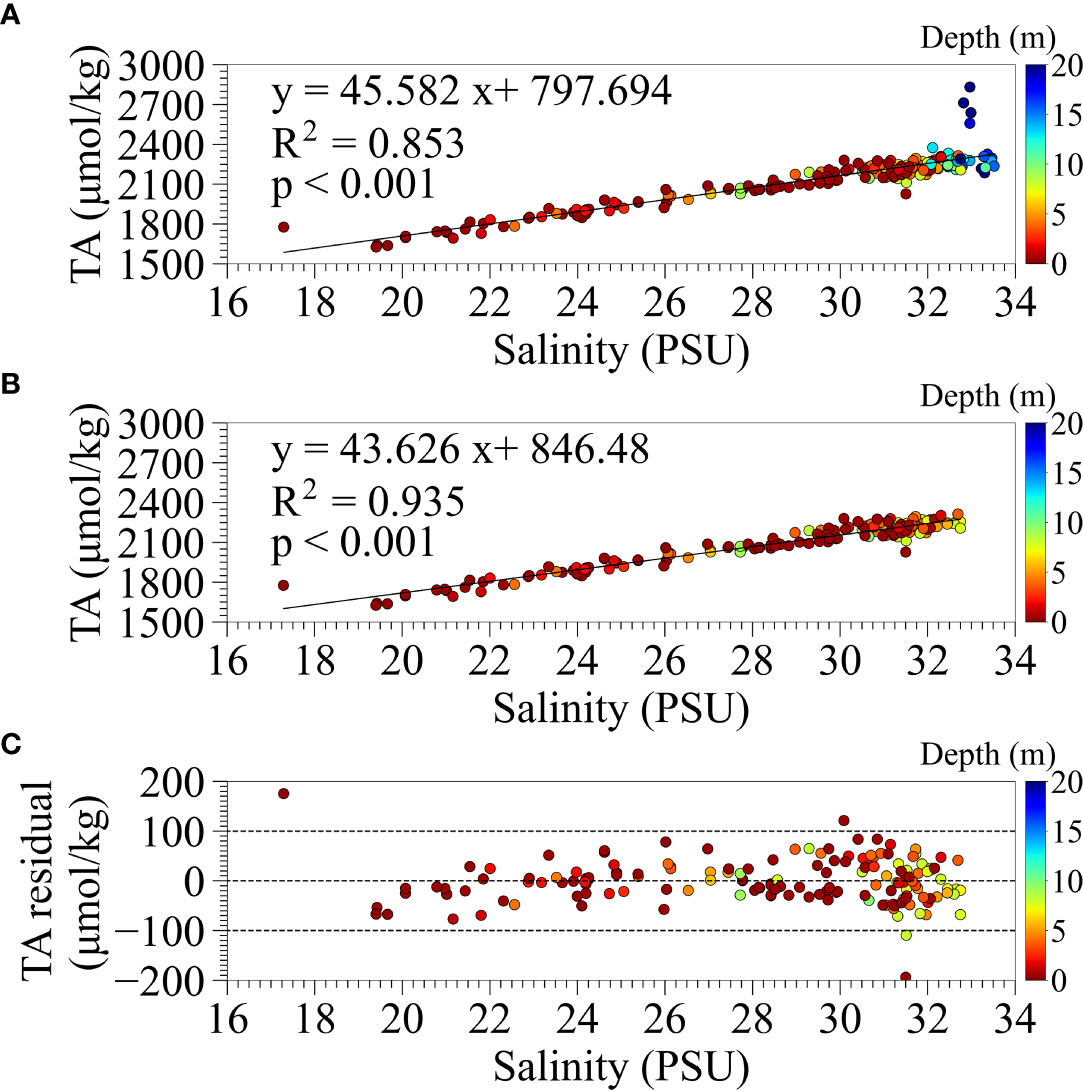
Figure 2 The relationship between TA and salinity measurements for (A) all water samples and (B) for samples shallower than 10 m in depth. (C) The residual from the measured TA and the estimated TA by the regression equation for samples shallower than 10 m in depth.

2.5 Estimation of pCO₂

pCO₂ for each water sample was calculated using PyCO2SYS (Humphreys et al., 2022) from TA analysis values and calc. pH by ATT-05. We activated the option of the influence of sulfide as some samples contained sulfide generated under the anoxic condition. The required water temperature and salinity as input parameters were given as observed values at the time that the samples were taken. Among several choices for the values of parameters such as equilibrium constants, we selected the total scale for pH scale, Mojica Prieto and Millero (2002) for K₁ and K₂, Dickson (1990) for KHSO4, Lee et al. (2010) for B_T, and Dickson and Riley (1979) for KHF were selected. For samples in which sulfide ions were detected, pCO₂ was calculated taking sulfide concentrations into account.

Continuous pCO₂ was calculated using PyCO2SYS from continuously estimated TA using measured salinity explained in subsection 2.4 and measured pH. The adopted parameters and their values for PyCO2SYS were the same as those for water samples. The estimated pCO₂ were, however, found to be inconsistent with those of the corresponding water samples. As the major cause of the inconsistency was considered due to a bias of the continuously measured pH values, we developed a correlation equation between calc. pH obtained by ATT-05 under stable environmental conditions and the measured pH.

2.6 Estimation of CO₂ flux between the atmosphere and seawater

The commonly adopted bulk equation (1) was used to calculate the continuous CO₂ flux (F_CO2) between the atmosphere and seawater at Stns. S_F, S_K, S_C, and Stn. M, where continuous water quality measurements were conducted.

$\begin{array}{ll}{F}_{\text{CO}2}=k{K}_0\left(p{\text{CO}}_{2\text{sw}}-p{\text{CO}}_{2\text{air}}\right)& (1)\end{array}$

where K₀ is the solubility equilibrium constant for CO₂ (mol atm^-1 kg^-1) using the formula (Weiss, 1974); pCO_2sw and pCO_2air are pCO₂ (µatm) in the surface water and atmosphere, respectively, and k is the piston velocity (cm/h) estimated by the following formula proposed by Wanninkhof (2014) updating that by Wanninkhof (1992);

$\begin{array}{ll}k=0.251\times U_{10}^2{\left(\frac{S_c}{660}\right)}^{-0.5}& (2)\end{array}$

where U₁₀ is the wind speed at 10 m above the sea surface at Stn. M, and S_C is the Schmidt number for CO₂ (Jähne et al., 1974). Although the piston velocity may also be influenced by the current velocity and depth (Call et al., 2015), we did not consider them as the current velocity was not measured. The adopted formula may be acceptable supposing that the wind speed may influence more significantly than the current velocity as the observation was conducted at the bay head, where the current velocity is relatively weak. The pCO_2air was given as a constant (470 ppm) averaged over the shipboard observations on September 16, 2021, which was converted to pCO_2air by subtracting the vapor pressure at the Chiba Meteorological Observation Station, Japan Meteorological Agency. Following Orr et al. (2018) and using PyCO2SYS, we estimated propagated uncertainties for the CO₂ flux supposing the standard uncertainties for TA and pH of ATT-05 to be 2 µmol/kg and 0.01, respectively.

3 Results

3.1 Observed water quality at Stn. M by MLIT and occurrences of blue tide

Figure 3 shows the time series of observed wind vectors with the durations of blue tide occurrences, tidal heights, and water quality parameters at Stn. M from June to October 2021. The durations of blue tide occurrences were identified by visual and camera monitoring of sea color changes during field observations and as reported by Chiba Prefecture. The occurrences of blue tides in the inner part of Tokyo Bay were identified six times from mid-June to late October in 2021. Blue tides occur due to the upwelling of anoxic water containing hydrogen sulfide caused by the offshore-ward wind-driven current caused by the north-eastward wind. The scale and duration of the blue tides are related to the magnitude of the anoxic water mass prior to the onset and the wind direction and speed during the blue tide. The blue tides in early summer (June 17) and mid-autumn (October 14) before and after the strong stratification and those (June 29 and July 27) during typhoon approaching were small and ceased within a couple of days due to the extensive water mixing. On the other hand, the blue tide from September 2 to 9 was the largest in 2021 caused by northerly weak continuous winds lasted for more than 1 week.

FIGURE 3

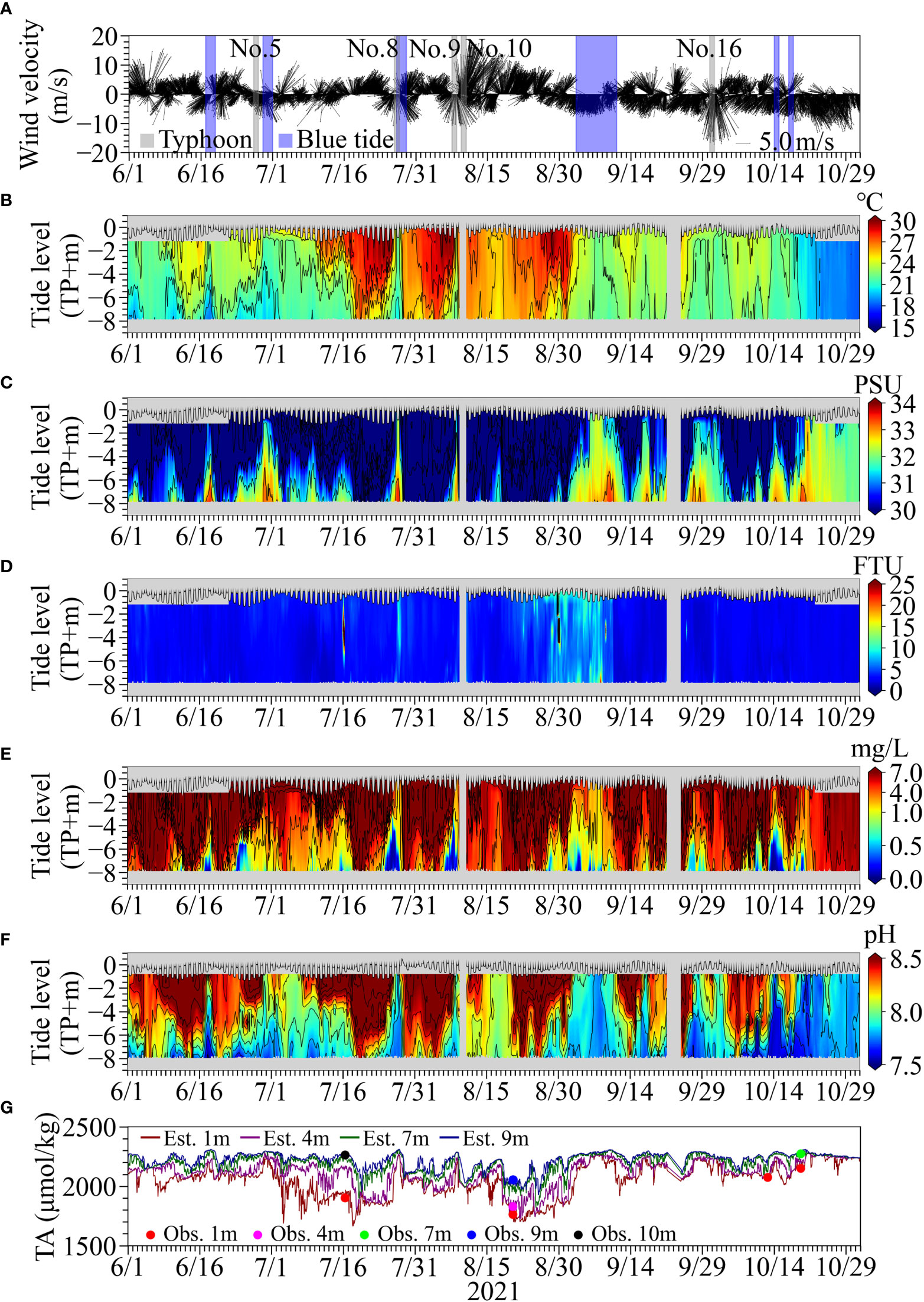
Figure 3 (A) Time series of observed wind vectors with the durations of the occurrences of blue tide (hatched in blue) and the events of typhoon approaching (hatched in gray). The time series of vertical profiles of (B) temperature, (C) salinity, (D) turbidity, (E) DO, and (F) pH, with tide level. (G) The time series of estimated TA using continuously observed salinity and measured TA using ATT-05 for water samples.

Sudden decrease in temperature and increase in salinity were observed when this largest blue tide occurred, which reflects the upwelling of the offshore dense bottom water. The turbidity became high, indicating the generation of particulate sulfur due to the oxidation of sulfide. DO and pH became lower as hypoxic and anoxic waters approached Stn. M.

The variation in TA was similar to that in salinity; higher TA was observed in deeper water. TA tended to become high and uniform in the vertical when the upwelling events occurred. The difference between the TA measured using ATT-05 minus the TA estimated from continuously observed salinity at nearby depths ranged from −27.2 µmol/kg to 4.4 µmol/kg (N = 6) at the surface, −48.0 µmol/kg (N = 1) at a depth of 4m, −68.0 µmol/kg (N = 1), −28.8 µmol/kg to 14.7 µmol/kg (N = 2) at 9-m depth, and −0.6 µmol/kg (N = 1) at 10-m depth. Although the estimated TA tended to be slightly higher than the observed values, the estimated TA values were generally consistent with the measured TA using ATT-05 for the corresponding water samples, suggesting the validity of the TA estimation method.

The blue tide occurred in early September was observed at our observation stations in the bay head. Figure 4 shows fixed camera photos at (A) Chiba Port (C_C), (B) Makuhari (C_M), and (C) Urayasu (C_U). Generally, blue tides in the bay are initiated by the upwelling of anoxic waters in the Funabashi and Chiba navigation channels due to the continuous blowing of northeasterly winds. The upwelling of the offshore bottom waters expands the blue tide area along the coast of the bay head. The intrusion of the offshore bottom waters with high density also causes pushing out the anoxic waters in borrow pits, thus enhancing the blue tide. Blue tides are often terminated by strong winds or a change in the wind direction, promoting mixing and dispersion of the blue tide waters. Our observed blue tide followed a similar pattern but lasted longer than usual due to persistent light northeasterly winds.

FIGURE 4

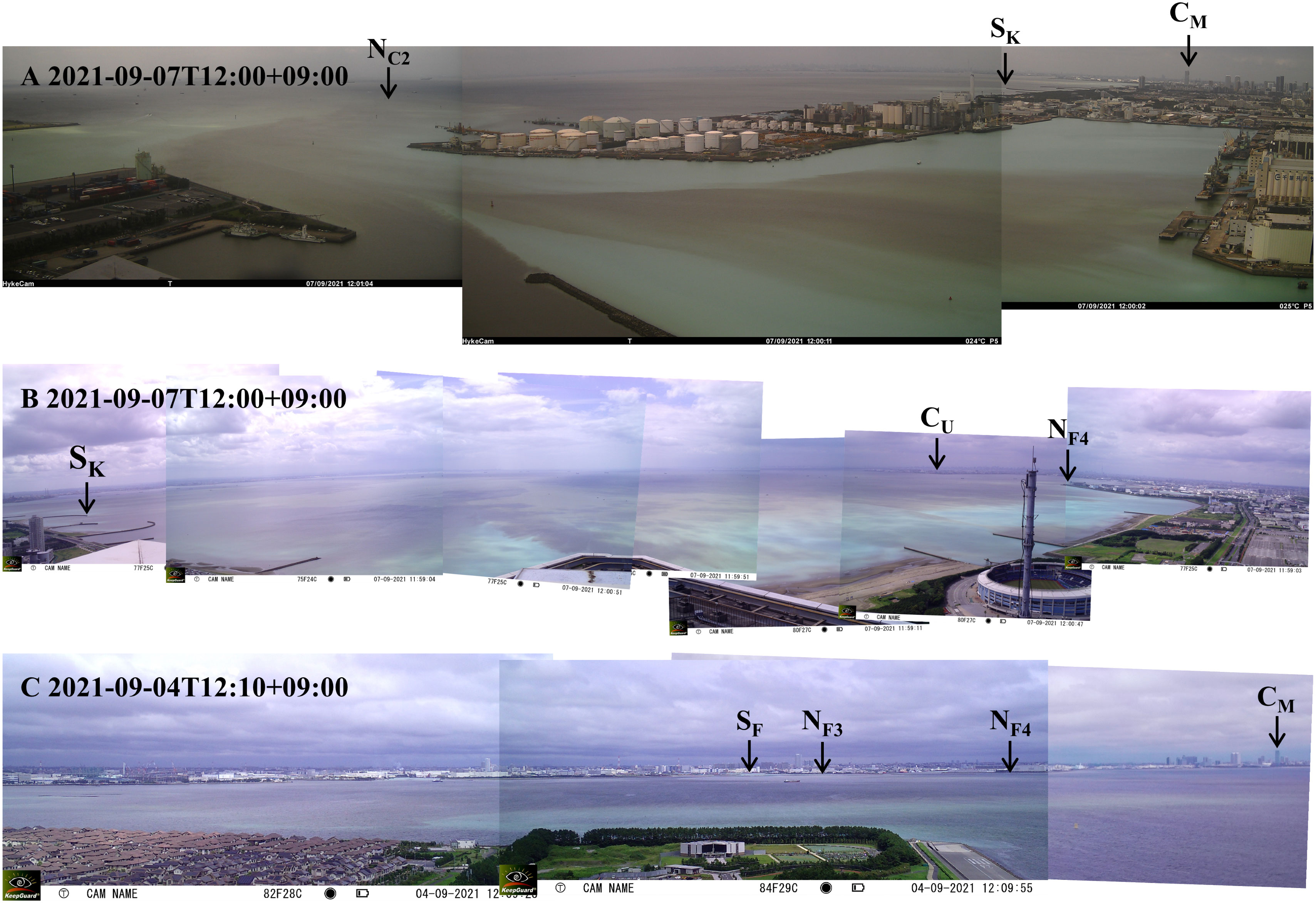
Figure 4 Fixed camera photos of the occurrence of blue tide in early September at (A) Stn. C_C, (B) Stn. C_M, and (C) Stn. C_U. The locations of some stations are specified in the photos.

3.2 Vertical profiles of water quality in navigation channel and borrow pit

Figures 5, 6 show that under normal conditions in August before the outbreak of blue tide, pCO₂ in the surface water was significantly less than 400 µatm, much lower than pCO₂ in the atmosphere, indicating the bay at the stations being the absorber of CO₂ under the stratified condition (Figures 5A, B, 6A–D). The TA values in the surface layer at this time were larger than those of the DIC, ranging approximately from 200 µmol/kg to 500 µmol/kg.

FIGURE 5

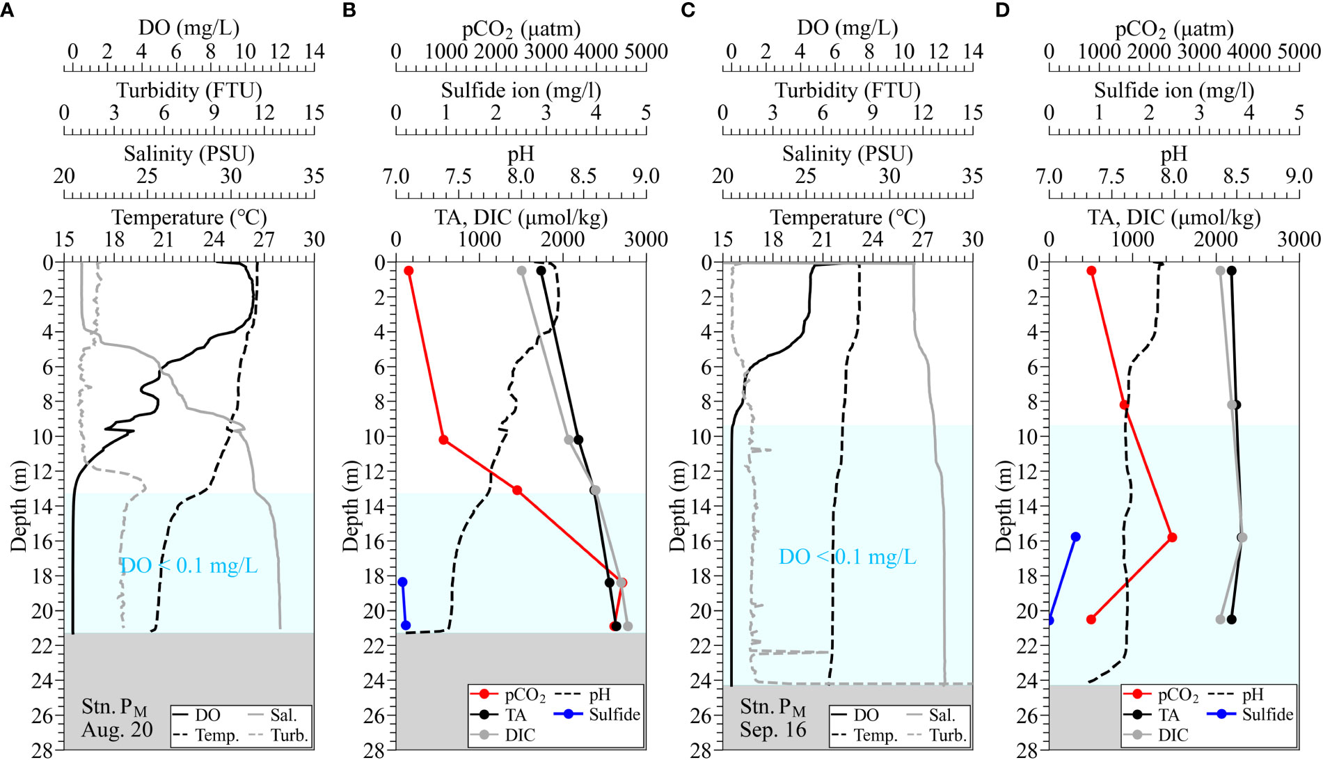
Figure 5 Observed vertical profiles of water quality of temperature, salinity, turbidity, DO, and pH using AAQ-RINKO, measured TA, DIC, total sulfide for water samples, and estimated pCO₂ at the borrow pit (Stn. P_M). Panels (A, B) are under normal conditions on August 20; panels (C, D) are during the upwelling on September 16. Hatched boxes in light blue denote hypoxic water with DO of below 0.1 mg/L.

FIGURE 6

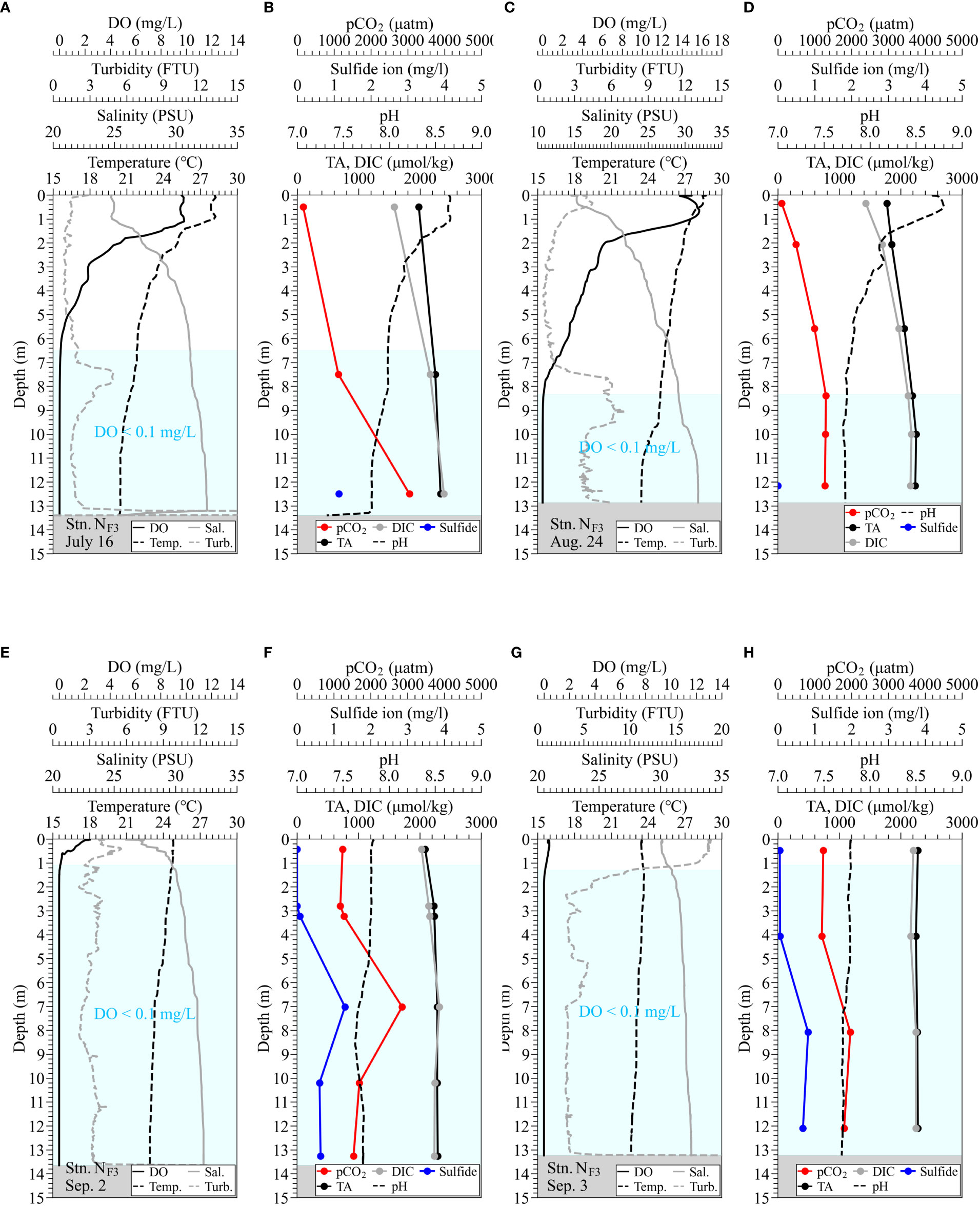
Figure 6 Observed vertical profiles of water quality of temperature, salinity, turbidity, DO, and pH using AAQ-RINKO, measured TA, DIC, and total sulfide for water samples, and estimated pCO₂ at the Funabashi navigation channel (Stn. N_F3). Panels (A, B) are under normal conditions on July 16; panels (C, D) are under normal conditions on August 24. Panels (E, F) are during the upwelling on September 2; panels (G, H) are during the blue tide on September 3. Hatched boxes in light blue denote hypoxic water with DO below 0.1 mg/L.

At the borrow pit (Stn. P_M), pCO₂ increased with increasing depth approximately from 1000 µatm at a depth of 10 m to greater than 4000 µatm at the bottom, where the waters were rather stagnant (Figures 5A, B). These pCO₂ were much higher than those in the atmosphere, suggesting potential high CO₂ emission to the atmosphere when these waters upwell. The difference between TA and DIC showed a decreasing trend, and DIC was higher than TA in the bottom layer, with a difference of more than 130 µ mol/kg. Although a similar trend was observed at the Funabashi navigation channel (Stn. N_F3), the pCO₂ in the bottom water varied significantly from approximately 3000 µ atm on July 16 to less than 1300 µatm on August 24 (Figures 6A–D). The waters in the navigation channel is considered more easily mobile than those in the borrow pit, resulting in a large variation in pCO₂. In contrast, the bottom layer pCO₂ at the flat bottom (Stn. M) with 10 m deep was around 1000 µatm, lower than the bottom waters at Stns. P_M and N_F3 under normal conditions. However, pCO₂ in the bottom waters at the flat bottom was still much higher than that in the atmosphere, which is also considered causing potential large CO₂ emission.

The density stratification disappeared due to the occurrence of upwelling, and the upper layer became hypoxic in September 2 (Figures 6E–H). In the surface layer, turbidity increased with the onset of blue tide, and pCO₂ in the surface layer increased to approximately 1200 µatm at Stn. N_F3 on September 3. The pCO₂ on September 2 was the maximum value of just under 3000 µatm observed in the middle layer.

3.3 Observed continuous water quality during blue tide

At Stn. S_F, the surface layer became anoxic on September 2 and continued until September 11 (Figure 7A). The slight increase in DO observed on September 5 was found to correspond to the weakening of the discoloration of the surface water caused by the blue tide according to the fixed camera photos. A decrease in DO was also observed after September 15, which was considered a reoccurrence of upwelling associated with the northerly wind, but did not lead to a significant blue tide (Figure 7A).

FIGURE 7

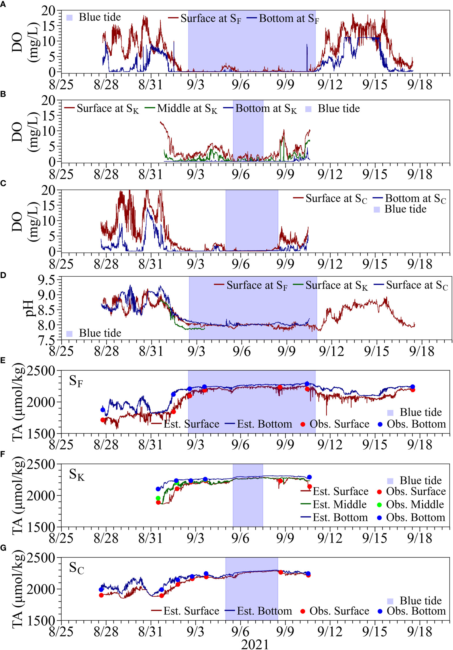
Figure 7 Time series of water quality at Stns. S_F, S_K, and S_C. Top three panels are observed DO at the surface and bottom, at (A) Stn. S_F, (B) Stn. S_K, and (C) Stn. S_C. Panel (D) shows observed surface pH. The bottom three panels are observed (solid lines) and estimated (filled circles) TA at the surface and bottom at (E) Stn. S_F, (F) Stn. S_K, and (G) Stn. S_C.

At Stn. S_C, anoxia of the surface water was observed from around September 3, delayed by the Stn. S_F, and a temporary increase in DO was observed on September 4, which continued until the afternoon on September 8 (Figure 7C). At Stn. S_K, hypoxia in the surface water was observed from the afternoon on September 5, which did not lead to anoxia. The pH in the surface water during the onset of the blue tide decreased from 8.0 to 7.8 at Stn. S_F while remained at about 8.0 at Stn. S_C (Figure 7D). At Stn. S_K, although the recording was stopped midway due to a malfunction of the pH meter, the pH was found to drop below 7.9. The respective differences in TA measured using the ATT-05 in the surface and bottom layers minus TA estimated from continuously observed salinity ranged from −193.9 µmol/kg to 83.7 µmol/kg (N = 8) and from −0.65 µmol/kg to 63.5 µmol/kg (N = 6) at Stn. S_F, from −48.8 µmol/kg to 30.9 µmol/kg (N = 6) and from −19.0 µmol/kg to 20.9 µmol/kg (N = 5) at Stn. S_K; from −50.4 µmol/kg to 54.1 µmol/kg (N = 7) and from −9.5 µmol/kg to 63.7 µmol/kg (N = 6) atStn. S_C (Figures 7E–G). The TA values at Stn. S_F in the surface and bottom waters were approximately 1700 and 2000 µmol/kg before the occurrence of blue tide, showing a difference between the surface and bottom. During the onset of the blue tide, TA in both the surface and bottom waters increased; the difference between them became smaller, ranging from 2200 to 2300 µmol/kg. After September 10, TA showed a gradual decreasing trend and decreased faster in the surface water than in the bottom water. TA, however, did not immediately recover to the level before the blue tide and remained at 2000 µmol/kg a couple of days later. At Stn. S_K, the TA values ranged from 1800 µmol/kg to 1900 µmol/kg in the surface water and more than 2100 µmol/kg in the bottom water before the blue tide. On September 6, the peak of the blue tide at Stn. S_K, both the surface and bottom waters had TA values of more than 2250 µmol/kg. At Stn. S_C, the TA values were around 1900 µmol/kg in the surface water and 2000 to 2200 µmol/kg in the bottom water before the onset of the blue tide, showing a slightly higher tendency than at the other stations. During the onset of the blue tide, the values in both the surface and bottom waters ranged from 2200 to 2300 µmol/kg, similar to those at the other stations.

3.4 Estimation of pCO₂ and CO₂ flux using continuous pH measurements

The estimated continuous pCO₂ values were found to be consistent with the calculated values based on the water sampling analysis using ATT-05 (see Figures 8, 9), suggesting that our continuous pCO₂ estimation method is practical and feasible by correcting the continuously observed pH values appropriately. The pCO₂ in the surface water increased during the upwelling of anoxic water at all stations, with maximum values ranging from 1200 to 1400 µatm at Stns. S_K and S_C, and more than 2000 µatm at Stn. S_F. The pCO₂ in the surface water at Stn. M by MLIT also tended to increase during the same period but at lower values of around 600 µatm than at our three stations. This is considered that the upwelled water released pCO₂ into the atmosphere as it spread offshore, and also was mixed with originally existed surface water with lower pCO₂.

FIGURE 8

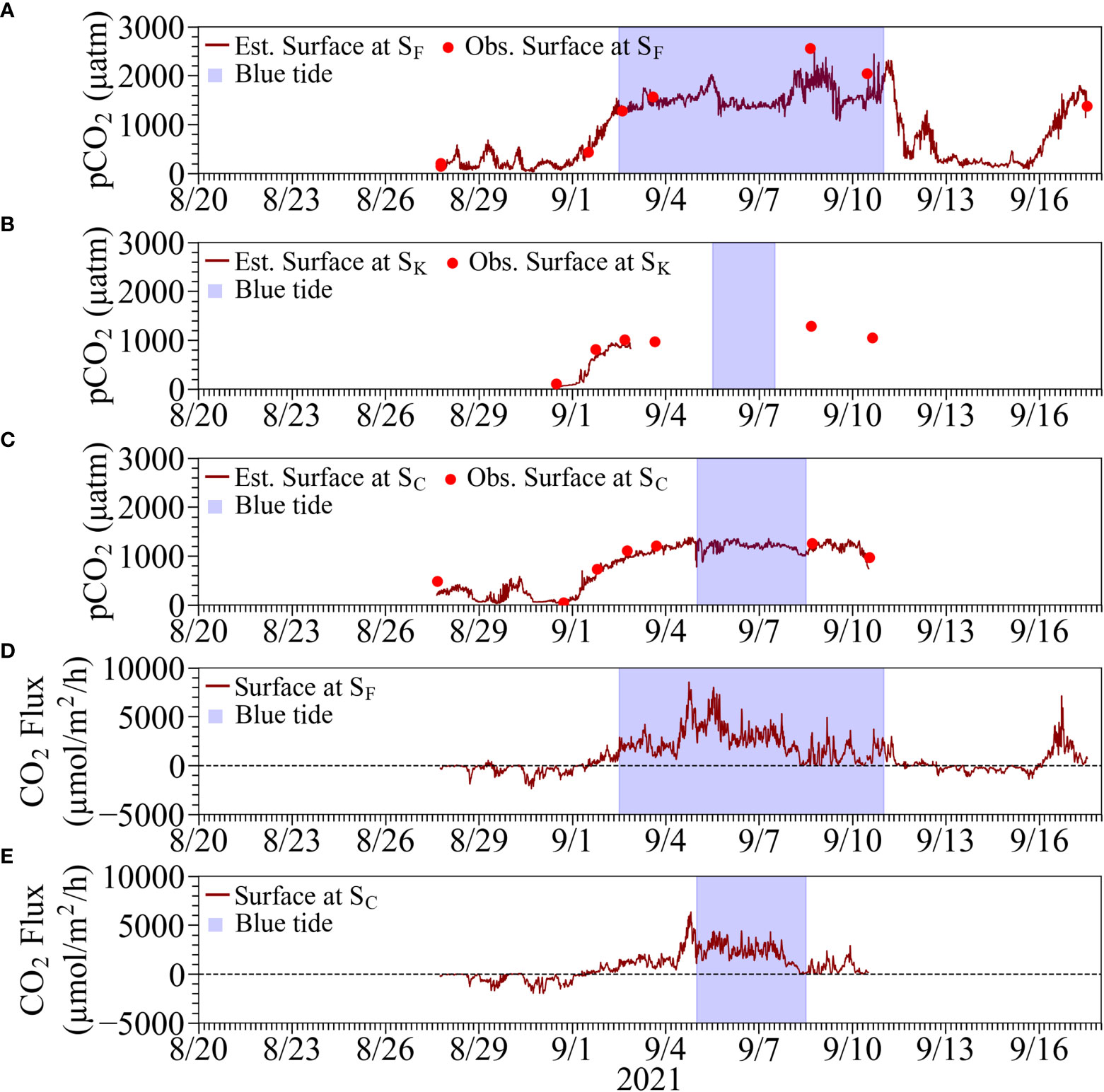
Figure 8 Top three panels are comparisons of estimated continuous pCO₂ from the corrected continuous pH and calculated pCO₂ from the measurements of the corresponding water samples using ATT-05 at (A) Stn. S_F, (B) Stn. S_K, and (C) S_C. Bottom two panels are estimated CO₂ flux at the sea surface (positive value denotes emission) at (D) Stn. S_F and (E) S_C. Results at Stn. S_K were omitted because of the considerable suspension of measurements. The blue tide durations are denoted by hatched boxes in blue.

FIGURE 9

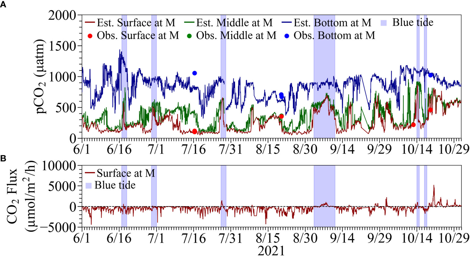
Figure 9 (A) Comparisons of estimated continuous pCO₂ from the corrected continuous pH and calculated pCO₂ from the measurements of the corresponding water samples using ATT-05 at Stn. M. (B) Estimated CO₂ flux at the sea surface (positive values denote emission) at Stn. M. The blue tide durations are denoted by hatched boxes in blue.

Continuous estimates of CO₂ fluxes at Stns. S_F and S_C showed absorption and emission trends before and after noon on September 1, respectively, due to the upwelling and subsequent blue tide (see Figures 8D, E). The mean CO₂ fluxes during the absorption (normal) period were estimated to be −413 µmol m^-2 h^-1 and −491 µmol m^-2 h^-1 at Stns. S_F and S_C, respectively. The mean CO₂ fluxes during the emission (upwelling) period were estimated to be 2153 µmol m^-2 h^-1 and 1540 µmol m^-2 h^-1 at Stns. S_F and S_C, respectively. The absorption trend at Stn. M was similar to those at Stns. S_F and S_C before the onset of the blue tide (see Figure 9B). A slight emission trend was observed during the blue tide, but the degree of emission was estimated to be minor compared to those at Stns. S_F and S_C.

Estimated propagated uncertainties for CO₂ flux were between 1.1 and 17.5 µmol m^-2 h^-1 at Stn. S_F and between 1.1 and 18.2 at Stn. S_C during the absorption period, whereas they were between 11.4 and 60.2 at Stn. S_F and between 12.1 and 34.2 at Stn. S_C during the emission period. These uncertainties were around three percent or less of the typical magnitude of CO₂ flux.

4 Discussion

4.1 Practical TA and pCO₂ estimation for blue tides

We investigated a practical method for continuous estimation of pCO₂ using TA and pH especially targeting surface waters during upwelling of hypoxic and anoxic waters, including blue tides. It is thus important to evaluate the accuracy of estimated TA from salinity and measured pH and their respective contributions to the estimation of pCO₂ in such specific environments.

The measured TA is thought to include the influences of the conservative mixing of freshwater and open ocean water and biogeochemical processes such as photosynthesis, organic matter degradation, and calcification (Jiang et al., 2014). Surface waters in the open ocean and inner bays generally have a high linear correlation between TA and salinity (Lee et al., 2006; Najjar et al., 2020). A high correlation between TA and salinity has also been reported in Tokyo Bay under normal conditions without blue tides (Taguchi et al., 2009). This means that the biogeochemical effect on measured TA is small and almost entirely determined by non-biochemical effects. In this study, a high correlation was observed in surface water, even during the blue tide, strongly influenced by organic matter decomposition (Figure 2). There are, however, some limitations in the estimation of TA, including the slight overestimation and some outliers in the anoxic bottom waters and surface waters with low salinity, as mentioned in subsection 2.4, which should be considered in future research.

The high correlation between TA and salinity, even during the blue tide, is considered the dilution effect of the surface water. Blue tides are caused by the reaction of hydrogen sulfide with oxygen in the surface water to form particulate sulfur during the upwelling of anoxic waters. Therefore, when the water reached the surface, it may have mixed with the original surface water. Figure 6 shows that TA increased rapidly in the anoxic waters at Stn. P_M, the borrow pit, and Figure 2 also shows that TA deviates from the regression line in the bottom layer. This means that biogeochemical effects cannot be neglected in the stagnant anoxic water. However, Figure 7 shows that the measured and estimated TAs of the surface layer were generally consistent even during the blue tide. These results suggest that the biogeochemical effects were minor when the anoxic water reached the surface, due to dilution by the abundant seawater.

The estimated pCO₂ was found to more sensitive to a change in pH than that in TA especially during upwelling events due to the appearance of a significant decrease in pH. The accuracy of observed in situ pH thus plays a key role in obtaining reasonable pCO₂ estimation results. However, the accuracy of self-recording pH sensors for continuous monitoring is considered a challenge. In fact, continuous observations of pH were not suitable for direct use in estimating pCO₂. This is because pH meters moored in the field generally do not meet the accuracy requirements for pCO₂ estimation. It is necessary to correct this by using a higher-accuracy pH meter. We showed that a practical continuous estimation of pCO₂ was possible by calibrating in situ pH meter values using the high-precision pH meter of ATT-05 on water samples. The pCO₂ of the water samples can be estimated by inputting two of the three parameters of pH, TA, and DIC measured by ATT-05 into PyCO2SYS; we confirmed that the calculated pCO₂ values from any two of the three parameters were consistent with each other.

Figure 10 shows the difference in calculated pCO₂ using measured pH and TA for the water samples containing sulfide with and without the consideration of its influence in PyCO2SYS; the pCO₂ is considered overestimated without considering the effect of sulfide (Xu et al., 2017). The difference in pCO₂ was less than 1 µatm at sulfide detection limit of 0.05 mg/L, whereas it was less than 20 µatm at sulfide concentrations of less than 1 mg/L, which were typical in our observation. The time series of pCO₂ calculated by estimated TA and pH did not include the effect of sulfide in the surface layer (Figure 8). However, the concentration of sulfide in the surface layer during the onset of the blue tide was almost zero (Figure 6), suggesting that the error in pCO₂ with and without the consideration of sulfide is small.

FIGURE 10

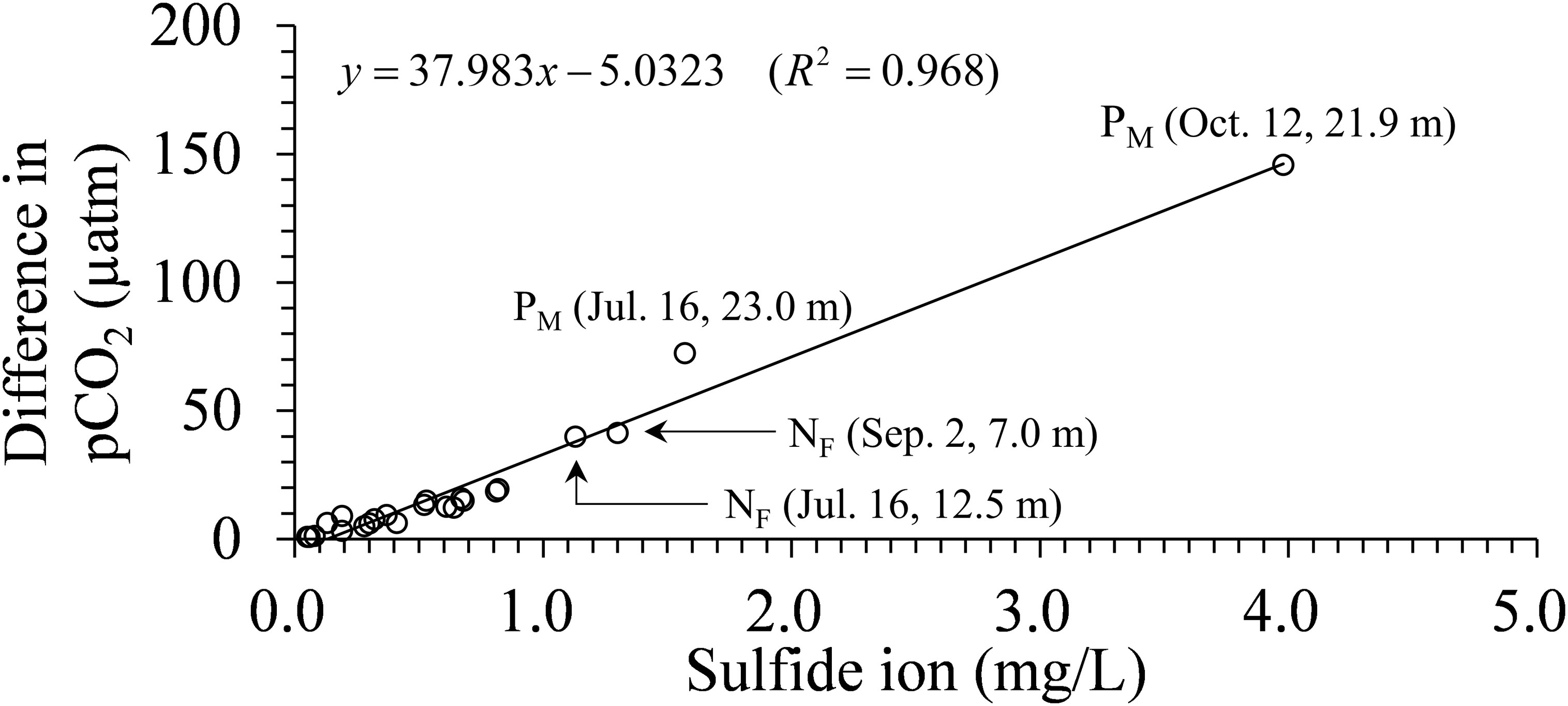
Figure 10 Difference in calculated pCO₂ using measured pH and TA for water samples containing sulfide with and without the consideration of its influence.

Although the estimated results in Figure 8 generally reproduces the variation in pCO₂, a relatively large discrepancy was observed in the surface water at Stn. S_F on September 8 during the blue tide (see Figure 8). This discrepancy was attributed to the significant difference between the pH of the water sample (7.309) and the corrected observed pH (7.487), which may have been caused by the freshwater effect specifically observed in the thin surface layer. Another reason for the underestimation of pCO₂ was that the blue tide in Funabashi was the largest in scale, and the TA estimated from salinity was affected by internal production. However, the increasing pCO₂ process before and during the blue tide and the decreasing process after the end of the blue tide were well reproduced. Therefore, the pCO₂ estimation method developed in this study is considered practical.

However, for the bottom layer at Stn. M on July 16, the number of samples used for the correction was limited, and the pH sensor calibration interval was long, ranging from 2 weeks to 1 month, suggesting that a single regression equation may not have been sufficient. Further study is needed to establish a continuous estimation method of pCO₂ over a long period from seasonal to annual variations, considering the balance between accuracy and cost.

4.2 Relationship between DIC, TA, and estimated pCO₂ for water samples

In the estimation of pCO₂, very high values were found in the bottom layer of the borrow pit (e.g., see Figure 5). Using the dataset of TA, DIC, and pH measured by ATT-05 for water samples, we considered coarbonate dynamics, including pCO₂.

The vertical distribution of pCO₂ at Stn. P_M showed values exceeding 1000 µatm at a depth of 10 m and values exceeding 4000 µatm in the bottom layer (Figure 5). Also, at Stn. N_F3, pCO₂ in the anoxic water always exceeded 1000 atm (Figure 6). It is known that a high TA/DIC ratio results in a low CO₂/DIC ratio tending to a sink for atmospheric CO₂, whereas a low TA/DIC results in a high CO₂ emission tendency. The carbonate buffering capacity is intensified under a larger TA, leading to a smaller decrease in pH with CO₂ dissolution and more capacity for storing pCO₂ (Egleston et al., 2010). The TA/DIC ratios at the surface layers of Stn. P_M and Stn. N_F3 under normal conditions were 1.155 and 1.252, and the corresponding pCO₂ were 242 and 160 µatm, respectively (Figures 5B, 6A–D). This means that the carbonate buffering capacity was strong, and the water was a sink of the atmospheric pCO₂. On the other hand, the TA/DIC ratios of the bottom layers at Stn. P_M and Stn. N_F3 under normal conditions were 0.950 and 0.977, respectively, and pCO₂ exceeded 3000 µatm (Figures 5A, 6A–D). Under normal conditions, the TA/DIC ratio decreased with approaching the bottom, indicating that the area adjacent to the bottom sediment contained high pCO₂ due to the decomposition of organic matter under the stagnant condition.

Figure 11 shows the relationship between DIC and TA for all water samples and calculated pCO₂ using PyCO2SYS considering the influence of sulfide. TA values were higher than DIC for most of the samples. DIC values were higher than TA at the bottom of the navigation channel and borrow pit where sulfides were detected during normal times without blue tide, and at the middle to lower waters where sulfides were detected during the blue tide; pCO₂ values in these waters were higher than 2000 µatm. During the blue tide outbreak, the TA/DIC ratios in the surface layer were 1.029 and 1.034, which were much lower than the values of 1.252 and 1.240 under the normal condition, indicating that the carbonate buffering capacity was weaker (Figures 5D, 6E–H) and thus increasing pCO₂. This is due to the upwelling of anoxic waters affected by organic matter decomposition during the onset of the blue tide. Therefore, during blue tide outbreaks, there was a tendency of high CO₂ emissions.

FIGURE 11

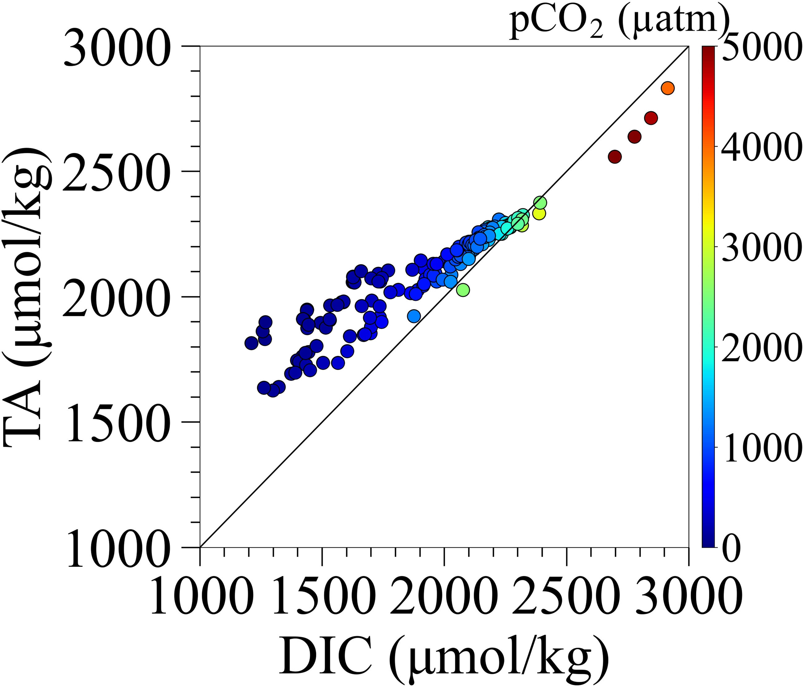
Figure 11 The relationship between measured DIC and TA for water samples and calculated pCO₂ from calc. pH and TA.

Next, we discuss the uniformity of carbonate-chemistry parameters in hypoxic and anoxic waters. First, Figures 5, 6 show that the pH at Stn. P_M was lower than 7.7 in anoxic water, whereas the pH at Stn. N_F3 was higher than that at Stn. P_M, ranging from 7.7 to 8.0. The bottom layer at Stn. P_M on August 20 recorded extremely high pCO₂ with a DIC of 2778 µmol/kg and a TA of 2638 µmol/kg (Figure 5A). On the other hand, on September 16, after the end of the blue tide, pCO₂ rapidly decreased at a depth of 20.54 m (Figure 5D) with a DIC of 2053 µmol/kg and a TA of 2186 µmol/kg in the bottom layer. Even at Stn. N_F3, the pCO₂ under normal conditions on July 16 and August 24 was different. This suggests that carbonate-chemistry parameters in the anoxic waters were not uniform and that the bottom waters in the pit and navigation channel were moved during upwelling.

From Figure 5A, the highest pCO₂ was recorded at a depth of 18.35 m, which contained almost no sulfide. By contrast, changes in sulfide corresponded well with those in pCO₂ during the onset of the blue tide (Figures 6E–H). This suggests that DIC and TA fluctuated in the bottom layer under the influence of organic matter decomposition, but the decomposition pathways contributing to the fluctuations were spatiotemporally different. As a result, carbonate-chemistry parameters in the anoxic water varied widely. Figure 8 also shows that pCO₂ in the surface layer at Stns. S_K and S_C increased even before the onset of the blue tide, indicating that the high pCO₂ values were influenced by organic matter decomposition other than sulfate reduction.

4.3 Impact of blue tide on CO₂ emission

Although surface pCO₂ at the time of upwelling tended to increase at all stations in the bay head, the CO₂ flux suggested that the tendency to release CO₂ to the atmosphere was particularly significant in the period when the blue tide occurred (Figures 8D, E, 9B). These are confirmed by comparing the mean values of CO₂ flux at Stns. S_F and S_C during the emission periods with and without the blue tide as shown in Table 1. The table also shows results using other literature formulas for the piston velocity (Ho et al., 2006; Jiang et al., 2008) not including current speed, which is currently not available. Their results varied, but the absorption and emission trends were consistent among the formulas. Using the formula from Wanninkhof (2014), the CO₂ emissions with blue tide were +2391 µmol m^-2 h^-1 between noon on September 2 and 0:00 a.m. on September 11 at Stn. S_F and +2193 µmol m^-2 h^-1 between 0:00 a.m. on September 5 and noon on September 8 at Stn. S_C, whereas those without blue tide were +809 and +1124 µmol m^-2 h^-1 at Stns. S_F and S_C, respectively. These results suggest that the CO₂ emission was significantly greater with the occurrence of blue tides than without it during the emission period.

TABLE 1

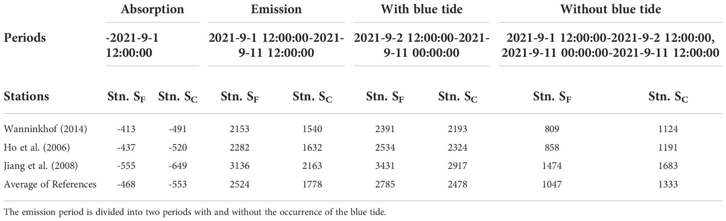
Table 1 Estimated CO₂ fluxes (μmol m^-2 h^-1 at Stns. S_F and S_C during the absorption and emission periods using piston velocities from severalliterature sources.

At Stn. S_F, where higher pCO₂ was observed, turbidity, which is highly correlated with sulfur concentration causing blue tide discoloration, remained higher than at Stn. S_C throughout the observation period (Figure 8). The surface water at Stn. S_F has considered affected by the upwelled waters from the Funabashi navigation channel and off-Makuhari borrow pit. In these waters, the stratification had been intensified during summer with little oxygen supply, whereas the DIC generated by organic matter decomposition accumulated below the pycnocline, which could be a cause of the appearance of extremely high DIC. In addition, the appearance of hydrogen sulfide decreased pH and increased the portion of pCO₂. This suggests that blue tides with higher sulfur concentrations have higher pCO₂ and a stronger tendency to emit to the atmosphere.

Figure 12 shows the time series of pH, TA, and DIC, and calculated pCO₂ using PyCO2SYS at the surface, middle (6–8 m deep), and bottom at Stn. N_F3. The values of these parameters in the surface layer at the time of the blue tide on September 3 were similar to those in the bottom layer on August 24, just before the onset of the blue tide. Therefore, it is considered that the water masses in the bottom layer upwelled while preserving these water quality parameter values. At Stn. N_F6, outside the harbor area and located offshore of Stn. N_F3, the conservative trend was not clearly seen, suggesting that the dilution effect was dominant. In the innermost part of the harbor, the upwelling of bottom anoxic water to the surface with relatively weak dilution is suggested to contribute significantly to the release of CO₂ to the atmosphere.

FIGURE 12

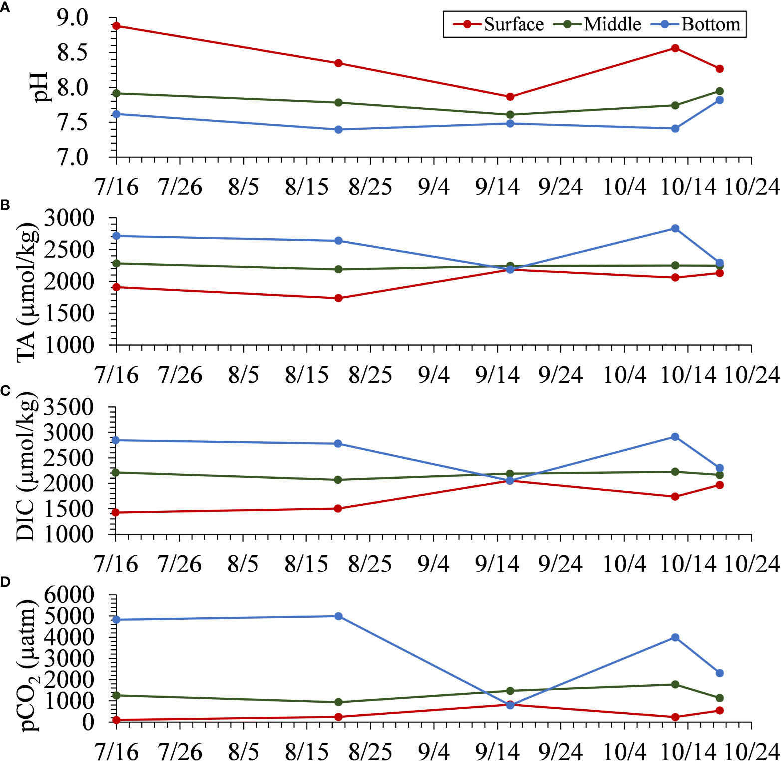
Figure 12 The time series of observed (A) pH, (B) TA, and (C) DIC at the surface, middle, and bottom. (D) The time series of calculated pCO₂ for water samples collected at the surface, middle, and bottom at Stn. N_F3.

Urban bays are expected to be atmospheric CO₂ sinks due to abundant nutrient inputs leading to high primary production and advanced sewage treatment (Kuwae et al., 2016). In particular, Tokyo Bay has been reported to be a year-round atmospheric CO₂ sink because sewage treatment removes labile organic matter more efficiently than nutrient species (Kubo et al., 2017; Tokoro et al., 2021). However, these studies did not adequately account for the effect of the upwelling of anoxic water masses. In this study, we show that pCO₂ was highly elevated in the surface layer during the onset of blue tides and that CO₂ tended to be highly emitted during this period. Because blue tides are localized events that occur at the head of the bay during the summer and autumn, their annual impact on the entire bay may be small. However, it is known that anoxic waters develop in the bay from spring to autumn (Ando et al., 2021), and CO₂ in the hypoxic and anoxic waters may be rapidly released into the atmosphere in autumn when the stratification is destroyed. In the future, it is necessary to accumulate high-resolution spatiotemporal data to clarify the exact annual carbon budget in the bay.

Data availability statement

The raw data supporting the conclusions of this article will be made available by the authors, without undue reservation.

Author contributions

JS (PI) and ME conceived the ideas. ME and YZ collected and analyzed data. ME and JS wrote the manuscript. WN contributed to the discussion. All authors contributed to the article and approved the submitted version.

Funding

This study was funded by Yokohama Port and Airport Technical Research Office, Kanto Regional Development Bureau, Ministry of Land, Infrastructure, Transport and Tourism and JSPS KAKENHI Grant Number JP20H02250.

Acknowledgments

We are grateful to Dr. Toru Endo at Osaka Metropolitan University and Dr. Sosuke Otani at Osaka Metropolitan University College of Technology for their valuable comments in JSPS KAKENHI project on urban blue carbon. Supplementary Material templates can be found in the Frontiers LaTeX folder.

Conflict of interest

The authors declare that the research was conducted in the absence of any commercial or financial relationships that could be construed as a potential conflict of interest.

Publisher’s note

All claims expressed in this article are solely those of the authors and do not necessarily represent those of their affiliated organizations, or those of the publisher, the editors and the reviewers. Any product that may be evaluated in this article, or claim that may be made by its manufacturer, is not guaranteed or endorsed by the publisher.

References

Amunugama M., Sasaki J. (2018). Numerical modeling of long-term biogeochemical processes and its application to sedimentary bed formation in Tokyo Bay. Water 10 (5), 572. doi: 10.3390/w10050572

CrossRef Full Text | Google Scholar

Ando H., Maki H., Kashiwagi N., Ishii Y. (2021). Long-term change in the status of water pollution in Tokyo Bay: Recent trend of increasing bottom-water dissolved oxygen concentrations. J. Oceanogr 77, 843–858. doi: 10.1007/s10872-021-00612-7

CrossRef Full Text | Google Scholar

Aoki K., Shimizu Y., Yamamoto T., Yokouchi K., Kishi K., Akada H., et al. (2022). Estimation of inward nutrient flux from offshore into semi-enclosed sea (Tokyo Bay, Japan) based on in-situ data. Estuarine Coast. Shelf Sci. 274, 107930. doi: 10.1016/j.ecss.2022.107930

CrossRef Full Text | Google Scholar

Benallal M., Moussa H., Lencina-Avila J., Touratier F., Goyet C., Jai M. E., et al. (2017). Satellite-derived CO₂ flux in the surface seawater of the austral ocean south of australia. Int. J. Remote Sens. 38 (6), 1600–1625. doi: 10.1080/01431161.2017.1286054

CrossRef Full Text | Google Scholar

Breitburg D., Levin L. A., Oschlies A., Grégoire M., Chavez F. P., Conley D. J., et al. (2018). Declining oxygen in the global ocean and coastal waters. Science 359 (6371), eaam7240. doi: 10.1126/science.aam7240

PubMed Abstract | CrossRef Full Text | Google Scholar

Breithaupt J. L., Smoak J. M., Smith T. J. III, Sanders C. J., Hoare A. (2012). Organic carbon burial rates inmangrove sediments: Strengthening the global budget. Global Biogeochem Cycles 26, GB3011. doi: 10.1029/2012GB004375

CrossRef Full Text | Google Scholar

Call M., Maher D., Santos I., Ruiz-Halpern S., Mangion P., Sanders C., et al. (2015). Spatial and temporal variability of carbon dioxide and methane fluxes over semi-diurnal and spring–neap–spring timescales in a mangrove creek. Geochimica Cosmochim Acta 150, 211–225. doi: 10.1016/j.gca.2014.11.023

CrossRef Full Text | Google Scholar

Diaz R. J., Rosenberg R. (2008). Spreading dead zones and consequences for marine ecosystems. Science 321 (5891), 926–929. doi: 10.1126/science.1156401

PubMed Abstract | CrossRef Full Text | Google Scholar

Dickson A. G. (1990). Standard potential of the reaction: AgCl(s) + 12H2(g) = Ag(s) + HCl(aq), and and the standard acidity constant of the ion HSO4− in synthetic sea water from 273.15 to 318.15 K. The Journal of Chemical Thermodynamics, 22(2), 113–127. doi: 10.1016/0021-9614(90)90074-Z

CrossRef Full Text | Google Scholar

Dickson A. G., Riley J. P. (1979). The estimation of acid dissociation constants in sea-water media from potentiometric titrations with strong base. II. The dissociation of phosphoric acid. Marine Chemistry 7, 101–109. doi: 10.1016/0304-4203(79)90002-1

CrossRef Full Text | Google Scholar

Dickson A. G., Sabine C. L., Christian J. R. (2007). Guide to best practices for ocean CO₂ measurements. PICES special publication 3. IOCCP report 8 , 191pp. DICKSON2007.

Google Scholar

Duarte C. M., Krause-Jensen D. (2017). Export from seagrass meadows contributes to marine carbon sequestration. Front. Mar. Sci. 4. doi: 10.3389/fmars.2017.00013

CrossRef Full Text | Google Scholar

Egleston E. S., Sabine C. L., Morel F. M. M. (2010). Revelle revisited: Buffer factors that quantify the response of ocean chemistry to changes in dic and alkalinity. Global Biogeochem cycles 24, GB1002. doi: 10.1029/2008GB003407

CrossRef Full Text | Google Scholar

Feely R. A., Sabine C. L., Hernandez-Ayon J. M., Ianson D., Hales B. (2008). Evidence for upwelling of corrosive “acidified” water onto the continental shelf. Science 320, 1490–1492. doi: 10.1126/science.1155676

PubMed Abstract | CrossRef Full Text | Google Scholar

Friedrich T., Oschlies A. (2009). Neural network-based estimates of north atlantic surface pCO₂ from satellite data: A methodological study. J. Geophysical Research: Oceans 114 (C3), 12. doi: 10.1029/2007JC004646

CrossRef Full Text | Google Scholar

Furukawa K. (2015). “Eutrophication in Tokyo Bay,” in Eutrophication and oligotrophication in Japanese estuaries: The present status and future tasks. Ed. Yanagi T. (Dordrecht: Springer Netherlands), 5–37. doi: 10.1007/978-94-017-9915-7

CrossRef Full Text | Google Scholar

Gallardo V., Espinoza C. (2008). The evolution of ocean color. Proc. SPIE - Int. Soc. Optical Eng., 7097. doi: 10.1117/12.794742

CrossRef Full Text | Google Scholar

Gilbert D., Rabalais N., Diaz R., Zhang J. (2010). Evidence for greater oxygen decline rates in the coastal ocean than in the open ocean. Biogeosciences 7, 2283–2296. doi: 10.5194/bg-7-2283-2010

CrossRef Full Text | Google Scholar

Higa H., Sugahara S., Salem S. I., Nakamura Y., Suzuki T. (2020). An estimation method for blue tide distribution in Tokyo Bay based on sulfur concentrations using geostationary ocean color imager (GOCI). Estuarine Coast. Shelf Sci. 235, 106615. doi: 10.1016/j.ecss.2020.106615

CrossRef Full Text | Google Scholar

Ho D. T., Law C. S., Smith M. J., Schlosser P., Harvey M., Hill P. (2006). Measurements of air-sea gas exchange at high wind speeds in the southern ocean: Implications for global parameterizations. Geophysical Res. Lett. 33 (16), 16. doi: 10.1029/2006GL026817

CrossRef Full Text | Google Scholar

Hong B., Xue H., Zhu L., Xu H. (2022). Climatic change of summer wind direction and its impact on hydrodynamic circulation in the pearl river estuary. J. Mar. Sci. Eng. 10 (7). doi: 10.3390/jmse10070842

PubMed Abstract | CrossRef Full Text | Google Scholar

Humphreys M. P., Lewis E. R., Sharp J. D., Pierrot D. (2022). PyCO2SYS v1.8: marine carbonate system calculations in Python. Geoscientific Model. Dev. 15 (1), 15–43. doi: 10.5194/gmd-15-15-2022

CrossRef Full Text | Google Scholar

Jähne B., Heinz G., Dietrich W. (1974). Measurement of the diffusion coefficients of sparingly soluble gases in water. J. Geophysical Research: Oceans 92 (C10), 10767–10776. doi: 10.1029/JC092iC10p10767

CrossRef Full Text | Google Scholar

Jiang L.-Q., Cai W.-J., Wang Y. (2008). A comparative study of carbon dioxide degassing in river- and marine-dominated estuaries. Limnol Oceanogr 53 (6), 2603–2615. doi: 10.4319/lo.2008.53.6.2603

CrossRef Full Text | Google Scholar

Jiang Z.-P., Tyrrell T., Hydes D. J., Dai M., Hartman S. E. (2014). Variability of alkalinity and the alkalinity-salinity relationship in the tropical and subtropical surface ocean. Global Biogeochem Cycles 28 (7), 729–742. doi: 10.1002/2013GB004678

CrossRef Full Text | Google Scholar

Johnson K. S., Jannasch H. W., Coletti L. J., Elrod V. A., Martz T. R., Takeshita Y., et al. (2016). Deep-sea durafet: A pressure tolerant ph sensor designed for global sensor networks. Analytical Chem. 88 (6), 3249–3256. doi: 10.1021/acs.analchem.5b04653

CrossRef Full Text | Google Scholar

Kodama K., Horiguchi T. (2011). Effects of hypoxia on benthic organisms in Tokyo Bay, Japan: A review. Mar. Pollut. Bull. 63, 215–220. doi: 10.1016/j.marpolbul.2011.04.022

PubMed Abstract | CrossRef Full Text | Google Scholar

Krause-Jensen D., Duarte C. M. (2016). Substantial role of macroalgae in marine carbon sequestration. Nat. Geosci 9, 737–742. doi: 10.1038/ngeo2790

CrossRef Full Text | Google Scholar

Kubo A., Maeda Y., Kanda J. (2017). A significant net sink for CO₂ in Tokyo Bay. Sci. Rep. 7, 44355. doi: 10.1038/srep44355

PubMed Abstract | CrossRef Full Text | Google Scholar

Kuwae T., Hori M. (2019). Blue carbon in shallow coastal ecosystems (Singapore: Springer Singapore). doi: 10.1007/978-981-13-1295-3

CrossRef Full Text | Google Scholar

Kuwae T., Kanda J., Kubo A., Nakajima F., Ogawa H., Sohma A., et al. (2016). Blue carbon in human-dominated estuarine and shallow coastal systems. J. Ambio 45, 290–301. doi: 10.1007/s13280-015-0725-x

CrossRef Full Text | Google Scholar

Lee J., Park K.-T., Lim J.-H., Yoon J.-E., Kim I.-N. (2018). Hypoxia in korean coastal waters: A case study of the natural Jinhae Bay and artificial Shihwa Bay. Front. Mar. Sci. 5, 5. doi: 10.3389/fmars.2018.00070

CrossRef Full Text | Google Scholar

Lee K., Kim T.-W., Byrne R. H., Millero F. J., Feely R. A., Liu Y.-M. (2010). The universal ratio of boron to chlorinity for the North Pacific and North Atlantic oceans. Geochimica et Cosmochimica Acta 74, 1801–1811. doi: 10.1016/j.gca.2009.12.027

CrossRef Full Text | Google Scholar

Lee K., Tong L. T., Millero F. J., Sabine C. L., Dickson A. G., Goyet C., et al. (2006). Global relationships of total alkalinity with salinity and temperature in surface waters of the world’s oceans. Geophysical Res. Lett. 33. doi: 10.1029/2006GL027207

CrossRef Full Text | Google Scholar

Lefévre N., Watson A. J., Watson A. R. (2005). A comparison of multiple regression and neural network techniques for mapping in situ pCO₂ data. Tellus B: Chem. Phys. Meteorol 57 (5), 375–384. doi: 10.3402/tellusb.v57i5.16565

CrossRef Full Text | Google Scholar

Liu F., Sasaki J., Chen J., Wang Y. (2022). Numerical assessment of coastal multihazard vulnerability in Tokyo Bay. Natural Hazards 114, 3597–3625. doi: 10.1007/s11069-022-05533-2

CrossRef Full Text | Google Scholar

Lohrenz S. E., Cai W.-J., Chakraborty S., He R., Tian H. (2018). Satellite estimation of coastal pCO₂ and air-sea flux of carbon dioxide in the northern Gulf of Mexico. Remote Sens. Environ. 207, 71–83. doi: 10.1016/j.rse.2017.12.039

CrossRef Full Text | Google Scholar

Ma J., French K. L., Cui X., Bryant D. A., Summons R. E. (2021). Carotenoid biomarkers in namibian shelf sediments: Anoxygenic photosynthesis during sulfide eruptions in the benguela upwelling system. Proc. Natl. Acad. Sci. 118 (29), e2106040118. doi: 10.1073/pnas.2106040118

CrossRef Full Text | Google Scholar

Majkut J. D., Sarmiento J. L., Rodgers K. B. (2014). A growing oceanic carbon uptake: Results from an inversion study of surface pCO₂ data. Global Biogeochem Cycles 28 (4), 335–351. doi: 10.1002/2013GB004585

CrossRef Full Text | Google Scholar

Minghelli-Roman A., Laugier T., Polidori L., Mathieu S., Loubersac L., Gouton P. (2011). Satellite survey of seasonal trophic status and occasional anoxic malaïgue’crises in the Thau lagoon using MERIS images. Int. J. Remote Sens. 32 (4), 909–923. doi: 10.1080/01431160903485794

CrossRef Full Text | Google Scholar

Mohanty S., Raman M., Mitra D., Chauhan P. (2022). Surface pCO₂ variability in two contrasting basins of north indian ocean using satellite data. Deep Sea Res. Part I: Oceanographic Res. Papers 179, 103665. doi: 10.1016/j.dsr.2021.103665

CrossRef Full Text | Google Scholar

Mojica Prieto F. J., Millero F. J. (2002). The values of pK1 + pK2 for the dissociation of carbonic acid in seawater. Geochimica et Cosmochimica Acta 66, 2529–2540. doi: 10.1016/S0016-7037(02)00855-4

CrossRef Full Text | Google Scholar

Moussa H., Benallal M., Goyet C., Lefèvre N. (2016). Satellite-derived CO₂ fugacity in surface seawater of the tropical atlantic ocean using a feedforward neural network. Int. J. Remote Sens. 37 (3), 580–598. doi: 10.1080/01431161.2015.1131872

CrossRef Full Text | Google Scholar

Najjar R. G., Herrmann M., Valle S. M. C. D., Friedman J. R., Friedrichs M. A., Harris L. A., et al. (2020). Alkalinity in tidal tributaries of the Chesapeake Bay. J. Geophysical Research: Oceans 125, e2019JC015597. doi: 10.1029/2019JC015597

CrossRef Full Text | Google Scholar

Nellemann C., Corcoran E., Duarte C. M., Valedes L., De Young C., Fonseca L., et al. (2009). Blue carbon : the role of healthy oceans in binding carbon : a rapid response assessment, UNEP(02)/B659. (Norway: GRID-Arendal).

Google Scholar

Norman M., Parampil S. R., Rutgersson A., Sahlée E. (2013). Influence of coastal upwelling on the air–sea gas exchange of CO₂ in a Baltic Sea basin. Tellus B: Chem. Phys. Meteorol 65, 21831. doi: 10.3402/tellusb.v65i0.21831

CrossRef Full Text | Google Scholar

Orr J. C., Epitalon J.-M., Dickson A. G., Gattuso J.-P. (2018). Routine uncertainty propagation for the marine carbon dioxide system. Mar. Chem. 207, 84–107. doi: 10.1016/j.marchem.2018.10.006

CrossRef Full Text | Google Scholar

Otsubo K., Harashima A., Miyazaki T., Yasuoka Y., Muraoka K. (1991). Field survey and hydraulic study of “aoshio” in Tokyo Bay. Mar. Pollut. Bull. 23, 51–55. doi: 10.1016/0025-326X(91)90649-D

CrossRef Full Text | Google Scholar

Pearson J., Resplandy L., Poupon M. (2022). Coastlines at risk of hypoxia from natural variability in the northern indian ocean. Global Biogeochem Cycles 36 (6), e2021GB007192. doi: 10.1029/2021GB007192

CrossRef Full Text | Google Scholar

Sarma V. V. S. S., Saino T., Sasaoka K., Nojiri Y., Ono T., Ishii M., et al. (2006). Basin-scale pCO₂ distribution using satellite sea surface temperature, Chl a, and climatological salinity in the North Pacific in spring and summer. Global Biogeochem Cycles 20 (3), 13. doi: 10.1029/2005GB002594

CrossRef Full Text | Google Scholar

Sasaki J., Ito K., Suzuki T., Wiyono R. U. A., Oda Y., Takayama Y., et al. (2012). Behavior of the 2011 tohoku earthquake tsunami and resultant damage in Tokyo Bay. Coast. Eng. J. 54, 1250012. doi: 10.1142/S057856341250012X

CrossRef Full Text | Google Scholar

Sasaki J., Kanayama S., Nakase K., Kino S. (2009a). Effective application of a mechanical circulator for reducing hypoxia in an estuarine trench. Coast. Eng. J. 51, 309–339. doi: 10.1142/S0578563409002053

CrossRef Full Text | Google Scholar

Sasaki J., Kawamoto S., Yoshimoto Y., Ishii M., Kakino J. (2009b). Evaluation of the amount of hydrogen sulfide in a dredged trench of Tokyo Bay. J. Coast. Res. SI56, 890–894.

Google Scholar

Schunck H., Lavik G., Desai D. K., Großkopf T., Kalvelage T., Löscher C. R., et al. (2013). Giant hydrogen sulfide plume in the oxygen minimum zone off Peru supports chemolithoautotrophy. PloS One 8 (8), 1–18. doi: 10.1371/journal.pone.0068661

CrossRef Full Text | Google Scholar

Signorini S. R., Mannino A., Najjar R. G. Jr., Friedrichs M. A. M., Cai W.-J., Salisbury J., et al. (2013). Surface ocean pCO₂ seasonality and sea-air CO₂ flux estimates for the North American east coast. J. Geophysical Research: Oceans 118 (10), 5439–5460. doi: 10.1002/jgrc.20369

CrossRef Full Text | Google Scholar

Stephens M. P., Samuels G., Olson D. B., Fine R. A., Takahashi T. (1995). Sea-Air flux of CO₂ in the North Pacific using shipboard and satellite data. J. Geophysical Research: Oceans 100 (C7), 13571–13583. doi: 10.1029/95JC00901

CrossRef Full Text | Google Scholar

Taguchi F., Fujiwara T., Yamada Y., Fujita K., Sugiyama M. (2009). Alkalinity in coastal seas around Japan. Bull. Coast. Oceanogr 47 (1), 71–75. doi: 10.32142/engankaiyo.47.1_71

CrossRef Full Text | Google Scholar

Testa J. M., Clark J. B., Dennison W. C., Donovan E. C., Fisher A. W., Ni W., et al. (2017). Ecological forecasting and the science of hypoxia in Chesapeake Bay. BioScience 67 (7), 614–626. doi: 10.1093/biosci/bix048

CrossRef Full Text | Google Scholar

Tokoro T., Hosokawa S., Miyoshi E., Tada K., Watanabe K., Montani S., et al. (2014). Net uptake of atmospheric CO₂ by coastal submerged aquatic vegetation. Global Change Biol. 20 (6), 1873–1884. doi: 10.1111/gcb.12543

CrossRef Full Text | Google Scholar

Tokoro T., Nakaoka S., Takao S., Kuwae T., Kubo A., Endo T., et al. (2021). Contribution of biological effects to carbonate-system variations and the air–water CO₂ flux in urbanized bays in japan. J. Geophysical Research: Oceans 126 (6), e2020JC016974. doi: 10.1029/2020JC016974

CrossRef Full Text | Google Scholar

Tokoro T., Watanabe A., Kayanne H., Nadaoka K., Tamura H., Nozaki K., et al. (2007). Measurement of air–water CO₂ transfer at four coastal sites using a chamber method. J. Mar. Syst. 66 (1), 140–149. doi: 10.1016/j.jmarsys.2006.04.010

CrossRef Full Text | Google Scholar

Tomita A., Nakura Y., Ishikawa T. (2016). New direction for environmental water management. Mar. Pollut. Bull. 102, 323–328. doi: 10.1016/j.marpolbul.2015.07.068

PubMed Abstract | CrossRef Full Text | Google Scholar

Vaquer-Sunyer R., Duarte C. M. (2008). Thresholds of hypoxia for marine biodiversity. Proc. Natl. Acad. Sci. 105 (40), 15452–15457. doi: 10.1073/pnas.0803833105

CrossRef Full Text | Google Scholar

Wang K., Nakamura Y., Sasaki J., Inoue T., Higa H., Suzuki T., et al. (2022). An effective process-based modeling approach for predicting hypoxia and blue tide in Tokyo Bay. Coast. Eng. J. 64 (3), 458–476. doi: 10.1080/21664250.2022.2119011

CrossRef Full Text | Google Scholar

Wanninkhof R. (1992). Relationship between wind speed and gas exchange over the ocean. J. Geophysical Research: Oceans 97, 7373–7382. doi: 10.1029/92JC00188

CrossRef Full Text | Google Scholar

Wanninkhof R. (2014). Relationship between wind speed and gas exchange over the ocean revisited. Limnol Oceanogr: Methods 12 (6), 351–362. doi: 10.4319/lom.2014.12.351

CrossRef Full Text | Google Scholar

Weiss R. (1974). Carbon dioxide in water and seawater: the solubility of a non-ideal gas. Mar. Chem. 2 (3), 203–215. doi: 10.1016/0304-4203(74)90015-2

CrossRef Full Text | Google Scholar

Williams N. L., Juranek L. W., Feely R. A., Johnson K. S., Sarmiento J. L., Talley L. D., et al. (2017). Calculating surface ocean pCO₂ from biogeochemical argo floats equipped with pH: An uncertainty analysis. Global Biogeochem Cycles 31 (3), 591–604. doi: 10.1002/2016GB005541

CrossRef Full Text | Google Scholar

Williams N. L., Juranek L. W., Johnson K. S., Feely R. A., Riser S. C., Talley L. D., et al. (2016). Empirical algorithms to estimate water column pH in the southern ocean. Geophysical Res. Lett. 43 (7), 3415–3422. doi: 10.1002/2016GL068539

CrossRef Full Text | Google Scholar

Xu Y.-Y., Pierrot D., Cai W.-J. (2017). Ocean carbonate system computation for anoxic waters using an updated CO2SYS program. Mar. Chem. 195, 90–93. doi: 10.1016/j.marchem.2017.07.002

CrossRef Full Text | Google Scholar

Yamamoto T. (2003). The seto inland Sea —- eutrophic or oligotrophic? Mar. Pollut. Bull. 47, 37–42. doi: 10.1016/S0025-326X(02)00416-2

PubMed Abstract | CrossRef Full Text | Google Scholar

Zemmelink H. J., Slagter H. A., van Slooten C., Snoek J., Heusinkveld B., Elbers J., et al. (2009). Primary production and eddy correlation measurements of CO₂ exchange over an intertidal estuary. Geophysical Res. Lett. 36 (19), 5. doi: 10.1029/2009GL039285

CrossRef Full Text | Google Scholar