Investigating beaked whale’s regional habitat division and local density trends near the Deepwater Horizon oil spill site through acoustics

Pre-spill and post-spill passive acoustic data collected by multiple fixed acoustic sensors monitoring about 2400 km² area to the west of the Deepwater Horizon oil spill in the northern Gulf of Mexico (GoM) were analyzed to understand long term local density trends and habitat use by different species of beaked whales. The data were collected in the Mississippi Valley/Canyon area between 2007 and 2017. A multistage algorithm based on unsupervised machine learning was developed to detect and classify different species of beaked whales and to derive species- and site-specific densities in different years before and after the oil spill. The results suggest that beaked whales continued to occupy and feed in these areas following the Deepwater Horizon oil spill thus raising concerns about (1) potential long-term effects of the spill on these species and (2) the habitat conditions after the spill. The average estimated local density of Cuvier’s beaked whales at the closest site, about 16 km away from the spill location showed statistically significant increase from July 2007 to September 2010, and then from September 2010 to 2015. This is the first acoustic study showing that Gervais’ beaked whales are predominantly present at the shallow site and that Cuvier’s species dominate at two deeper sites, supporting the habitat division (ecological niche) hypothesis. The findings call for continuing high-spatial-resolution long-term observations to fully characterize baseline beaked whale population and habitat use, to understand the causes of regional migrations, and to monitor the long-term impact of the spill.

1 Introduction

Beaked whales are elusive deep-diving marine mammals. They are known to be the most extreme divers among air-breathing marine mammals, capable of diving down to depths of 3000 m and remaining underwater for over 2 hours during a single dive (Tyack et al., 2006; Schorr et al., 2014). With their low profile above water and with the majority of the day spent diving, visual observations are challenging, with the likelihood of sighting animals most favorable in sea states lower than 3 (Tyack et al., 2006; Robbins et al, 2022). Thus, the species’ densities and habitat use information are limited and difficult to obtain via traditional visual transect surveys. Four species of beaked whales have been identified visually and through strandings in the northern Gulf of Mexico (GoM): Cuvier’s (Ziphius cavirostris) and three species of Mesoplodon (Gervais, M. europaeus Blainville’s, M. densirostris (Johnson et al., 2006); and Sowerby’s, M. bidens (Würsig, 2017; NMFS, 2021; NOAA, 2022). The GoM stock status is defined as unknown by NOAA, with the best visual abundance estimates being 18 for Cuvier’s beaked whales and 98 for the Mesoplodon species combined. (NOAA, 2022). However, the most recent synthesis of available transect survey data into the habitat-based cetacean density model estimated the mean abundance of beaked whales in the GoM as 2019 individuals with the associated coefficient of variation (CV) of 0.16 and the model-predicted mean GoM densities range from 0.5 to 6 individuals per 100 km², with the highest density near 1000 m isobaths (Roberts et al., 2016). Such discrepancies in the published stock abundance estimates indicate a need for systematic, high temporal- and spatial-resolution data collection and the use of complementary methodologies to provide higher accuracy estimates of the beaked whale population in the GoM.

Due to unique echolocation foraging clicks produced by each species of beaked whale, Passive Acoustic Monitoring (PAM) techniques offer a robust and cost-efficient solution for studying these stocks (Marques et al., 2009; Marques et al., 2013; Küsel et al., 2011; Hildebrand et al., 2015; Moretti et al., 2010). The first acoustic recordings of the northern GoM beaked whale species were made in July 2007 by the Littoral Acoustic Demonstration Center-Gulf of Ecological Monitoring and Modeling (LADC-GEMM) during a two-week visual-PAM survey in the Mississippi Canyon/Valley area in the vicinity of the future site of the Deepwater Horizon (DWH) oil spill (April 20, 2010 – September 19, 2010). Both Cuvier’s and Mesoplodon’s species of beaked whales were visually observed and later identified in acoustic recordings. That was the only pre-spill acoustic baseline dataset of the regional presence of beaked whale species. The beaked whale habitat was largely impacted by DWH oil spill (Love et al., 2015; McNutt et al., 2012; Takeshita et al., 2017). Starting in 2010, acoustic monitoring projects were conducted in the region and across the GoM. to understand the long-term impact of the spill on regional populations of marine mammals (Ackleh et al., 2012; Hildebrand et al., 2015; Dyer et al., 2015; Hildebrand et al., 2019; Sidorovskaia, 2019; Guilment et al., 2020; Li et al., 2021). Unlike other datasets providing coarse spatial resolution observations across large regions of the GoM, the LADC-GEMM data collection methodology focused on habitat use on the regional scale (Mississippi Canyon (MC) area). The locations were in the proximity of another long-term acoustic survey (Hildebrand et al., 2015), but the Scripps system was placed in shallower water and was recording in a single location in the region (Figure 1), whereas the study discussed here had three sites (referred for brevity as Northern, Southern, and Western). The objective of this paper is to analyze acoustic data collected by the LADC-GEMM consortium before and after the spill, using acoustic activity as an indicator of changes in habitat use and local density of beaked whales.

FIGURE 1

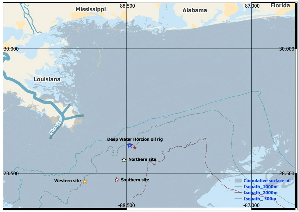
Figure 1 EARS buoys deployment sites (Northern, Southern, and Western). 500, 1000, 2000 m isobaths are shown. The distance between the Northern and Western sites is 55 km, the distance between the Southern and Western sites is 35 km, and the distance between the Northern and Southern sites is 27 km. The red star symbol represents the DWH spill site (28°C44.65’N, 88°C21.10’W). Dark-blue overlay represents the extent of imaged surface oil plume. The blue star symbol represents the deployment site of the SCRIPPS HARP system (Hildebrand et al., 2015).

2 Materials and methods

2.1 Experiment and dataset collection

The LADC-GEMM consortium began collecting acoustic data in 2001 in order to study potential anthropogenic impacts on GoM marine mammals, with emphasis on sperm and beaked whales and deepwater dolphin species. The results presented in this paper are based on data collected near the DWH spill site, as part of the overall data collection effort. The data used for this study were collected in 2007, 2010, 2015 and 2017 at three sites, henceforth referred to as Northern (N), Southern (S), and Western (W) sites (Figure 1) that were about 16, 40 and 80 km away from the DWH spill site, respectively. As a comparison, the location of a PAM unit deployed by the Scripps HARP system (Hildebrand et al., 2015) is also shown in Figure 1. The N and S sites are 1500 m deep and were originally chosen in 2007 because of the high concentration of beaked whales from the NOAA’s National Marine Fisheries Service visual surveys (Waring et al., 2011). The W site is 1000 m deep and is densely populated by sperm whales (Waring et al., 2011; Ackleh et al., 2012).

Each site had one or several bottom-anchored deepwater PAM moorings. All short-term, approximately two-weeks in duration (2007 and 2010), and long-term, over four-months in duration (2015 and 2017), data were collected by the Environmental Acoustic Recording System (EARS) buoys which are bottom-anchored continuous autonomous recorders sampling at 192 kHz (Ioup et al., 2016). Single or paired hydrophones (1m apart) were positioned about 500 m above the bottom at the N and S sites and 250 m above the bottom at the W site. The hydrophone depths were chosen based on propagation modeling results used to design the 2007 sensor placement. The hydrophone depths were targeting the sperm and beaked whale’s foraging depths to increase the probability of detection of their directional echolocation clicks and to provide sufficient temporal separation between direct and bottom reflected signals for near-bottom sound sources. This allows reflected arrivals to be excluded from counting in abundance estimates (Sidorovskaia et al., 2004). The hydrophone depths were kept the same across different deployments. Details of each year and site deployment for the data used in this study are presented in Table 1.

TABLE 1

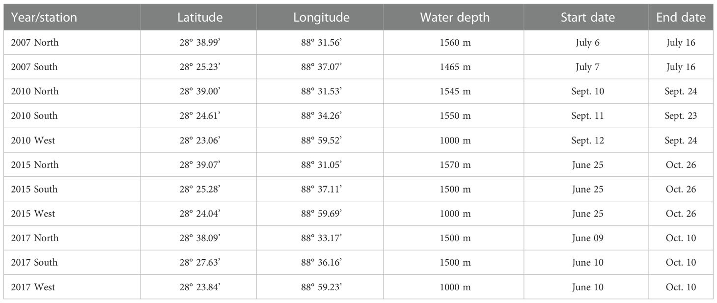
Table 1 Geographic locations of EARS buoy moorings and the start/deployment and end/retrieval dates.

The hydrophones were calibrated at the manufacturing facilities (Sensor Technologies LTD). The hydrophone sensitivity was about -201 dB re 1V/µPa with a flat frequency response curve across the frequency band of 200 Hz-70 kHz. The gain was set to 39.5 dB. The analog-to-digital converter was 16-bit with a full voltage range of 4V. The system calibration values were used to convert digitized data to pressure (in microPascals, µPa). The system was fitted with a high-pass filter with a corner frequency of 200 Hz to reduce signal clipping and contamination of the high-frequency spectrum due to very high industrial activity in the area.

2.2 Density estimation of beaked whales

The local density estimates, based on the detection and counting of acoustic cues at a fixed hydrophone, were obtained following Marques et al., 2009:

$\begin{array}{ll}\widehat{\mathit{D}}=\frac{{\mathit{n}}_{\mathbf{c}}\left(1-\widehat{c}\right)}{\pi w^2{\widehat{P}}_{d}T\widehat{r},}& (1)\end{array}$

where n_c is the number of detected cues over a time period, T , $\widehat{c}$ denotes the estimated proportion of false positive detections, and w is the maximum cue detection range for a hydrophone. ${\widehat{P}}_d$ is the estimated average probability of detecting a cue given that the cue is produced within the detection radius, and $\widehat{r}$ is the estimated cue production rate (e.g., number of clicks per minute) per individual beaked whale.

2.2.1 Number of detected and classified beaked whale clicks

To detect and classify the acoustic signals of beaked whales, we developed the multistage detection and classification algorithm that was described in detail by Li et al., 2020. As the first stage, a band-energy detector was used to compare energy against baseline levels in the band of interest: low band (3-20 kHz), medium band (25-55 kHz), and high band (60-90 kHz). A potential beaked whale click was flagged when the energy was above the background level by a user-specified threshold only in the medium frequency band. The threshold was determined by computing the mean and standard deviation of the sum of the squared spectral amplitude for a given time series over 10-min time intervals. A 10 standard deviation value above the 10-min mean was chosen as the threshold in this study. The threshold can change every 10-min depending on the acoustic background variability. This approach allowed the initial discrimination of beaked whale clicks from sperm whale calls (where energy would be above the threshold only in the low band) and the majority of dolphin clicks (where energy would be above the band-specific thresholds in all three bands). The stated dynamic threshold was chosen based on an experienced operator’s manual analysis to exclude reflected clicks and prevent considerable overestimation of the detected clicks. The second-stage detector performed a sequential multi-attribute analysis of the spectra of the detection events flagged at the first stage. The attribute sequence included a peak frequency, bandwidth, click temporal duration, and sweep slope intervals (Li et al., 2020). The reduced set of detection events was then passed to the third stage detector that performed unsupervised clustering (Li et al., 2020) to classify the different species of beaked whales. The third stage detector output provided the detections of beaked whale species. Three different species of beaked whales were automatically identified at all three sites: Cuvier’s, Gervais’, and BWG (Beaked Whale of the Gulf, following the nomenclature proposed by Hildebrand et al., 2015).

2.2.2 False-alarm estimation

All final species-specific detections were manually examined through reviewing raw signal temporal and spectral signatures to remove all false clicks and to correct misclassified beaked whale species. Due to low rates of false positive detections and species misclassifications after the described above three-step algorithm, all false detections were removed. In the subsequent analysis, the estimated proportion of false positive detections in Eq. (1) was set to zero, $\widehat{c}$=0.

2.2.3 Probability of detection

The probability of detection was estimated by using the methodology discussed in Küsel et al., 2011, and the terminology/notations aligned with the international standards (ISO, 2017; Ainslie et al., 2022). The method consists of two parts. The first part is to simulate the signal-to-noise power ratio (R_sn ) of a received beaked whale click following the passive sonar equation technique:

$\begin{array}{ll}\mathbf{10}\mathit{l}\mathit{o}{\mathit{g}}_{\mathit{10}}{\mathit{R}}_{\mathit{s}\mathit{n}}\left(\mathit{d}\mathit{B}\right)={\mathit{L}}_{\mathit{S}}-{\mathit{L}}_{\mathit{D}\mathit{L}}\left(\mathit{\theta }\right)-{\mathit{N}}_{\mathit{P}\mathit{L}}-{\mathit{L}}_{\mathit{p},\mathit{n}}+\mathit{\Delta }{\mathit{L}}_{\mathit{P}\mathit{G}}& \text{, (2)}\end{array}$

where L_S is the source level (SL, in dB re 1µPa²m²), L_DL is the click directivity (loss which is corresponding to the off-axis attenuation of the source level at a given angle, θ, from the animal’s acoustic axis), N_PL  is the propagation loss, L_p,n is the sound pressure level of noise, and ΔL_PG is the processing gain (set to zero for simulations). Each parameter in Eq (2) was characterized by a relevant statistical distribution from previously published literature and was used in the Monte Carlo algorithm. To estimate R_sn, the whale location and orientation with respect to a receiver is also simulated following Küsel et al., 2011.

The source levels, L_S,   of 225 dB re 1 μPa²m² and 220 dB re 1 μPa²m² for Cuvier’s and Gervais’ beaked whales (Hildebrand et al., 2015), respectively, were used. The off-axis attenuation of source level/click directionality (source level direction dependence) was taken into account by using the flat circular piston model (Au, 1993; Zimmer et al., 2005; Au and Hastings, 2008; Guilment et al., 2020):

$\begin{array}{ll}\mathit{S}\left(\mathit{\theta }\mathit{,} \mathit{f}\right)=\mathit{2}{\mathit{S}}_{\mathbf{0}}\frac{{\mathit{J}}_{\mathbf{1}}\left(\mathit{x}\right)}{\mathit{x}},& (3)\end{array}$

$\begin{array}{ll}\mathit{x}=\frac{\mathit{2}\mathit{\pi }\mathit{f}\mathit{a}\mathit{s}\mathit{i}\mathit{n}\left(\mathbf{\theta }\right)}{\mathit{c}},& (4)\end{array}$

where S represents the angular-dependent power spectral density of the source, S₀ is the reference spectral density, J₁ is the Bessel function of the first kind, f is the given frequency, a is the model piston radius, θ is the angle between the source acoustic axis (corresponding to the maximum emitted level direction) and the direction towards a receiver, and c is the reference mean sound speed in the regional waters. The reference sound speed of 1500 m/s was chosen to be used in the piston model.

The piston model was used to calculate the broadband beam pattern, which could be estimated by integrating S(θ, f) with respect to the frequency. The broadband beam pattern was given by (Zimmer et al., 2005):

$\begin{array}{ll}\mathit{B}\left(\mathbf{\theta }\right)=\frac{{\int }_{-\infty }^{\infty }\mathit{S}\left(\mathit{\theta }\mathit{,} \mathit{f}\right){\mathit{W}}^{\mathbf{2}}\left(\mathit{f}\right)\mathit{d}\mathit{f}}{{\int }_{-\infty }^{\infty }{\mathit{W}}^{\mathit{2}}\left(\mathit{f}\right)\mathit{d}\mathit{f}},& (5)\end{array}$

where W(f) was the Gaussian weighting function. It was given by:

$\begin{array}{ll}\mathit{W}\left(\mathit{f}\right)=\mathit{e}\mathit{x}\mathit{p}\left\{\mathbf{-}\frac{\mathbf{1}}{\mathbf{2}}{\left(\frac{\mathit{f}\mathit{-}{\mathit{f}}_{\mathit{0}}}{\mathit{b}}\right)}^2\right\},& (6)\end{array}$

where f₀ and b were the center frequency and rms bandwidth, respectively.

Then, the off-axis attenuation of source level was finally given by (Zimmer et al., 2005):

$\begin{array}{ll}{\mathit{L}}_{\mathit{D}\mathit{L}}=\mathbf{10}\mathit{l}\mathit{o}\mathit{g}\mathit{B}\left(\mathit{\theta }\right),& \text{, (7)}\end{array}$

Figure 2 shows the attenuation of the source level as a function of off-axis angle for Cuvier’s and Gervais’ beaked whales. Note that the source level at off-axis angles greater than 90° (θ∈[90°,180°] ) is set to the minimum value (at θ=90°) when a whale is echolocating away from the hydrophone. (Zimmer et al., 2008).

FIGURE 2

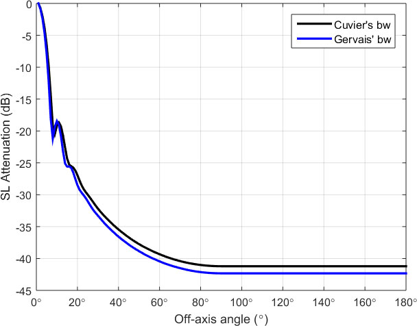
Figure 2 Attenuation of source levels as a function of off-axis angle for Cuvier’s and Gervais’ beaked whales, estimated by using a piston model with radius of 16 cm.

Table 2 summarizes the parameters used in this study for the beaked whale directivity loss calculations.

TABLE 2

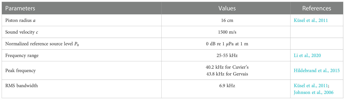
Table 2 Parameters for directivity model.

The propagation loss was modeled by taking into account spherical spreading and absorption loss (Urick, 1983):

$\begin{array}{ll}{\mathit{N}}_{\mathit{P}\mathit{L}}\left(\mathit{r}\right)=\mathbf{20}\mathit{log}\left(\mathit{r}\right)+{\mathit{\alpha }}_{\mathit{f}}\frac{\mathit{r}}{\mathbf{1000}} ,& (8)\end{array}$

where r was the distance between a hypothetical source (whale) placement and a receiver and α_f was the frequency-dependent absorption coefficient expressed in dB/km. The values of 10.05 dB/km (corresponding to a frequency of 40.2 kHz) and 11.30 dB/km (corresponding to a frequency of 43.8 kHz) were chosen for Cuvier’s and Gervais’ beaked whales for the propagation loss calculation (Hildebrand et al., 2015).

The ambient noise levels were estimated by calculating the ambient noise power spectral density (PSD) of the data over the frequency band between 25 and 55 kHz within a representative 8-min period on each hydrophone for each survey year. The 8-min period was chosen to be the same as the period with manually annotated clicks. The ambient noise power was measured by computing the power spectral density for each signal segment between consecutive clicks (considered to be only noise) individually, and then the average of ambient noise level was given by calculating the mean of these segments. The ambient noise level, L_{p, n}, was given by:

$\begin{array}{ll}{\mathit{L}}_{\mathit{p}\mathit{,}\mathit{n}}=\mathit{10}\mathit{l}\mathit{o}\mathit{g}\left(\underset{{\mathbf{f}}_{\mathbf{l}}}{\overset{{\mathbf{f}}_{\mathbf{h}}}{\int }}\mathit{P}\mathit{S}\mathit{D}\mathit{d}\mathit{f}\right),& (9)\end{array}$

where f_l (=25 kHz) and f_h (=55kHz) were lower and upper frequency, respectively, PSD represents the power spectral density of the ambient noise when no clicks are present (annotated).

Once the parameters in the sonar equation were introduced, they were fed into the Monte Carlo Model (MCM), which samples parameter distribution space, including an animal’s position and orientation, and simulates a click. For example, whale’s position in a horizontal plane was simulated by using a uniform distribution within a radius of 10 km under the assumption that whales are randomly distributed in the horizontal plane around a deep hydrophone (Küsel et al., 2011). A click produced larger than 10 km from the hydrophone was assumed to be undetectable. In this study, 100,000 clicks were randomly simulated using hypothetical whale placement within a radius of 10 km and acoustic axis orientation. 500 iterations of the simulations were conducted to incorporate the parameter uncertainty into MCM. The depth positions were divided into three dive phases. The ascent, descent and foraging phases with click proportion, mean depth and pitch distribution used in the simulation are presented in Table 3.

TABLE 3

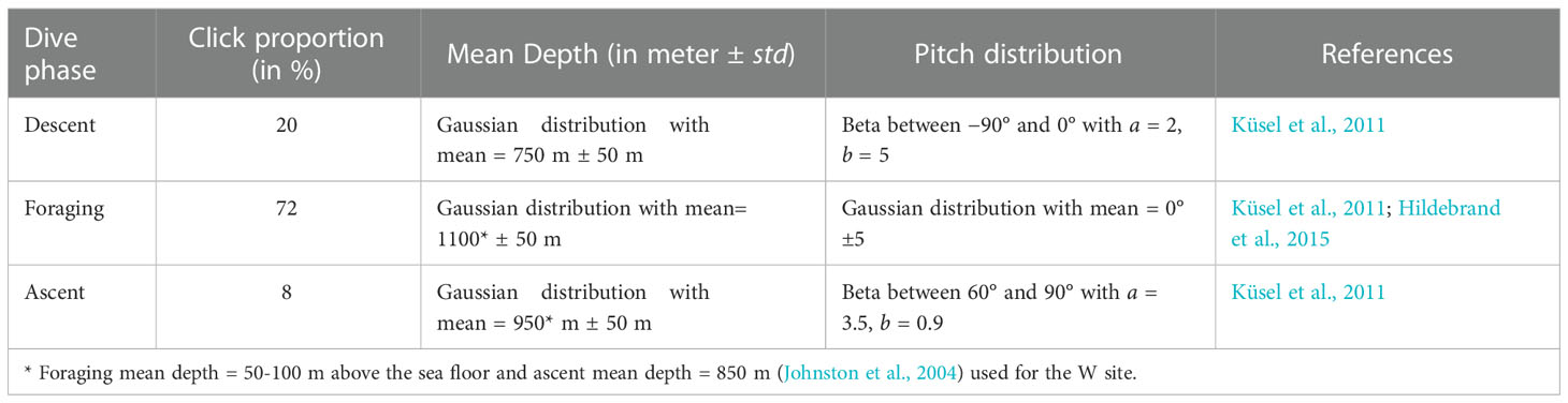
Table 3 Parameters to generate animal locations and orientations for the Monte Carlo simulation.

The distribution of pitch angle of a whale was modelled by a beta distribution for the descending and ascending phases, and pitch angle for the foraging phase was modelled by a Gaussian distribution with mean of 0° and standard deviation of 5° (Hildebrand et al., 2015) from the horizontal plane to allow a whale echolocating in a horizontal direction to be oriented up or down with a small angle.

For each hydrophone location, the representative 8-min data samples having Cuvier’s and Gervais’ beaked whale clicks for each survey year were randomly selected based on the detection datasets to characterize the detector performance at different SNRs (between 0 and 25 dB). A total of 22 8-min data samples were analyzed for the selected datasets. An analyst marked each whale click in the 8-min segment based on the manual analysis of the short-term spectrograms as ground truth. Each MCM generated click with a known range to a receiver was assigned the probability of detection based on the detector performance curve (Küsel et al., 2011). Due to the correlation of the detection range and the SNR distribution, the probability of detection as a function of range was obtained by converting the probability of detection versus SNR into the probability of detection versus the range (Küsel et al., 2011). The estimated probability-of-detection curves vs range for beaked whales are presented in the results section. The average probability of detection was then obtained by integrating the product of probability-of-detection function and the distribution of horizontal object distances, h(y) , which was given by h(y)=2y/w² (where y referred to the horizontal distance, y∈[1, w] , Marques et al., 2009).

2.2.4 Click production rate

The click production rate, which gives the average number of clicks produced per unit time per beaked whale, is a key parameter for the density estimation from passive acoustic data. Several studies have proposed methods to estimate the inter-click interval (ICI) of Cuvier’s beaked whales and Gervais’ beaked whales (Baumann-Pickering et al., 2013; Frantzis et al., 2002; Hildebrand et al., 2015; Warren et al., 2017). An intuitive estimation for the number of cues produced by an individual per unit time can be roughly calculated by simply taking the inverse of the mean ICI. However, the echolocation clicks detectable are only produced during the deep part of a dive (>500m) and are interspersed with occasional buzzes and short pauses (Zimmer et al., 2005; Tyack et al., 2006). Thus, using the inverse of the mean ICIs as an estimate of the click production rate will result in overestimated click production rate. In this study, the following formula is used to estimate the click production rate:

$\begin{array}{ll}\widehat{\mathit{r}}=\frac{{\widehat{\mathit{t}}}_{\mathit{v}}\mathit{-}{\widehat{\mathit{t}}}_{\mathit{b}}}{\mathit{F}\mathit{D}\mathit{C}}\mathit{\times }\frac{\mathbf{1}}{\mathit{I}\mathit{C}\mathit{I}}& \text{, (10)}\end{array}$

where FDC= 121 min (s.d. = 36 min) represents the time of a Full deep Dive foraging Cycle (FDC) for Ziphius (Tyack et al., 2006), which is the interval between the end of one deep dive and the end of the next deep dive, ${\widehat{t}}_v$ represents the vocal duration of the beaked whales as time spent primarily for foraging (Tyack et al., 2006), and ${\widehat{t}}_b$ represents the time spent for producing buzzes. The vocal duration can be approximately calculated as aerobic dive limit (ADL) by dividing total body oxygen stores by diving metabolic rate (Quick et al., 2020). The vocal duration has been reported for Cuvier’s beaked whale as 33 minutes and for Blainville’s beaked whale as 26 minutes per dive (Tyack et al., 2006). The buzz producing time ${\widehat{t}}_b$ can be approximately expressed as the product of the average number of buzzes per dive, N_b , and the average length of each buzz, L_b . The detected buzzes can serve as a proxy for studies on beaked whale habitat use and population health (Jarvis et al., 2022), and in this study, we used N_b and L_b from the reference literature.  N_b is estimated to be 27 per dive for Cuvier’s and 23 for Blainville’s (Johnson et al., 2004) acting as a proxy for Gervais’ beaked whale. L_b was 2.9 s with standard deviation of 1.2 s (Johnson et al., 2006) for Blainville’s acting as a proxy for both Cuvier’s and Gervais’ beaked whales. Due to the lack of tagged data on the vocal duration for Gervais’ beaked whales, we use ${\widehat{t}}_v$ (=26 min) and FDC (=139 min, Tyack et al., 2006) for Blainville’s beaked whales as the proxy for Gervais’ beaked whales due to the similarity in body size and approximation in inter-click interval (ICI) (Hildebrand et al., 2015). The ICI for each beaked whale species in this study was estimated by calculating time intervals between two consecutive detected clicks (if the separation between them was less than 1 second) and then calculating the average of these time intervals.

2.2.5 Time period

The processed time duration used in estimating the density of individuals within a defined area was set to 121 min, which corresponded with a typical full dive cycle in the foraging phase for a beaked whale (Tyack et al., 2006).

2.2.6 Variance of density estimates

To estimate the variance of the density estimations, there are two methods discussed in the literature to obtain variances for density estimation: 1) First Order Delta (FOD) method (Seber, 1982; Powell, 2007); and 2) the non-parametric bootstrap method (Ackleh et al., 2012; Li et al., 2021).

The FOD method requires the estimates of variances for all parameters in formula (1), and then the variance of the density estimation $\widehat{D}$ is calculated as:

$\begin{array}{ll}\mathit{v}\mathit{a}\mathit{r}\left(\widehat{\mathit{D}}\right)=\mathit{E}{\left(\widehat{\mathit{D}}\right)}^{\mathit{2}}\mathit{*}\left[\frac{\mathit{v}\mathit{a}\mathit{r}\left({\widehat{\mathit{n}}}_{\mathit{c}}\right)}{\mathit{E}{\mathit{\left(}{\widehat{\mathit{n}}}_{\mathit{c}}\right)}^2}+\frac{\mathit{v}\mathit{a}\mathit{r}\left(1-\widehat{c}\right)}{E{\left(1-\widehat{c}\right)}^2}+\frac{\mathit{v}\mathit{a}\mathit{r}\left({\widehat{P}}_d\right)}{E{\left({\widehat{P}}_d\right)}^2}+\frac{\mathit{v}\mathit{a}\mathit{r}\left(\widehat{\mathit{r}}\right)}{E{\left(\widehat{r}\right)}^2}\right]& \text{, (11)}\end{array}$

The variance of the density estimation could be obtained by using the FOD method if the tagged data are available which would allow direct estimations of variances of individual parameters in Equation (11). Due to the lack of tagged data, a bootstrap technique (Casella and Berger, 2001) was used for estimating the variance of beaked whale density estimates in this study. A total of 5000 iterations at each site and each survey were repeated to generate the uncertainty of bootstrap resampling and average local density estimates with a 95% confidence interval.

3 Results

3.1 Habitat division of beaked whale species

Three species of beaked whales were detected each year (2007, 2010, 2015 and 2017) at all three sites in the Mississippi Canyon region of the northern GoM. Figure 3 shows the representative acoustic signatures of echolocation clicks produced by the three species of beaked whales (Li et al., 2020). The frequency modulated (FM) upswept echolocation pulses for these species can be clearly observed from Figure 3. Table 4 gives the number of cues detected for the three species of beaked whales at each site. To investigate seasonal acoustic activity variability, the average number of combined beaked whale clicks and the average number of each individual species’ clicks in every minute for each day, referred to as the average daily click rates, were calculated and are presented in Figure 4 for the N, S, and W sites, respectively. The acoustic activity from June 26 to October 20, 2015, was derived from the detection and classification results described in the method section. It can be seen from Figure 4 that the acoustic activity of Cuvier’s beaked whales does not change considerably between summer and fall months at the surveyed sites. The acoustic activities at the S site showed a similar pattern as at the N site. Figure 4 demonstrates that Gervais’ beaked whales were mostly detected at the W site. In contrast to the relatively even distribution of acoustic activity of Cuvier’s beaked whales throughout the four months period, Gervais’ beaked whales tend to be more active during summer months in the region. Similar seasonal and regional dynamics was observed for the 2017 dataset.

FIGURE 3

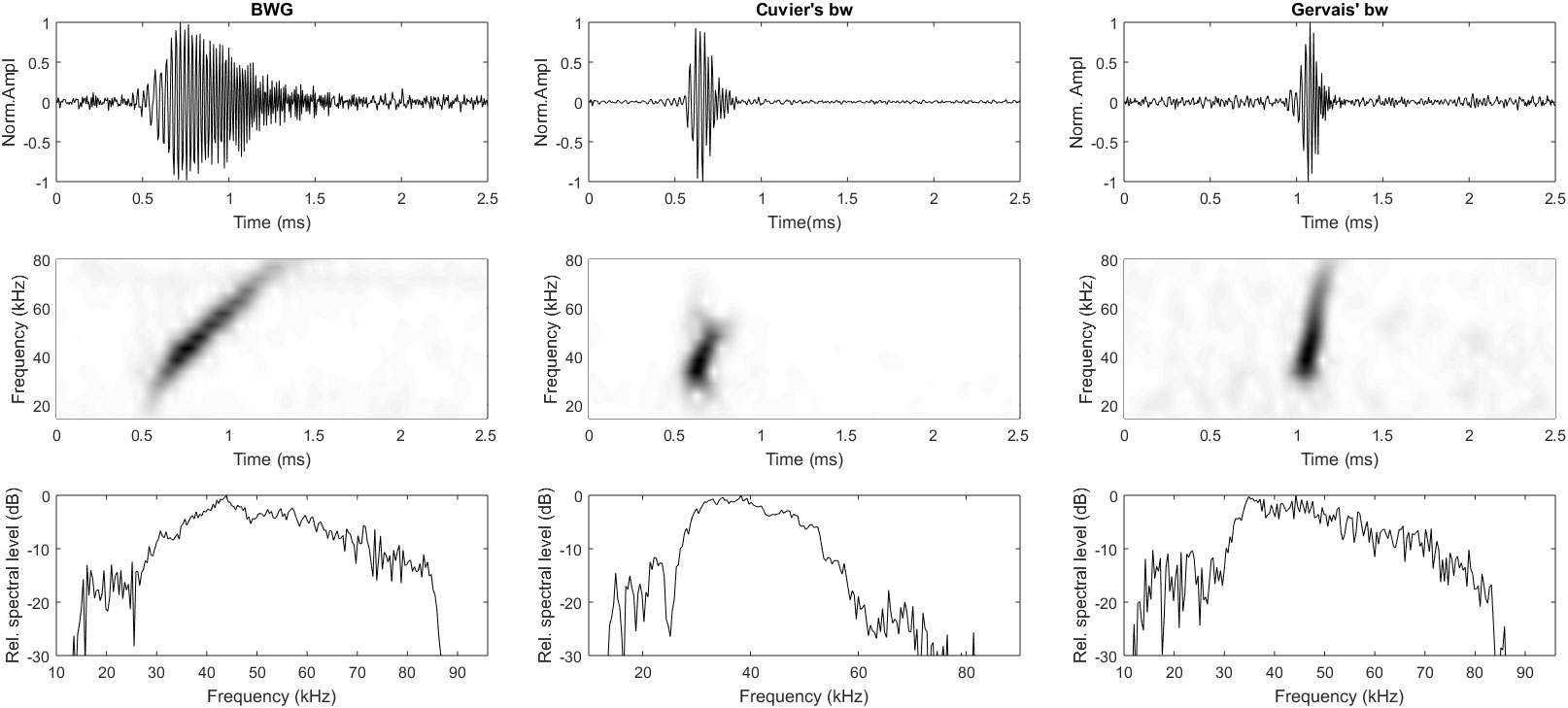
Figure 3 Representative acoustic portraits of three species of beaked whales detected in the Mississippi Canyon area: BWG (first column), Cuvier’s (middle column) and Gervais’ (last column). The upper row is temporal signatures, middle row is spectrograms, and the bottom row is normalized power spectral density levels.

TABLE 4

Table 4 Number and proportion (in %) of detected cues per species per site.

FIGURE 4

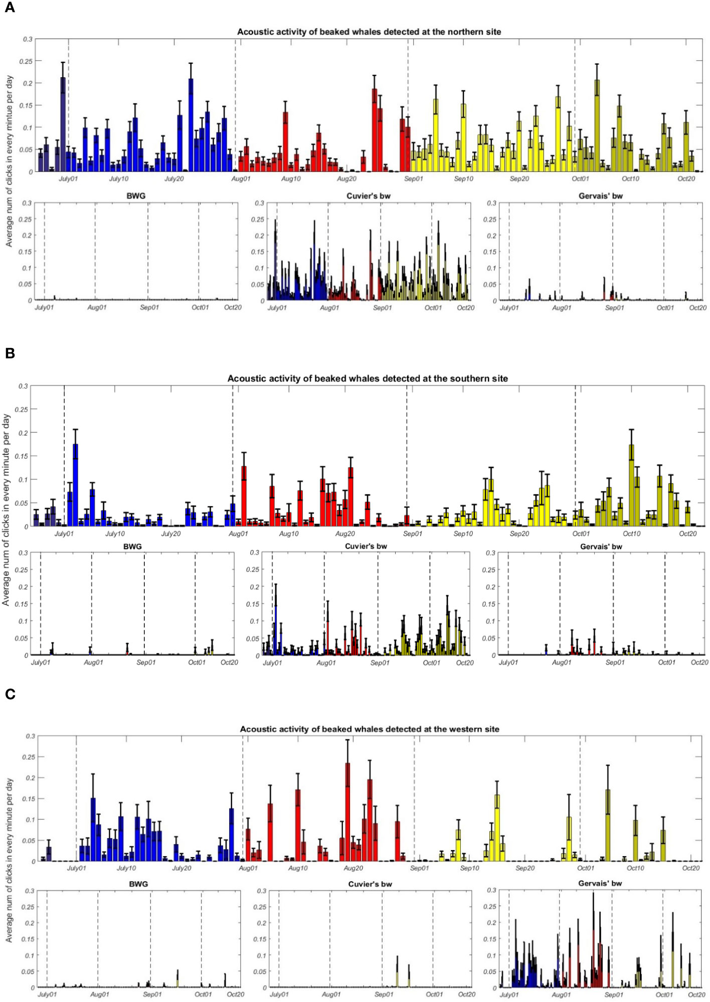
Figure 4 (Top) Average daily click rates of beaked whales detected at the (A) northern (N), (B) southern (S), (C) western (W) sites from June 26 to October 20, 2015. (Bottom) Average daily click rates of BWG, Cuvier’s, and Gervais’ beaked whales at the N, S and W sites. Daily averages and associated standard errors are shown. Colors indicate different months (dark blue, June; blue, July; red, August; yellow, September; green, October).

3.2 Probability of detection

Figure 5 shows the estimated probability-of-detection curves for Cuvier’s and Gervais’ beaked whales as a function of range for the 2015 acoustic dataset. Figure 5 indicates that the estimated maximum detection ranges for Cuvier’s and Gervais’ are about 6 km. The results show that Cuvier’s beaked whale clicks below the range of 1.4 km are certain to be detected; for Gervais’ beaked whale, clicks are certainly detected within the range of 0.7 km. The major factors impacting the maximum detection ranges and probability of detection curves shapes, which are different from previously published ones, are the hydrophone depths and a specific detection algorithm with a dynamic detection threshold.

FIGURE 5

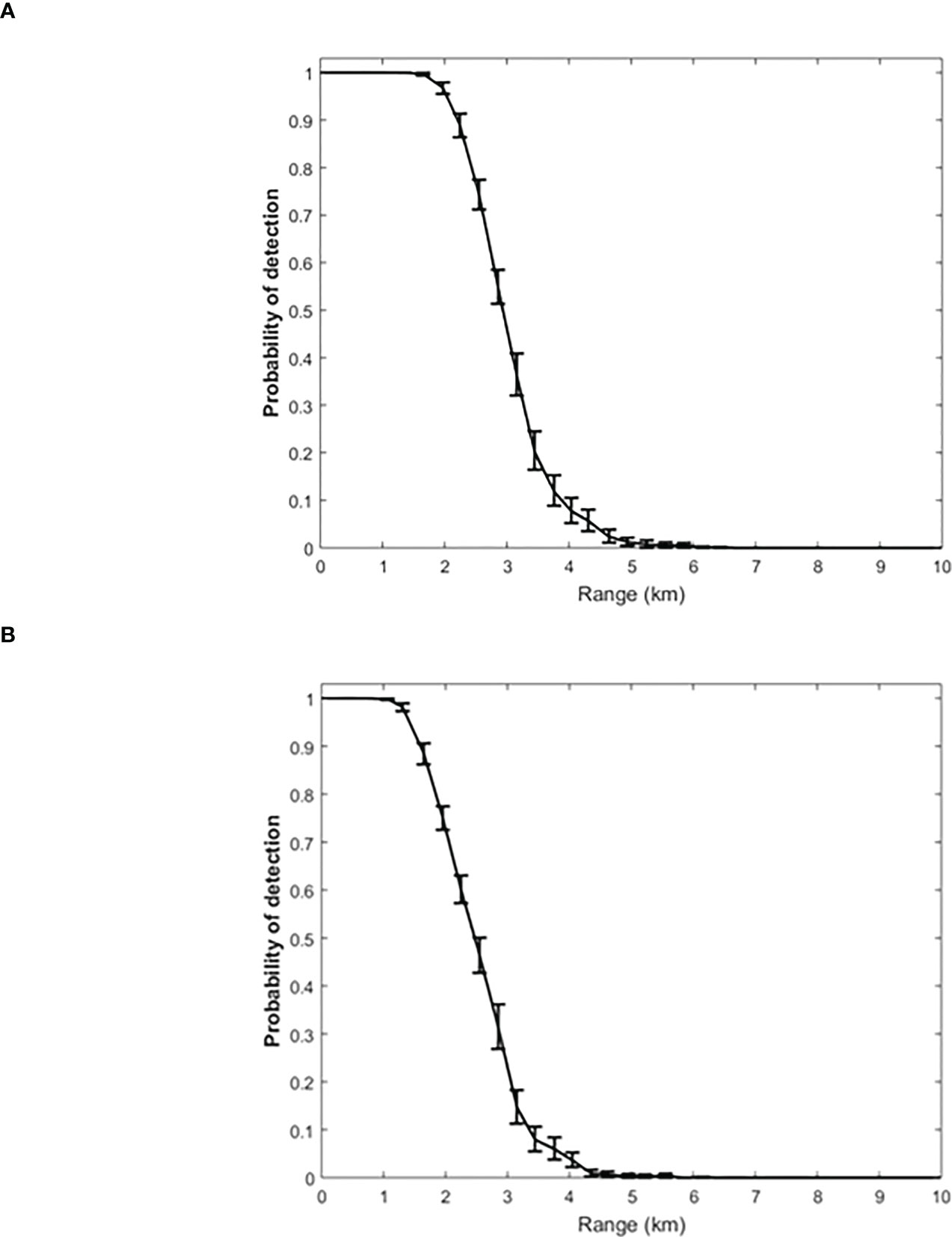
Figure 5 Estimated probability of detection with error bars as a function of range for (A) Cuvier’s and (B) Gervais' beaked whale clicks based on Monte Carlo simulation with the 2015 data set.

3.3 Click production rate

The estimated inter-click intervals (ICIs), click production rate, and associated coefficients of variation (CV) per full dive cycle are listed in Table 5. The different species of beaked whales in GoM have different ICIs, and the ICIs and clicks production rates of both species varied slightly with both time and location. Cuvier’s beaked whale has a longer ICI (544 ms on average) than Gervais’ beaked whale (280 ms on average). The average click production rate for Cuvier’s beaked whale and Gervais’ beaked whale are 0.484 clicks/s and 0.645 clicks/s, respectively. For comparison, the average click production rate for Cuvier’s and Gervais’ beaked whales reported by Hildebrand et al., 2015 were 0.488 and 0.473 clicks/s, respectively, and the production rate for Blainville’s beaked whale estimated by Küsel et al., 2011 was 0.649 clicks/s.

TABLE 5

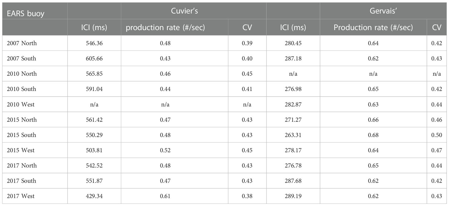
Table 5 Estimated mean inter-click interval (ICI), click production rates and coefficients of variation (CV) for Cuvier’s and Gervais’ beaked whales for each dataset.

3.4 Density trend

To investigate the Cuvier’s and Gervais’ beaked whale local density trends, it is assumed that the local densities in the studied area were not affected by migration between the three sites during the analysis period. The density estimation results for two major species of beaked whales are presented in Tables 6 and 7. Figure 6 shows the average density estimates of Cuvier’s and Gervais’ beaked whales for each site for each survey year. Due to the extremely small proportion of the BWG beaked whales’ calls, we do not make any comparison of the density for the BWG beaked whales across the survey years. From Table 6 , we see that the average density of Cuvier’s beaked whales at the N site increased by 127% from 2007 (in July) to 2010 (in September) at a temporal scale of two-week, and then increased by 176% from 2010 (in September) to 2015 (four-month period), and decreased by 28% from 2015 to 2017 across the same monitoring season. It is very likely that the density of Cuvier’s beaked whales increased in the N site from 2007 to 2015 even with consideration of the short-term temporal observations in 2007 and 2010. At the S site, the densities were slightly increased by 5.4% from 2007 (in July) to 2010 (in September) and increased by 10.3% from 2010 (in September) to 2015 (four-month period), and then decreased by 51.2% from 2015 to 2017. At the W site, the density estimates for Cuvier’s beaked whales are low suggesting that they are not using the site in the foraging dives. For Gervais’ beaked whales, the density at the W site decreased by 54% from 2010 to 2015, and then decreased by 63% from 2015 to 2017. The densities at the N and S sites were relatively small compared to the density at the W site. Large differences in the density estimates between two species are indicative of the regional habitat separation, previously discussed in Li et al. (2020).

TABLE 6

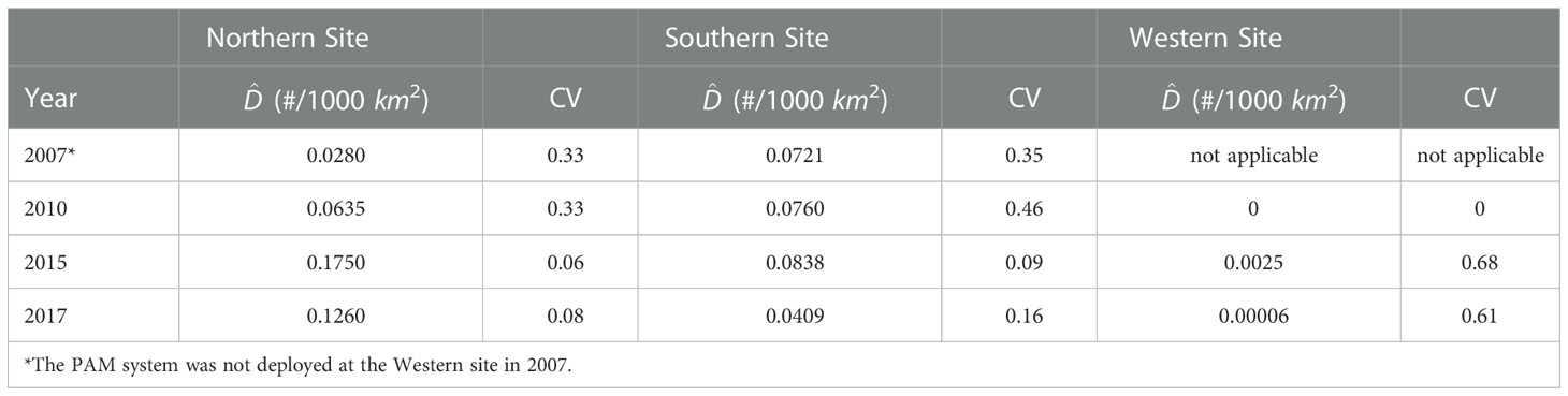
Table 6 Estimated average density of Cuvier’s beaked whales and associated CV obtained by the bootstrap method.

TABLE 7

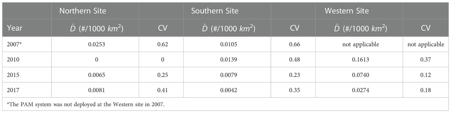
Table 7 Estimated average density of Gervais’ beaked whales and associated CV obtained by the bootstrap method.

FIGURE 6

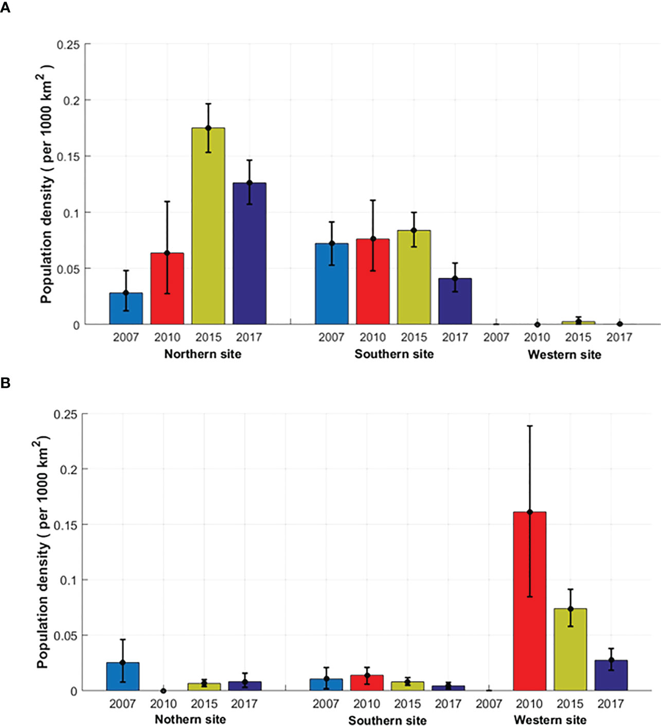
Figure 6 Mean and 95% confidence interval of the estimated density of (A) Cuvier’s and (B) Gervais’ beaked whales.

4 Discussion and conclusions

In this study, the regional site-specific beaked whale density dynamics were investigated using passive acoustic data sampling at three fixed northern GoM sites several times in a decade (2007-2017). This study is the first attempt to provide insights into the long-term regional response of beaked whales to DWH oil spill. The study identified three different species of beaked whales in the region and showed different habitat preference patterns. The results demonstrated that the dominant species in the Mississippi Canyon/Valley area near the spill site (two deeper sites (1500 m)) was Cuvier’s beaked whales. Gervais’ beaked whale species occupied the shallower site (1000 m). While the results support the notion that the two species may have different deep-diving abilities, with Gervais’ beaked whales preferring shallower foraging sites in order to avoid competition, the results also reveal challenges in the design of passive acoustic monitoring surveys for beaked whale density estimates. Such surveys should have a proper spatial resolution to reflect habitat preferences and usage when several competing species are studied. A previously published study (Li et al., 2020) showed that BWG (Baumann-Pickering et al., 2013) beaked whale calls were mostly produced during the night time. At this point, we do not have sufficient information to explain the rarity of these calls. That may be due to the limitations of a fixed sensor’s detection of highly mobile animals or due to the fact that these calls may be uncommon call types produced by known species (more probably by the Gervais’ species due to the highly correlated detection times with the Gervais’ acoustic encounters). The BWG-categorized sounds could be produced by Gervais’ beaked whales exhibiting different acoustic behaviour at night instead of a call of unknown species of beaked whales. Similar results were discussed by Baumann-Picking et al. (2014), based on the analysis of acoustic data from the Cross Seamount using fixed sensors to assess the geographic distribution for different species. Another unknown species, described as BWC, could be produced by the ginkgo-toothed beaked whales present in the area. These two species are occasionally sympatric in the central Pacific (Baumann-Picking et al., 2014). The distribution of M.ginkgodens overlaps with the occurrence of the BWC. Better understanding of the habitat separation among species suggested by our study may help future understanding of the differences in responses of species to ecological stresses.

The detection process used in the study is based on a dynamic detection threshold at the detection step to rule out the possibility of counting bottom reflected clicks which are associated with weaker signals. Beaked whale clicks are highly directional and beaked whales may tend to move between locations to feed at different times of the day, therefore, a beaked whale could swim relative to a fixed sensor in any direction. This will cause click’s amplitude to attenuate rapidly as the off-axis angle increases, which can lead to missed clicks in the detection process.

The animal’s position and orientation for estimating the probability of detection were modelled based on the beaked whale’s diving behaviour during vocal periods following the approach suggested by Küsel et al. (2011). The animal’s position in horizontal plane (x, y) was derived from the assumption that beaked whales are randomly distributed within a circular area of the radius of 10 km centered at the receiver. The animal position could be selected using the uniform probability density function inside the assumed circular area (Buckland et al., 2001) since there is no preferred location bias at our sites within 10 km radius, no considerable environmental/depth changes. This random distribution implies that the distribution of animal distances in horizontal plane is a triangular distribution meaning that more animals are available at a given distance as distances from the hydrophone increases, suggested by Buckland et al., 2001 , and conventionally used for a single hydrophone to estimate the probability of detection from cetacean calls (Küsel et al., 2011; Küsel et al., 2016). Similar research conducted by Hildebrand et al., 2015 also assumes a uniform distribution of animals in the circle around a sensor since no information on preferred direction of travel is available for studied sites. The position in vertical plane (depth/z) was modelled by Gaussian distributions at the preferred foraging depth derived from published literature (Johnston et al., 2004; Küsel et al., 2011; Hildebrand et al., 2015). The animal’s heading (azimuth) was drawn from a uniform distribution (0°-360°) within the assumed circular area. It is noted that the simulation relies on the assumed distributions of these animal’s calls. Within the monitored area, the animal distributions are assumed not to be strongly influenced by oceanographic and geographic features, such as bottom topography, water depth, temperature. However, the complete information is never known in practice, therefore, the modelled distributions could be different from the true animal distributions resulting in potential error for calculation of the probability of detection due to the spatial variability. Alternative approach is to estimate animal’s locations for detected calls and investigate the impact of oceanographic features and prey distribution subject to the availability of both data types. Non-uniform animal’s distributions should be incorporated into the future simulation and their effects should be studied to reduce bias introduced by the assumption of the uniform distributions. Additionally, the multiple fixed sensors deploy in the monitored area on a grid could help understanding the probability of animal’s presence in space. However, this survey type would be more costly. For simulation purposes, due to the long-term period monitoring in our study area, we assumed that the animal positions could be drawn from the uniform probability density function over the monitored area. Future efforts will be conducted to seek for more accurate representation of animal distributions combing with in situ observations to improve the accuracy of the model-based simulation framework.

Our estimated probability-of-detection functions show that clicks from both species can be detected for ranges closer than 0.7-1.4 km with the highest probability (=1). The estimated probability-of-detection functions decline with range. The whales can be detected with a small probability of 0.07 (for Cuvier’s beaked whale) and 0.03 (for Gervais’ beaked whale) at 4 km. The clicks will not be detected beyond 6 km for both species. Several publications have presented different maximum detection ranges and probability-of-detection functions (Zimmer et al., 2008; Marques et al., 2009; Ward et al., 2011; Küsel et al., 2011; Hildebrand et al., 2015). Zimmer et al. (2008) reported the probability of detection for Cuvier’s beaked whale near value of one between 0.7 km and 2.4 km with the maximum detection range of 4 km by using near-surface hydrophone (at a depth of 100 m). The maximum detection range of 6.5 km for Blainville’s beaked whales was previously measured by Ward et al. (2008) using a digital tag (DTag) and distributed bottom-mounted hydrophones. A similar study for Blainville’s beaked whales (M.densirostris) presented by Ward et al. (2011) reported the maximum detection range of approximately 7.8 km for the hydrophone at 1630 m water depth in Bahamas. The study modelled detection difference with increasing ambient noise levels from wind. The probability of detection decreased with increasing ambient noise levels. The detection probabilities were reduced to less than 0.1 for off-axis clicks and 0.18 (at 10.8 m/s wind speed) for on-axis clicks at 4 km. Marques et al. (2009) reported the maximum detection distance of 6.5 km. Hildebrand et al. (2015) reported the beaked whale probability of detection functions with the highest probabilities approximately at ranges below 0.5 km and maximum detection ranges up to 3.2 km and 3.5 km for Gervais’ and Cuvier’s beaked whales, respectively. The distribution of detection probabilities and limits for maximum detection ranges depend on several factors, such as source level of a whale, ambient noise level, depth of the hydrophone, propagation conditions, and automatic algorithm detection threshold (Zimmer et al., 2008). In this study, an 8-min data sample on each hydrophone from each survey year was used to calculate ambient noise level. The ambient noise level may change over time and vary within each year. Considering the potential variations in ambient noise levels, a longer time period of samples from the datasets would be chosen to estimate ambient noise levels for predicting detection probability in future work.

To compare the local density estimates prior and post the DWH oil spill, it is important to address the variability due to the fact that the data collection periods in 2007 and 2010 lasted only two weeks while the data collection periods in 2015 and 2017 were of four months duration. In addition, the experiment in 2007 was in July, and the experiment in 2010 was in September. Furthermore, the W site was not monitored in 2007. The results showed that the change in local density for Cuvier’s beaked whale exhibited an increase near the oil spill site after the spill. That may have led to increased consumption of the polluted prey near the oil spill site and supports future long-term ecological concerns. The reason for the observed increase in local density from 2010, after the oil spill, to 2015 is more likely that there was inter-annual variability in the underlying oceanography which could result in changes in beaked whale migration for prey and food resources within the monitored area. In addition, there are many other factors that may affect beaked whale density in the study area, such as the anthropogenic noise level to which beaked whales are known to be sensitive, fishing activities in the area, long-range seasonal migrations (Cox et al., 2006; Aguilar et al., 2006), and other changes in the environment.

In our study, we observed two patterns in the acoustic activity of beaked whales. First, there is always a clearly dominating beaked whale species at each site. Second, Cuvier’s beaked whales tend to occupy deeper sites, while Gervais’ beaked whales tend to be present in the shallower site. Following the ecological dietary niche hypothesis, Gervais’ beaked whales tend to eat smaller prey and may avoid regions abundant in Cuvier’s beaked whales to reduce competition pressure for prey (MacLeod et al., 2003). Our results indicate that Cuvier’s beaked whales are the dominant species in the region (MC) in terms of acoustic activity and density. That is different from the conclusions presented by Hildebrand et al. (2015) when using similar measures of acoustic activity. The fact that Hildebrand’s single deployment site in the Mississippi Valley area was at the approximate depth of 980 m may have led to different conclusions (Figure 1). In our opinion, the differences in the estimated localized densities are mostly due to Gervais’ species dominating the shallower water site. The differences in the modelled probability of detection as a function of horizontal range are driven by mooring design, particularly by the hydrophone in our study being placed at the preferred foraging depths. The measurements by a sensor placed close to the compact glass platform (as done in the Scripps mooring) may be affected by scattering from the platform. Click counting in our study was based on the dynamic threshold used at the detection stage to eliminate weak and faint calls associated with reflected arrivals to avoid overcounting clicks produced by a single animal. Also, there was uncertainty of the beam pattern effect for off-axis clicks. The question as to whether the beaked whale maintains the upsweep spectral structures for off-axis clicks is still open and was only investigated by a single peer-reviewed article by Guilment et al., 2020. All these factors could explain significant differences in regional densities estimates across different research groups. An additional investigation is required to make a direct comparison of the density estimates across different PAM platforms, which is outside the scope of this paper.

Cue production rate can vary by behavioral state of the whales, resulting in the fact that two species (Cuvier’s and Gervais’ beaked whales) should have spent different portions of times clicking during the deep dive, therefore, the production rates for these two species should be calculated separately using their diving profiles. Due to the lack of tagged data on the vocal duration for Gervais’ beaked whales, we used properties of Blainville’s beaked whales as the proxy for Gervais’ beaked whales due to the similarity in body size and approximation in inter-click interval (ICI). It is noted that our estimated production rate for Cuvier’s beaked whale is consistent with the rate reported by Hildebrand et al., 2015, however, the click production rate for Gervais’ beaked whale was greater than the production rate of Cuvier’s beaked whale. The production rate in our study was similar to the value estimated by Küsel et al., 2011 for Blainville’s beaked whale as we use Blainville’s vocal duration and dive cycle as proxies. The differences come from the estimation of proportion of time clicking during the dive. Due to the unavailability of tagged data for Gervais’ beaked whale, one of the potential errors in estimating the densities of Gervais’s beaked whale result from the need to know the accurate vocal duration, time of a full deep dive foraging cycle, and time of buzz production to obtain accurate estimates of production rate. Gervais’ beaked whale click rates were estimated by Hildebrand et al., 2015 using tag data from a Blainville’s beaked whale recorded in Bahamas as the best available proxy for Gervais’ beaked whales (Hildebrand et al., 2015). For Gervais’ beaked whales, no measurements of diving profiles have been reported in the literature, so the proxies used for Gervais’ beaked whale could be inaccurate, leading to a biased production rate in both GoM studies. One of future efforts should be directed at tagging GoM whales to increase the accuracy of the production rates and region-specific local density estimates.

Roberts et al. (2016) aggregated historical datasets of 16 years (1992-2007), combining both aerial and shipboard surveys, and predicted the maximum density for all beaked whales in GoM was 0.5-6/100 km² (total abundance in the Gulf of Mexico =2019). The averaged beaked whale densities previously estimated by Hildebrand et al., 2015 at the MC site during the 2010-2013 were 0.57/1000 km² for Cuvier’s beaked whale and 3.29/1000 km² for Gervais’ beaked whale. The recent surveys and abundance estimates were conducted by the NOAA’s National Marine Fisheries Service in the northern Gulf of Mexico in 2017 and 2018 (Garrison et al., 2020; NOAA, 2022). The best density and abundance estimate for Cuvier’s beaked whale in 2017 (from July to August) and 2018 (from August to October) were 0.032/1000 km² (11.87 animals) and 0.064/1000 km² (23.56 animals). For comparison, our results show that the estimated average densities of Cuvier’s beaked whale across all three sites (N, S, and W) for two long-term survey years (2015, 2017) were 0.087/1000 km² (32.1 animals), and 0.056/1000 km² (20.7 animals), respectively. These results are corroborated by the report from the NOAA’s National Marine Fisheries Service abundance estimates. For Gervais’ beaked whale our estimated average densities across all three sites for two long-term survey years in 2015 and 2017 were 0.029/1000 km² (10.89 animals) and 0.013/1000 km² (4.8 animals) respectively. Per NOAA’s report, the best abundance estimates for Gervais’ beaked whale were 0/1000 km² (0 animals) in 2017, and 0.11/1000km² (40.39 animals) in 2018. The average estimated abundances across the entire Gulf of Mexico during 2017-2018 for Cuvier’s and Gervais’ beaked whales were 18 (CV=0.75) and 20 (CV=0.98), respectively. Therefore, it appears that the results reported in our study provide reasonable estimates for local densities at the monitoring sites.

Future efforts to understand and reconcile the considerable differences in the beaked whale local density estimates reported in the literature are needed. Special attention in future monitoring efforts should be in four areas: 1) collecting long-term continuous PAM data with spatial resolution allowing for habitat separation and regional and long-range migrations; 2) developing new analysis methods to predict the response of different marine mammal species to changes in oceanographic conditions, deep water prey distribution, and anthropogenic noise level via synthesis of different data types from the same region and time period; 3) tagging regional marine mammals to increase the accuracy of the region-specific local density estimates and 4) benchmarking recording systems and processing tools used by different research teams.

Data availability statement

The processed beaked whale detection data for 2015 and 2017 are publicly available through the Gulf of Mexico Research Initiative Information & Data Cooperative (GRIIDC) at https://data.gulfresearchinitiative.org (doi: 10.7266/N7V69GNZ; doi: 10.7266/n7-4zw6-ap48).

Author contributions

NS conceived the study, designed the experiments, received the funding, and led the field work. SG led system’s calibration, deployment, and recovery in 2010, 2015 and 2017. CT and KL developed the species-specific detection tools and processed the acoustic data. KL, TG and TT developed the density estimation codes. KL, TG, and TT wrote the manuscript draft. NS and CT reviewed the entire manuscript. All authors contributed to the article and approved the submitted version.

Fundings

This research was made possible by a consortium grant from The Gulf of Mexico Research Initiative. The 2010 data collection was made possible in part by a grant from the U.S. National Science Foundation (Grant No. DMS-1059753, 2010-2012).

Acknowledgments

The authors would like to dedicate this work to George E. Ioup’s legacy in the Gulf of Mexico marine mammal acoustic research. Dr. Ioup passed away in January 2016. Dr. Ioup was a founder of deep diving marine mammal acoustic research in the northern Gulf of Mexico and led the LADC-GEMM consortium research between 2000 and 2015. We thank John Hildebrand and Kaitlin Frasier of the SCRIPPS Institute of Oceanography and other colleagues from the bioacoustics community for many fruitful and challenging discussions. We also express our gratitude to Greenpeace for donating the Arctic Sunrise ship time and crew service for the 2010 experiment; SPAWAR for funding the 2007 field work; and LUMCON R/V Pelican crew for providing support of the 2015 and 2017 EARS deployment and recovery.

Conflict of interest

CT is employed by R2Sonic LLC and SG is employed by Proteus Technologies LLC.

The remaining authors declare that the research was conducted in the absence of any commercial or financial relationships that could be construed as a potential conflict of interest.

Publisher’s note

All claims expressed in this article are solely those of the authors and do not necessarily represent those of their affiliated organizations, or those of the publisher, the editors and the reviewers. Any product that may be evaluated in this article, or claim that may be made by its manufacturer, is not guaranteed or endorsed by the publisher.

References

Ackleh A. S., Ioup G. E., Ioup J. W., Ma B., Newcomb J., Pal N., et al. (2012). Assessing the deepwater horizon oil spill impact on marine mammal population through acoustics: Endangered sperm whales. J. Acoust. Soc Am. 131, 2306–2314. doi: 10.1121/1.3682042

PubMed Abstract | CrossRef Full Text | Google Scholar

Aguilar S. N., Johnson M., Madsen P. T., Tyack P. L., Bocconcelli A., Fabrizio B. ,. J. (2006). Does intense ship noise disrupt foraging in deep-diving cuvier's beaked whales (Ziphius cavirostris)? Mar. Mamm. Sci. 22, 690–699. doi: 10.1111/j.1748-7692.2006.00044.x

CrossRef Full Text | Google Scholar

Ainslie M. A., Halvorsen M. B., Robinson S. P. (2022). A terminology standard for underwater acoustics and the benefits of international standardization. IEEE J. Oceanic Eng. 47, 179–200. doi: 10.1109/JOE.2021.3085947

CrossRef Full Text | Google Scholar

Au W. W. L. (1993). The Sonar of Dolphins (New York: Springer‐Verlag), 98–114.

Google Scholar

Au W. W. L., Hastings M. C. (2008). Principles of marine bioacoustics (New York: Springer).

Google Scholar

Baumann-Pickering S., McDonald M. A., Simonis A. E., Berga A. S., Merkens K. P. B., Oleson E. M., et al. (2013). Species-specific beaked whale echolocation signals. J. Acoust. Soc Am. 134, 2293–2301. doi: 10.1121/1.4817832

PubMed Abstract | CrossRef Full Text | Google Scholar

Baumann-Pickering S., Roch M. A., Brownell R. L. Jr., Simonis A. E., McDonald M. A., Solsona-Berga A., et al. (2014). Spatio-temporal patterns of beaked whale echolocation signals in the North Pacific. PLoS One 9, e86072. doi: 10.1371/journal.pone.0086072

PubMed Abstract | CrossRef Full Text | Google Scholar

Buckland S. T., Anderson D. R., Burnham K. P., Laake J. L., Borchers D. L., Thomas L. (2001). Introduction to distance sampling: Estimating abundance of biological populations (Oxford, UK: Oxford University Press).

Google Scholar

Casella G., Berger R. L. (2001). Statistical inference (Boston, MA: Cengage Learning).

Google Scholar

Cox T. M., Ragen T. J., Read A. J., Vos E., Baird R. W., Balcomb K., et al. (2006). understanding the impacts of anthropogenic sound on beaked whales. J. Cetacean Res. Manage. 7, 177–187.

Google Scholar

Dyer S., Pierpoint C., Sidorovskaia N. (2015). ASVs for Passive Acoustic Monitoring: Keeping Track of Marine Wildlife in the Gulf Post-Deepwater Horizon. Sea Technol., 15–18.

Google Scholar

Frantzis A., Goold J. C., Skarsoulis E. K., Taroudakis M. I., Kandia V. (2002). Clicks from cuvier’s beaked whales, Ziphius cavirostris (L). J. Acoust. Soc Am. 112, 34–37. doi: 10.1121/1.1479149

PubMed Abstract | CrossRef Full Text | Google Scholar

Garrison L. P., Ortega-Ortiz J., Rappucci G. (2020). Abundance of marine mammals in waters of the US gulf of Mexico during the summers of 2017 and 2018. Miami, FL: Southeast Fisheries Science Center, 1–56.

Google Scholar

Guilment T., Sidorovskaia N., Li K. (2020). “Modeling the acoustic repertoire of cuvier’s beaked whale clicks”. J. Acoust. Soc Am. 147, 3605–3612. doi: 10.1121/10.0001266

PubMed Abstract | CrossRef Full Text | Google Scholar

Hildebrand J. A., Baumann-Pickering S., Frasier K. E., Trickey J. S., Merkens K. P., Wiggins S. M., et al. (2015). Passive acoustic monitoring of beaked whale densities in the Gulf of Mexico. Sci. Rep. 5, 16343. doi: 10.1038/srep16343

PubMed Abstract | CrossRef Full Text | Google Scholar

Hildebrand J. A., Frasier K. E., Baumann-Pickering S., Wiggins S. M., Merkens K. P., Garrison L. P., et al. (2019). Assessing seasonality and density from passive acoustic monitoring of signals presumed to be from pygmy and dwarf sperm whales in the gulf of mexico. Front. Mar. Sci. 6, 66. doi: 10.3389/fmars.2019.00066

CrossRef Full Text | Google Scholar

Ioup G. E., Ioup J. W., Sidorovskaia N. A., Tiemann C. O., Kuczaj S. A., Ackleh A. S., et al. (2016). “Environmental acoustic recording system (EARS) in the gulf of Mexico,” in Listening in the ocean (New York: Springer), 117–162.

Google Scholar

ISO (2017). 18405, underwater acoustics–terminology (Geneva, Switzerland: International Organization for Standardization).

Google Scholar

Jarvis S., Dimarzio N., Watwood S., Dolan K., Morrissey R. Z. (2022). Automated detection and classification of beaked whale buzzes on bottom-mounted hydrophones. Front. Remote Sens. 82. doi: 10.3389/frsen.2022.941838

CrossRef Full Text | Google Scholar

Johnson M., Madsen P. T., Zimmer W. M., Aguilar De Soto N., Tyack P. L. (2004). Beaked whales echolocate on prey. Proc. R. Soc London. Ser. B: Biol. Sci. 271, S383–S386. doi: 10.1098/rsbl.2004.0208

CrossRef Full Text | Google Scholar

Johnson M., Madsen P. T., Zimmer W., De Soto N. A., Tyack P. (2006). Foraging blainville’s beaked whales (Mesoplodon densirostris) produce distinct click types matched to different phases of echolocation. J. Exp. Biol. 209, 5038–5050. doi: 10.1242/jeb.02596

PubMed Abstract | CrossRef Full Text | Google Scholar

Küsel E. T., Mellinger D. K., Thomas L., Marques T. A., Moretti D., Ward J. (2011). Cetacean population density estimation from single fixed sensors using passive acoustics. J. Acoust. Soc Am. 129, 3610–3622. doi: 10.1121/1.3583504

PubMed Abstract | CrossRef Full Text | Google Scholar

Küsel E. T., Siderius M., Mellinger D. K. (2016). Single-sensor, cue-counting population density estimation: Average probability of detection of broadband clicks. J. Acoust. Soc. Am. 140, 1894–1903. doi: 10.1121/1.4962753

PubMed Abstract | CrossRef Full Text | Google Scholar

Li K., Sidorovskaia N. A., Guilment T., Tang T., Tiemann C. O. (2021). Decadal assessment of sperm whale site-specific abundance trends in the northern Gulf of Mexico using passive acoustic data. J. Mar. Sci. Eng. 454, 1–17. doi: 10.3390/jmse9050454

CrossRef Full Text | Google Scholar

Li K., Sidorovskaia N., Tiemann C. (2020). Model-based unsupervised clustering for distinguishing cuvier’s and gervais’ beaked whales in acoustic data. Ecol. Inform 58, 1–19. doi: 10.1016/j.ecoinf.2020.101094

CrossRef Full Text | Google Scholar

Love M., Baldera A., Robbins C., Spies R. B., Allen J. R. (2015). Charting the gulf: Analyzing the gaps in long-term monitoring of the gulf of mexico. New Orleans LA: Ocean. Conserv. 1–102. Available from: www.oceanconservancy.org/gapanalysis.

Google Scholar

MacLeod C. D., Santos M. B., Pierce G. J. (2003). Review of data on diets of beaked whales: evidence of niche separation and geographic segregation. J. Mar. Biolog. Assoc. U.K. 83, 651–665. doi: 10.1017/S0025315403007616h

CrossRef Full Text | Google Scholar

Marques T. A., Thomas L., Ward J., DiMarzio N., Tyack P. L. (2009). Estimating cetacean population density using fixed passive acoustic sensors: An example with blainville’s beaked whales. J. Acoust. Soc Am. 125, 1982–1994. doi: 10.1121/1.3089590

PubMed Abstract | CrossRef Full Text | Google Scholar

Marques T. A., Thomas L., Ward J., DiMarzio N., Tyack P. L. (2013). Estimating animal population density using passive acoustics. Biol. Rev. 88, 287–309. doi: 10.1111/brv.12001

CrossRef Full Text | Google Scholar

McNutt M. K., Chu S., Lubchenco J., Hunter T., Dreyfus G., Murawski S. A., et al. (2012). Applications of science and engineering to quantify and control the deepwater horizon oil spill. Proc. Natl. Acad. Sci. 109, 20222–20228. doi: 10.1073/pnas.1214389109

CrossRef Full Text | Google Scholar

Moretti D., Marques T. A., Thomas L., DiMarzio N., Dilley A., Morrissey R., et al. (2010). A dive counting density estimation method for blainville’s beaked whale (Mesoplodon densirostris) using a bottom-mounted hydrophone field as applied to a mid-frequency active (MFA) sonar operation. Appl. Acoust. 71, 1036–1042. doi: 10.1016/j.apacoust.2010.04.011

CrossRef Full Text | Google Scholar

NMFS [National Marine Fisheries Service] (2021). U. S. Atlantic and gulf of Mexico marine mammal stock assessment reports – GERVAIS'BEAKED WHALE (Mesoplodon europaeus): Northern gulf of Mexico stock. 1–8. Available from: https://media.fisheries.noaa.gov/2021-07/f2020_AtlGmexSARs_GMexGervais.pdf?null.

Google Scholar

NOAA technical memorandum NMFS-NE (2022). U.S. Atlantic and Gulf of Mexico Marine Mammal Stock Assessments 2021 Eds Hayes S. H., Josephson E., Maze-Foley K., Rosel P. E., Wallace J. (U.S.: Northeast Fisheries Science Center), 288 pp. doi: 10.25923/6tt7-kc16

CrossRef Full Text | Google Scholar

Powell L. A. (2007). Approximating variance of demographic parameters using the delta method: a reference for avian biologists. Condor 109, 949–954. doi: 10.1093/condor/109.4.949

CrossRef Full Text | Google Scholar

Quick N. J., Cioffi W. R., Shearer J. M., Fahlman A., Read A. J. (2020). Extreme diving in mammals: first estimates of behavioural aerobic dive limits in cuvier's beaked whales. J. Exp. Biol. 223, jeb222109. doi: 10.1242/jeb.222109

PubMed Abstract | CrossRef Full Text | Google Scholar

Robbins J. R., Bell E., Potts J., Babey L., Marley S. A. (2022). Likely year-round presence of beaked whales in the bay of biscay. Hydrobiologia 849, 2225–2239. doi: 10.1007/s10750-022-04822-y

CrossRef Full Text | Google Scholar

Roberts J. J., Best B. D., Mannocci L., Fujioka E. I., Halpin P. N., Palka D. L., et al. (2016). Habitat-based cetacean density models for the U.S. Atlantic and Gulf of Mexico. Sci. Rep. 6, 22615. doi: 10.1038/srep22615

PubMed Abstract | CrossRef Full Text | Google Scholar

Schorr G. S., Falcone E. A., Moretti D. J., Andrews R. D. (2014). First long-term behavioral records from cuvier’s beaked whales (Ziphius cavirostris) reveal record-breaking dives. PLoS One 9, e92633. doi: 10.1371/journal.pone.0092633

PubMed Abstract | CrossRef Full Text | Google Scholar

Seber G. A. F. (1982). The estimation of animal abundance and related parameters, 2nd ed. MacMillan Press, New York, USA.

Google Scholar

Sidorovskaia N. A., Ioup G. E., Ioup J. W., Caruthers J. W. (2004). Acoustic propagation studies for sperm whale phonation analysis during LADC experiments. In AIP Conf. Proc. 728, 288–295. doi: 10.1063/1.1843023

CrossRef Full Text | Google Scholar

Sidorovskaia N.. (2019). Eavesdropping on the Gulf of Mexico. Environment Coastal & Offshore, Special Issue “Ocean Sound”, 68–71.

Google Scholar

Takeshita R., Sullivan L., Smith C., Collier T., Hall A., Brosnan T., et al. (2017). The deepwater horizon oil spill marine mammal injury assessment. Endangered Species Res. 33, 95–106. doi: 10.3354/esr00808

CrossRef Full Text | Google Scholar

Tyack P. L., Johnson M., Soto N. A., Sturlese A., Madsen P. T. (2006). Extreme diving of beaked whales. J. Exp. Biol. 209, 4238–4253. doi: 10.1242/jeb.02505

PubMed Abstract | CrossRef Full Text | Google Scholar

Urick R. J. (1983). Principles of underwater sound 3rd edition (California: Peninsula Publishing Los Atlos).

Google Scholar

Würsig B. (2017). “Marine Mammals of the Gulf of Mexico,” In Ward C. Eds. Habitats and Biota of the Gulf of Mexico: Before the Deepwater Horizon Oil Spill (New York, NY: Springer). doi: 10.1007/978-1-4939-3456-0_5

CrossRef Full Text | Google Scholar

Ward J., Jarvis S., Moretti D., Morrissey R., DiMarzio N., Johnson M., et al. (2011). Beaked whale (Mesoplodon densirostris) passive acoustic detection in increasing ambient noise. J. Acoust. Soc Am. 129, 662–669. doi: 10.1121/1.3531844

PubMed Abstract | CrossRef Full Text | Google Scholar

Ward J., Morrissey R., Moretti D., DiMarzio N., Jarvis S., Johnson M., et al. (2008). Passive acoustic detection and localization of Mesoplodon densirostris (Blainville’s beaked whale) vocalizations using distributed bottom-mounted hydrophones in conjunction with a digital tag (DTag) recording. Can. Acoust. 36, 60–66.

Google Scholar

Waring G. T., Josephson E., Maze-Foley K., Rosel P. E. (2011). U.S. Atlantic and Gulf of Mexico marine mammal stock assessments–2010. NOAA Tech Memo NMFS NE 219, 02543–01026.

Google Scholar

Warren V. E., Marques T. A., Harris D., Thomas L., Tyack P. L., Aguilar de Soto N., et al. (2017). Spatio-temporal variation in click production rates of beaked whales: Implications for passive acoustic density estimation. J. Acoust. Soc Am. 141, 1962–1974. doi: 10.1121/1.4978439

PubMed Abstract | CrossRef Full Text | Google Scholar

Zimmer W. M., Harwood J., Tyack P. L., Johnson M. P., Madsen P. T. (2008). Passive acoustic detection of deep-diving beaked whales. J. Acoust. Soc Am. 124, 2823–2832. doi: 10.1121/1.2988277

PubMed Abstract | CrossRef Full Text | Google Scholar

Zimmer W. M. X., Johnson M. P., Madsen P. T., Tyack P. L. (2005). Echolocation clicks of free-ranging cuvier’s beaked whales (Ziphius cavirostris). J. Acoust. Soc Am. 117, 3919–3927. doi: 10.1121/1.1910225

PubMed Abstract | CrossRef Full Text | Google Scholar