Improving multi-decadal coastal shoreline change predictions by including model parameter non-stationarity

Our ability to predict sandy shoreline evolution resulting from future changes in regional wave climates is critical for the sustainable management of coastlines worldwide. To this end, the present generation of simple and efficient semi-empirical shoreline change models have shown good skill at predicting shoreline changes from seasons up to several years at a number of diverse sites around the world. However, a key limitation of these existing approaches is that they rely on time-invariant model parameters, and assume that beaches will evolve within constrained envelopes of variability based on past observations. This raises an interesting challenge because the expected future variability in key meteocean and hydrodynamic drivers of shoreline change are likely to violate this ‘stationary’ approach to longer-term shoreline change prediction. Using a newly available, multi-decadal (28-year) dataset of satellite-derived shorelines at the Gold Coast, Australia, this contribution presents the first attempt to improve multi-decadal shoreline change predictions by allowing the magnitude of the shoreline model parameters to vary in time. A data assimilation technique (Ensemble Kalman Filter, EnKF) embedded within the well-established ShoreFor shoreline change model is first applied to a 14-year training period of approximately fortnightly shoreline observations, to explore temporal variability in model parameters. Then, the magnitudes of these observed non-stationary parameters are modelled as a function of selected wave climate covariates, representing the underlying seasonal to interannual variability in wave forcing. These modelled time-varying parameters are then incorporated into the shoreline change model and tested over the complete 28-year dataset. This new inclusion of non-stationary model parameters that are directly modelled as a function of the underlying wave forcing and corresponding time scales of beach response, is shown to outperform the multi-decadal predictions obtained by applying the conventional stationary approach (RMSE_{non-stationary} = 11.1 m; RMSE_stationary = 254.3 m). Based on these results, it is proposed that a non-stationary approach to shoreline change modelling can reduce the uncertainty associated with the misspecification of physical processes driving shoreline change and should be considered for future shoreline change predictions.

1 Introduction

Sandy coastlines vary at time scales of individual storms to longer-term variability due to changes in waves, water levels, and sediment supply (Vitousek et al., 2017a; Jackson and Short, 2020). Reliable predictions of shoreline evolution that span this range of time scales, both now and by the end of the century, are required for assessing coastal vulnerability in a changing climate (Ranasinghe, 2020; Toimil et al., 2020). This is particularly important given the uncertainty and possible changes in regional wave climates and/or ocean water levels due to climate variability that have the potential to influence the coast (Wong et al., 2014; Ranasinghe, 2016; Vousdoukas et al., 2020; Odériz et al., 2022). As such, significant research effort has been directed towards the development of relatively simple and efficient semi-empirical shoreline change models to predict shoreline evolution over time scales ranging from seasons to decades (e.g., Miller and Dean, 2004; Castelle et al., 2014; Jaramillo et al., 2020; Roelvink et al., 2020; Yates et al., 2009; Splinter et al., 2014; Vitousek et al., 2017b). These models are now being used to explore shoreline changes that may occur during the 21^st century (e.g., Toimil et al., 2017; Vitousek et al., 2017b; D’Anna et al., 2021; D’Anna et al., 2022) assuming that beaches will evolve within constrained envelopes of variability based on past measurements (Luijendijk et al., 2018; Vousdoukas et al., 2020). However, the expected future changes in key meteocean and hydrodynamic drivers of shoreline evolution (e.g., Wong et al., 2014; Morim et al., 2019) suggest that predictive models of longer-term shoreline changes should also include the capability to adapt to changing wave forcing, as well as corresponding time scales of shoreline response (Montaño et al., 2021; Schepper et al., 2021; Splinter and Coco, 2021).

Semi-empirical shoreline change models are simplified representations of the complex sediment transport processes occurring between the shoreface and beach face, and therefore inherit uncertainties from the imprecise representation of physical processes in the model structure and from the forcing inputs (Le Cozannet et al., 2019; Le Cozannet et al., 2016; Kroon et al., 2020; Montaño et al., 2020; D’Anna et al., 2021; Toimil et al., 2021; Vitousek et al., 2021). This misspecification of physical processes is typically addressed via site-specific model calibration, whereby a set of stationary (or time-invariant) model parameters are optimized for a specific time period using observed forcing and co-located shoreline data (Long and Plant, 2012; Splinter et al., 2013). For example, Yates et al. (2011, 2009) applied a semi-empirical cross-shore shoreline model to five beaches in California (USA) spanning up to 5 years of data and found inter-site variability in the magnitude of their four model parameters. Splinter et al. (2014) applied a different cross-shore shoreline change model to datasets obtained from seven diverse beaches across the USA, Europe and Australia, each spanning more than 5 years. These authors similarly found large inter-site variability between the magnitude of model parameters.

In addition to site-specific dependencies on model parameter calibration, recent research suggests that the calibration period and associated characteristics of the wave climate may also introduce parameter biases (D’Anna et al., 2022, D’Anna et al., 2020; Ibaceta et al., 2020; Montaño et al., 2020). For instance, Splinter et al. (2017) analysed 8 years of wave and shoreline observations at the Gold Coast, Australia, finding a substantial difference in optimized model parameters between two independently calibrated 4-year time periods. This was shown to be consistent with a relatively subtle difference in the annual distribution of storm wave events during each of the two consecutive 4-year observation periods. More recently, D’Anna et al. (2022) used a climate-based wave emulator to produce ensemble-based past and future projections of shoreline evolution spanning the 21^st century at Truc Vert, France. Using two different semi-empirical shoreline change models, it was shown that different wave chronologies produced by the emulator can significantly alter the modelled shoreline response. Based on these findings, the authors advocated for more research into the underlying link(s) between model parameters and wave climate variability.

To achieve this objective, data assimilation techniques offer the possibility to estimate non-stationary (i.e., time-varying) parameters and explore their links to changes in natural forcing (Pathiraja et al., 2018; Deng et al., 2019, Pathiraja et al., 2016a; Xiong et al., 2019; Zeng et al., 2019). More specifically, Kalman filter variants (Kalman, 1960) are data assimilation techniques that are already employed in semi-empirical shoreline change modelling to assist with model calibration (e.g., Long and Plant, 2012; Vitousek et al., 2017b; Muir et al., 2020; Alvarez-Cuesta et al., 2021a). By this approach model parameters are continually adjusted as additional state (i.e., shoreline) observations become available (Evensen, 2009). Optimized shoreline predictions are achieved by efficiently weighting and combining the spread of the shoreline observations (represented by the shoreline measurement accuracy) with the spread of the model simulations (referred to as ‘parameter process-noise’). Most commonly, these existing applications have used a Kalman filter to estimate the stationary (i.e., time-invariant) magnitude of shoreline model parameters, by assuming a very low level of parameter process-noise (Vitousek et al., 2017b; Alvarez-Cuesta et al., 2021b; Vitousek et al., 2021). However, Ibaceta et al. (2020) presented a dual state-parameter Ensemble Kalman Filter (EnKF) variant (Pathiraja et al., 2016a, Pathiraja et al., 2016b) and showed its suitability to explore non-stationary, or time-varying parameters within the context of the established cross-shore shoreline change model, ShoreFor (Davidson et al., 2013; Splinter et al., 2014). Specifically, it was found that using a sufficiently high magnitude of parameter process-noise, the EnKF was able to track non-stationary parameters as demonstrated by several synthetic scenarios that were designed to emulate differing modes of shoreline behaviour. The method was also applied to an 8-year real-world shoreline dataset presented in Splinter et al. (2017), that – as was previously noted above - exhibited a distinct shift in shoreline behaviour. In this prior work the EnKF technique successfully reproduced the observed shift in shoreline behaviour and revealed that the resulting non-stationary model parameters were related to changing characteristics of the wave forcing. While this application was limited to past periods where shoreline observations were available for data assimilation, the next challenge is to investigate strategies for extrapolating the detected time-varying parameters out of the training period where the EnKF is applied. To this end, the recent availability of longer and publicly available satellite-derived shoreline datasets (Luijendijk et al., 2018; Vos et al., 2019b; Almeida et al., 2021; Castelle et al., 2021) offers for the first time the opportunity to significantly expand the application of the EnKF methodology, with a particular focus on future shoreline change predictions under climate projections where multi-year variability in wave climate forcing is expected (e.g., D’Anna et al., 2021).

In this work, the EnKF technique that was introduced in Ibaceta et al. (2020) is now applied to an extended multi-decadal dataset of satellite-derived shorelines at the Gold Coast, Australia. As described in Section 2 (Methodology), the technique is first used to estimate the magnitude of non-stationary parameters when applied to the established cross-shore shoreline change model, ShoreFor (Davidson et al., 2013; Splinter et al., 2014). Importantly, the magnitude of these time-varying parameters is then physically related and numerically parametrized as a function of the multi-year variability in wave forcing. Using these new insights, Section 3 incorporates the results of this EnKF time-varying model parameter estimation to predict nearly three decades of observed shoreline changes at the Gold Coast. A comparison of these newly obtained results to the more common ‘stationary’ modeling approach is discussed in Section 4, along with a discussion of the physical interpretation of time-varying model parameters.

2 Methodology

2.1 Study site and data

The Gold Coast is located on the east coast of Australia (Figure 1A). This region spans ~30 km of relatively straight, open-coast sandy beaches characterized by energetic intermediate beach states that typically exhibit double-barred morphology (van Enckevort et al., 2004; Price and Ruessink, 2011). Beach sediments have a median grain size of 0.25 mm and tides are microtidal with mean spring tidal range of 1.5 m (Davidson and Turner, 2009; Splinter et al., 2017). The predominant direction of wave incidence is from S to SE directions, with mean offshore significant wave height (H_s) and spectral peak wave periods (T_p) of 1.1 m and 9.4 s, respectively (Davidson and Turner, 2009). The wave climate of this region generally displays a seasonal nature with more easterly (and smaller) waves in the summer and more southerly (larger) waves in the winter (Zarifsanayei et al., 2022). In general, this results in a seasonal response to shoreline variability as well, with more accreted beaches in the summer and more eroded beaches in the winter that are also modulated at interannual time scales by changes in storminess patterns (Splinter et al., 2017). At interannual time scales, the wave climate is also modulated by the El Niño-Southern Oscillation (Phinn and Hastings, 1995; Barnard et al., 2015).

FIGURE 1

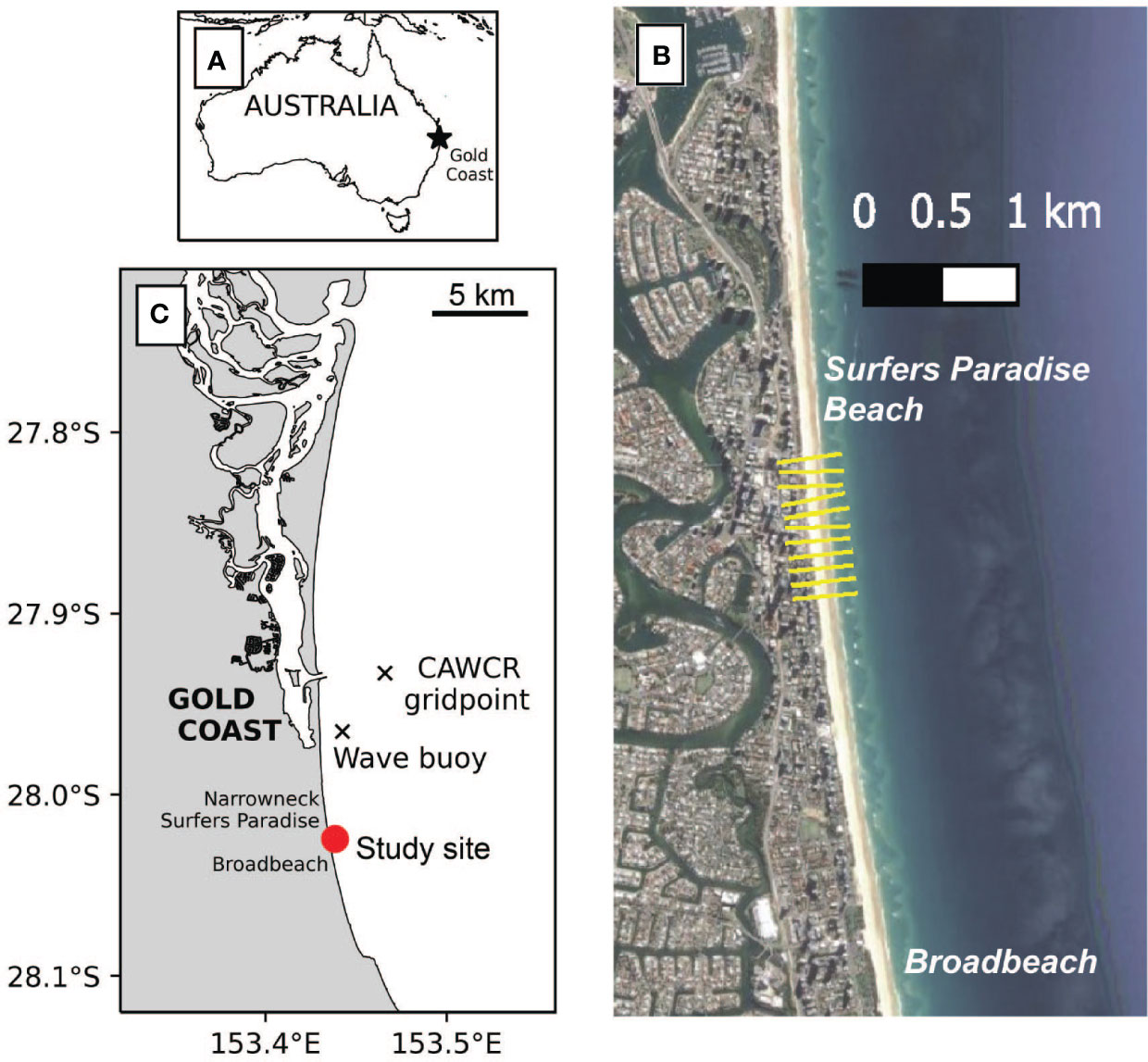
Figure 1 Study site and data. (A) Location of the Gold Coast on the east coast of Australia. (B) Satellite image (source: Google Earth) of the study site and the location of ten shore-normal transects (yellow lines) used for extraction of satellite-derived shoreline time series. (C) Map of the Gold Coast location showing specific location of the study site (red point). Black crosses indicate the location of the waverider buoy and the CAWCR gridpoint used to fill gaps in wave measurements.

Time series of three-hourly wave data (H_s and T_p) are available from a waverider buoy located approximately 4 km to the north and 2 km offshore of the study site in 17 m water depth (Figure 1C). Gaps in the wave buoy time series were filled using values from the closest grid point of the CAWCR reanalysis dataset (Durrant et al., 2014, see Figure 1C). A comprehensive assessment of this wave dataset quality for the Australian region is presented in Hemer et al. (2017).

The portion of coastline examined in this work coincides with the same stretch of coast that was previously analysed over shorter time periods by Splinter et al. (2017) and Ibaceta et al. (2020). Specifically, a 1 km stretch of sandy beach at Surfers Paradise (Figure 1B) was selected. Previous investigations showed that this stretch of coastline is outside the influence of down-drift engineering interventions (Turner, 2006), including the construction of an artificial reef and the placement of a sand nourishment (Boak et al., 2000; Black and Mead, 2001; Turner, 2006). And importantly, Splinter et al. (2011) also showed that minimal gradients of alongshore sediment transport have been observed at this location, necessary for the assumptions of the cross-shore shoreline change model used here (Section 2.2).

The CoastSat toolbox (Vos et al., 2019b) was used to extract satellite-derived shorelines at ten shore-normal transects spaced every 100 m alongshore (Figure 1B, yellow lines). Briefly, CoastSat retrieves time series of cross-shore shoreline position (accuracy ~10-15 m) at any sandy beach from 30+ years of publicly available satellite imagery (Landsat 5,7, 8 and Sentinel 2) at a revisit period of ~2 weeks. At the Gold Coast, 28 years of suitable satellite imagery is available spanning the period 1992-2020. To remove high-frequency shoreline changes related to tidal variations, the resulting time series at each transect were tidally corrected to a fixed datum (MSL) using water levels from a global tide model and an average beach slope (Vos et al., 2020). An average beach slope was used in line with previous studies on satellite-derived shorelines, where using a time-evolving beach slope did not result in better shoreline mapping (Castelle et al., 2021). The reader is referred to Vos et al. (2021) for further details on this dataset.

As the final step in shoreline data pre-processing, the resulting 28-year time series of tidally corrected shorelines were alongshore-averaged over the 1 km long study site, to remove the effect of smaller-scale shoreline features such as beach cusps, commensurate to previous studies at this same site (e.g., Splinter et al., 2017).

Figure 2 summarizes the complete 28-year wave and shoreline Gold Coast dataset. In Figure 2A the wave data is represented by the single parameter dimensionless fall velocity, Ω = H_s,b/wT_p, where w is the sediment fall velocity, which in turn is a function of the site-specific median grain size (i.e., d₅₀ = 0.25 mm). T_p is the 3-hourly peak wave period measured at the wave buoy, and the significant breaking wave height (H_s,b) is estimated from the 3-hourly offshore conditions by reverse-shoaling of the inshore (17 m depth) wave buoy data (after Splinter et al., 2014). In summary, a clear seasonality in the Gold Coast wave climate is evident (Figure 2A), and in addition to this, calculation of the 5-year backwards running mean of Ω (i,e., $\overline{\Omega }$) also reveals longer-term interannual wave climate variability (Figure 2B). The corresponding alongshore-averaged shoreline time series is shown in Figure 2C. Of relevance to this work, both seasonal and interannual shoreline changes are evident during the 1992-2020 period with the shoreline position negatively correlated with the multi-year wave climate variability $\overline{\text{Ω},}$ (r = - 0.3, p< 0.01). The previously identified links between $\overline{\Omega }$ and model parameters of the ShoreFor shoreline change model (Splinter et al., 2014) are now investigated and quantified in the following sections.

FIGURE 2

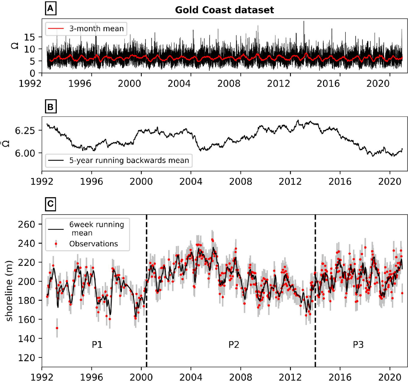
Figure 2 Wave and shoreline datasets. (A) Time series of dimensionless fall velocity spanning the 1992-2020 period (black line). The red line is the 3-month running mean. (B) Interannual variability of the dimensionless fall velocity, here represented by a 5-year running backwards mean. (C) Time series of shoreline evolution at the Gold Coast relative to a local datum. This data was obtained from satellite-derived shorelines (red dots with grey error bars representing the accuracy of the satellite-derived shorelines, here given by R =10 m). The black line is the 6-week centered running mean used to facilitate visualization of the seasonal to interannual variability at this study site. The dataset is split into 3 different time periods (P1, P2, P3). P2 is used for training and all three are used for testing purposes.

2.2 Shoreline change model: ShoreFor

The generalized version of the semi-empirical shoreline change model, ShoreFor (Splinter et al., 2014) is used in the present study to model cross-shore driven shoreline evolution at the Gold Coast study site. ShoreFor is based on the behavioural concept that shorelines continuously evolve towards a time-varying equilibrium position (Davidson et al., 2013), with the cross-shore rate of shoreline change (dx/dt) given by:

$\begin{array}{ll}\frac{dx}{dt}=c^a{F}^a+c^e{F}^e+b& (1)\end{array}$

In this formulation, the forcing term F^a,e = P^0.5ΔΩ_a,e/σ_ΔΩ F^a,e is a function of the wave power at the breaking point (P) and the disequilibrium dimensionless fall velocity (ΔΩ). The wave power at the breaking point is calculated as P = $\raisebox{1ex}{$1$}\!\left/ \!\raisebox{-1ex}{$16$}\right.\rho g{H}_{\mathrm{s,\; b}}^2\sqrt{g{h}_b}$ assuming a breaking criterion h_b = H_s,b/0.78 (Splinter et al., 2014). The variables ρ, g are the water density and acceleration due to gravity, respectively. Importantly, the disequilibrium dimensionless fall velocity (ΔΩ) dictates the potential direction of cross-shore sediment transport as either offshore (ΔΩ_e,when ΔΩ< 0) during erosive conditions or onshore (ΔΩ_a,for ΔΩ > 0) during accretionary conditions. From this, the disequilibrium component ΔΩ = (Ω_eq - Ω) and its associated standard deviation σ_ΔΩ are computed from the 3-hourly dimensionless fall velocity $\text{Ω}=\raisebox{1ex}{$H_{s,b}$}\!\left/ \!\raisebox{-1ex}{$T_{p}w$}\right.$ at the wave breaking point, where T_p is the peak wave period and w is the sediment fall velocity. The time-varying equilibrium expression (after Wright et al., 1985) is given by:

$\begin{array}{ll}{\text{Ω}}_{\text{eq}}={\left[\sum _{i=1}^{2\varphi }{10}^{-i/\varphi }\right]}^{-1}\sum _{i=1}^{2\varphi }{\text{Ω}}_{\text{i}}{10}^{-i/\varphi } & (2)\end{array}$

Of particular relevance to the new work presented here is the physical interpretation of the underlying model parameters in Equation 1. These include three wave-driven cross-shore sediment transport-related parameters c^a, c^e and ϕ that in this study are estimated and permitted to vary independently using the EnKF technique (as described in Section 2.3 below). The two rate parameters c^a and c^e (units: m^1.5s^-1W^-0.5) are proxies for the accretion/erosion sediment transport efficiency and the response factor parameter ϕ (in days) represents a beach response time. This model parameter (ϕ) has also been described as a proxy for ‘beach memory’ as it represents the time length to which predicted shorelines ‘remember’ antecedent wave conditions (Vitousek et al., 2021).

Based on previous testing of the ShoreFor model at a diverse range of seasonal and storm-dominated sandy coastlines in Australia, Europe and the USA, Splinter et al. (2014) showed that the magnitude of these parameters can be related to the mean interannual (≥ 5 years) dimensionless fall velocity $\overline{\text{Ω}}$ (e.g., Figure 2B), consistent with well-established relationships (e.g., Wright and Short, 1984) between modal beach states and cross-shore processes. Conceptually, mild-slope beaches experience slower rates of shoreline changes (i.e., ϕ > 100 days) and decreased sediment exchange efficiency (lower c^a and c^e values) between the surf zone and beach face. Conversely, the breaker line tends to be closer to the beach face at steeper beaches, enhancing efficient (larger c^a and c^e magnitudes) and rapid (i.e., ϕ < 100 days) sediment exchange. Note that the additional b term in Equation 1 is a residual term accounting for any unresolved processes. The reader is referred to Splinter et al. (2014) and Davidson et al. (2013) for a full description and formulation of the ShoreFor model.

2.3 Shoreline modelling with non-stationary parameters

The new methodology that is developed here for predicting shoreline change using non-stationary parameters is comprised of four steps:

(1) Non-stationary model parameters are estimated using the EnKF methodology presented in Ibaceta et al. (2020). The same EnKF algorithm is also tuned to calculate stationary (i.e., time-invariant) or ‘converged’ parameters (e.g., Long and Plant, 2012; Vitousek et al., 2017b) to compare with this new non-stationary approach;

(2) Correlation analyses between estimated non-stationary parameters and wave forcing covariates (e.g., $\overline{\text{Ω}}$) are undertaken using the Pearson correlation coefficient (r).;

(3) Linear regression is used to develop expressions of the non-stationary parameters based on the results from (2) and a Pearson correlation coefficient |r| > 0.7; and

(4) The performance of the ShoreFor model predictions for the full 28-year time period is assessed using the newly modelled non-stationary parametrizations, and compared with the predictions of the conventional stationary approach.

Each of these four steps is outlined in further detail below.

2.3.1 Parameter estimation using the EnKF (Step 1)

The EnKF technique first presented in Pathiraja et al. (2016a) and adapted to the ShoreFor model in Ibaceta et al. (2020) is used to estimate model parameters (c^a, c^e, ϕ, b) for the multi-decadal Gold Coast dataset. The EnKF is a Monte Carlo application of the well-known Kalman Filter (Kalman, 1960), which produces optimal state and parameter estimates for Gaussian systems by optimally combining noisy observations and model simulations (Evensen, 2009). Optimized state (e.g., shoreline) predictions are achieved by efficiently weighting the model predictions and shoreline observations, represented by ensembles of simulations (i.e., process-noise) and noisy data characterized by an observational error (R), respectively. In addition, the EnKF provides the best estimate of the (time-varying) model parameters resulting in this optimized shoreline predictions.

While it is possible to define a parameter evolution model within the EnKF (i.e., an equation describing parameter variability in time), this requires some a priori knowledge about the parameter non-stationarity (Pathiraja et al., 2016a). Here, no a priori knowledge is assumed and thus a random-walk approach is adopted, allowing the model parameters to vary freely in time when observations become available (Deng et al., 2019). In brief, at each 3-hourly time-step corresponding to each new observation of the forcing wave data H_s,b and T_p, the shoreline model uses inflated (i.e., process-noise included) background parameter ensembles modelled as a random-walk to estimate shorelines at the next time-step. This procedure continues until a new shoreline observation is available, which in turn is dependent on the particular sampling frequency, here given by the satellite’s revisiting period of approximately two weeks (Vos et al., 2019b). At this point, parameter ensembles are updated based on the shoreline observation ensembles (i.e., mean with error statistics representing the measurement accuracy, R). These updated parameters are then used to provide new shoreline estimates that are then state-updated using the same observations of the parameter update step. Importantly, Ibaceta et al. (2020) found that a sufficiently high magnitude of parameter process-noise successfully tracked the magnitude of non-stationary parameters as demonstrated by several synthetic scenarios emulating natural shoreline behaviour. Otherwise, low (or null) process noise magnitudes resulted in updated estimates with lower variance than the previous time-step and time-invariant parameter estimation (e.g., Long and Plant, 2012; Vitousek et al., 2017b).

The EnKF technique was run over 50% of the dataset (P2 time period, 2000-2014, Figure 2C) for model training purposes. This period was selected due to the higher temporal resolution of the satellite-derived shorelines coinciding with the launch of an additional satellite in April 1999 (Landsat 7, Vos et al., 2019a). This higher temporal frequency can improve non-stationary parameter estimation, as demonstrated in Ibaceta et al. (2020). To avoid filter divergence by large differences in the order of magnitude of the different cross-shore driven parameters, the EnKF algorithm was set-up to estimate the magnitude of φ = log₁₀ (ϕ), from which the magnitude and uncertainty of ϕ is then calculated. Initial model parameter estimates ($c_o^a$, $c_o^e$, ϕ_o, b_o ) were determined from the generalized parametrizations provided in Splinter et al. (2014) applied to the first 4 years of the wave record, along with the initial seed value of b_o = 0. Initial parameter ensembles are generated from truncated normal distributions to ensure that parameters fall within their feasible range (Splinter et al., 2014). Following the analyses of Ibaceta et al. (2020), single EnKF experiments (NE=1) are run using n = 500 ensemble members. In addition, a shoreline observation accuracy value of R = 10 m is allocated to each measurement, to represent the expected satellite-derived shoreline position accuracy. This magnitude is consistent with a previous assessment of the accuracy of satellite-derived shorelines along the east coast of Australia (Vos et al., 2019a).

To estimate non-stationary parameters, the EnKF technique was set-up so that b = 0 in Equation 1, to align with previous field observations showing that gradients in alongshore transport along this 1 km stretch of coastline are minimal (Splinter et al., 2011). This is arranged in the EnKF algorithm by allocating a null magnitude of process-noise to this term such that the initial seed value (b_o = 0) does not vary in time. In contrast, the magnitude of process-noise of the cross-shore driven parameters (c^a, c^e and ϕ) is set sufficiently high enough to track non-stationary parametrizations. By this approach, the contribution of model parameters to the EnKF shoreline time series hindcast is explained by temporal changes in the cross-shore driven parameters (c^a, c^e and ϕ) only.

In addition to the above non-stationary approach to time-varying parameter estimation, the EnKF algorithm was also modified to track stationary (i.e., converged or time-invariant) wave-driven parameters at the end of the P2 training period (e.g., Long and Plant, 2012; Vitousek et al., 2017b; Alvarez-Cuesta et al., 2021a). This was achieved by modifying the magnitude of process-noise for all model parameters. Following previous approaches (e.g., Vitousek et al., 2021), a null magnitude of process-noise for the cross-shore wave driven parameters (c^a, c^e and ϕ) and a finite but sufficiently high magnitude for b is expected to provide time-invariant estimates of c^a, c^e, ϕ and a time-varying estimation of the residual term b representing unresolved model processes (Vitousek et al., 2017b).

2.3.2 Correlation analysis between model parameters and wave climate covariates (Step 2)

Using the results from Step 1 and following the guidance of previous studies in which non-stationary parameter estimation has been undertaken within the context of hydrological models (e.g., Westra et al., 2014; Deng et al., 2019; Xiong et al., 2019; Zeng et al., 2019), the physical links between non-stationary parameters obtained in Step 1 and the underlying variability in natural forcing was explored via correlation analysis. This step assumes that the contribution of the underlying wave forcing overwhelms the effect of sea-level changes over this training period (e.g., D’Anna et al., 2021, D’Anna et al., 2020). Furthermore, the effects of sea-level changes over the past three decades are neglected since previous studies suggested that beaches in southeast Australia are unlikely to begin receding by sea-level rise within the present century (Short, 2022).

Consistent with previous research on beach morphodynamics and shoreline change modelling (e.g., Wright and Short, 1984; Davidson and Turner, 2009; Yates et al., 2009; Ludka et al., 2015), three wave climate indicators of coastal change were used to compare to the temporal variability of c^a, c^e and ϕ found from the non-stationary EnKF in Step 1 above. These variables included the dimensionless fall velocity (Ω), the significant wave height at the breaking position, H_s,b and its square magnitude $H_{s,b}^2$, the latter a proxy for wave energy. Rather than correlating the three-hourly time series of these variables, the focus here was on lower-frequency seasonal to interannual variability. Therefore, the backwards-calculated running average and standard deviation (std) of the three-hourly Ω, H_s,b and $H_{s,b}^2$ time series were obtained at varying time window lengths. Given the acknowledged dependence of model parameters on the duration and selection of the calibration period (e.g., Splinter et al., 2013; D’Anna et al., 2020), running-average windows ranging in length from 6 months to 10 years (updated every 3 months) were used for averaging prior to correlation analysis. The Pearson correlation coefficient (r) between the six wave climate indicators and three model parameters was then calculated using values from time steps when shoreline observations were available in the EnKF recursion (Step 1). The statistical significance (95% level) of the correlations was verified using a two-sample Student t-test. To reduce the impact of uncertain initial conditions in Step 1, the first 6 months of model run were disregarded from the correlation analysis and considered as a ‘warm-up’ period (Deng et al., 2019; Ibaceta et al., 2020).

Modelling non-stationary parameters (Step 3)

Using the results from Step 2, the EnKF non-stationary parameters found during the P2 time period (Figure 2C) were then modelled as linear functions of the identified wave climate indicators:

$\begin{array}{ll}\widehat{{\theta }_t}= \beta Z_t+\delta & (3)\end{array}$

where $\widehat{{\theta }_t}$ is the modelled non-stationary parameter at time t (i.e., $\widehat{c^a}$, $\widehat{c^e}$ or $\widehat{\phi }$, where φ = log₁₀(ϕ) as described in Step 1), Z_t is the running average or standard deviation of a selected wave climate covariate (Ω, H_s,b or $H_{s,b}^2$) and β, δ, are the hyperparameters representing the slope and intersect of the regressed linear function, respectively. These hyperparameters are estimated using least squares regression from pairs (θ_t, Z_t) of values obtained from time steps when shoreline observations become available in the EnKF recursion. The assumption here is that the three cross-shore driven parameters can be independently modelled as a function of an external wave climate covariate (Ω, H_s,b or $H_{s,b}^2$)

Only correlations at window lengths leading to statistically significant (95% C.I.) and strong correlations (here defined as |r| > 0.7) were used to develop relationships described by Equation 3. This magnitude of correlation is more conservative than previous hydrological studies that used a lower cut-off value (|r| > 0.6) but found better model predictions from the strongest magnitude correlations (Deng et al., 2019; Zeng et al., 2019).

2.3.4 Predicting shoreline change and performance criteria (Step 4)

In this final step to include non-stationary parameters in the modelling of shoreline change, all possible combinations (i.e., |r| > 0.7) of linearly modelled $\widehat{c^a}$, $\widehat{c^e}$ and $\widehat{\phi }$ relationships determined in Step 3 were used to generate deterministic multi-decadal time series of shoreline evolution using Equation 1, spanning the complete 28-year period. Equation 1 was calculated forward in time at a three-hourly time-step, starting from the first available magnitude of shoreline position in Figure 2C (~ January 1992). The performance of each hindcasted shoreline time series was assessed during P2 to align with the time period used in the previous Steps 1-3. The hyperparameters defining the optimal $\widehat{c^a}$, $\widehat{c^e}$ and $\widehat{\phi }$ combination resulting in the best ShoreFor model prediction during P2 were selected and used for test purposes (i.e., ‘blind predictions’) during P1 and P3 (Figure 2C). Two different metrics were used to assess the performance of shoreline predictions; the root mean square error (RMSE, Equation 4) and the skill index (Equation 5) between the modelled, s, and observed data, s_m:

$\begin{array}{ll}\text{RMSE}=\sqrt{\sum _1^n\frac{{\left(s-s_m\right)}^2}{n}}& (4)\end{array}$

$\begin{array}{ll}skill=1- \frac{{\sum }^{}{\left|s-s_m\right|}^2}{{\sum }^{}{\left(\left|s-s_m\right|+\left|s_m-\overline{s_m}\right|\right)}^2}& (5)\end{array}$

where n is the total number of samples, | | indicates absolute value, and an overbar represents the mean of the sample. The skill index (e.g., Jaramillo et al., 2021) is a standardized metric bounded between 0 and 1. A skill value equal to 0 is indicative of complete disagreement between modelled and observed shoreline time series, whereas a maximum skill (1) is indicative of a perfect agreement.

To compare the new non-stationary parameter modelling approach with the existing stationary parameter approach, a long-term stationary prediction was also obtained from Equation 1. The modelled shoreline time series makes use of time-invariant parameters obtained from ‘converged’ magnitudes of c^a, c^e and ϕ at the end of the stationary EnKF recursion, previously described in Step 1. While b is allowed to vary in time during the shorter 14-year stationary EnKF run of Step 1, note that this longer-term 28-year stationary prediction assumes b = 0 during the 28-year period (e.g., Vitousek et al., 2017b), since this parameter represents unresolved processes that can’t be explained by the mathematical structure of the employed shoreline model during future predictions.

3 Results

3.1 EnKF parameter estimation (Step 1)

Application of the EnKF algorithm shown in Figure 3 (left panels) to estimate non-stationary parameters for the Gold Coast dataset during the 14-year training period P2 (2000-2014) shows a clear temporal variability in the ShoreFor model parameters. Figure 3A indicates shoreline time series obtained from the EnKF, while Figures 3C, E, G show the corresponding values of non-stationary model parameters c^a, c^e, ϕ = 10^φ and b. As was previously observed in Ibaceta et al. (2020) using a shorter (8-year) shoreline dataset derived from more limited video-imagery, the left panels of Figure 3 demonstrate that parameter estimation is sensitive to the study time period. Provided a sufficiently high magnitude of process-noise for the cross-shore driven parameters (c^a, c^e and ϕ) is assumed, the corresponding uncertainty bands remain approximately constant so that the EnKF continuously adjusts the magnitude of the model parameters as shoreline observations become available. On the other hand, a null magnitude of process-noise for the b term results in minimal contribution from this term to the overall shoreline variability (b ~ 0, Figure 3G). The rate parameters (c^a and c^e) vary on seasonal to interannual time scales and are approximately proportional to each other over the training period P2. Both parameters remain approximately constant until around 2004, when they rapidly increase and then exhibit a decreasing trend until the end of the training period in 2014. The response parameter ϕ (Figure 3E), here numerically represented as ϕ =10^φ also varies at interannual time scales with some additional higher frequency variability attributed to the more challenging estimation of this parameter (Ibaceta et al., 2020). Figure 3E shows that ϕ is relatively high (ϕ > 100 days) at the start of P2, and then shifts towards smaller magnitudes (ϕ < 100 days) in subsequent years, more indicative of a storm-dominated shoreline behaviour. The time-varying response of these cross-shore driven model parameters suggest that shoreline predictions out of this training period (P2) may be enhanced by allowing these parameters to evolve in response to changes in wave forcing. This is analyzed in the next steps and discussed in Section 4.

FIGURE 3

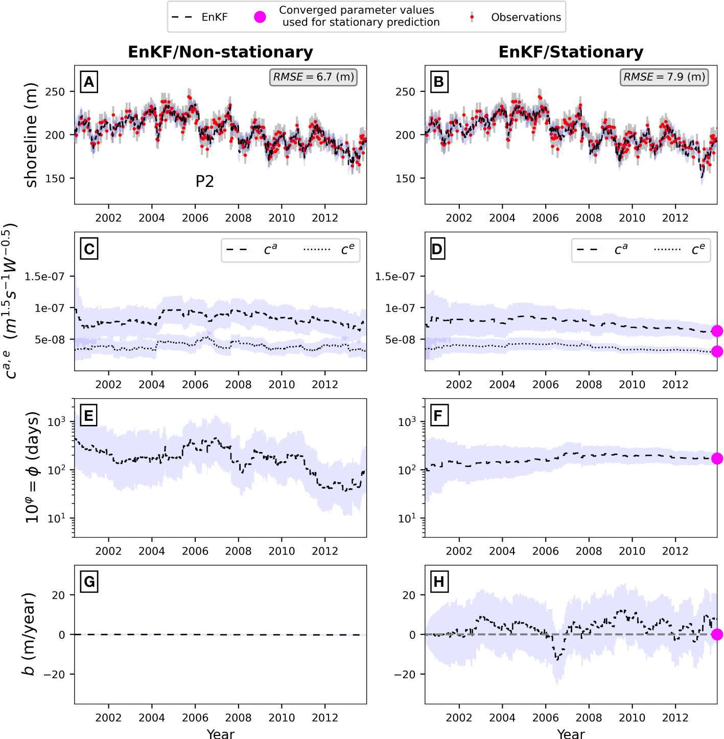
Figure 3 EnKF application to a multi-year (2000-2014) portion of the long-term dataset at the Gold Coast. Left and right panels show the non-stationary and stationary approaches, respectively. From top to bottom, each approach shows the shoreline observations and shoreline EnKF estimates (black line), c^a and c^e (dashed and dotted lines, respectively), ϕ = 10^φ and b. Blue bands indicate uncertainty, represented by the standard deviation of the ensemble (n=500). Magenta dots in the right panels indicate the converged parameters used for predicting shoreline time series with a stationary approach.

Applying the EnKF algorithm using the stationary parameter approach during the same 14-year time period is shown in the right panels of Figure 3. For both the non-stationary and stationary approaches, the EnKF produces a skillful shoreline hindcast because shoreline observations are available for data assimilation (Figures 3A, B). However, in contrast to the non-stationary EnKF results that assumed process-noise in the wave-driven parameters(c^a, c^e and ϕ), the stationary case that assumes negligible process-noise in these same three parameters results in c^a, c^e and ϕ (Figures 3D, F) varying more slowly as their uncertainty bands continuously reduce, leading to parameter convergence and approximately constant parameter magnitudes around ~2013. Additional model parameter contribution to the overall shoreline variability in this stationary approach is given by temporal variability in the residual term b (Figure 3H). The variability of this residual term compensates the minimal variability of the cross-shore driven parameters (c^a, c^e and ϕ, Figures 3D, F) and shows seasonal to interannual variability attributed to processes not resolved by the contribution of stationary cross-shore parameters. These unresolved processes contributed up to +/- 10 (m/year) of shoreline change at this site over this period.

The potential to physically relate the time-varying parameters of the nonstationary approach (Figures 3C, E, c^a, c^e and ϕ) to the underlying changes in wave forcing is now explored in the following section.

3.2 Correlation between estimated model parameters and wave climate covariates (Step 2)

Correlation analyses between non-stationary model parameters and wave climate covariates over the central 14-year time period (P2) are summarized in Figure 4. Panels A, B and C show the magnitude of the Pearson correlation coefficient (r, vertical axes) for c^a, c^e and φ, respectively. These include the correlation with the backwards running-average and standard deviation of Ω, H_s,b and $H_{s,b}^2$ (see colour lines in legend) at window lengths varying from 6 months to 10 years (horizontal axes). For c^a and c^e, the strongest negative and statistically significant correlations are given for the running-average dimensionless fall velocity at approximately 5-year time windows ($\overline{\text{Ω}}$, red continuous lines). Other wave climate covariates show similar but weaker correlation patterns. For the φ parameter (ϕ = 10^φ), all wave climate covariates show statistically significant and strong correlations for averaging windows larger than ~4-5 years. The existence of strong (|r| > 0.7) and statistically significant correlations enables the creation of linear parametrizations of c^a, c^e and φ as a function of the underlying physical changes in wave forcing.

FIGURE 4

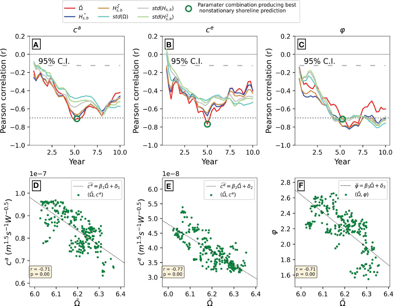
Figure 4 Summary results from Step 2 (Correlation analysis) and Step 3 (Parameterization) for each of the three wave-driven parameters (c^a, c^e and φ, left to right). Upper panels (A-C) show the Pearson correlation coefficient (vertical axes) for different wave climate covariates (coloured lines, see legend) at different averaging windows (horizontal axes). Horizontal and dotted black lines indicate the cut-off magnitude for strong correlations (|r|>0.7). Green open circles (panels a-c) indicate the time-window and wave climate covariate combination (here Ω at roughly ~5 years for all three parameters) resulting in the best shoreline prediction (using Equation 1) during the P2 period. Lower panels (D-F) show the data and linear parametrizations (Equation 3) resulting from the best non-stationary shoreline prediction.

3.3 Non-stationary parametrizations, model predictions and performance (Step 3-4)

Strong (|r| > 0.7) and significant (95% C.I.) correlations for different wave climate covariates and averaging windows resulted in 744 combinations of non-stationary $\widehat{c^a}$, $\widehat{c^e},\widehat{\phi }$ parameterizations (i.e., Equation 3) and an equivalent amount of modelled shoreline time series spanning the multi-decadal period. Figures 4D-F shows the linear parametrizations ($\widehat{c^a}$, $\widehat{c^e}$, $\widehat{\phi }$) of the combination that produced the optimal shoreline hindcast (minimum RMSE and maximum skill). All three linear expressions are derived from $\overline{\text{Ω}}$ averaged at a ~5-year running window (open green circles in Figures 4A-C). Figure 5 shows the shoreline model hindcast (green continuous line) corresponding to this combination of $\widehat{c^a}$, $\widehat{c^e}$, and $\widehat{\phi }$. Additionally, the shoreline model hindcast using a conventional stationary approach is shown in magenta using the converged values (magenta dots in Figure 3) and b = 0 for prediction purposes (e.g., Vitousek et al., 2017b). Setting b = 0 is also a reasonable assumption based on previous work that showed alongshore gradients in sediment transports are negligible at portion of the Gold Coast (Splinter et al., 2011) and neither the wave climate, nor the shoreline time series (see Figure 2) show a distinct long-term trend.

FIGURE 5

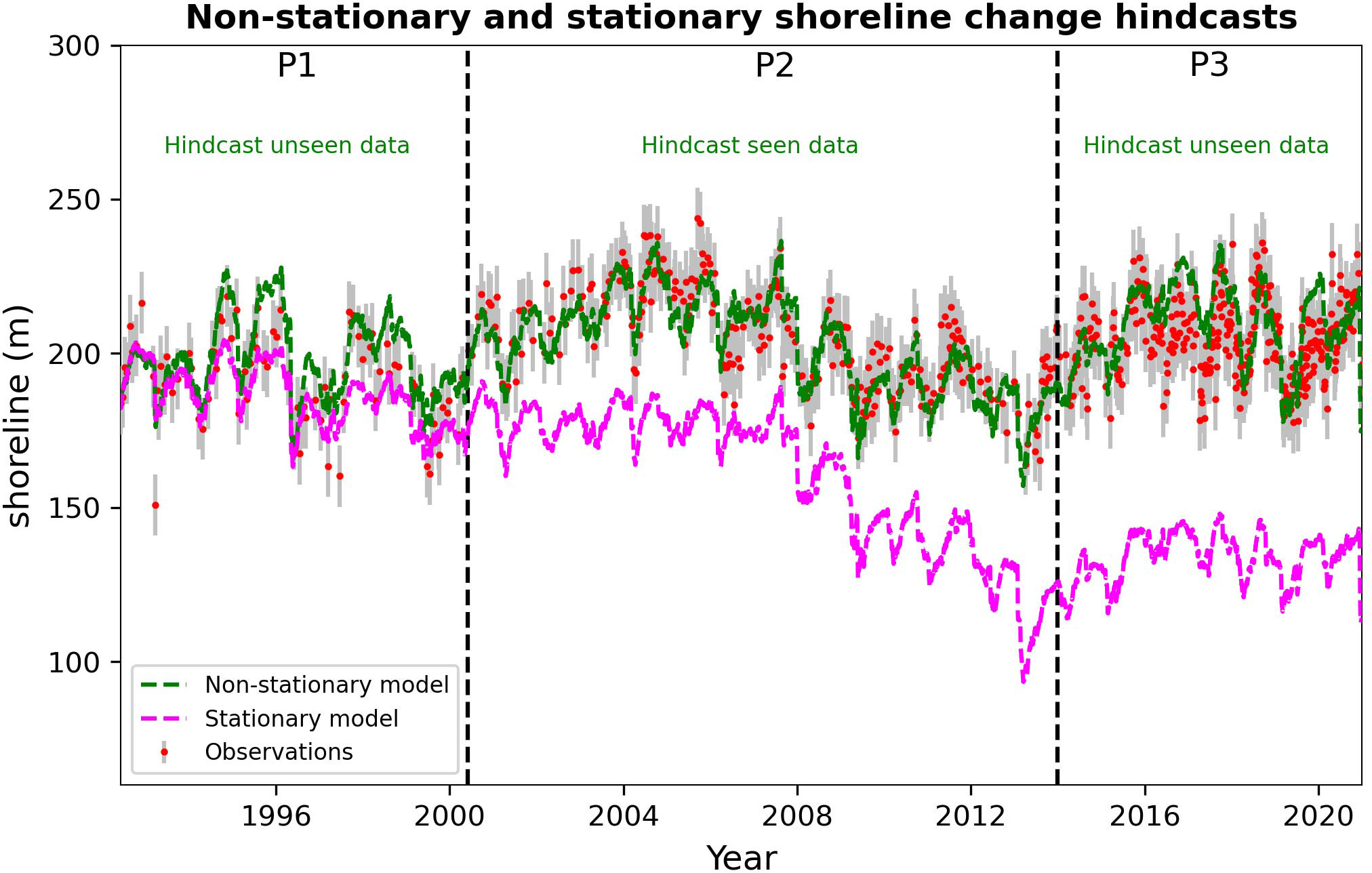
Figure 5 Comparison of shoreline predictions using non-stationary (green line) and stationary (magenta line) parameters with the ShoreFor model when b = 0. Both hindcasts were initialized from the same shoreline position in ~January 1992 and run forward in time using Equation 1.

Visual inspection of the prediction based on stationary model parameters exhibits a distinct long-term negative trend between 1992-2014 that accumulates in time despite setting b = 0. This suggests an overall long-term imbalance in the wave-driven cross-shore processes captured in the ShoreFor model using the stationary approach for model calibration. Encouragingly, the new non-stationary model that now enables model parameters to vary as a function of the underlying wave forcing, results in improved shoreline predictions over the full 28-year period, compared to the stationary approach (RMSE_{non-stationary} = 11.1 m; RMSE_stationary = 254.3 m). Performance statistics over the three different periods for both stationary and non-stationary approaches are summarized in Table 1. Notably, the RMSE magnitudes of the non-stationary prediction are on the order of the satellite-derived shorelines accuracy (~10-15 m) used to develop the non-stationary parametrizations, while the skill metric is strong (~>0.7) for all periods.

TABLE 1

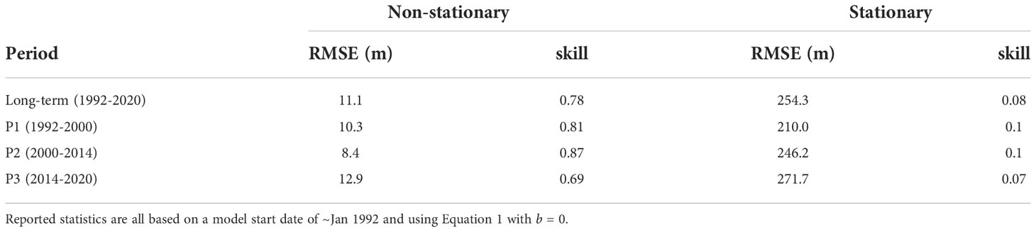
Table 1 Summary statistics of the stationary and non-stationary approaches for different time periods.

Of particular interest to this study, the non-stationary prediction is able to reproduce the long-term shoreline behaviour from seasonal to interannual time scales. Interestingly, post-2014 both the stationary and non-stationary approaches predict seasonal oscillations of the shoreline in the absence of any noticeable long-term trend. These results indicate a large difference in model performance and predicted shoreline evolution between both approaches at multi-decadal time scales, including the increasing divergence of the stationary model hindcasts at time scales greater than ~10 years.

4 Discussion

4.1 The non-stationary versus stationary approach

While the assumptions of using stationary parameters to model shoreline change may be valid for shorter-term prediction horizons of seasons to a few years (e.g., Splinter et al., 2013; Splinter et al., 2014; Davidson et al., 2017; D’Anna et al., 2020), the new results presented here demonstrate that improved shoreline predictions at decadal time scales can be achieved through the inclusion of non-stationary model parameters in the ShoreFor model. Provided a sufficiently high magnitude of parameter process-noise is defined, the non-stationary EnKF approach (Figure 3, left panels) allows for the time-varying estimation of model parameters (c^a, c^e, ϕ and b ~ 0) that best hindcasted the observed shoreline response. While this non-stationary approach has been embraced within the hydrological and water resources modelling communities in recent years (e.g., Milly et al., 2008; Pathiraja et al., 2018), it differs from previous Kalman Filter applications to shoreline modelling (e.g., Alvarez-Cuesta et al., 2021a,b; Long and Plant, 2012; Vitousek et al., 2017b; Vitousek et al., 2021) that assumed negligible magnitudes of process-noise to achieve time-invariant parameter convergence (e.g., stationary approach). While these previous Kalman Filter shoreline applications were based on the Yates et al. (2009) model rather than ShoreFor, both models follow the same underlying principles of wave driven equilibrium-based shoreline change and perform similarly from seasonal to interannual time frames (Castelle et al., 2014; Montaño et al., 2020; D’Anna et al., 2021). Although the ShoreFor model equilibrium formulation is determined from past wave conditions alone (Equation 2), the Yates et al. (2009) formulation depends on the shoreline observations seen during calibration to relate shoreline position to wave energy. The implication of these two assumptions is that ShoreFor shoreline predictions are sensitive to the wave forcing, whereas the Yates et al. (2009) approach tends to result in the modelled shorelines oscillating more persistently around the same long-term position irrespective of the underlying variability in wave forcing (D’Anna et al., 2021). This difference was also discussed by Vitousek et al. (2021), who analytically demonstrated that the ShoreFor model structure has a ‘perfect beach memory’, such that initial shoreline conditions and subsequent evolution are accumulated in time and ‘never forgotten’ (see Figure 5, magenta line). If b = 0, the stationary version of ShoreFor cannot produce a stable (i.e., zero-trend) shoreline hindcast in the absence of a balanced wave climate where erosive and accretive conditions equally contribute to the long-term shoreline behaviour. While both model assumptions are likely to have some merit in long-term equilibrium shoreline behaviour, the present work demonstrates that adjusting the ShoreFor model structure in response to the multi-year variability in wave forcing overcomes the issue of perfect beach memory and provides more realistic long-term predictions that are not as sensitive to a particular training period as is evident in the stationary approach (Figure 5).

Both the choice of model and calibration period become important when considering long-term shoreline predictions. Previous studies used stationary cross-shore parameters to explore future shoreline changes (Vitousek et al., 2017b; Alvarez-Cuesta et al., 2021b) without the inclusion of a residual term (b = 0). Using stationary model parameters, D’Anna et al. (2022) concluded that ShoreFor was sensitive to the chronology of the wave time series at various time scales. When examining the results from the Gold Coast, the stationary model hindcast reproduces the overall magnitude of seasonal and some interannual variability observed in the data, but what is most noticeable is an erroneous long-term erosional trend predicted between 1992-2014 before the model appears to stabilize and oscillate at a seasonal scale around a mean value between 2014-2020 (Figure 5). This clearly demonstrates the sensitivity of the model to variability and/or trends in the wave forcing and that a non-stationary version of ShoreFor can improve long-term shoreline predictions when future regional wave climates are expected to change.

4.2 Physical interpretation of model parameters

It is now of interest to physically interpret the observed (Step 1) and modelled (Steps 2 and 3) non-stationary parametrizations at the Gold Coast study site. Correlation analysis of six different wave climate covariates (mean and std of Ω, H_s,b and $H_{s,b}^2$) at different window lengths revealed strong correlations for the non-stationary parameters during P2 (Figure 4). Specifically, c^a and c^e, which were previously observed to co-vary proportionally (Figure 3C), showed strong negative correlations with $\overline{\text{Ω}}$ at 5-year running average windows. This negative relationship with $\overline{\text{Ω}}$ agrees with previous physical interpretations of these parameters as proxies for sediment transport efficiency (Splinter et al., 2014). Conceptually, this result implies that more/less energetic beach state systems ($\overline{\Omega }$) are less/more efficient (c^a and c^e) at transporting sediment between the surf zone and beach face. For instance, high-energy dissipative beach states typically have a deep offshore sand bar that rarely welds to the beach face. Lower-energy reflective beach states meanwhile are much more vulnerable to erosion and the sediment subsequently returns to the beach face during calmer periods (Phillips et al., 2017).

Interannual changes in waves and the intra-annual distribution of storminess (e.g., Splinter et al., 2017) may also influence the nearshore morphology (Price and Ruessink, 2011; Price and Ruessink, 2013) and net offshore bar migration events (Ruessink et al., 2009) at this site that all contribute to the observed shoreline dynamics. The observed co-variability and proportionality between c^a and c^e suggests that, in the absence of a residual term (b), multi-year changes in the wave forcing and the ShoreFor model parameters can reproduce the observed interannual shoreline variability (See Figure 5). However, over the longer-term spanning several decades, the integrated response of the slowly-varying wave climate produces a zero-trended shoreline response as discussed above.

The response parameter ϕ is used within the Shorefor model to low-pass filter the wave forcing to determine the equilibrium response (Equation 2). Incrementally increasing the response parameter for longer time periods has decreasing effect on the resulting filtered time series (see Figure 7 in Davidson et al., 2013). The response parameter ϕ, here represented by φ (ϕ = 10^φ) showed strong negative correlations with all wave climate covariates at averaging windows longer than ~4-5 years (Figure 4C). The less distinct peaks (or troughs) in correlation observed for φ compared to c^a and c^e are likely due to the more challenging estimation of this parameter by the EnKF due to the model insensitivity to small changes in ϕ for ϕ > 100 days as demonstrated in Ibaceta et al. (2020). Specifically, the combination of modelled $\widehat{c^a}$, $\widehat{c^e}$ and $\widehat{\phi }$ (Figures 4D-F) resulting in the best shoreline hindcast during the 14-year time period P2 (Figure 5) did not coincide with the maximum observed individual correlation for φ of approximately ~6 years. Instead, the best shoreline prediction occurred for the parametrization of $\widehat{\phi }$ as a function of the ~5-year averaged $\overline{\text{Ω}}$ (Figures 4A-C). Fortuitously, this 5-year window coincides with the minimum duration identified by Splinter et al. (2013) as optimal to calibrate the same shoreline numerical model used in this study for long-term hindcasts (> 5 years). To explore the negative relationship between $\overline{\text{Ω}}$ and ϕ in further detail, Figure 6 shows the multi-decadal (year to year) and intra-annual (summer and winter) distribution of storm events at the Gold Coast (bar chart, left axis), as well the estimated and modelled ϕ (right axis). In line with previous work exploring the links between ϕ and time scales of shoreline evolution (Splinter et al., 2017; Montaño et al., 2021; Schepper et al., 2021, Splinter et al., 2014), P2 (2000-2014) shows an initial period (~2000-2003) of few (<10), seasonally distributed storms and slow beach response (ϕ > 100 days). Then, the shoreline response shifts towards a more rapid shoreline behaviour (decreasing ϕ) coinciding with more storm events per year (>10, ~2005-2012) that are also more evenly distributed throughout individual years (e.g., Splinter et al., 2017). This increasing number of storm events coincides with slowly varying increases in $\overline{\text{Ω}}$ (Figure 2B) and match with the empirical negative relationship between $\overline{\text{Ω}}$ and ϕ, providing a physically-interpreted approach to adjust the shoreline model structure to periods of varying levels of storminess.

FIGURE 6

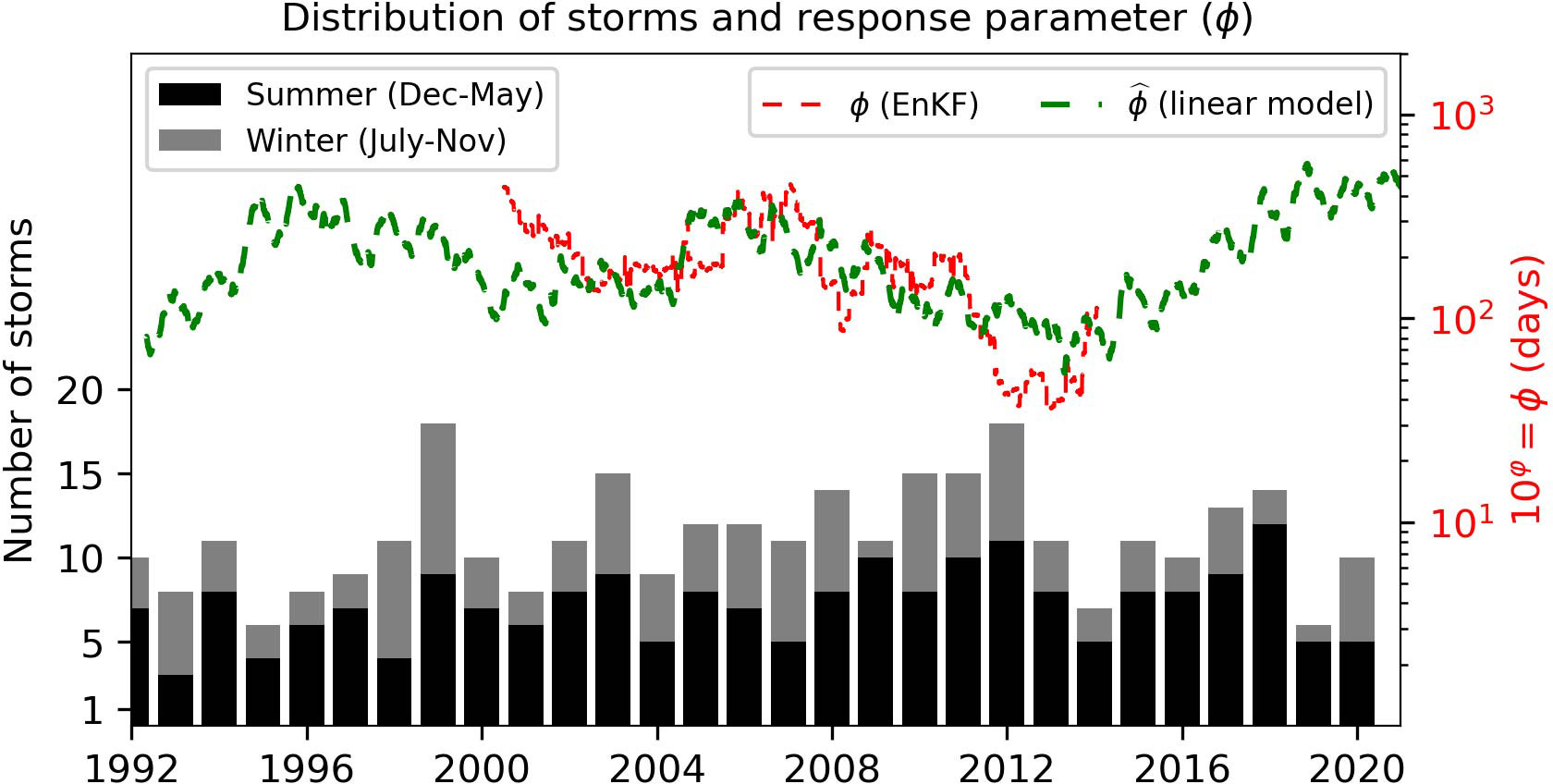
Figure 6 Bar chart and left axis: multi-decadal distribution of storm events per year and season (summer and winter). Storm events were obtained using a peak-over-threshold method over the long-term timeseries of significant wave height at the breaking position (i.e., H_s,b > H_95% and H_s,b > H_75% for at least 24 hours, Masselink et al., 2014). The green and red dashed lines (right axis) show the estimated (EnKF) and modelled magnitude of the ϕ parameter (pearson correlation with total number storms per year = -0.26, pvalue = 0.16).

5 Conclusions

This paper presents a new methodology for identifying and incorporating time-varying model parameters to predict shoreline response to changes in regional wave climate forcing, spanning seasonal to multi-year time periods of up to several decades. Extending on the Ensemble Kalman Filter technique developed by Ibaceta et al. (2020), new correlation analysis spanning a ~14-year period at the Gold Coast Australia study site, shows that all three cross-shore associated parameters of the ShoreFor model were negatively correlated with the mean dimensionless fall velocity, $\overline{\text{Ω},}$ at 5-year running average windows. By expressing this time-variability using simple linear regressions, an enhanced model that incorporates model parameter non-stationarity outperformed the predictions of a more conventional stationary approach over the 28-year period (see Figure 5).

Consistent with the conclusions of two recent review papers (Toimil et al., 2020; Splinter and Coco, 2021), the new analyses presented here demonstrate that adjusting the magnitude of time-varying model parameters at multi-year time scales can be interpreted as a physical adjustment of the shoreline response to changes in multi-year variability in the wave climate represented in the mathematical model structure. This may reduce the bias and uncertainty for future long-term shoreline predictions where the forcings associated with coastline change are expected to change (Morim et al., 2019; D’Anna et al., 2021). As suggested in D’Anna et al. (2022) the wider application of this methodology is now encouraged within different semi-empirical shoreline models and at a broad range of study sites that exhibit a range of differing wave and water level forcing, to further explore model adjustment to multi-year wave climate variability. It is realistic to anticipate that this can lead to the development of more generalized approaches (e.g., Splinter et al., 2014) to shoreline change modelling that are well suited to applications where time-variability of the model parameters is expected. By linking the magnitude of non-stationary model parameters to the underlying variability in wave forcing, this work presented the first effort to enhance multi-decadal shoreline predictions and provides an important step to achieve more reliable future shoreline projections in a changing wave climate.

Data availability statement

Wave data from the Gold Coast were provided by Gold Coast City Council (https://www.data.qld.gov.au/dataset/coastal‐data‐system‐waves‐gold‐coast). The CAWCR dataset was provided by CSIRO (http://hdl.handle.net/102.100.100/137152? index=1). Satellite data was provided by Kilian Vos from the Water Research Laboratory, UNSW (https://zenodo.org/record/4760145.Ypl3rKhByUk).

Author contributions

RI: conceptualization, methodology, modelling and analyses, writing, reviewing, and editing. KDS: supervision, conceptualization, methodology, writing, reviewing, and editing. MDH: supervision, conceptualization, reviewing and editing. ILT: supervision, conceptualization, reviewing and editing,

Acknowledgments

The authors acknowledge the Queensland Government and the City of Gold Coast for providing the wave buoy data. CSIRO is acknowledged for providing the CAWCR wave hindcast dataset. R.I. was funded by UNSW Faculty of Engineering, the Agencia Nacional de Investigación y Desarrollo (ANID, previously CONICYT), The Commonwealth of Australia through an Australian Government Research Training Program Scholarship and the NSW Environmental Trust Environmental Research Program (RD2015/0128). K.S. is the recipient of an Australian Research Council Australian Future Fellowship (project number FT220100009) funded by the Australian Government.

Conflict of interest

The authors declare that the research was conducted in the absence of any commercial or financial relationships that could be construed as a potential conflict of interest.

Publisher’s note

All claims expressed in this article are solely those of the authors and do not necessarily represent those of their affiliated organizations, or those of the publisher, the editors and the reviewers. Any product that may be evaluated in this article, or claim that may be made by its manufacturer, is not guaranteed or endorsed by the publisher.

References

Almeida L. P., Efraim de Oliveira I., Lyra R., Scaranto Dazzi R. L., Martins V. G., Henrique da Fontoura Klein A. (2021). Coastal analyst system from space imagery engine (CASSIE): Shoreline management module. Environ. Model. Software 140, 105033. doi: 10.1016/j.envsoft.2021.105033

CrossRef Full Text | Google Scholar

Alvarez-Cuesta M., Toimil A., Losada I. J. (2021a). Modelling long-term shoreline evolution in highly anthropized coastal areas . part 1 : Model description and validation. Coast. Eng. 169, 103960. doi: 10.1016/j.coastaleng.2021.103960

CrossRef Full Text | Google Scholar

Alvarez-Cuesta M., Toimil A., Losada I. J. (2021b). Modelling long-term shoreline evolution in highly anthropized coastal areas . part 2 : Assessing the response to climate change. Coast. Eng. 168, 103961. doi: 10.1016/j.coastaleng.2021.103961

CrossRef Full Text | Google Scholar

Barnard P. L., Short A. D., Harley M. D., Splinter K. D., Vitousek S., Turner I. L., et al. (2015). Coastal vulnerability across the pacific dominated by El Niño/Southern oscillation. Nat. Geosci. 8, 801–807. doi: 10.1038/ngeo2539

CrossRef Full Text | Google Scholar

Black K., Mead S. (2001). Design of the gold coast reef for surfing, public amenity and coastal protection: Surfing aspects. J. Coast. Res. 29, 115–130. http://www.jstor.org/stable/25736210

Google Scholar

Boak L., McGrath J., Jackson L A. (2000). “IENCE ? a case Study ? the northern gold coast beach protection strategy,” in Coast. Eng. 2000, Proceedings. ASCE. doi: 10.1061/40549(276)289

CrossRef Full Text | Google Scholar

Castelle B., Marieu V., Bujan S., Ferreira S., Parisot J. P., Capo S., et al. (2014). Equilibrium shoreline modelling of a high-energy meso-macrotidal multiple-barred beach. Mar. Geol. 347, 85–94. doi: 10.1016/j.margeo.2013.11.003

CrossRef Full Text | Google Scholar

Castelle B., Masselink G., Scott T., Stokes C., Konstantinou A., Marieu V., et al. (2021). Satellite-derived shoreline detection at a high-energy meso-macrotidal beach. Geomorphology 383, 107707. doi: 10.1016/j.geomorph.2021.107707

CrossRef Full Text | Google Scholar

D’Anna M., Castelle B., Idier D., Rohmer J., Le Cozannet G., Thieblemont R., et al. (2021). Uncertainties in shoreline projections to 2100 at truc vert beach (France): Role of Sea-level rise and equilibrium model assumptions. J. Geophys. Res. Earth Surf. 126, e2021JF006160. doi: 10.1029/2021JF006160

CrossRef Full Text | Google Scholar

D’Anna M., Idier D., Castelle B., Le Cozannet G., Rohmer J., Robinet A. (2020). Impact of model free parameters and sea-level rise uncertainties on 20-years shoreline hindcast: the case of truc vert beach (SW France). Earth Surf. Process. Landforms. 45, 1895–1907. doi: 10.1002/esp.4854

CrossRef Full Text | Google Scholar

D’Anna M., Idier D., Castelle B., Rohmer J., Cagigal L., Mendez F. J. (2022). Effects of stochastic wave forcing on probabilistic equilibrium shoreline response across the 21st century including sea-level rise. Coast. Eng. 175, 104149. doi: 10.1016/j.coastaleng.2022.104149

CrossRef Full Text | Google Scholar

Davidson M. A., Splinter K. D., Turner I. L. (2013). A simple equilibrium model for predicting shoreline change. Coast. Eng. 73, 191–202. doi: 10.1016/j.coastaleng.2012.11.002

CrossRef Full Text | Google Scholar

Davidson M. A., Turner I. L. (2009). A behavioral template beach profile model for predicting seasonal to interannual shoreline evolution. J. Geophys. Res. Earth Surf. 114. doi: 10.1029/2007JF000888

CrossRef Full Text | Google Scholar

Davidson M. A., Turner I. L., Splinter K. D., Harley M. D. (2017). Annual prediction of shoreline erosion and subsequent recovery. Coast. Eng. 130, 14–25. doi: 10.1016/j.coastaleng.2017.09.008

CrossRef Full Text | Google Scholar

Deng C., Liu P., Wang W., Shao Q., Wang D. (2019). Modelling time-variant parameters of a two-parameter monthly water balance model. J. Hydrol. 573, 918–936. doi: 10.1016/j.jhydrol.2019.04.027

CrossRef Full Text | Google Scholar

Durrant T., Greenslade D., Hemer M., Trenham C. (2014). A global wave hindcast focused on the central and South Pacific (Technical Report No. 070). The Centre for Australian Weather and Climate Research. https://www.cawcr.gov.au/technical-reports/CTR_070.pdf

Google Scholar

Evensen G. (2009). Data assimilation: The ensemble kalman filter. 2nd ed (Heidelberg: Springer Berlin). doi: 10.1007/978-3-540-38301-7

CrossRef Full Text | Google Scholar

Hemer M. A., Zieger S., Durrant T., O’Grady J., Hoeke R. K., McInnes K. L., et al. (2017). A revised assessment of australia’s national wave energy resource. Renew. Energy 114, 85–107. doi: 10.1016/j.renene.2016.08.039

CrossRef Full Text | Google Scholar

Ibaceta R., Splinter K. D., Harley M. D., Turner I. L. (2020). Enhanced coastal shoreline modelling using an ensemble kalman filter to include non-stationarity in future wave climates. Geophys. Res. Lett. 47, e2020GL090724. doi: 10.1029/2020GL090724

CrossRef Full Text | Google Scholar

Jackson D., Short A. (2020). “1 - introduction to beach morphodynamics,” in Sandy beach morphodynamics. Eds. Jackson D. W. T., Short A. D. (Elsevier), 1–14. doi: 10.1016/B978-0-08-102927-5.00001-1

CrossRef Full Text | Google Scholar

Jaramillo C., González M., Medina R., Turki I. (2021). An equilibrium-based shoreline rotation model. Coast. Eng. 163, 103789. doi: 10.1016/j.coastaleng.2020.103789

CrossRef Full Text | Google Scholar

Jaramillo C., Jara M. S., González M., Medina R. (2020). A shoreline evolution model considering the temporal variability of the beach profile sediment volume (sediment gain / loss). Coast. Eng. 156, 103612. doi: 10.1016/j.coastaleng.2019.103612

CrossRef Full Text | Google Scholar

Kalman R. E. (1960). A new approach to linear filtering and prediction problems. Trans. ASME–Journal Basic Eng. 82, 35–45. doi: 10.1115/1.3662552

CrossRef Full Text | Google Scholar

Kroon A., de Schipper M. A., van Gelder P.H.A.J.M., Aarninkhof S. G. J. (2020). Ranking uncertainty: Wave climate variability versus model uncertainty in probabilistic assessment of coastline change. Coast. Eng. 158, 103673. doi: 10.1016/j.coastaleng.2020.103673

CrossRef Full Text | Google Scholar

Le Cozannet G., Bulteau T., Castelle B., Ranasinghe R., Wöppelmann G., Rohmer J., et al. (2019). Quantifying uncertainties of sandy shoreline change projections as sea level rises. Sci. Rep. 9, 42. doi: 10.1038/s41598-018-37017-4

PubMed Abstract | CrossRef Full Text | Google Scholar

Le Cozannet G., Oliveros C., Castelle B., Garcin M., Idier D., Pedreros R., et al. (2016). Uncertainties in sandy shorelines evolution under the bruun rule assumption. Front. Mar. Sci. 3. doi: 10.3389/fmars.2016.00049

CrossRef Full Text | Google Scholar

Long J. W., Plant N. G. (2012). Extended kalman filter framework for forecasting shoreline evolution. Geophys. Res. Lett. 39, L13603. doi: 10.1029/2012GL052180

CrossRef Full Text | Google Scholar

Ludka B. C., Guza R. T., O’Reilly W. C., Yates M. L. (2015). Field evidence of beach profile evolution toward equilibrium. J. Geophys. Res. Ocean. 120, 7574–7597. doi: 10.1002/2015JC010893

CrossRef Full Text | Google Scholar

Luijendijk A., Hagenaars G., Ranasinghe R., Baart F., Donchyts G., Aarninkhof S. (2018). The state of the world’s beaches. Sci. Rep. 8, 1–11. doi: 10.1038/s41598-018-24630-6

PubMed Abstract | CrossRef Full Text | Google Scholar

Masselink G., Austin M., Scott T., Poate T., Russell P. (2014). Role of wave forcing, storms and NAO in outer bar dynamics on a high-energy, macro-tidal beach. Geomorphology 226, 76–93. doi: 10.1016/j.geomorph.2014.07.025

CrossRef Full Text | Google Scholar

Miller J. K., Dean R. G. (2004). A simple new shoreline change model. Coast. Eng. 51, 531–556. doi: 10.1016/j.coastaleng.2004.05.006

CrossRef Full Text | Google Scholar

Milly P. C. D., Betancourt J., Falkenmark M., Hirsch R. M., Kundzewicz Z. W., Lettenmaier D. P., et al. (2008). Climate change: Stationarity is dead: Whither water management? Sci. (80-. ). 319, 573–574. doi: 10.1126/science.1151915

CrossRef Full Text | Google Scholar

Montaño J., Coco G., Antolínez J. A. A., Beuzen T., Bryan K. R., Cagigal L., et al. (2020). Blind testing of shoreline evolution models. Sci. Rep. 10, 1–10. doi: 10.1038/s41598-020-59018-y

PubMed Abstract | CrossRef Full Text | Google Scholar

Montaño J., Coco G., Cagigal L., Mendez F., Rueda A., Bryan K. R., et al. (2021). A multiscale approach to shoreline prediction. Geophys. Res. Lett. 48, 1–11. doi: 10.1029/2020gl090587

CrossRef Full Text | Google Scholar

Morim J., Hemer M., Wang X. L., Cartwright N., Trenham C., Semedo A., et al. (2019). Robustness and uncertainties in global multivariate wind-wave climate projections. Nat. Clim. Change 9, 711–718. doi: 10.1038/s41558-019-0542-5

CrossRef Full Text | Google Scholar

Muir F., Hurst M., Vitousek S., Hansom J., Rennie A., Fitton J., et al. (2020). “Predicting coastal change in Scotland across decadal-centennial timescales using a process-driven one-line model,” in Coastal Management 2019. 551–563. doi: 10.1680/cm.65147.551

CrossRef Full Text | Google Scholar

Odériz I., Mori N., Shimura T., Webb A., Silva R., Mortlock T. R. (2022). Transitional wave climate regions on continental and polar coasts in a warming world. Nat. Clim. Change 12, 662–671. doi: 10.1038/s41558-022-01389-3

CrossRef Full Text | Google Scholar

Pathiraja S., Anghileri D., Burlando P., Sharma A., Marshall L., Moradkhani H. (2018). Time-varying parameter models for catchments with land use change: The importance of model structure. Hydrol. Earth Syst. Sci. 22, 2903–2919. doi: 10.5194/hess-22-2903-2018

CrossRef Full Text | Google Scholar

Pathiraja S., Marshall L., Sharma A., Moradkhani H. (2016a). Hydrologic modeling in dynamic catchments: A data assimilation approach. Water Resour. Res. 52, 3350–3372. doi: 10.1002/2015WR017192

CrossRef Full Text | Google Scholar

Pathiraja S., Marshall L., Sharma A., Moradkhani H. (2016b). Detecting non-stationary hydrologic model parameters in a paired catchment system using data assimilation. Adv. Water Resour. 94, 103–119. doi: 10.1016/j.advwatres.2016.04.021

CrossRef Full Text | Google Scholar

Phillips M. S., Harley M. D., Turner I. L., Splinter K. D., Cox R. J. (2017). Shoreline recovery on wave-dominated sandy coastlines: the role of sandbar morphodynamics and nearshore wave parameters. Mar. Geol. 385, 146–159. doi: 10.1016/j.margeo.2017.01.005

CrossRef Full Text | Google Scholar

Phinn S. R., Hastings P. A. (1995). Southern oscillation influences on the gold coast’s summer wave climate. J. Coast. Res. 11, 946–958. http://www.jstor.org/stable/4298394

Google Scholar

Price T. D., Ruessink B. G. (2011). State dynamics of a double sandbar system. Cont. Shelf Res. 31, 659–674. doi: 10.1016/j.csr.2010.12.018

CrossRef Full Text | Google Scholar

Price T. D., Ruessink B. G. (2013). Observations and conceptual modelling of morphological coupling in a double sandbar system. Earth Surf. Process. Landforms 38, 477–489. doi: 10.1002/esp.3293

CrossRef Full Text | Google Scholar

Ranasinghe R. (2016). Assessing climate change impacts on open sandy coasts: A review. Earth-Science Rev. 160, 320–332. doi: 10.1016/j.earscirev.2016.07.011

CrossRef Full Text | Google Scholar

Ranasinghe R. (2020). On the need for a new generation of coastal change models for the 21 st century. Sci. Rep. 10, 2010. doi: 10.1038/s41598-020-58376-x

PubMed Abstract | CrossRef Full Text | Google Scholar

Roelvink D., Huisman B., Elghandour A., Ghonim M. (2020). Efficient modeling of complex sandy coastal evolution at monthly to century time scales. Front. Mar. Sci. 7, 1–20. doi: 10.3389/fmars.2020.00535

PubMed Abstract | CrossRef Full Text | Google Scholar

Ruessink B. G., Pape L., Turner I. L. (2009). Daily to interannual cross-shore sandbar migration: Observations from a multiple sandbar system. Cont. Shelf Res. 29, 1663–1677. doi: 10.1016/j.csr.2009.05.011

CrossRef Full Text | Google Scholar

Schepper R., Almar R., Bergsma E. W. J., de Vries S., Reniers A., Davidson M. A., et al. (2021). Modelling cross-shore shoreline change on multiple timescales and their interactions. J. Geophys. Res. Earth Surf. 9(6), 582. doi: 10.3390/jmse9060582

CrossRef Full Text | Google Scholar

Short A. D. (2022). Australian Beach systems: Are they at risk to climate change? Ocean Coast. Manage. 224, 106180. doi: 10.1016/j.ocecoaman.2022.106180

CrossRef Full Text | Google Scholar

Splinter K. D., Coco G. (2021). Challenges and opportunities in coastal shoreline prediction. Front. Mar. Sci. 8. doi: 10.3389/fmars.2021.788657

CrossRef Full Text | Google Scholar

Splinter K. D., Strauss D. R., Tomlinson R. B. (2011). Assessment of post-storm recovery of beaches using video imaging techniques: A case study at gold coast, Australia. IEEE Trans. Geosci. Remote Sens. 49, 4704–4716. doi: 10.1109/TGRS.2011.2136351

CrossRef Full Text | Google Scholar

Splinter K. D., Turner I. L., Davidson M. A. (2013). How much data is enough? the importance of morphological sampling interval and duration for calibration of empirical shoreline models. Coast. Eng. 77, 14–27. doi: 10.1016/j.coastaleng.2013.02.009

CrossRef Full Text | Google Scholar

Splinter K. D., Turner I. L., Davidson M. A., Barnard P., Castelle B., Oltman-Shay J. (2014). A generalized equilibrium model for predicting daily to inter-annual shoreline response. J. Geophys. Res. Earth Surf. 119, 1936–1958. doi: 10.1002/2014JF003106

CrossRef Full Text | Google Scholar

Splinter K. D., Turner I. L., Reinhardt M., Ruessink G. (2017). Rapid adjustment of shoreline behavior to changing seasonality of storms: observations and modelling at an open-coast beach. Earth Surf. Process. Landforms 42, 1186–1194. doi: 10.1002/esp.4088

CrossRef Full Text | Google Scholar

Toimil A., Camus P., Losada I. J., Alvarez-Cuesta M. (2021). Visualising the uncertainty cascade in multi-ensemble probabilistic coastal erosion projections. Front. Mar. Sci. 202, 103110. doi: 10.3389/fmars.2021.683535

CrossRef Full Text | Google Scholar

Toimil A., Camus P., Losada I. J., Le Cozannet G., Nicholls R. J., Idier D., et al. (2020). Climate change-driven coastal erosion modelling in temperate sandy beaches: Methods and uncertainty treatment. Earth-Science Rev., 202, 103110. doi: 10.1016/J.EARSCIREV.2020.103110

CrossRef Full Text | Google Scholar

Toimil A., Losada I. J., Camus P., Díaz-simal P. (2017). Managing coastal erosion under climate change at the regional scale. Coast. Eng. 128, 106–122. doi: 10.1016/j.coastaleng.2017.08.004

CrossRef Full Text | Google Scholar

Turner I. L. (2006). Discriminating modes of shoreline response to offshore-detached structures. J. Waterw. Port Coastal Ocean Eng. 132, 180–191. doi: 10.1061/(ASCE)0733-950X

CrossRef Full Text | Google Scholar

van Enckevort I. M. J., Ruessink B. G., Coco G., Suzuki K., Turner I. L., Plant N. G., et al. (2004). Observations of nearshore crescentic sandbars. J. Geophys. Res. Ocean. 109, 1–17. doi: 10.1029/2003JC002214

CrossRef Full Text | Google Scholar

Vitousek S., Barnard P. L., Limber P. (2017a). Can beaches survive climate change? J. Geophys. Res. Earth Surf. 122, 1060–1067. doi: 10.1002/2017JF004308

CrossRef Full Text | Google Scholar

Vitousek S., Barnard P. L., Limber P., Erikson L., Cole B. (2017b). A model integrating longshore and cross-shore processes for predicting long-term shoreline response to climate change. J. Geophys. Res. Earth Surf. 122, 782–806. doi: 10.1002/2016JF004065

CrossRef Full Text | Google Scholar

Vitousek S., Cagigal L., Montaño J., Rueda A., Mendez F., Coco G., et al. (2021). The application of ensemble wave forcing to quantify uncertainty of shoreline change predictions. J. Geophys. Res. Earth Surf. 126, e2019JF005506. doi: 10.1029/2019jf005506

CrossRef Full Text | Google Scholar

Vos K., Harley M. D., Splinter K. D., Simmons J. A., Turner I. L. (2019a). Sub-Annual to multi-decadal shoreline variability from publicly available satellite imagery. Coast. Eng. 150, 160–174. doi: 10.1016/j.coastaleng.2019.04.004

CrossRef Full Text | Google Scholar

Vos K., Harley M. D., Splinter K. D., Walker A., Turner I. L. (2020). Beach slopes from satellite-derived shorelines. Geophys. Res. Lett. 47, e2020GL088365. doi: 10.1029/2020GL088365

CrossRef Full Text | Google Scholar

Vos K., Harley M., Turner I. (2021). Large Regional variability in coastal erosion caused by ENSO. 1–16. doi: 10.21203/rs.3.rs-666160/v1

CrossRef Full Text | Google Scholar

Vos K., Splinter K. D., Harley M. D., Simmons J. A., Turner I. L. (2019b). CoastSat: A Google earth engine-enabled Python toolkit to extract shorelines from publicly available satellite imagery. Environ. Model. Software 122, 104528. doi: 10.1016/j.envsoft.2019.104528

CrossRef Full Text | Google Scholar

Vousdoukas M. I., Ranasinghe R., Mentaschi L., Plomaritis T. A., Athanasiou P., Luijendijk A., et al. (2020). Sandy coastlines under threat of erosion. Nat. Clim. Change 10, 260–263. doi: 10.1038/s41558-020-0697-0

CrossRef Full Text | Google Scholar

Westra S., Thyer M., Leonard M., Kavetski D., Lambert M. (2014). A strategy for diagnosing and interpreting hydrological model nonstationarity. Water Resour. Res. 50, 5090–5113. doi: 10.1002/2013WR014719

CrossRef Full Text | Google Scholar

Wong P. P., Losada I. J., Gatusso J. P., Hinkel J., A K., McInnes K. L., et al. (2014). “Coastal systems and low-lying areas,” in Climate change 2014 – impacts, adaptation and vulnerability: Part a: Global and sectoral aspects: Working group II contribution to the IPCC fifth assessment report: Volume 1: Global and sectoral aspects. Ed. Intergovernmental Panel on Climate Change (Cambridge: Cambridge University Press), 361–410. doi: 10.1017/CBO9781107415379.010

CrossRef Full Text | Google Scholar

Wright L. D., Short A. D. (1984). Morphodynamic variability of surf zones and beaches: A synthesis. Mar. Geol. 56, 93–118. doi: 10.1016/0025-3227(84)90008-2

CrossRef Full Text | Google Scholar

Wright L. D., Short A. D., Green M. O. (1985). Short-term changes in the morphodynamic states of beaches and surf zones: An empirical predictive model. Mar. Geol. 62, 339–364. doi: 10.1016/0025-3227(85)90123-9

CrossRef Full Text | Google Scholar

Xiong M., Liu P., Cheng L., Deng C., Gui Z., Zhang X., et al. (2019). Identifying time-varying hydrological model parameters to improve simulation efficiency by the ensemble kalman filter: A joint assimilation of streamflow and actual evapotranspiration. J. Hydrol. 568, 758–768. doi: 10.1016/j.jhydrol.2018.11.038

CrossRef Full Text | Google Scholar

Yates M. L., Guza R. T., O’Reilly W. C. (2009). Equilibrium shoreline response: Observations and modeling. J. Geophys. Res. Ocean. 114, C09014. doi: 10.1029/2009JC005359

CrossRef Full Text | Google Scholar

Yates M. L., Guza R. T., O’Reilly W. C., Hansen J. E., Barnard P. L. (2011). Equilibrium shoreline response of a high wave energy beach. J. Geophys. Res. Ocean. 116, 1–13. doi: 10.1029/2010JC006681

CrossRef Full Text | Google Scholar

Zarifsanayei A. R., Antolínez J. A. A., Etemad-Shahidi A., Cartwright N., Strauss D. (2022). A multi-model ensemble to investigate uncertainty in the estimation of wave-driven longshore sediment transport patterns along a non-straight coastline. Coast. Eng. 173, 104080. doi: 10.1016/j.coastaleng.2022.104080

CrossRef Full Text | Google Scholar

Zeng L., Xiong L., Liu D., Chen J., Kim J. S. (2019). Improving parameter transferability of GR4J model under changing environments considering nonstationarity. Water (Switzerland) 11(10), 2029. doi: 10.3390/w11102029

CrossRef Full Text | Google Scholar