 Samuel Sainz-Villegas
 Camino Fernández de la Hoz
 José A. Juanes
 Araceli Puente
- IHCantabria - Instituto de Hidráulica Ambiental de la Universidad de Cantabria, Santander, Spain
Modelling non-native marine species distributions is still a challenging activity. This study aims to predict the global distribution of five widespread introduced seaweed species by focusing on two mains aspects of the ensemble modeling process: (1) Does the enforcement of less complex models (in terms of number of predictors) help in obtaining better predictions? (2) What are the implications of tuning the configuration of individual algorithms in terms of ecological realism? Regarding the first aspect, two datasets with different number of predictors were created. Regarding the second aspect, four algorithms and three configurations were tested. Models were evaluated using common evaluation metrics (AUC, TSS, Boyce index and TSS-derived sensitivity) and ecological realism. Finally, a stepwise procedure for model selection was applied to build the ensembles. Models trained with the large predictor dataset generally performed better than models trained with the reduced dataset, but with some exceptions. Regarding algorithms and configurations, Random Forest (RF) and Generalized Boosting Models (GBM) scored the highest metric values in average, even though, RF response curves were the most unrealistic and non-smooth and GBM showed overfitting for some species. Generalized Linear Models (GLM) and MAXENT, despite their lower scores, fitted smoother curves (especially at intermediate complexity levels). Reliable and biologically meaningful predictions were achieved. Inspecting the number of predictors to include in final ensembles and the selection of algorithms and its complexity have been demonstrated to be crucial for this purpose. Additionally, we highlight the importance of combining quantitative (based on multiple evaluation metrics) and qualitative (based on ecological realism) methods for selecting optimal configurations.
1 Introduction
The number of marine seaweeds outside their natural boundaries has increased in the last decades generating impacts on biodiversity and economy (Schaffelke et al., 2006). This makes the development of management tools necessary, where species distribution models (SDMs) play a crucial role. SDMs can help in the early detection of invasions and predict the extent of the potential spread (Marcelino and Verbruggen, 2015; Martínez et al., 2015). However, modelling non-native marine species distributions is still challenging in terms of model building, evaluation and selection.
Characterization of marine species distributions is often dependent on the quality of the data. In general, logistical and economic constraints in the sampling process result in records of low spatial resolution that are biased towards the most important economic or conservation areas (Robinson et al., 2011). Furthermore, many of these species are undergoing range shifts during the colonization process. These shifts generate two important issues in the correlative methods used to model species distributions: (1) the model assumption that species records reflect stable relationships with the environment is violated, and (2) environmental combinations outside the range of variables included in the model-building process may lead to inaccurate results (Elith et al., 2010; Lake et al., 2020). In recent years, different approaches have been developed in order to deal with these issues. Most of them focused their efforts on a few topics such as the reduction of sampling bias, the choice of environmental predictors or the analysis of algorithm settings.
Previous research suggests that one of the most effective techniques to mitigate sampling bias (the bias generated due to unequal sampling efforts) is the downsampling of occurrence records by thinning or reducing the number of records in areas with higher densities (Fourcade et al., 2014; Lake et al., 2020). While reducing sampling bias has been demonstrated to improve the quality of the predictions, no consensus among researchers can be found for the other issues (Sequeira et al., 2018). For example, the question about the number and the kind of predictors that should be included in species distribution models remains still unclear. It seems that large predictor datasets lead to more complex models which may overfit the data while simpler models often improve transferability (Petitpierre et al., 2017; Sequeira et al., 2018). However, there is not a single best method for identifying and choosing the optimal subset of biologically-relevant predictors, which makes necessary the exploration of different configurations.
Another important issue is the selection of the statistical algorithm among the increasing number of modelling techniques. MAXENT (Phillips et al., 2006) is the most widely used as its good performance has been proven in a wide variety of species. Other modelling techniques such as Boosted Regression Trees (BRT: Friedman, 2001), Generalized Linear Models (GLM: McCullagh and Nelder, 1983) or Random Forest (RF: Breiman, 2001) are also frequently used for predicting marine species distributions (Melo-Merino et al., 2020). However, modelling outputs for a single species tend to be heterogeneous among algorithms. This suggests that there is not a best single algorithm as each of them has its own weaknesses and strengths [for review see Franklin (2010); Peterson et al. (2011); Guisan et al. (2017)]. One of the methodological approaches proposed to address this issue consists in aggregating the outputs from different algorithms into a single ensemble model (Thuiller, 2004; Araújo and New, 2007). While there is a large body of information concerning ensemble modelling for terrestrial plants (Hao et al., 2019), less information can be found relative to marine seaweeds, where most of the research is focused on individual algorithms (Marcelino and Verbruggen, 2015). In general terms, these ensemble approaches have been suggested to reduce uncertainty in predictions and increase model’s accuracy (Marmion et al., 2009; Thuiller et al., 2019), although some exceptions exist (Zhu and Peterson, 2017; Hao et al., 2020).
Ensemble models should be carefully constructed and evaluated to avoid unrealistic distributions. The analysis of different configuration settings (also known as model tuning or model parameterization) for each algorithm is a key aspect for this purpose (Elith et al., 2010). Several authors have explored this part of the model building process suggesting that there is not a best single criterion for selecting the best configuration. In fact, it seems to be species-specific (Anderson and Gonzalez, 2011; Hallgren et al., 2019). Again, according to literature, MAXENT configuration is the most explored (e.g. Merow et al., 2013; Phillips et al., 2017). It has been demonstrated that the algorithm is very sensitive to different combinations of model features, regularization multiplier and maximum number of iterations (Morales et al., 2017; Valavi et al., 2022). The other algorithms mentioned before have received less attention, but some examples of model tuning recommendations can be found in the literature. For example, Elith et al. (2008) developed a working guide for BRTs and Hallgren et al. (2017); Hallgren et al. (2019) tested the sensitivity of GLMs, RFs, BRTs and seven more algorithms to different configurations. Despite the evidence on how important is the process of model tuning, to our knowledge, no examples exploring individual algorithm configurations in ensemble models for non-indigenous seaweeds can be found in the literature.
This study aims to predict the global distribution of five widespread introduced seaweed species using an ensemble model approach and focusing on two issues of the model building process: (1) Does the enforcement of less complex models (in terms of number of predictors) help in obtaining better predictions? (2) What are the implications of tuning the configuration of individual algorithms in terms of ecological realism?
2 Materials and methods
2.1 Data
2.1.1 Species data
This study was focused on five introduced seaweeds: Asparagopsis armata, Bonnemaisonia hamifera, Rugulopteryx okamurae, Sargassum muticum and Undaria pinnatifida. For detailed information on species’ ecology, introduction history and native or invasive ranges see (Supplementary Material S1 Table S.1.1). Biological records were collected from the Global Biodiversity Information Facility (GBIF, 2021), the Macroalgal Herbarium Portal (MHE, 2021) and the Ocean Biodiversity Information System (OBIS, 2021). Only records with geographic information were considered, including records updated until January 2020. For R. okamurae, as few non-duplicated presence points were detected in the non-native region, a literature review was done in order to complement this lack of points (a total of 6 points were added in Europe and 39 points were removed from Australia and New Zealand due to misidentifications). Every record was carefully inspected to remove possible geographical errors. Finally, datasets were downsampled in order to reduce sampling bias and to avoid duplicated records using the R package “spThin” (Aiello-Lammens et al., 2015) with a thinning distance of 10km. This approach also guaranteed only one record per grid cell. Figure 1 shows the geographical distribution of records from the global and native ranges. True absences were unavailable, so 10,000 pseudo-absences were generated randomly in the geographic space. Presence and pseudo-absences were weighted equally (prevalence = 0.5) (Barbet-Massin et al., 2012). All models were fitted using both native and non-native presence records.
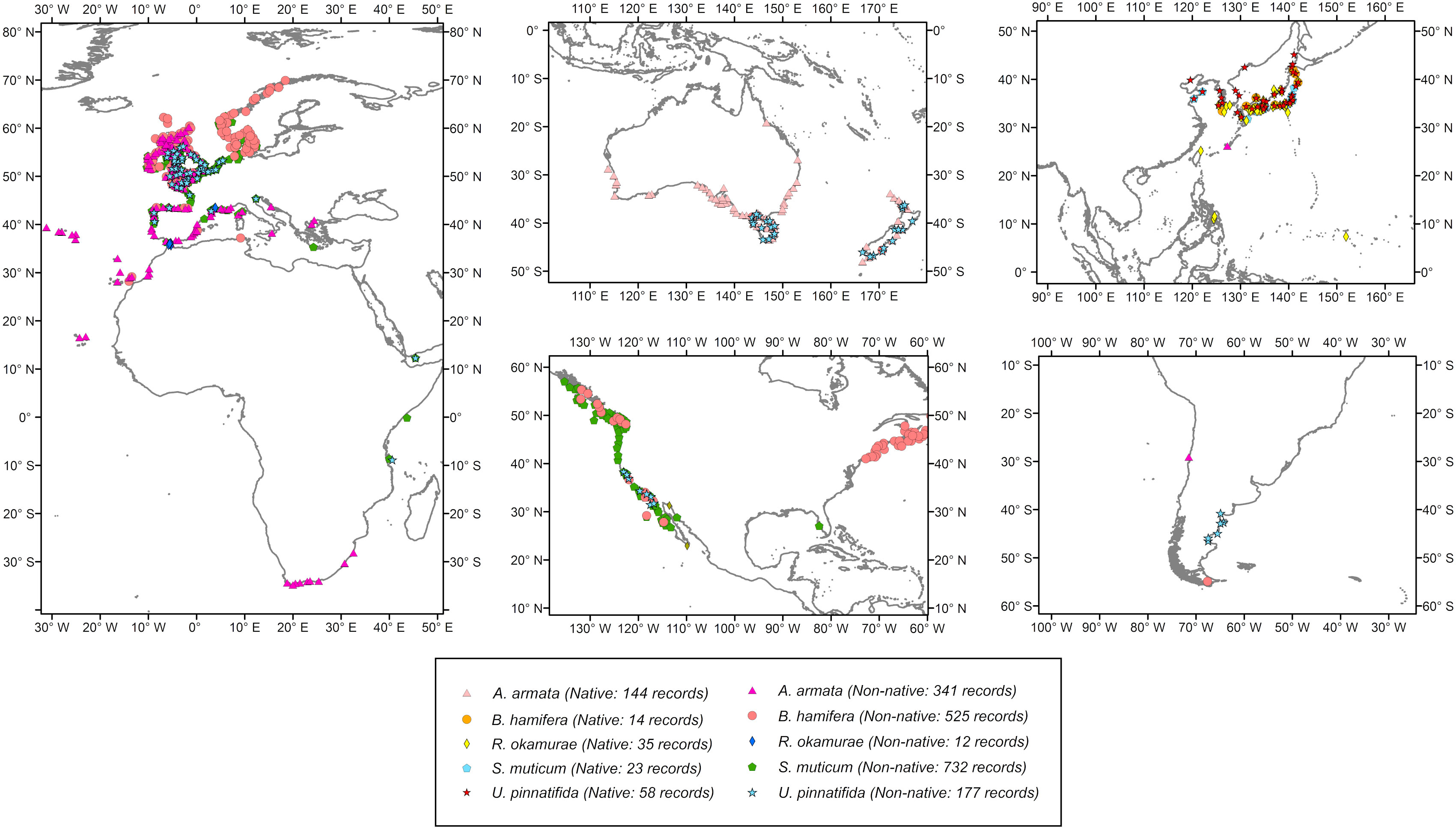
Figure 1 Geographical distribution and final number of presence records (after filtering and downsampling) both for the native and invaded regions. A. armata: Asparagopsis armata, B. hamifera: Bonnemaisonia hamifera, R. okamurae: Rugulopteryx okamurae, S. muticum: Sargassum muticum and U. pinnatifida: Undaria pinnatifida.
2.1.2 Environmental data
Environmental predictor variables were obtained from the BIO-ORACLE 2.0 database (Assis et al., 2018) with a spatial resolution of 5 arc-min (approximately 9.2 km grid cells at the equator) and global extent. Among the predictors available, a first selection was made collecting those variables most frequently incorporated in seaweeds SDMs studies (Martínez et al., 2012; Marcelino and Verbruggen, 2015). This resulted in a preliminary dataset of 13 environmental predictors: Sea Surface Temperature Range (SSTR), Mean Sea Surface Temperature (SSTM), Maximum Sea Surface Temperature (SSTMax), Minimum Sea Surface Temperature (SSTMin), Salinity (Sal), Phosphate (Ps), Nitrates (Nit), Mean Cloud Cover fraction (Cl), Mean Photosynthetic Active Radiation (PARM), Max Photosynthetic Active Radiation (PARMax), Mean chlorophyll A concentration (Chl-A), Dissolved oxygen (OD), Diffuse attenuation coefficient at 490 nm (DAC) (see Table S1.2 in Supplementary Material 1 for descriptions). Grid cells deeper than 70m were excluded for each environmental layer using the GEBCO bathymetry (GEBCO Bathymetric Compilation Group, 2020), as they were considered to be outside the potential habitat for these macroalgae species.
2.2 Experimental design
The experimental approach proposed in this study had the primary goal of finding the best configuration for ensemble modeling of the five introduced seaweeds distributions. To do so, two aspects that affect the quality of the predictions were explored following the structure shown in Figure 2.- Predictors Selection
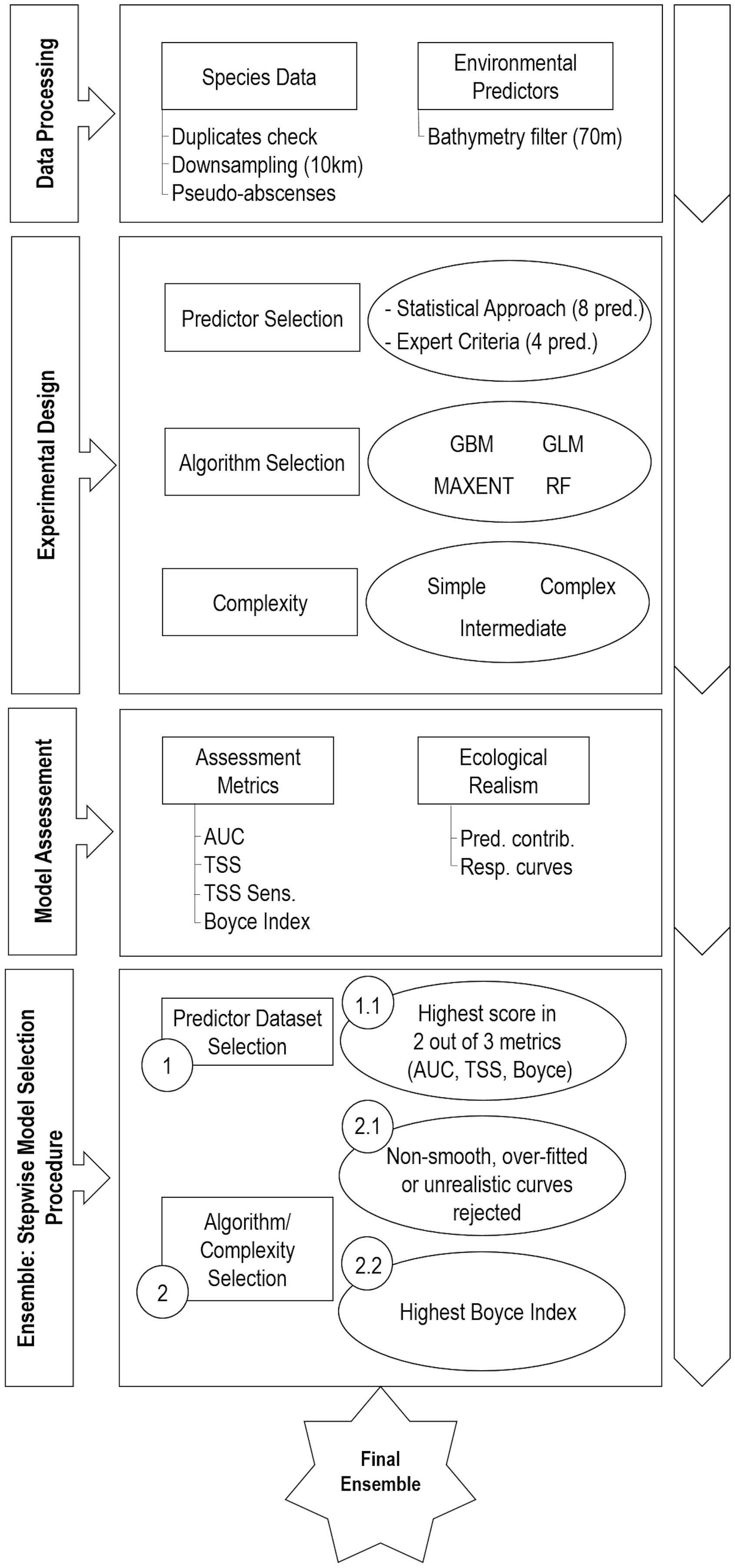
Figure 2 Experimental design and work flow for predicting the global distribution of the five introduced seaweed in an ensemble modeling approach. AUC, area under the receiver–operating curve; Pred. contrib., Predictor contribution; pred., Predictors; Resp. curves, Response curves; TSS Sens., TSS-derived sensitivity; TSS, true skill statistic.
o Number of predictors (2 Levels): (1) Statistical Approach, (2) Expert Criteria- Algorithm Selection and Parameterization
o Algorithms (4 Levels): (1) RF, (2) MAXENT, (3) GLM, (4) GBM
o Parameterization Complexity (3 Levels): (1) Simple, (2) Intermediate, (3) Complex
2.2.1 Predictor selection
Predictor preliminary data were combined in two datasets containing different number of predictors. Two different criteria were applied: (1) Large dataset: Predictors selected using a statistical approach based on a Pearson’s correlation coefficient ≤0.70 and variable inflation factor ≤10. From each correlated pair of variables, only one was kept for further analysis (that showing the lower VIF). From non-correlated variables, only those with a VIF ≤10 were kept in a stepwise process. In each step, the variable with the highest VIF was removed and then, the index was recalculated. The process is repeated until every variable scored a VIF index lower than 10 (de la Hoz et al., 2019b); (2) Reduced dataset: Predictors selected using an expert-criteria approach supported on general knowledge on the physiology and ecology of seaweeds (according to Lüning et al., 1990). Dataset 1 use eight (SSTR, SSTM, Sal, Ps, Nit, Cl, PARM, Chl-A) and dataset 2 use four (SSTR, SSTM, Sal, PARM) environmental layers respectively.
2.2.2 Algorithm selection and parameterization
Four SDM algorithms were fitted for each of the previously defined datasets with a simple, intermediate and complex parametrization by tuning default configurations. A regression technique (generalized linear model (GLM)) and three machine learning approaches (two tree‐based techniques: random forest (RF) and Boosted Regression Trees (BRT); and MAXENT) were selected for analysis. All the algorithms were implemented in the R software (version 3.6.2; R Core Team, 2020) using the package “BIOMOD2” (version 3.4.6; Thuiller et al., 2009).
Different settings of the parameters mainly involved in model complexity (see Merow et al., 2014) were explored. For GLMs, model complexity levels were achieved by adjusting the flexibility of the response curves. Simple GLMs were fitted considering only linear terms, intermediate GLMs also considered second order polynomials and for complex GLMs, polynomials greater than second order were added. Interactions between predictors were not considered for any level of complexity. For tree-based algorithms, different configurations of the maximum number of trees were considered. Simple, intermediate, and complex RF models were built by setting the maximum number of trees in 100, 250 and 500 respectively. For BRTs, the number of trees was set in 1000, 2500 and 5000. Finally, complexity levels in MAXENT were defined by allowing different combinations of model features: only linear for the simplest model, linear and quadratic for the intermediate model and linear, quadratic and hinge for the complex model. Rest of parameters were set to default in order to simplify the experimental design.
2.2.3 Model assessment
Individual models’ performance was assessed using an internal validation approach which consisted in randomly splitting the species dataset (75% of occurrence records used for training and 25% for evaluation) five times. Each model was evaluated using the area under the receiver operating characteristic curve (AUC) (Hanley and McNeil, 1982), the true skill statistic (TSS) (Allouche et al., 2006) and TSS-derived sensitivity calculated with the threshold that optimized TSS scores (Thuiller et al., 2009). AUC values vary from 0.5 to 1. Model predictions are considered “very good” for AUC values over 0.9, “reasonable predictions” for values between 0.7 and 0.9, and “poorly accurate” for values below 0.7 (Araújo and Pearson, 2005). TSS values oscillate from 0 to 1. The predictive power of models (in terms of TSS) is classified as “poor” for values < 0.4, “good” in the range 0.4–0.8 and “excellent” from 0.8 to 1 (Zhang et al., 2015). Additionally, the Boyce index was calculated in order to compare probabilistic predictions to presence-only observations (Boyce et al., 2002). This metric gets values between -1 and +1, with positive values indicating predictions consistent with the presences’ distributions, negative values indicating low quality predictions and values near zero indicating predictions not different from random models (Hirzel et al., 2006). All metrics were calculated using “BIOMOD2” and “ecospat” (version 3.1; Di Cola et al., 2017) packages in R software. Model performance differences between models trained with each predictor dataset were tested using a Wilcoxon signed-rank test (WSRT), as previously implemented in Verbruggen et al. (2013). Additionally, the algorithm-complexity effects on model performance were tested using non-parametric, rank-based multivariate methods implemented in the “nparMD” package (version 0.1.0; Kiefel and Bathke, 2020) using the R software. Statistical details of the underlying methodology can be found in Bathke and Harrar (2016) and in Munzel and Brunner (2000). Post-hoc analysis was conducted using a paired two-tailed Wilcoxon signed-rank test for pairwise comparisons when significant effects were detected. Overfitting was assessed quantitatively and qualitatively. The former was assessed by comparing threshold-dependent omission rates with theoretically levels of omission. To do so, the 10th percentile presence threshold rule was applied to the training data to convert the continuous prediction to a binary prediction. Then, the omission rates were estimated using the test data. Overfitting was detected if calculated rates exceeded approximately the 10 percent of omission (Radosavljevic and Anderson, 2014). This analysis was carried out using the same training-testing data subsets previously created for evaluation. Qualitatively, overfitting was assessed by visually inspecting the response curves and the distribution maps.
2.3 Model selection process for final ensemble predictions
Final ensemble structure was selected using a stepwise approach. First, the effect of predictors selection on the predictive power of models was evaluated. For this purpose, the values of the three metrics (AUC, TSS and Boyce) for each combination of algorithm/parameterization-complexity were averaged across species datasets. The combination of predictors receiving the lowest score on average was discarded for further analysis. Finally, the selection of the algorithms included in the final ensemble model and its parametrization was decided by checking the values of the metrics, and by inspecting the response curves generated and the contribution of each environmental variable. Models with AUC<0.9 or TSS<0.8 were automatically discarded for further analysis. For the remaining, models with non-smooth curves, over-fitted or unrealistic curves were also discarded, retaining only one configuration (the most realistic) for the final ensemble. If response curves were consistently unrealistic across every configuration for one algorithm, the entire algorithm was discarded for the final ensemble. On the other hand, when two or more configurations led to similar realistic curves, the model with the highest performance [in terms of Boyce Index as it is the most appropriate when working with presence-only information (Di Cola et al., 2017)] was selected. Final ensembles of individual models were constructed for each species using the “Weighted Average” technique already implemented in “BIOMOD2” package.
3 Results
3.1 Model configuration implications for model performance
3.1.1 Predictor dataset
In general terms, model performance could be considered very good according to AUC and TSS averaged cross-validation evaluation scores (AUC>0.9 and TSS>0.8) for all species and predictor dataset, except for R. okamurae models trained with the larger predictor dataset. These models scored an average value below 0.8 for TSS (Table 1). Presence-only metric Boyce-Index showed predictions with average values over 0.7 in all cases. Sensitivity could also be considered good for all species and datasets, with more than 90% of presences well predicted, although thresholds were set considerably low (<0.35).
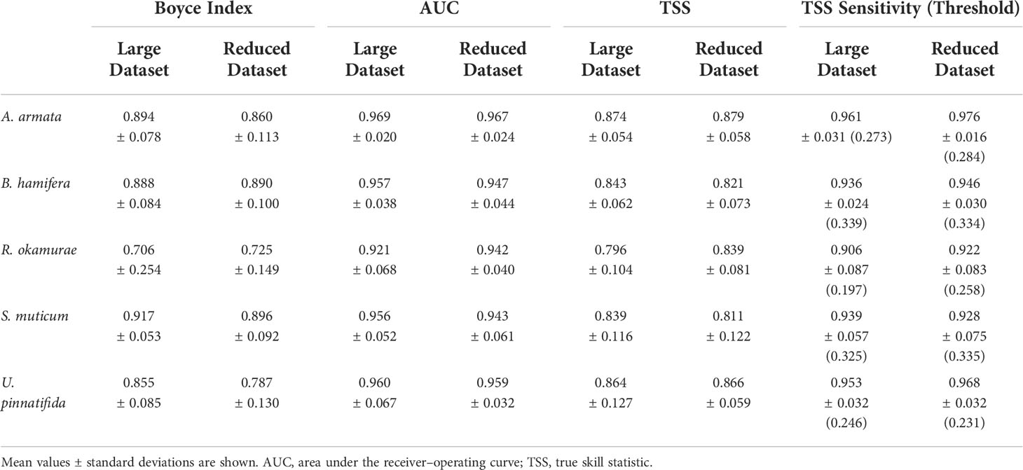
Table 1 Summary of model assessment metrics (Boyce Index, AUC, TSS and TSS Sensitivity + Threshold (in brackets)) for the Large Dataset (8 predictors) and the Reduced Dataset (4 predictors).
For four out of five species, models performed significantly better [according to WSRT test, p-values<0.05; Table S1.3 in (Supplementary Material 1)] when trained with the large predictor dataset for at least two of the three metrics considered. R. okamurae was the only species performing better on the Reduced dataset (across the three metrics considered), although differences were exclusively significant for AUC (p=0.007; Table S1.3 in Supplementary Material 1).
3.1.2 Algorithms and parameterization
Both algorithms and parameterization have shown a high significant effect on model performance for all species and datasets, except for R. okamurae. For this species, the algorithm and parameterization effects were significant for models trained with the large predictor dataset, but only the algorithm effect was significant for models trained with the Reduced predictor dataset (Table S1.4 in Supplementary Material 1). RF and GBM model performance were higher on average than GLM and MAXENT (in terms of AUC and TSS) for each species and predictor dataset (Figure 3, Tables S1.5 and S1.6 in Supplementary Material 1). No clear patterns could be discerned from the Boyce index metric. Pairwise comparisons showed that these differences were not consistently significant across complexity levels, datasets and species (Tables S1.7 and S1.8 in Supplementary Material 1).
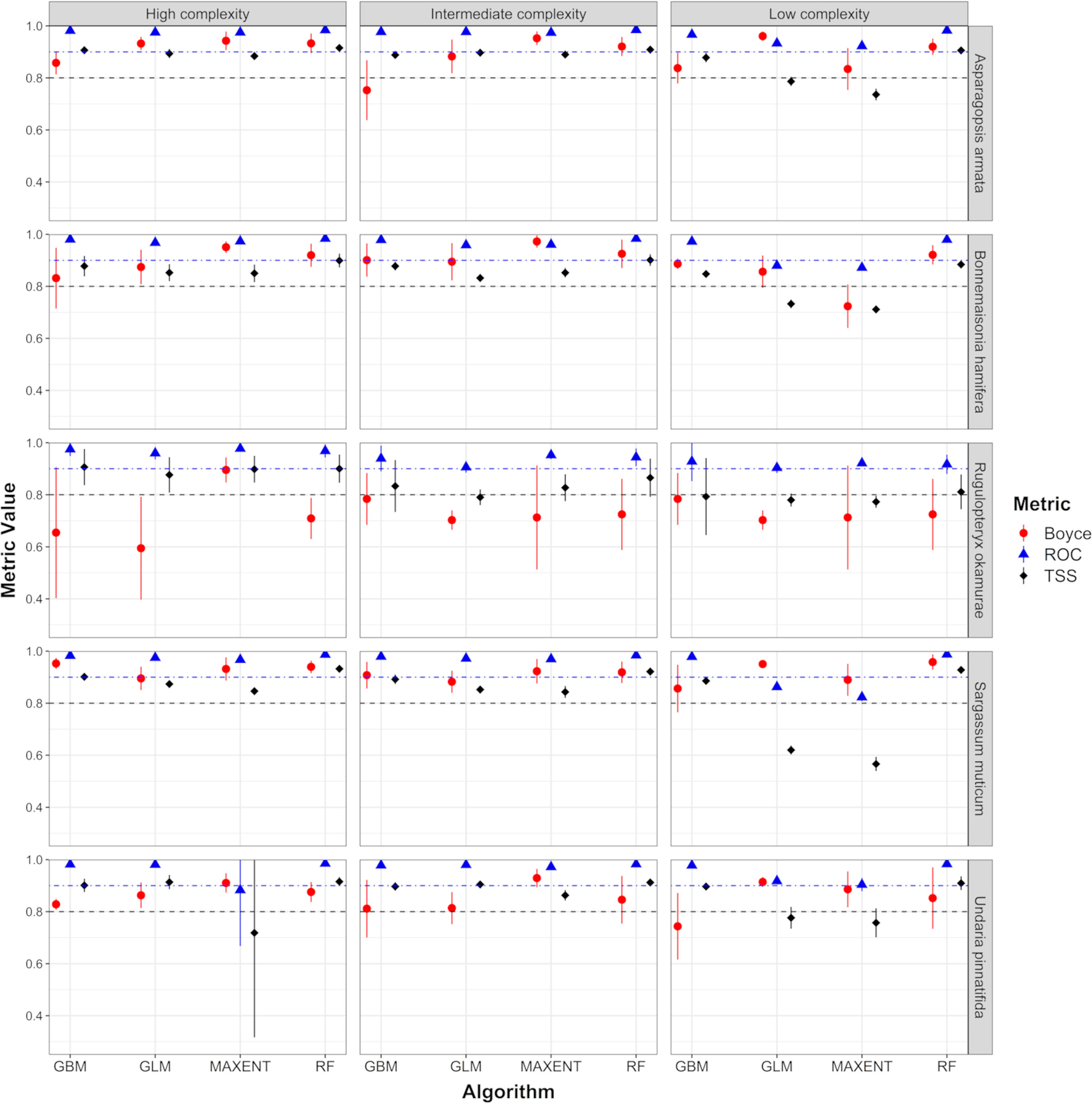
Figure 3 Model performance (in terms of Boyce Index, AUC and TSS) for each species and algorithm + complexity configuration. Results shown in this figure correspond to models trained using the large predictor dataset, excluding R. okamurae results, which correspond to models trained using the reduced predictor dataset. Dashed lines represent the thresholds applied for model selection in section 2.3 (Blue – AUC threshold = 0.9; Black – TSS threshold = 0.8). AUC, area under the receiver–operating curve; BRT, Boosted Regression Trees; GBM, Generalized Linear Models; RF, Random Forest; TSS, true skill statistic.
Complexity levels explored by different algorithm parameterizations had different effects on model performance depending on the algorithm considered (Figures 3, S1.1). Pairwise comparisons (paired two-tailed Wilcoxon signed-rank test) showed that GLM and MAXENT models tuned with an intermediate or high complexity outperform simpler models for the whole group of species and predictor datasets (in terms of TSS and AUC), with the exception of R. okamurae. In these cases, high complexity models performed significantly better than intermediate complexity models for B. hamifera and S. muticum (only MAXENT). On the contrary, RF models did not show significant differences between complexity levels. Comparisons between levels for GBM models did not identify clear patterns. GBM models trained with the large dataset and intermediate and high complexity levels outperformed simpler models (in terms of AUC and TSS) only for A. armata and B. hamifera. When these models were trained with the reduced dataset, they also outperformed simpler models (but only in terms of AUC) for S. muticum and U. pinnatifida (Tables S1.9 and S1.10 in Supplementary Material 1).
3.2 Model configuration implications in terms of ecological realism
Two aspects were considered as indicators when analyzing whether models behaved in a biologically meaningful way: (1) Response curves fitted for each environmental variable (Figures S1.2 and S1.3 in Supplementary Material 1) and (2) Variable contributions. According to the former, it was noticed that RF models fitted the most unrealistic and non-smooth curves from the pool of algorithms considered. For this algorithm, discrimination between suitable and unsuitable conditions was not clear with few differences between complexity levels (see Figure 4). Additionally, habitat suitability values were always bellow 0.75, even in areas with high density of presences. Smooth bell-shaped responses for well-known parameters such as SSTM were not identified for this algorithm in any of the species analyzed. MAXENT and GLM performance, in terms of the quality of their response curves, was similar for every species considered. As expected, simpler models (limited to linear terms) only captured partial responses for parameters which follow unimodal responses. Models fitted with an intermediate level of complexity (allowing for Linear and Quadratic terms in MAXENT and second order polynomial in GLMs) showed the smoothest and most realistic curves as they represent close approximations of physiological thresholds for some predictors such as SSTM or PARM (an example for S. muticum is provided in Figure 4). R. okamurae GLM models fitted with an intermediate level of complexity were the exception as non-consistent curves were achieved among replicates. Forcing these two algorithms to higher levels of complexity increase the overfitting rate for those models (see Figure 5) and, in some cases, led to non-consistent predictions among replicates (e.g. A. armata, B. hamifera or R. okamurae). GBM curves smoothness was similar for each complexity level but intermediate or complex models led, in general, to better results. For some species, such as A. armata, R. okamurae or U. pinnatifida, signs of overfitting could be detected, more noticeably in higher complexity levels (Figure 5).
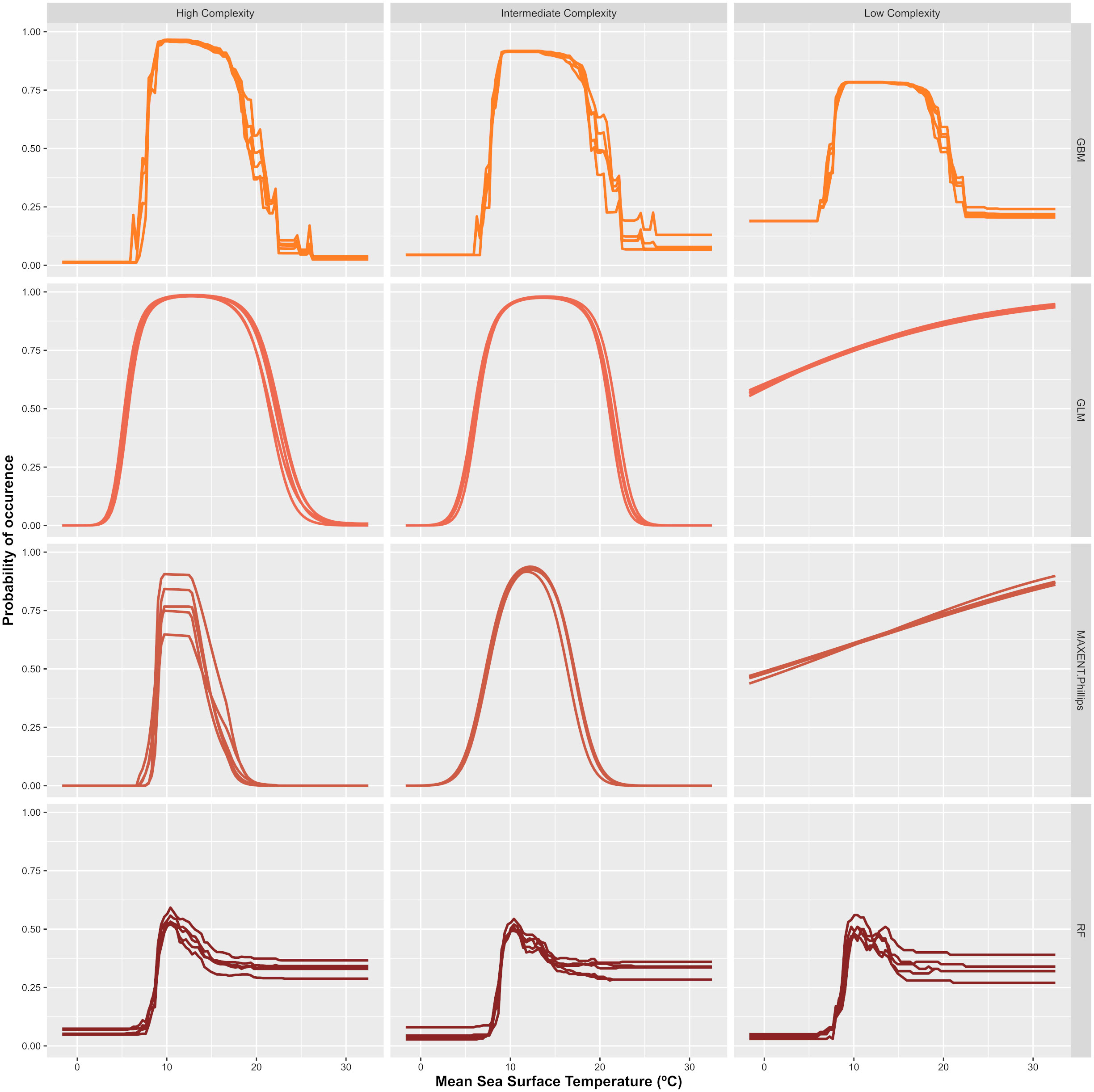
Figure 4 Example of the Mean Sea Surface Temperature response curves generated for Sargassum muticum with the different algorithms and complexity configurations. The x-axes represents the Mean Sea Surface Temperature (SSTM: °C) and the y-axes the probability of occurrence (from 0 to 1).
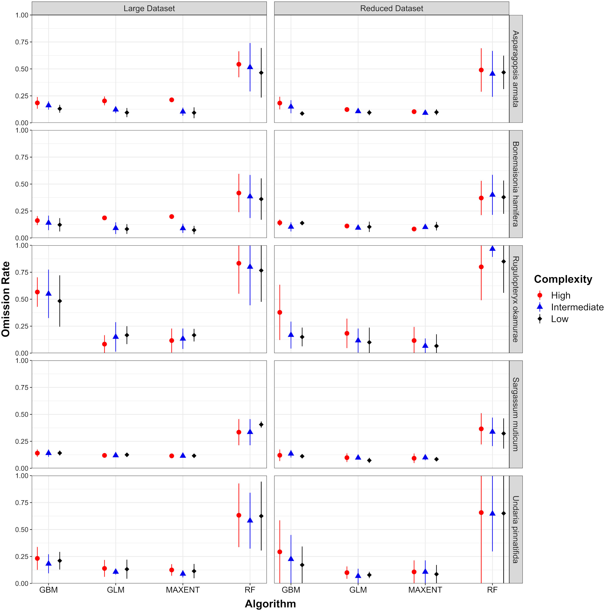
Figure 5 Omission rates obtained for each species and each combination of algorithm, complexity configuration and environmental dataset using the 10th percentile presence threshold. Omission rates higher than the theoretical expectation (in this case 0.1) indicate overfitting.
Concerning environmental variable contributions, MAXENT and GLM models fitted with an intermediate or high level of complexity identified SSTM as the most important variable (Tables S1.11 and S1.12, 13 in Supplementary Material 1), as expected when modelling global ranges. Simpler models identified other predictors such as SSTR, PARM or salinity as the most important predictors. GBM models consistently identified SSTM as the variable with the highest contribution in each complexity level. RF discrimination power was lower. This resulted in predictors such as SSTM, SSTR, PARM and Salinity having similar contributions.
3.3 Model selection and final ensemble distributions
Models included in the final ensemble for each species were selected following the selection process proposed in section 2.3 (see Supplementary Material 2 for details). A. armata and B. hamifera ensembles were constructed by fitting GLMs and MAXENT models with an intermediate level of complexity. S. muticum and U. pinnatifida ensembles also incorporated GLMs, MAXENT and GBM models fitted with the higher level of complexity. Finally, R. okamurae ensembles were build using GBM and MAXENT models fitted with an intermediate level of complexity. All models were built using the 8-predictors dataset with the exception of R. okamurae (built with the 4-predictors dataset) (see Figure 6 and Supplementary Material 2 for details).
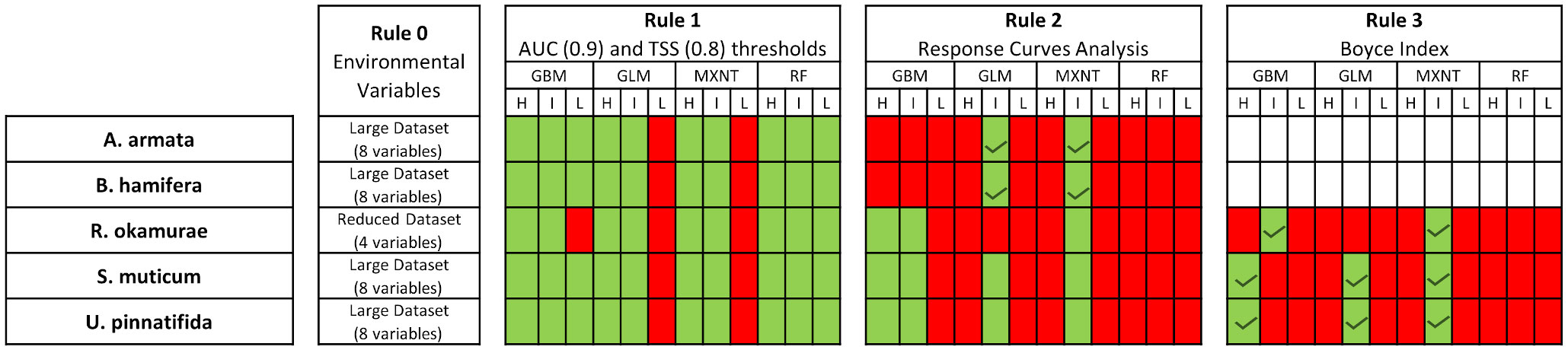
Figure 6 Results for the selection process proposed in section 2.3 to select the final configuration of ensemble models. Red colored squares represent algorithms and configurations discarded for further analysis in each step of the process. Green colors represent the configurations kept for further analysis in each step until only one configuration was kept per algorithm. Green ticks represent the final algorithms and configurations used to build the final ensembles. H, High complexity; I, Intermediate complexity; L, Low Complexity; BRT, Boosted Regression Trees; GBM, Generalized Linear Models; RF, Random Forest; MXNT, MAXENT.
Final ensemble model’s performance was considered very good for the whole group of species according to AUC and TSS, with values over 0.97 and 0.83 respectively (Table S1.13 in Supplementary Material 1). Boyce index values were close to perfect predictions (values over 0.9) for A. armata, B. hamifera, S. muticum and U. pinnatifida. R. okamurae’s Boyce index also identified high quality predictions, but the value was lower (0.77). TSS sensitivity showed values over 90% of presences well-predicted (with thresholds established over a 0.33 value of habitat suitability) for all species, except for R. okamurae in which sensitivity fell to 60% due to the high threshold considered (close to a 0.7 value of habitat suitability).
Finally, ensemble models were evaluated by qualitative visual examination, based on expert knowledge about these species’ current distributions. Overall, geographic patterns shown in Figure 7 matched well with current species range, both in their native and non-native regions. A. armata modelled distribution (Figure 7A) is well defined by its temperate origins, with some regions out of its known range identified as highly suitable. This is the case of the south-eastern and south-western coasts of South America. Other temperate introduced species, such as S. muticum and U. pinnatifida have already reached those areas. This pattern was well captured by its ensemble model. In the Mediterranean Sea, A. armata modelled distribution identified intermediate to high suitability areas in both the north (European coasts) and the south coasts (African coasts). S. muticum and U. pinnatifida ensembles (Figures 7D, 7E) identified those areas with low to intermediate habitat suitability values (with some exceptions such as the Thau Lagoon in France), particularly in the northern coasts of Africa. According to the habitat suitability values (Figure 7B), B. hamifera southern distribution limit in Europe is clearly established in Portugal, with some exceptions in the Mediterranean Sea. Instead, its northern limits were identified at higher latitudes if compared with the other temperate species. R. okamurae non-native range (Figure 7C) was identified by high suitability values in southern Europe, Brazil, Uruguay and the south-eastern coast of North America. In Europe, the distribution of this species was limited to the north with low habitat suitability values in latitudes over Brittany. Generally, Mediterranean coasts for R. okamurae were characterized by high suitability values.
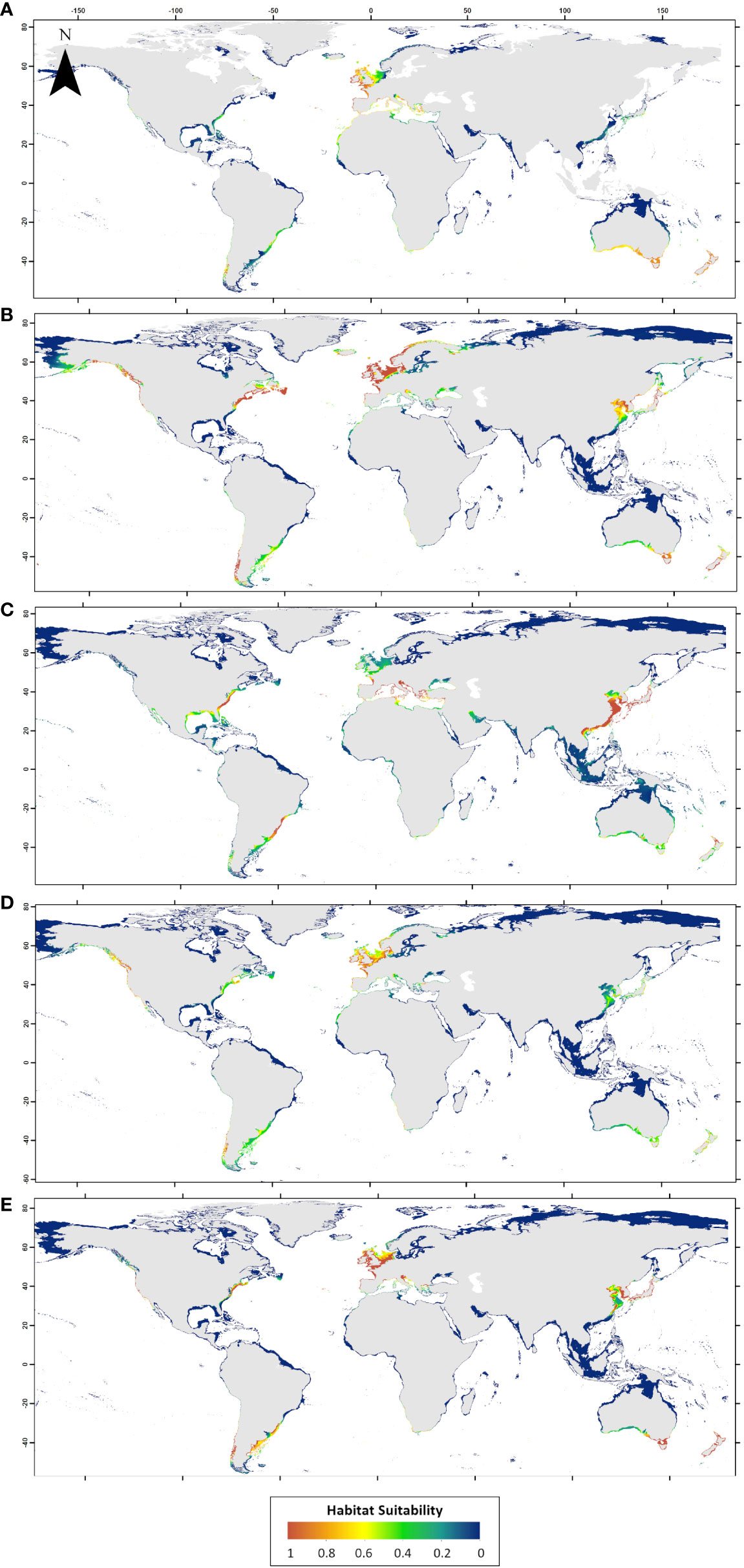
Figure 7 Final ensemble model (Weighted average) distributions for each of the five species: (A) Asparagopsis armata, (B) Bonnemaisonia hamifera, (C) Rugulopteryx okamurae, (D) Sargassum muticum and (E) Undaria pinnatifida. Darker blue colors indicate low predicted habitat suitability and warmer red colors indicate high predicted habitat suitability.
4 Discussion
The ensemble modelling approach proposed in this study has led to reliable and biologically meaningful predictions for the distributions of these five introduced and widespread seaweeds. Among the main factors considered, the enforcement of less complex models (in terms of number of predictors) does not necessarily imply better predictions. In fact, for four out of five species, models trained with large number of predictors have shown better predictions (in most cases without overfitting signs). In relation to the selection of individual algorithms and its configuration tuning, GLM and MAXENT were found to fit the most realistic responses, specifically when an intermediate complexity of its parameters was selected. An exception could be detected for small sample sizes, where GLMs showed unstable predictions.
4.1 Number of environmental predictors included in final models
There has been growing recognition that the choice of environmental predictors has important effects on model predictive power and transferability (Peterson and Nakazawa, 2007; Fourcade et al., 2018). Our findings suggest that models trained with the large dataset outperform (as they scored higher values in at least two of the three metrics analyzed) models trained with less predictors, except for R. okamurae models. Results for this species matched with those of Verbruggen et al. (2013) for Caulerpa taxifolia, in which reducing the number of predictors improved model performance. Two characteristics differentiate Rugulopteryx and Caulerpa species from the other four: 1) The history of its introduction process; 2) Small sample sizes. It is well-know that working with small samples is often problematic, as predictions are easily overfitted or inaccurate (Breiner et al., 2015). Studies on small samples and model’s complexity (e.g. Shcheglovitova and Anderson, 2013) have suggested that simpler models reduce that problem, which is consistent with our results for R. okamurae.
Overfitting can also be present when models are trained with larger environmental datasets and its detection is not always easy. Following recommendations (Hernandez et al., 2006; Breiner et al., 2015), three different metrics and visual inspection of distributions were used but evidences of overfitting were not found in those cases. Sharp transitions between high and low predicted habitat suitability values, which indicates high probabilities of over-complexity (Lake et al., 2020), were not identified from visual inspection either. Although differences between models trained with the larger and simpler predictor dataset (in terms of accuracy metrics values), whilst significant in some cases, tended to be small.
4.2 Algorithm selection and configuration tuning
Model performance metrics were good in general, but tree‐based techniques (both RF and GBM) performed better on average than the rest for each species and predictor dataset, which is consistent with some recent studies on marine species (e.g. D’Amen and Azzurro, 2020). In fact, AUC and TSS metric values for those techniques were higher than those shown for regression techniques in almost every model analysed. However, as shown in the results, some of these models were affected by overfitting, suggesting those results may be interpreted cautiously. When analysed in detail, our results revealed important model-to-model, species-to-species and metric-to-metric variability in model performance. This variability, particularly between species and metrics, highlighted the importance of tuning and selecting algorithms individually for each species and the importance of taking into consideration more than one metric. However, according to Hao et al. (2020) and Hao et al. (2019) most of ensemble modelling studies still rely on default configurations equally applied to different species. In contrast, our research proposes (in addition to model performance metrics) a second and uncommon criterion for selecting the algorithms (and its configuration) to be included in final ensembles which is the analysis of response curves. This criterion has shown to play a crucial role by discarding modelling techniques (such as RF) with unrealistic, overfitted or unstable (incongruent between replicates) response curves masked by their good model performance metrics.
Concerning algorithm configuration, MAXENT and GLM models fitted with an intermediate complexity level were the most balanced in terms of metrics and response curves quality, with the exception of R. okamurae. For this species, GLM were unstable among replicates. Bad performances of this modeling technique have already been reported when the sample size is small (Aguirre-Gutiérrez et al., 2013). MAXENT auto feature models (similar to our highest complexity configuration) have been proven to perform significantly better than simpler models (similar to our intermediate configuration) when analyzed via AUC (Syfert et al., 2013). In our analysis, MAXENT highest complexity models performed slightly better than intermediate complexity models for most species and metrics, although differences were mostly not significant (with few exceptions). However, when response curves were analyzed clear evidences of overfitting could be found for models allowing extra complexity (those allowing hinge features). On the other hand, limiting MAXENT models to linear features, and GLM to linear responses, forced the models to capture only partial responses, which resulted in worse metric values. Although, this configuration was included in the analysis as it would be a better option for modelling species where only part of the environmental range has been sampled (which is frequent in incipient introductions – e.g. R. okamurae) (Merow et al., 2014). Finally, this last theory for R. okamurae was not confirmed by our results. RF models showed few differences between configurations in terms of model performance metrics and response curves smoothness. Intermediate complexity GBMs rendered good results for R. okamurae, which is in line with some theories about these models performing better with small sample sizes (Ng and Jordan, 2001; Aguirre-Gutiérrez et al., 2013). For the other four species, characterized by larger sample sizes, intermediate and high complexity GBMs performed well according to metrics. Nevertheless, these models have been reported to be prone to overfit the training data (Elith and Graham, 2009), which was confirmed for some (but not all) species in our response curves and distributions analysis.
4.3 Introduced seaweeds distributions
Geographical distributions modelled in this study were congruent with the historical known range of the five species. For example, A. armata has been detected in four different continents, although the vast majority of records are located in Europe. It is described to be distributed from the British Isles to Senegal, including the Mediterranean Sea, the Azores and Canary Islands (Ní Chualáin et al., 2004; Andreakis et al., 2007). This widespread distribution is possible due to its photosynthetic plasticity and its tolerance to wide thermal ranges (Zanolla et al., 2014), which were correctly captured in our modelled response curves. Other conditions, such as those related to temperature variables were also correctly predicted. Kraan and Barrington (2005) suggested that gametophytes survive and grow at temperatures of 5-20°C while tetrasporophytes survive at temperatures of 5-25°C, and grow at 9-23°C. This may explain the low habitat suitability values captured by our ensemble model in its southern limits (for example in latitudes below the Canary Islands), where SSTM reached values over 22-23°C. However, there are still some important factors our model cannot capture. As an example, its long-distance dispersal ability by flotation (more noticeably in the tetrasporophyte phase) is known to play an important role in shaping its distribution. Unfortunately, this process is difficult to quantify and parameterize. More research is needed in this field, from estimating dispersal distances to understanding the environmental conditions limiting the main mechanisms for settlement. Other processes, like those related to reproduction traits, were not considered in our model either. Vegetative propagation of tetrasporophytes seems to be the main mechanism of recruitment in areas close to its distribution limits, while sexual reproduction appears to be restricted to a narrow window of temperature and light conditions in autumn (Guiry and Dawes, 1992). Understanding those patterns and finding ways to integrate them in SDMs is crucial for a better prediction of distribution limits and their expansion.
B. hamifera and A. armata share family and part of the non-native distribution range in Europe, although their origin is different. B. hamifera distribution is shifted northwards when compared to A. armata distribution, with the southernmost presences recorded in the Canary Islands and the northernmost recorded in Norway. Temperatures over 20°C have been suggested to affect reproduction, becoming lethal over 25°C (Breeman et al., 1988). Low and intermediate habitat suitability values in southern locations, such as those in the Mediterranean and Canary Islands, are explained by this temperature requirements. In northern locations, the expansion of this species is controlled by reproduction requirements which cannot be captured with the environmental variables selected. Temperatures over 10°C are needed for this process at some point of the year (Breeman et al., 1988). Including a variable accounting for the number of days exceeding 10°C, as previously done in regional studies (de la Hoz et al., 2019a), could improve model performance. However, to our knowledge, this kind of variables are not available at global scale. Other variables, such as those relative to nutrients concentrations (phosphates and nitrates), showed conflicting results for this species and A. armata. Modelled responses reflected low habitat suitability to higher rather than lower levels of those nutrients, although it has been indicated otherwise (Marcelino and Verbruggen, 2015). These do not necessary imply lower tolerance to higher concentrations but it seems more likely that they are representing the oligotrophic nature of the coastal environments at global scale.
Little information concerning R. okamurae ecophysiology can be found in the literature. In its native region, it is widely distributed in the Japanese coasts with the exception of the northern coldest areas. It was also recorded in other regions of China, Korea, the Philippines and Taiwan (Lewis and Norris, 1987). This temperate to subtropical distribution is well captured by the ensemble model, with the exception of the Philippines locations characterized by low habitat suitability values. SSTM values for this area are close to 30°C, far from the 15-20°C registered in Japanese native areas. Furthermore, this species seems to be absent in the western coasts of Korea (Hwang et al., 2009). Our model predicted these areas with intermediate habitat suitability values, reaching the lowest values in Korea Bay and Bohai Sea. Out of its native range, Verlaque et al. (2009) reported this species in the Mediterranean Thau Lagoon (France) for the first time in 2002. Mediterranean Sea conditions appear to be suitable for the development of this species as shown by the habitat suitability maps. Although, since its first report in 2002, the Strait of Gibraltar is the only location where this species is established (besides Thau Lagoon) (García-Gómez et al., 2020). Even though results were in close agreement with the known range, distributions must be interpreted cautiously as models were constructed using a small number of presences.
Experimental studies for S. muticum have shown that adult individuals can survive in temperatures between -1°C and 30°C, which are similar to the seasonal ranges in native areas (Norton, 1977; Hales and Fletcher, 1990). Our modelled responses for SSTM were more restrictive, with the lowest habitat suitability values over 25°C and below 5°C. MAXENT was the most restrictive model, establishing the upper tolerance limit in 20°C. Low temperatures (below 10°C) have been demonstrated to reduce fertilization and post-fertilization development and limit the germlings growth (Steen and Rueness, 2004), which may be an explanation for the low habitat suitability values at those temperatures. Unlike the other species (except for B. hamifera), models for S. muticum suggested that its distribution is not limited to areas with salinity values over 30‰. Experiments have shown that this species can survive salinities below 10‰ (Norton, 1977; Hales and Fletcher, 1990), reason why this species can be found in brackish areas such as the Baltic Sea (Leppäkoski and Olenin, 2000). In addition, our modelled non-native distribution in Europe is congruent with that reported in regional studies (de la Hoz et al., 2019a) or hybrid modelling approaches (Chefaoui et al., 2019). Southern locations in the Mediterranean Sea received low habitat suitability values in general, except for two particular locations (Thau Lagoon in France and Venice Lagoon in Italy) where the species have been reported to be established. In fact, Mediterranean environmental conditions seem to be unfavorable for the settlement of this species, as only drifting material has been found outside these two locations (Engelen et al., 2015).
U. pinnatifida tolerance to large annual temperature fluctuations explains why this species is widely distributed in Europe, Australia, New Zealand and North and South America (James et al., 2015). According to our modelled distribution, the southern coasts of Norway seems to be its northern limit in Europe as regions over these latitudes present habitat suitability values close to zero. In contrast, other studies have suggested the Barents Sea to be its northern limit of expansion (Minchin and Nunn, 2014). In southern Europe, Portuguese and Spanish locations in the Atlantic Ocean showed very favorable conditions for the establishment of this species. Even though, it is known that this species is restricted to a few locations in northern Portugal and the western part of the Bay of Biscay (Blanco et al., 2021). Variables such as the influence of adjacent river basins or human activities on nutrient concentration and chlorophyll-A seemed to control their distribution at this regional scale (Báez et al., 2010). Additionally, there were still some other patterns this modelling approach was not able to capture. For example, sporophyte recruitment needs temperatures between 5-20°C, reaching the highest rates at 13-17°C. Considering those ranges, it seems unlikely to find this species in the northeastern Iberian coasts, where sea surface temperatures reach values over 20°C in summer. Better predictions, not only at regional scales, require models that include this kind of physiological information. Identifying the key processes, characterizing it in laboratory or field experiments and then parameterizing it into response curves could be a first step to be considered in future research.
In conclusion, ensemble modelling non-native seaweeds distributions has shown to be still a challenging process as several factors influence the quality of the predictions. This research highlights the importance of exploring different environmental predictors combinations, algorithms and setting configurations in ensembles for each seaweed individually to achieve ecologically meaningful results. Additionally, our results suggest that integrating ecological realism as a qualitative criterion for selecting the optimal models to be included in the ensemble, helps improve the final predictions. Although requiring further development (particularly from a physiological point of view), our ensemble modelling approach properly captured the known locations for these five seaweeds and the possible areas of expansion. Understanding these distributional patterns and finding ways to improve the modelling techniques have several implications not only from a biogeographical point of view, but also for management issues. Accurate predictions will help managers to take more effective actions to reduce or prevent the negative effects these alien species generate in local biodiversity and economy.
Data availability statement
Presence points datasets for each species are available in Supplementary Material 3. Information concerning environmental predictors used to trained the models and details about how to acquire it are provided in the main text and Supplementary Material 1 (Table S1.2). Final ensemble maps are also provided in GeoTiff format for reuse. An example of the R workflow applied to one species is also provided. Any other intermediate dataset will be provided by the corresponding author upon reasonable request.
Author contributions
SS-V, CH, JJ and AP authors conceived the study. SS-V and CH acquired the data. SS-V performed analyses and led the writing. All authors contributed by editing the manuscript and gave final approval for publication.
Funding
This work was funded by the National Plan for Research in Science and Technological Innovation from the Spanish Government 2017-2020 [grant number C3N-pro project PID2019-105503RB-I00] and co-funded by the European Regional Development’s funds. SS-V acknowledges financial support under a predoctoral grant from the Spanish Ministry of Education and Vocational Training [grant number: FPU18/03573]. CH acknowledges the financial support from the Government of Cantabria through the Fénix Programme and under a postdoctoral grant from the University of Cantabria [grant number: POS-UC-2020-07]. This work is part of the PhD project of SS-V.
Conflict of interest
The authors declare that the research was conducted in the absence of any commercial or financial relationships that could be construed as a potential conflict of interest.
Publisher’s note
All claims expressed in this article are solely those of the authors and do not necessarily represent those of their affiliated organizations, or those of the publisher, the editors and the reviewers. Any product that may be evaluated in this article, or claim that may be made by its manufacturer, is not guaranteed or endorsed by the publisher.
Supplementary material
The Supplementary Material for this article can be found online at: https://www.frontiersin.org/articles/10.3389/fmars.2022.1009808/full#supplementary-material
References
Aguirre-Gutiérrez J., Carvalheiro L. G., Polce C., van Loon E. E., Raes N., Reemer M., et al. (2013). Fit-for-Purpose: Species distribution model performance depends on evaluation criteria – Dutch hoverflies as a case study. PLoS One 8, e63708. doi: 10.1371/journal.pone.0063708
Aiello-Lammens M. E., Boria R. A., Radosavljevic A., Vilela B., Anderson R. P. (2015). spThin: An r package for spatial thinning of species occurrence records for use in ecological niche models. Ecography (Cop.) 38, 541–545. doi: 10.1111/ecog.01132
Allouche O., Tsoar A., Kadmon R. (2006). Assessing the accuracy of species distribution models: Prevalence, kappa and the true skill statistic (TSS). J. Appl. Ecol. 43, 1223–1232. doi: 10.1111/j.1365-2664.2006.01214.x
Anderson R. P., Gonzalez I. (2011). Species-specific tuning increases robustness to sampling bias in models of species distributions: An implementation with maxent. Ecol. Modell. 222, 2796–2811. doi: 10.1016/j.ecolmodel.2011.04.011
Andreakis N., Procaccini G., Maggs C. A., Kooistra W. H. C. F. (2007). Phylogeography of the invasive seaweed Asparagopsis (Bonnemaisoniales, rhodophyta) reveals cryptic diversity. Mol. Ecol. 16, 2285–2299. doi: 10.1111/j.1365-294X.2007.03306.x
Araújo M. B., New M. (2007). Ensemble forecasting of species distributions. Trends Ecol. Evol. 22, 42–47. doi: 10.1016/j.tree.2006.09.010
Araújo M. B., Pearson R. G. (2005). Equilibrium of species’ distributions with climate. Ecography (Cop.) 28, 693–695. doi: 10.1111/j.2005.0906-7590.04253.x
Assis J., Tyberghein L., Bosch S., Verbruggen H., Serrão E. A., De Clerck O. (2018). Bio-ORACLE v2.0: Extending marine data layers for bioclimatic modelling. Glob. Ecol. Biogeogr. 27, 277–284. doi: 10.1111/geb.12693
Báez J. C., Olivero J., Peteiro C., Ferri-Yáñez F., Garcia-Soto C., Real R. (2010). Macro-environmental modelling of the current distribution of Undaria pinnatifida (Laminariales, ochrophyta) in northern Iberia. Biol. Invasions 12, 2131–2139. doi: 10.1007/s10530-009-9614-1
Barbet-Massin M., Jiguet F., Albert C. H., Thuiller W. (2012). Selecting pseudo-absences for species distribution models: How, where and how many? Methods Ecol. Evol. 3, 327–338. doi: 10.1111/j.2041-210X.2011.00172.x
Bathke A. C., Harrar S. W. (2016). “Rank-based inference for multivariate data in factorial designs,” in Robust rank-based and nonparametric methods. springer proceedings in mathematics & statistics, vol. 168 . Eds. Liu R., McKean. J. (Cham: Springer), 121–139. doi: 10.1007/978-3-319-39065-9_7
Blanco A., Larrinaga A. R., Neto J. M., Troncoso J., Méndez G., Domínguez-Lapido P., et al. (2021). Spotting intruders: Species distribution models for managing invasive intertidal macroalgae. J. Environ. Manage 281, 111861. doi: 10.1016/j.jenvman.2020.111861
Boyce M. S., Vernier P. R., Nielsen S. E., Schmiegelow F. K. (2002). Evaluating resource selection functions. Ecol. Modell. 157, 281–300. doi: 10.1016/S0304-3800(02)00200-4
Breeman A. M., Meulenhoff E. J. S., Guiry M. D. (1988). Life history regulation and phenology of the red alga Bonnemaisonia hamifera. Helgoländer Meeresuntersuchungen 42, 535–551. doi: 10.1007/BF02365625
Breiner F. T., Guisan A., Bergamini A., Nobis M. P. (2015). Overcoming limitations of modelling rare species by using ensembles of small models. Methods Ecol. Evol. 6, 1210–1218. doi: 10.1111/2041-210X.12403
Chefaoui R. M., Serebryakova A., Engelen A. H., Viard F., Serrão E. A. (2019). Integrating reproductive phenology in ecological niche models changed the predicted future ranges of a marine invader. Divers. Distrib. 25, 688–700. doi: 10.1111/ddi.12910
D’Amen M., Azzurro E. (2020). Integrating univariate niche dynamics in species distribution models: A step forward for marine research on biological invasions. J. Biogeogr. 47, 686–697. doi: 10.1111/jbi.13761
de la Hoz C. F., Ramos E., Puente A., Juanes J. A. (2019a). Climate change induced range shifts in seaweeds distributions in Europe. Mar. Environ. Res. 148, 1–11. doi: 10.1016/j.marenvres.2019.04.012
de la Hoz C. F., Ramos E., Puente A., Juanes J. A. (2019b). Temporal transferability of marine distribution models: The role of algorithm selection. Ecol. Indic. 106, 105499. doi: 10.1016/j.ecolind.2019.105499
Di Cola V., Broennimann O., Petitpierre B., Breiner F. T., D’Amen M., Randin C., et al. (2017). Ecospat: An r package to support spatial analyses and modeling of species niches and distributions. Ecography (Cop.) 40, 774–787. doi: 10.1111/ecog.02671
Elith J., Graham C. H. (2009). Do they? How do they? Why do they differ? on finding reasons for differing performances of species distribution models. Ecography (Cop.) 32, 66–77. doi: 10.1111/j.1600-0587.2008.05505.x
Elith J., Kearney M., Phillips S. J. (2010). The art of modelling range-shifting species. Methods Ecol. Evol. 1, 330–342. doi: 10.1111/j.2041-210X.2010.00036.x
Elith J., Leathwick J. R., Hastie T. (2008). A working guide to boosted regression trees. J. Anim. Ecol. 77, 802–813. doi: 10.1111/j.1365-2656.2008.01390.x
Engelen A. H., Serebryakova A., Ang P., Britton-Simmons K. H., Mineur F., Pedersen M. F., et al. (2015). “Circumglobal invasion by the brown seaweed sargassum muticum,” in Oceanography and marine biology: An annual review oceanography and marine biology. Eds. Hughes R. N., Hughes D. J., Smith I. P., Dale A. C. (Boca Raton, FL: Taylor & Francis), 81–126.
Fourcade Y., Besnard A. G., Secondi J. (2018). Paintings predict the distribution of species, or the challenge of selecting environmental predictors and evaluation statistics. Glob. Ecol. Biogeogr. 27, 245–256. doi: 10.1111/geb.12684
Fourcade Y., Engler J. O., Rödder D., Secondi J. (2014). Mapping species distributions with MAXENT using a geographically biased sample of presence data: A performance assessment of methods for correcting sampling bias. PLoS One 9, e97122. doi: 10.1371/journal.pone.0097122
Franklin J. (2010). Mapping species distributions (Cambridge: Cambridge University Press). doi: 10.1017/CBO9780511810602
Friedman J. H. (2001). Greedy function approximation: A gradient boosting machine. Ann. Stat. 29, 1189–1232. doi: 10.1214/aos/1013203451
García-Gómez J. C., Sempere-Valverde J., González A. R., Martínez-Chacón M., Olaya-Ponzone L., Sánchez-Moyano E., et al. (2020). From exotic to invasive in record time: The extreme impact of Rugulopteryx okamurae (Dictyotales, ochrophyta) in the strait of Gibraltar. Sci. Total Environ. 704, 135408. doi: 10.1016/j.scitotenv.2019.135408
GBIF (2021) What is GBIF? Available at: https://www.gbif.org/what-is-gbif.
GEBCO Bathymetric Compilation Group (2020). The GEBCO2020 grid - a continuous terrain model of the global oceans and land (UK: British Oceanographic Data Centre, National Oceanography Centre, NERC). doi: 10.5285/a29c5465-b138-234d-e053-6c86abc040b9
Guiry M. D., Dawes C. J. (1992). Daylength, temperature and nutrient control of tetrasporogenesis in Asparagopsis armata (Rhodophyta). J. Exp. Mar. Bio. Ecol. 158, 197–217. doi: 10.1016/0022-0981(92)90227-2
Guisan A., Thuiller W., Zimmermann N. E. (2017). Habitat suitability and distribution models (Cambridge: Cambridge University Press). doi: 10.1017/9781139028271
Hales J. M., Fletcher R. L. (1990). Studies on the recently introduced brown alga Sargassum muticum (Yendo) fensholt. v.: Receptacle initiation and growth, and gamete release in laboratory culture. Bot. Mar. 33, 167–176. doi: 10.1515/botm.1990.33.3.241
Hallgren W., Santana F., Low-Choy S., Rehn J. H. K., Mackey B. (2017). “Sensitivity analysis to configuration option settings in a selection of species distribution modelling algorithms,” in MODSIM2017- 22nd international congress on modelling and simulation (Australia: Modelling and Simulation Society of Australia and New Zealand), vol. 894–900. doi: 10.36334/MODSIM.2017.A1.Hallgren
Hallgren W., Santana F., Low-Choy S., Zhao Y., Mackey B. (2019). Species distribution models can be highly sensitive to algorithm configuration. Ecol. Modell. 408, 108719. doi: 10.1016/j.ecolmodel.2019.108719
Hanley J. A., McNeil B. J. (1982). The meaning and use of the area under a receiver operating characteristic (ROC) curve. Radiology 143, 29–36. doi: 10.1148/radiology.143.1.7063747
Hao T., Elith J., Guillera-Arroita G., Lahoz-Monfort J. J. (2019). A review of evidence about use and performance of species distribution modelling ensembles like BIOMOD. Divers. Distrib. 25, 839–852. doi: 10.1111/ddi.12892
Hao T., Elith J., Lahoz-Monfort J. J., Guillera-Arroita G. (2020). Testing whether ensemble modelling is advantageous for maximising predictive performance of species distribution models. Ecography (Cop.) 43, 549–558. doi: 10.1111/ecog.04890
Hernandez P. A., Graham C. H., Master L. L., Albert D. L. (2006). The effect of sample size and species characteristics on performance of different species distribution modeling methods. Ecography (Cop.) 29, 773–785. doi: 10.1111/j.0906-7590.2006.04700.x
Hirzel A. H., Le Lay G., Helfer V., Randin C., Guisan A. (2006). Evaluating the ability of habitat suitability models to predict species presences. Ecol. Modell. 199, 142–152. doi: 10.1016/j.ecolmodel.2006.05.017
Hwang I.-K., Lee W. J., Kim H.-S., De Clerck O. (2009). Taxonomic reappraisal of dilophus okamurae (Dietyotales, phaeophyta) from the western pacific ocean. Phycologia 48, 1–12. doi: 10.2216/07-68.1
James K., Kibele J., Shears N. T. (2015). Using satellite-derived sea surface temperature to predict the potential global range and phenology of the invasive kelp Undaria pinnatifida. Biol. Invasions 17, 3393–3408. doi: 10.1007/s10530-015-0965-5
Kiefel M., Bathke A. C. (2020). “Rank-based analysis of multivariate data in factorial designs and its implementation in r,” in Nonparametric statistics. ISNPS 2018. springer proceedings in mathematics & statistics, vol. 339 . Eds. La Rocca M., Liseo B., Salmaso L. (Cham: Springer). doi: 10.1007/978-3-030-57306-5_26
Kraan S., Barrington K. A. (2005). Commercial farming of Asparagopsis armata (Bonnemaisoniceae, rhodophyta) in Ireland, maintenance of an introduced species? J. Appl. Phycol. 17, 103–110. doi: 10.1007/s10811-005-2799-5
Lake T. A., Briscoe Runquist R. D., Moeller D. A. (2020). Predicting range expansion of invasive species: Pitfalls and best practices for obtaining biologically realistic projections. Divers. Distrib. 26, 1767–1779. doi: 10.1111/ddi.13161
Leppäkoski E., Olenin S. (2000). Non-native species and rates of spread: Lessons from the brackish Baltic Sea. Biol. Invasions 2, 151–163. doi: 10.1023/A:1010052809567
Lewis J. L., Norris J. N. (1987). A history and annotated account of the benthic marine algae of Taiwan. Smithson. Contrib. Mar. Sci. 29, iv–38. doi: 10.5479/si.01960768.29.iv
Lüning K., Yarish C., Kirkman H. (1990). Seaweeds: their environment, biogeography, and ecophysiology (New York, USA: Wiley). doi: 10.1002/aqc.3270010208
Marcelino V. R., Verbruggen H. (2015). Ecological niche models of invasive seaweeds. J. Phycol. 51, 606–620. doi: 10.1111/jpy.12322
Marmion M., Parviainen M., Luoto M., Heikkinen R. K., Thuiller W. (2009). Evaluation of consensus methods in predictive species distribution modelling. Divers. Distrib. 15, 59–69. doi: 10.1111/j.1472-4642.2008.00491.x
Martínez B., Arenas F., Trilla A., Viejo R. M., Carreño F. (2015). Combining physiological threshold knowledge to species distribution models is key to improving forecasts of the future niche for macroalgae. Glob. Change Biol. 21, 1422–1433. doi: 10.1111/gcb.12655
Martínez B., Viejo R. M., Carreño F., Aranda S. C. (2012). Habitat distribution models for intertidal seaweeds: Responses to climatic and non-climatic drivers. J. Biogeogr. 39, 1877–1890. doi: 10.1111/j.1365-2699.2012.02741.x
McCullagh P., Nelder J. A. (1983). Generalized linear models (New York, USA: Chapman and Hall Routledge). doi: 10.1201/9780203753736
Melo-Merino S. M., Reyes-Bonilla H., Lira-Noriega A. (2020). Ecological niche models and species distribution models in marine environments: A literature review and spatial analysis of evidence. Ecol. Modell. 415, 108837. doi: 10.1016/j.ecolmodel.2019.108837
Merow C., Smith M. J., Edwards T. C., Guisan A., McMahon S. M., Normand S., et al. (2014). What do we gain from simplicity versus complexity in species distribution models? Ecography (Cop.) 37, 1267–1281. doi: 10.1111/ecog.00845
Merow C., Smith M. J., Silander J. A. (2013). A practical guide to MaxEnt for modeling species’ distributions: what it does, and why inputs and settings matter. Ecography (Cop.) 36, 1058–1069. doi: 10.1111/j.1600-0587.2013.07872.x
MHE (2021) Macroalgal herbarium consortium portal. Available at: https://macroalgae.org/portal/.
Minchin D., Nunn J. (2014). The invasive brown alga Undaria pinnatifida (Harvey) suringar 1873 (Laminariales: Alariaceae), spreads northwards in Europe. BioInvasions Rec. 3, 57–63. doi: 10.3391/bir.2014.3.2.01
Morales N. S., Fernández I. C., Baca-González V. (2017). MaxEnt’s parameter configuration and small samples: Are we paying attention to recommendations? A systematic review. PeerJ 2017, 1–16. doi: 10.7717/peerj.3093
Munzel U., Brunner E. (2000). Nonparametric methods in multivariate factorial designs. J. Stat. Plan. Inference 88, 117–132. doi: 10.1016/S0378-3758(99)00212-8
Ng A. Y., Jordan M. I. (2001). “On discriminative vs. generative classifiers: A comparison of logistic regression and naive bayes,” in Proceedings of the 14th international conference on neural information processing systems: Natural and synthetic NIPS’01 (Cambridge, MA, USA: MIT Press), 841–848.
Ní Chualáin F., Maggs C. A., Saunders G. W., Guiry M. D. (2004). The invasive genus Asparagopsis (Bonnemaisoniaceae, rhodophyta): Molecular systematics, morphology, and ecophysiology of falkenbergia isolates. J. Phycol. 40, 1112–1126. doi: 10.1111/j.1529-8817.2004.03135.x
Norton T. A. (1977). Ecological experiments with sargassum muticum. j. mar. biol. assoc Vol. 57 (Cambridge University Press: United Kingdom), 33–43. doi: 10.1017/S0025315400021214
OBIS (2021) Ocean biodiversity information system. Available at: https://obis.org/.
Peterson A. T., Nakazawa Y. (2007). Environmental data sets matter in ecological niche modelling: an example with solenopsis invicta and solenopsis richteri. Glob. Ecol. Biogeogr. 17, 135–144. doi: 10.1111/j.1466-8238.2007.00347.x
Peterson A. T., Soberón J., Pearson R. G., Anderson R. P., Martínez-Meyer E., Nakamura M., et al. (2011). Ecological niches and geographic distributions (MPB-49) (New Jersey, USA: Princeton University Press). doi: 10.2307/j.ctt7stnh
Petitpierre B., Broennimann O., Kueffer C., Daehler C., Guisan A. (2017). Selecting predictors to maximize the transferability of species distribution models: Lessons from cross-continental plant invasions. Glob. Ecol. Biogeogr. 26, 275–287. doi: 10.1111/geb.12530
Phillips S. J., Anderson R. P., Dudík M., Schapire R. E., Blair M. E. (2017). Opening the black box: An open-source release of maxent. Ecography (Cop.) 40, 887–893. doi: 10.1111/ecog.03049
Phillips S. J., Anderson R. P., Schapire R. E. (2006). Maximum entropy modeling of species geographic distributions. Ecol. Modell 190, 231–259. doi: 10.1016/j.ecolmodel.2005.03.026
Radosavljevic A., Anderson R. P. (2014). Making better maxent models of species distributions: Complexity, overfitting and evaluation. J. Biogeogr. 41, 629–643. doi: 10.1111/jbi.12227
R Core Team (2020) R: A language and environment for statistical computing. Available at: https://www.r-project.org/.
Robinson L. M., Elith J., Hobday A. J., Pearson R. G., Kendall B. E., Possingham H. P., et al. (2011). Pushing the limits in marine species distribution modelling: Lessons from the land present challenges and opportunities. Glob. Ecol. Biogeogr. 20, 789–802. doi: 10.1111/j.1466-8238.2010.00636.x
Schaffelke B., Smith J. E., Hewitt C. L. (2006). Introduced macroalgae – a growing concern. J. Appl. Phycol. 18, 529–541. doi: 10.1007/s10811-006-9074-2
Sequeira A. M. M., Bouchet P. J., Yates K. L., Mengersen K., Caley M. J. (2018). Transferring biodiversity models for conservation: Opportunities and challenges. Methods Ecol. Evol. 9, 1250–1264. doi: 10.1111/2041-210X.12998
Shcheglovitova M., Anderson R. P. (2013). Estimating optimal complexity for ecological niche models: A jackknife approach for species with small sample sizes. Ecol. Modell. 269, 9–17. doi: 10.1016/j.ecolmodel.2013.08.011
Steen H., Rueness J. (2004). Comparison of survival and growth in germlings of six fucoid species (Fucales, phaeophyceae) at two different temperature and nutrient levels. Sarsia 89, 175–183. doi: 10.1080/00364820410005818
Syfert M. M., Smith M. J., Coomes D. A. (2013). The effects of sampling bias and model complexity on the predictive performance of MAXENT species distribution models. PLoS One 8, e55158. doi: 10.1371/journal.pone.0055158
Thuiller W. (2004). Patterns and uncertainties of species’ range shifts under climate change. Glob. Change Biol. 10, 2020–2027. doi: 10.1111/j.1365-2486.2004.00859.x
Thuiller W., Guéguen M., Renaud J., Karger D. N., Zimmermann N. E. (2019). Uncertainty in ensembles of global biodiversity scenarios. Nat. Commun. 10, 1446. doi: 10.1038/s41467-019-09519-w
Thuiller W., Lafourcade B., Engler R., Araújo M. B. (2009). BIOMOD - A platform for ensemble forecasting of species distributions. Ecography (Cop.) 32, 369–373. doi: 10.1111/j.1600-0587.2008.05742.x
Valavi R., Guillera-Arroita G., Lahoz-Monfort J. J., Elith J. (2022). Predictive performance of presence-only species distribution models: A benchmark study with reproducible code. Ecol. Monogr. 92, e01486. doi: 10.1002/ecm.1486
Verbruggen H., Tyberghein L., Belton G. S., Mineur F., Jueterbock A., Hoarau G., et al. (2013). Improving transferability of introduced species’ distribution models: New tools to forecast the spread of a highly invasive seaweed. PLoS One 8, e68337. doi: 10.1371/journal.pone.0068337
Verlaque M., Steen F., De Clerck O. (2009). Rugulopteryx (Dictyotales, phaeophyceae), a genus recently introduced to the Mediterranean. Phycologia 48, 536–542. doi: 10.2216/08-103.1
Zanolla M., Carmona R., de la Rosa J., Salvador N., Sherwood A., Andreakis N., et al. (2014). Morphological differentiation of cryptic lineages within the invasive genus Asparagopsis (Bonnemaisoniales, rhodophyta). Phycologia 53, 233–242. doi: 10.2216/13-247.1
Zhang L., Liu S., Sun P., Wang T., Wang G., Zhang X., et al. (2015). Consensus forecasting of species distributions: The effects of niche model performance and niche properties. PLoS One 10, e0120056. doi: 10.1371/journal.pone.0120056
Keywords: ensemble, invasive, macroalgae, non-native, seaweeds, species distribution models
Citation: Sainz-Villegas S, de la Hoz CF, Juanes JA and Puente A (2022) Predicting non-native seaweeds global distributions: The importance of tuning individual algorithms in ensembles to obtain biologically meaningful results. Front. Mar. Sci. 9:1009808. doi: 10.3389/fmars.2022.1009808
Received: 02 August 2022; Accepted: 02 November 2022;
Published: 18 November 2022.
Edited by:
Tommaso Russo, University of Rome Tor Vergata, ItalyReviewed by:
Thomas Groen, University of Twente, NetherlandsDimitris Poursanidis, Terrasolutions Marine Environment Research, Greece
Copyright © 2022 Sainz-Villegas, de la Hoz, Juanes and Puente. This is an open-access article distributed under the terms of the Creative Commons Attribution License (CC BY). The use, distribution or reproduction in other forums is permitted, provided the original author(s) and the copyright owner(s) are credited and that the original publication in this journal is cited, in accordance with accepted academic practice. No use, distribution or reproduction is permitted which does not comply with these terms.
*Correspondence: Samuel Sainz-Villegas, c2FtdWVsLnNhaW56QHVuaWNhbi5lcw==