CPUE retrieval from spaceborne lidar data: A case study in the Atlantic bigeye tuna fishing area and Antarctica fishing area

The measurement of Catch Per Unit Effort (CPUE) supports the assessment of status and trends by managers. This proportion of total catch to the harvesting effort estimates the abundance of fishery resources. Marine environmental data obtained by satellite remote sensing are essential in fishing efficiency estimation or CPUE standardization. Currently, remote sensing chlorophyll data used for fisheries resource assessment are mainly from passive ocean color remote sensing. However, high-resolution data are not available at night or in high-latitude areas such as polar regions due to insufficient solar light, clouds, and other factors. In this paper, a CPUE inversion method based on spaceborne lidar data is proposed, which is still feasible for polar regions and at nighttime. First, Atlantic bigeye tuna CPUE was modeled using Cloud aerosol lidar and infrared pathfinder satellite observations (CALIPSO) lidar-retrieved chlorophyll data in combination with sea surface temperature data. The Generalized Linear Model (GLM), Artificial Neural Network (ANN) and Support Vector Machine Methods (SVM) were used for modeling, and the three methods were compared and validated. The results showed that the correlation between predicted CPUE and nominal CPUE was higher for the ANN method, with an R² of 0.34, while the R² was 0.08 and 0.22 for GLM and SVM, respectively. Then, chlorophyll data in the polar regions were derived using CALIPSO diurnal data, and an ANN was used for Antarctic krill. The inversion result performed well, and it showed that the R² of the predicted CPUE to nominal CPUE was 0.92. Preliminary results suggest that (1) nighttime measurements can increase the understanding of the diurnal variability of the upper ocean; (2) CALIPSO measurements in polar regions fill the gap of passive measurements; and (3) comparison with field data shows that ANN-based lidar products perform well, and a neural network approach based on CALIPSO lidar data can be used to simulate CPUE inversions in polar regions.

1 Introduction

Catch Per Unit Effort (CPUE) is essential data in the assessment and management of fishery resources. CPUE is proportional to the abundance of fishery resources and serves as an important relative index of fishery resource abundance (Chen et al., 2008). During the assessment, a linear relationship between CPUE and abundance was assumed, but commercial production data were strongly influenced by temporal factors, spatial factors, environmental factors, and fishing capacity (Harley et al., 2001; Erisman et al., 2011). To use more reliable and representative CPUE data during assessment, it is necessary to standardize the nominal CPUE data using a statistical model (Maunder and Langley, 2004; Maunder and Punt, 2004). Thus the quality of standardized CPUE data and the predictability of consistent and stable models can be improved to provide better support for the assessment and management of fisheries resources (Ward et al., 2013). Marine environmental data obtained by satellite remote sensing are often essential in fishing efficiency estimation or CPUE standardization (Guan et al., 2017).

Research by marine scientists on the standardization of fisheries data began at the end of the last century (Maunder and Langley, 2004). Bigelow et al. (1999) standardized the CPUE using data such as sea surface temperature (SST) and chlorophyll_a concentration (Chl_a). Daisuke Ochi et al. (2014) standardized the Japanese bigeye tuna CPUE from 1960 to 2013 using Generalized Linear Model (GLM) and found that the trend of CPUE varied by region. The knowledge and research on fisheries data standardization in China is relatively late, and most of the literature reports are found in the last decade (Guan et al., 2014). (Chen et al., 2011) developed a habitat model based on quantile regression to evaluate the habitat quality of yellowtail forage fisheries in the Yellow Sea in winter using SST and Chl_a concentrations. The results found that habitat indices were positively correlated with CPUE when only SST and Chl_a were considered. Shi et al. (2020) standardized the CPUE of the Northwest Pacific fallfish fishery in mainland China by combining the statistical data of fallfish fishery production in the Northwest Pacific Ocean from 2003 to 2017 with the marine environmental data obtained from satellite remote sensing. Among these CPUE normalization models, the GLM and the Generalized Additive Model (GAM) are two traditional approaches (Venables and Dichmont, 2004), with GLM being the most commonly used. These two models are simple and easy to operate and can be computed by user-friendly software (Rodríguez-Marín et al., 2003). However, both methods have significant disadvantages, such as false assumptions and cross-term processing (Yu et al., 2013). Later, several nonlinear techniques were applied to standardize CPUE data, such as artificial neural networks (ANN) and Support Vector Machine (SVM) methods. ANN has better nonlinear mapping capabilities and can achieve higher prediction results compared to traditional GLM and GAM approaches (Yang et al., 2015). SVM has several theoretical advantages, such as it has no local minima in the learning phase (Huang et al., 2004) and has increased generalization performance over a limited number of training samples (Mountrakis et al., 2011).

Globally, the application of remote sensing in fisheries is increasing (Perez et al., 2013), and the use of SST and Chl_a parameters can provide insight into the marine environment and help explore fishery resources (Kamei et al., 2014). Currently, remote sensing data for fisheries resource assessment are mainly derived from passive remote sensing, such as the Moderate Resolution Imaging Spectra radiometer (MODIS). However, high-resolution Chl_a data cannot be acquired at night and in high-latitude areas such as polar regions due to factors such as spatial resolution (Guan et al., 2017), insufficient solar light (Lu et al., 2020), and clouds (Babin et al., 2015). In addition, passive remote sensing can only measure the surface or near surface of the ocean and data on the internal spatial structure of the ocean cannot be retrieved (Liu et al., 2018). In contrast, lidar as an active remote sensing technique, has the advantages of rapidity and high resolution (Chen et al., 2019) and can characterize the vertical structure of water bodies in favorable weather conditions and at high spatial resolution. Lidar has a wide range of applications, such as (1) fish detection (Churnside, 1999; Churnside et al., 2011), (2) plankton layer (Churnside, 2007; Churnside and Donaghay, 2009), (3) bathymetry (Irish et al., 2000), and (4) air bubbles (Churnside, 2013) and measurements of (1) ocean surface roughness and (2) wave detection through the interpretation of phytoplankton characteristics (Betz, 2015). Cloud aerosol lidar and infrared pathfinder satellite observations (CALIPSO) launched by NASA provides imagery that supports the characterization of the vertical structure of plankton near the ocean surface (Lu et al., 2021). The orthogonally polarized cloud aerosol lidar (CALIOP) carried on CALIPSO is the first dual-polarized lidar to provide a global vertical profile of diurnal elastic backscatter (Lu et al., 2014). However, few studies have used lidar technology to standardize CPUE.

In this paper, bigeye tuna and Antarctic krill were selected as the training data for CPUE standardization. Bigeye tuna are highly migratory species inhabiting tropical or temperate waters, with high densities near the equator, while Antarctic krill are distributed in the Antarctic region. In both regions, passive remote sensing limitations are attributed to missing data, which demonstrates the importance of ultisensory approaches. The inversion of Chl_a using Lidar data can compensate for the missing data, thus demonstrating the utility of active remote sensing. A three-step process was applied to populate data gaps. First, the CALIPSO data were preprocessed and then the CALIPSO data were used to retrieve Chl_a. Secondly, retrieved Chl_a and SST data were matched with fishery data, and the latitude and longitude of CPUE were used as criteria for gridding these environmental variable data. After that, the Atlantic bigeye tuna CPUE and its influencing factors were modeled using GLM, ANN and SVM models. The effectiveness of the three modeling approaches was validated and compared. Finally, the ANN model was applied to model and predict the CPUE of polar Antarctic krill. The main highlights of this paper are as follows: (1) Nighttime measurements increase knowledge of upper ocean diurnal variability; (2) CALIPSO measurements in the polar regions fill passive measurement gaps; and (3) Comparison with in situ data indicates that ANN-based lidar products provide valid CPUE estimates.

2 Materials and methods

2.1 Study area

The catch data of bigeye tuna (Thunnus obesus) from 2008 to 2015 were selected as the model training data. Bigeye tuna are a warm-water fish, and the production fisheries are mainly located in equatorial tropical waters and deep-sea basins, such as the Gambia Basin, Sierra Leone Basin and Brazil Deep Sea Basin. The Central Atlantic Ocean mainly consists of deep-sea basins and the Atlantic Ridge with few islands. Therefore, the central Atlantic tuna fishing area was selected as the study area. Figure 1 shows the study area and monthly CPUE statistics for this paper, the specific study area is 30°S-20°N, 60°W-20°E (Figure 1A). Fishing is mainly concentrated on the west coast of Africa, with the highest CPUE values occurring near the equator (20°W-4°E, 6°S-6°N) and decreasing from there. CPUE is divided into four ranges: less than 1.81; 1.81 to 6.53; 6.53 to 13.8, and more than 13.8 tons/hour (t/h). The highest CPUE is found in the Guinea Basin and its southwestern waters, with a range greater than 13.8 t/h.

FIGURE 1

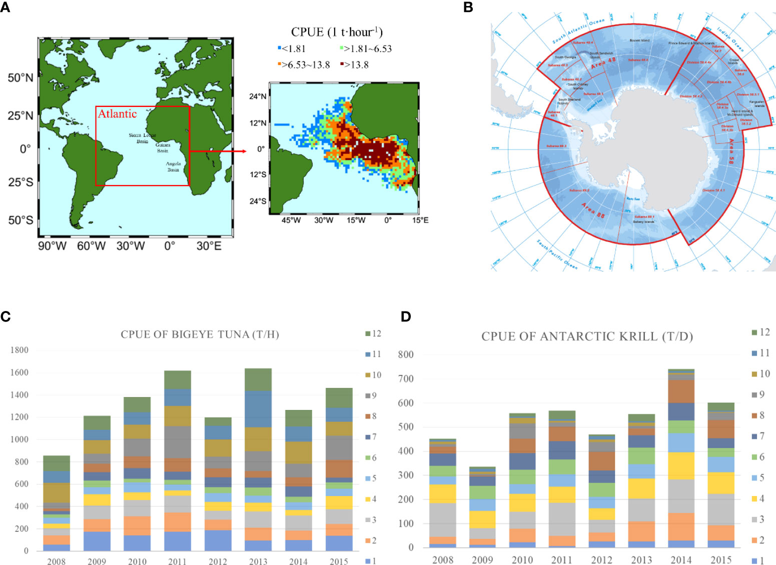
Figure 1 shows the study area and CPUE statistics, (A, B) are maps of the main fishing areas in the Atlantic Ocean and Antarctica, respectively; (C, D) are monthly CPUE statistics for bigeye tuna and Antarctic krill, respectively, from 2008 to 2015. Where X-axis indicates the year, Y-axis indicates the value of CPUE, and 1 to 12 are the months, indicating the CPUE values for each month of the year; the unit of CPUE for tuna is T/H, indicating the number of tons (T) caught per hour (H), and the unit of CPUE for Antarctic krill is T/D, indicating the number of tons (T) caught per day (D).

The catch data of Antarctic krill (Euphausia superba) from 2008 to 2015 were selected as the polar model training data. Antarctic krill are a species of krill that live in the Antarctic waters of the Southern Ice Ocean, and fishing operations are mainly in the South Atlantic region. Figure 1B shows a map of the main fishing areas in the Antarctic region from the Commission for the Conservation of Antarctic Marine Living Resources website (CCAMLR, 2017). The fishing areas are divided into three main Fishing Area (FA) 48, 58 and 88, and each main fishing area is divided into several subareas. This paper focuses on modeling and predicting CPUE for the three main fishing areas and further investigates the CPUE variation in the three Sub Fishing Area (SFA) 48.1, 48.2 and 48.3 of FA 48.

2.2 Data

2.2.1 Fishery data

The fishery data of bigeye tuna are obtained online from the International Commission for the conservation of Atlantic Tunas (ICCAT) (https://www.iccat.int/en/index.asp), and krill data are obtained online from Commission for the Conservation of Antarctic Marine Living Resources (CCAMLR) (https://www.ccamlr.org/). Production statistics include data from 2008 to 2015, including date of operation, location (longitude and latitude), catch and operation time. The spatial resolution of the production data statistics is 1° × 1°, and the time resolution is months.

CPUE values for bigeye tuna and Antarctic krill for each month from 2008-2015, respectively are illustrated in Figures 1C, D. CPUE for bigeye tuna is defined as production per hour, i year, j month, k longitude, l latitude (resolution: 1° × 1°) and CPUE for Antarctic krill is defined as production per day, i year, j month, k longitude, l latitude (resolution: 1° × 1°). The corresponding nominal CPUE in every 1° × 1° grid is calculated by:

$\begin{array}{ll}CPU{E}_{i,j,k,l}= \frac{{\sum }^{}Catc{h}_{i,j,k,l}}{{\sum }^{}{E}_{i,j,k,l}}& (1)\end{array}$

where ${\sum }^{}Catc{h}_{i,j,k,l}$ refers to the total catch of the ith year, jth month, kth longitude, and lth latitude. ${\sum }^{}{E}_{i,j,k,l}$ is the corresponding operation duration.

2.2.2 Environmental data

Passive remote sensing data (Chl_a and SST data) come from MODIS-Aqua Level 3 monthly averaged data with a resolution of 4 km and can be downloaded from the NASA Oceancolor Web (http://oceancolor.gsfc.nasa.gov). The active remote sensing data come from Cloud Aerosol Lidar with Orthogonal Polarization (CALIOP) developed by NASA and Centre National d’Etudes Spatials (CNES), which include CALIPSO Level 1B V4.10 data products (Kim et al., 2018), lidar Level 2 Cloud, Aerosol, and Merged Layer V4.20 products (http://orca.science.oregonstate.edu/lidar_nature_2019.php).

2.3 Method

The research method mainly includes three steps: Chl_a inversion, tuna CPUE modeling and model comparison, and Antarctic krill CPUE standardized modeling. Major research processes such as data acquisition and analysis are illustrated in Figure 2. First, the particulate backscatter coefficient (bbp) of CALIPSO is preprocessed, and the correlation between b_bp and Chl_a of MODIS is established using ANN model, and Chl_a inversion is performed according to the model. For fishery data, CPUE is calculated according to Equation 1. Then, Chl_a, SST and CPUE are matched based on the latitude and longitude resolution (1°×1°) of the fishery data. The matched data are then brought into the GLM, SVM and ANN models to compute the relationship between environmental data and CPUE, and the effects of the three models are compared and verified. Finally, the model with better performance is selected for CPUE prediction. Chl_a, SST and CPUE are matched against the latitude and longitude resolution (1° × 1°) of the Antarctic krill data. The nominal CPUE and predicted CPUE were collated and their correlations were calculated by calculating the residual sum of squares (SSE), coefficient of determination (R²), degree of freedom (df), root mean square error (RMSE), correlation coefficient and p-value, respectively. The predicted CPUE and nominal CPUE were then tested for correlation using ANN model output and CPUE predictions. Section 2.3.1 introduces the calculation process for CALIPSO inversion Chl_a; Section 2.3.2 introduces the calculation principle of GLM; Section 2.3.3 introduces the calculation principle and calculation method of artificial neural network; finally, Section 2.3.4 introduces the calculation principle and calculation method of SVM.

FIGURE 2

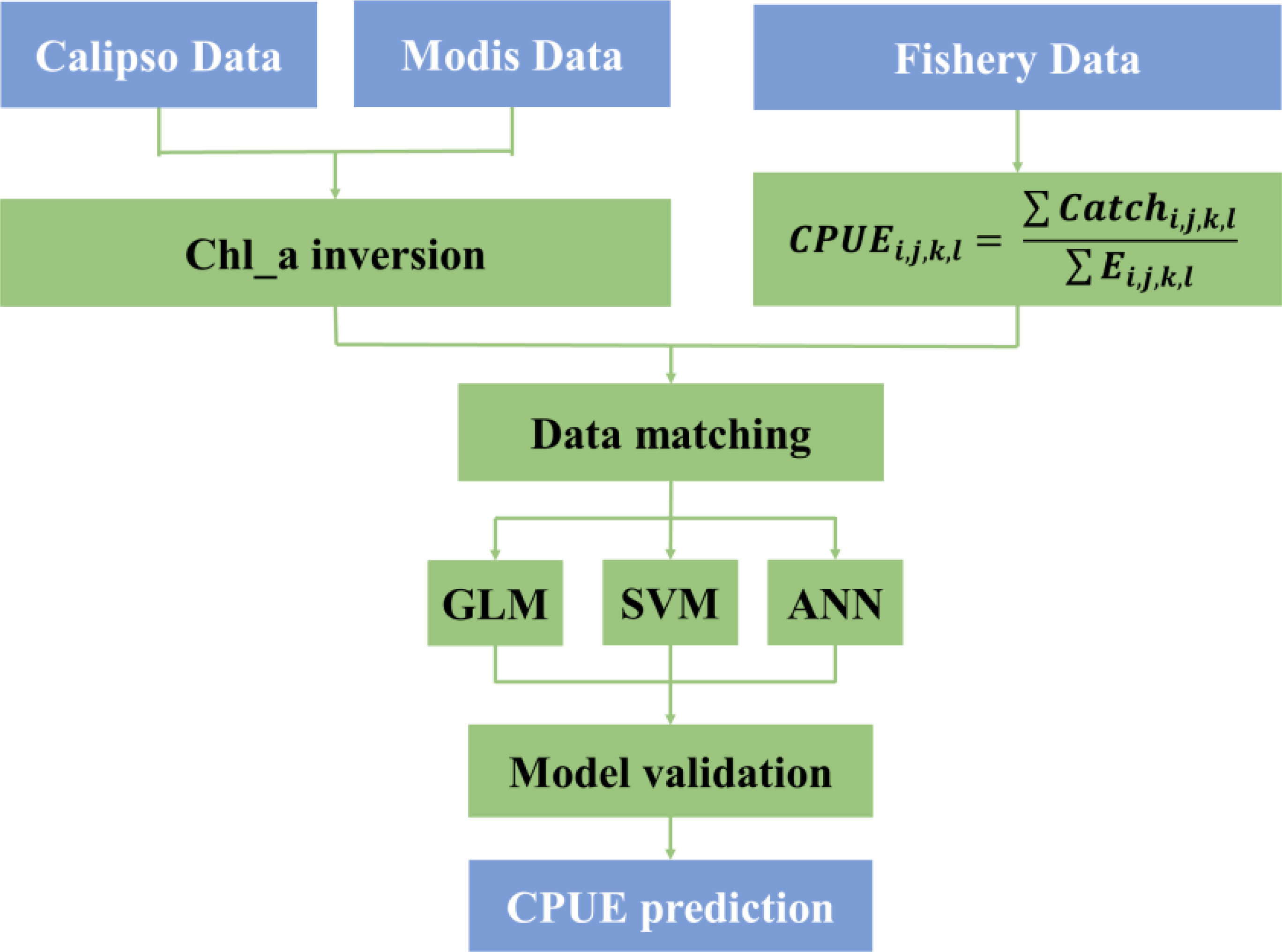
Figure 2 Flow chart of this study.

2.3.1 CALIPSO data processing for Chl_a

For CALIPSO data, the backscatter signals at 532 nm are detected by photo multiplier tubes (PMTs) through Polarization Beam Splitters (PBS). Generally, the measured signal strength is greater than the actual backscattered signal due to the transient response of the detector. Therefore, the measured signal is corrected before being processed. The corrected signal can be calculated as follows (Li et al., 2010):

$\begin{array}{ll}{\beta }^{\prime }(z)={[F]}^{-1}\beta (z)& (2)\end{array}$

where β'(z) is the real backscattered signal, β(z) is the output of the receiver and [F] is the matrix form of the transient function, which can be described as:

$\begin{array}{ll}F=\left[\begin{array}{cc}\begin{array}{ccc}F(z_2)& F(z_1)& 0\\ F(z_3)& F(z_2)& F(z_1)\end{array}& \begin{array}{cc}···& 0 \\ ···& 0 \end{array}\\ \begin{array}{ccc}···& ···& ···\\ F(z_{n+1})& F(z_n)& F(z_{n-1})\end{array}& \begin{array}{cc}···& ···\\ ···& F(z_2)\end{array}\end{array}\right]& (3)\end{array}$

In the receiver subsystems of CALIOP, the backscatter signal is separated into parallel (‖) and perpendicular (⊥) signals by PBS. However, due to nonideal characteristics, crosstalk (CT) (Pitts et al., 2018) will occur, which means that a portion of the parallel polarized signal is transmitted to the vertical channel. The effect of crosstalk can be eliminated as

$\begin{array}{ll}{\beta }_{\parallel ,\perp }=\frac{{\beta }_{\parallel ,m}}{1-CT}& (4)\end{array}$

$\begin{array}{ll}{\beta }_{\perp ,c}={\beta }_{\perp ,m}-CT\times {\beta }_{\parallel ,c}& (5)\end{array}$

where β_∥,c and β_⊥,c are corrected parallel and perpendicular signals, respectively.

After removing the effects of transient response and crosstalk in the CALIOP receiver subsystem, b_bp can be calculated from CALIOP data. The perpendicular signal is used to characterize the specific because it is difficult to extract subsurface signals from parallel channels due to interference from sea surface reflections. First, taking into account the influence of the atmosphere, the vertical-parallel ratio is used for collection (Behrenfeld et al., 2013):

$\begin{array}{ll}{\beta }_{W+}={\delta }_T\frac{{\beta }_S}{1-{\delta }_T/{\delta }_w}& (6)\end{array}$

where β_W+ is the subsurface column-integrated backscatter of the perpendicular component, δ_w is the column-integrated below-surface depolarization ratio, and β_S s the lidar surface backscatter as follows.

Then, the particulate backscatter coefficient at a 180° scattering angle is calculated:

$\begin{array}{ll}b(\pi )=2K_d{\beta }_w\frac{1+{\delta }_p}{{\delta }_p{t}^2}& (7)\end{array}$

where K_d is the ocean downwelling diffuse attenuation coefficient, t is the ocean surface transmittance and δ_p is the particulate depolarization ratio. After that, the particulate backscatter coefficient (b_bp) can be calculated based on the relationship between b(π) and b_bp:

$\begin{array}{ll}{b}_{bp}\approx \frac{b(\pi )}{0.16} \frac{532}{440}& (8)\end{array}$

Finally, Chl-a can be estimated based on the relationship between MODIS Chl_a and CALIPSO b_bp.

2.3.2 GLM

GLM is a multivariate regression model extension that assumes that the expected value of the response variable is linearly related to the explanatory variable (Hua et al., 2019). The equation of the GLM is described as:

$\begin{array}{ll}g({\mu }_i)= X_i^T\beta & (9)\end{array}$

$\begin{array}{ll}{\mu }_i=E(Y_i)& (10)\end{array}$

where g is the link function, X_i is the explanatory variable of the ith response variable, Y_i is the ith random variable, and β is the vector of the parameters.

In this paper, CPUE is assumed to follow a lognormal distribution, so the GLM is expressed as:

$\begin{array}{ll}Ln(CPU{E}_{i,j,k,l}+1)=k+{\alpha }_{1}yea{r}_i+{\alpha }_{2}mont{h}_i+{\alpha }_{3}lo{n}_i+{\alpha }_{4}la{t}_i+{\alpha }_{5}SS{T}_i+{\alpha }_{6}chl\_a_i+{\alpha }_{1}interactions+{\epsilon }_{i,j,k,l}& (11)\end{array}$

where CPUE is defined as the fishing yield per hour; interactions refer to the interaction term, which represents the interaction effect of time and space explanatory variables; α₁~a₆ are model parameters; and ε is the residual, which is assumed to have a normal distribution. In the GLM, time (year, month), space (longitude, latitude) and environment (SST, Chl_a) factors are taken as explanatory variables. Year, month, latitude, and longitude are discrete variables, and other variables are classified as continuous variables. To avoid a CPUE of 0, a constant 1 was added to CPUE before logarithmic transformation.

2.3.3 ANN

ANN have become a popular and useful software tool to model complex environmental processes. Numerous authors during the past several decades (Maier and Dandy, 2001; Suryanarayana et al., 2008; Pastore et al., 2020; Contractor and Roughan, 2021) have applied ANN techniques to characterize oceanographic processes. ANN can be used to build simple models, form different networks with different connections, and have a high degree of nonlinearity (Li et al., 2015; Sadeghi et al., 2019). They are capable of complex logical operations and nonlinear relational implementation. The overall model is given by the equation:

$\begin{array}{ll}\widehat{y}= w_{o,0}+{\sum }_{j=+1}^{o-1}f({\sum }_{i=1}^I{x}_i{w}_{j,i}+w_{j,0})w_{o,i}& (12)\end{array}$

where w_j,i denotes the weight of the connection from node j to i, o is the output node and f is the logistic function $(\frac{1}{1+e^{-x}})$. Additional details regarding the use of ANN area discussed in reference books such as Bishop (1995) and Picton (2000). Fisheries applications have been documented in Lek and Guegan (2000); Maier and Dandy (2000), and Ozesmi et al. (2006).

In this paper, Artificial neural network toolbox functions in MATLAB are used for building the network structure, training and prediction. The structure of ANN toolbox constitutes an input layer, one hidden layer with the layer size of thirty, and an output layer. The network is a two-layer feedforward network, where there is a sigmoid transfer function in the hidden layer and a linear transfer function in the output layer. The layer size value defines the number of hidden neurons. The input layer has six nodes corresponding to the input variables of environmental factors they are: year, month, latitude, longitude, CALIPSO inversed Chl_a and SST. The output layer has one node corresponding to the output variable which is the CPUE of bigeye tuna. The environmental factor data were matched with CPUE data in resolution 1°×1°. The input data was divided into three parts: 70% of the data were used for training, 15% for validation, and 15% for testing. To calculate neuron positions the layer size was 30 and the training algorithm was Bayesian regularization. The environmental factor data and CPUE data of 2008 was used for training and the model was applied to CPUE estimation from 2008 to 2015. The specific steps are: (1) match environmental factor data to CPUE based on a 1°×1° resolution; (2) calculate logarithm of environmental factor data and set as predictors, calculate logarithm of CPUE data is set as response and imported in ANN toolbox; (3) set the ratio of training data (70%), validation data (15%) and test data (15%); (4) set layer size as 30; (5) set training algorithm as Bayesian regularization; (6) train and export the model when the correlation coefficient (R) of training data in training result is higher than 0.6; and (7) environmental factor data from 2008-2015 were brought into the model for CPUE prediction. The choice of training layers and algorithms affects the training results, and the settings mentioned in this paper perform best after repeated training. Different training layers and algorithms should be set according to the specific data.

2.3.4 SVM

The SVM are data parsimonious that is developed for learning relationships in small data sets. It is an effective method to avoid local optima and has unique advantages in dealing with complex problems such as limited samples, high dimensional and nonlinear data. During the past few decades advances in SVM algorithms were developed to support the classification and regression of linear and non-linear data. Some authors have applied SVM technique to describe fisheries processes such as stream flow forecasting (Asefa et al., 2006), hydroacoustic classification of fish schools (Bosch et al., 2013) and CPUE standardization (Yang et al., 2020). The SVM performance highly relates to parameter selection and is proved perform well in seasonal flow volume predictions and CPUE standardization. SVM maps the independent variables to a high-dimensional feature space by nonlinear mapping, and finds an optimal classification surface in the high-dimensional feature space so that the error of all training samples from this optimal classification surface is minimized (Huang et al., 2004). In SVM regression (Smola and Schölkopf, 2004), the input x is first mapped onto an m-dimensional feature space using some fixed (non-linear) mapping depends of a kernel function (K). Then, the best linear separating hyper-plane in the feature space can be found (Li et al., 2015):

$\begin{array}{ll}f(x,\omega )={\sum }_{i=1}^m{\omega }_i{\varnothing }_i(x)+{\omega }_0& (13)\end{array}$

In this paper, the environmental factor data and CPUE data of 2008 were used for training and the model was applied to CPUE estimation from 2008 to 2015. The support vector machine regression model (fitrsvm) function in MATLAB was used to classify data that were not linearly separable. Followed the usage recommendations outlined by the official guide to MATLAB (2021), each predictor variable centralizes and scales by centering and dividing columns by the corresponding weighted column mean and standard deviation, and secondary sampling to select an appropriate scale factor. The ‘kfold’ for cross-validation method is 10, so that the data are randomly divided into 10 datasets, and for each dataset, the dataset used as validation data is reserved, and the 10 compact trained models are stored in the tuple vector of the cross-validation model. Gaussian function was selected as the kernel function for computing elements of the Gram matrix, which is calculated by:

$\begin{array}{ll}G(x_j,x_k)=\text{exp}(-\Vert {x_j-x_k\Vert }^2)& (14)\end{array}$

where G(x_j, x_k) is assumed an element (j,k) of the Gram matrix, where x_j and x_k are p-dimensional vectors representing the observations j and k in predictors X. In practice, the optimization problem is solved in its simpler dual form (Bottou and Lin, 2007), since this ensures that the implicit mapping only occurs in the form of the kernel G(x_j,x_k) in the optimization problem and the discriminant function (Guttormsen et al., 2016). The specific steps are: (1) match environmental factor data to CPUE based on a 1°×1° resolution; (2) choose ‘fitrsvm’ function to fit a regression Support Vector Machine (SVM); (3) environmental factor data was set as predictors, CPUE data was set as response; (4) set parameters (5) run the function and export the model; (6) environmental factor data from 2008-2015 were brought into the model for CPUE prediction. Additional details regarding the use of SVM area discussed in Steinwart and Christmann (2008).

3 Results

3.1 Results of Chl_a inversion by using CALIPSO data

CALIPSO effectively inverted the daytime and nighttime Chl_a distribution and retrieved data effectively filled in the missing parts of MODIS. Figure 3 shows the comparison of the Chl_a distribution of MODIS and CALIPSO in the study area and the distribution of CALIPSO-derived Chl_a during day and nighttime. Figure 3A shows the Chl_a data of MODIS, and it can be seen that there are significant missing data in the yellow boxes, especially near the Gulf of Guinea (0°-15°E, 6°S-6°N), where more data are missing. Near the equator, Chl_a is distributed like a tape (30°W-12°E, 6°S-5°N), and the Chl_a value is higher in the coastal areas (60°W-45°W, 0°-12°N; 17°W-15°W, 18°N-24°N; 7°E-15°E, 24°S-12°S). Figure 3B shows the Chl_a data of CALIPSO obtained by inversion using ANN based on the relationship between Chl_a of MODIS and b_bp of CALIPSO. The missing area data can be filled by the inversion of CALIPSO data, and the trend of the Chl_a distribution is roughly similar to that of MODIS. Compared with Figure 3A, the distribution of Chl_a is similar along the northeast coast of Brazil, and the distribution of Chl_a is wider offshore of Africa (0°-15°E, 24°S-6°N) with a lower concentration than that in Figure 3A. Figures 3B illustrate that the overall distribution of Chl_a is generally consistent, with a clear band distribution. Compared to the daytime (Figure 3B), Chl_a is higher at night along the northeastern coast of Brazil (45°W-30°W, 6°S-0°N), significantly lower along the coast of Mauritania (23°W-15°W, 24°S-6°N), and higher and more concentrated in the Gulf of Guinea (0°-15°E, 0°-6°N). The results of the correlation analysis show an RMSE of 0.6129 and R² of 0.8253 for daytime and nighttime Chl_a data.

FIGURE 3

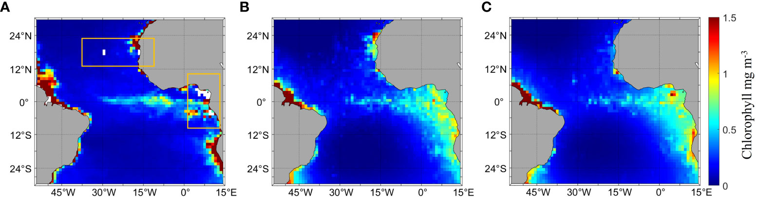
Figure 3 Comparison of the distribution of Chl_a between MODIS and CALIPSO and the circadian distribution of Chl_a in CALIPSO, (A) is the Chl_a of MODIS, the area in the yellow box is the missing data of the MODIS data, (B, C) is the Chl_a inversion by CALIPSO; (B) is the daytime distribution, (C) is the nighttime distribution.

Statistical analysis was performed on the Chl_a values of MODIS and CALIPSO, and the results are shown in Figure 4. Correlation analysis of the Chl_a from MODIS and CALIPSO values had RMSE of 0.5783 and R² of 0.5626 (see Figure 4A). From the frequency distribution of the errors (see Figure 4B), the distribution basically conforms to a normal distribution with errors ranging from -0.1 to 0.1, where the probability of 0 to 0.1 is close to 50%.

FIGURE 4

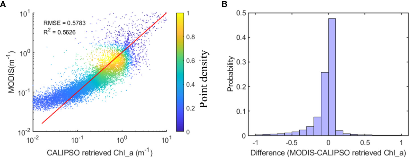
Figure 4 Statistical results of Chl_a values of MODIS and CALIPSO. (A, B) are the result of correlation analysis and frequency distribution of error, respectively.

3.2 CPUE inversion results for the Atlantic bigeye tuna

Three models (GLM, ANN, SVM) were used to model Atlantic bigeye tuna and predict CPUE. The results of the regression analysis for three models compared to the nominal CPUE are shown in Figure 5. The results indicate that ANN has the highest R² of 0.34 among the three models, followed by SVM with 0.22, and GLM with the lowest of 0.08. Because ANN and SVM are both non-linear modes, and ANN model performs better than SVM, and SVM is rarely used in CPUE researches, therefore, ANN model and GLM model are selected for further comparison in the following.

FIGURE 5

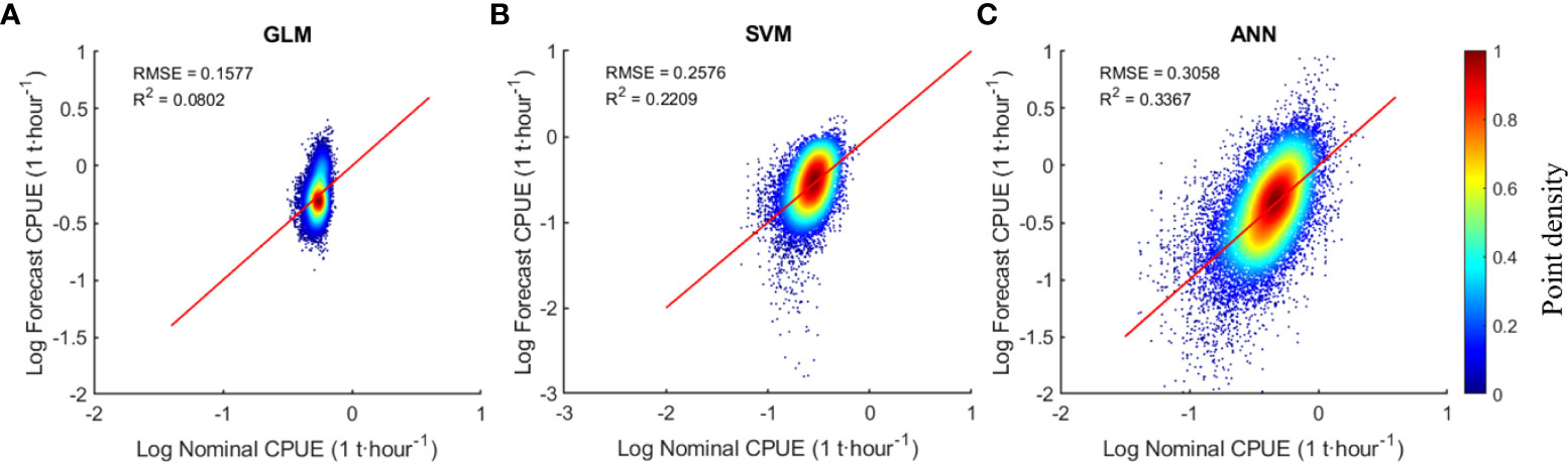
Figure 5 Comparison of regression analysis results of three models, (A–C) are GLM, SVM, ANN models respectively.

3.2.1 Comparison of the results of the GLM and ANN models

The trend in the distribution of CPUE predicted by ANN and GLM is roughly consistent with the original nominal CPUE, with relatively high predictions by GLM. Figure 6 shows the distribution of nominal CPUE and the CPUE predicted by ANN and GLM, including the cumulative CPUE values for all months from 2008 to 2015. As shown in Figure 6A, the areas with high catches are mainly located near the equator. Among them, there are two obvious high-production areas in Guinea Basin (5°W-4°W, 5°S-3°N) and the southern part of the Sierra Leone basin (13°W-8°W, 4°S-2°N), and a small high-production area in southern Cape Verde (13°W-18°W, 9°S-13°S). As seen from Figure 6B, compared to the GLM (Figure 6C), the ANN-predicted CPUE distribution is closer to the nominal CPUE distribution but with slightly lower values. For example, Figure 6B shows that there are two high-yielding areas in the southern Guinea Basin and Sierra Leone Basin, similar to Figure 6A. In Figure 6C, the GLM predicts a larger area of high production areas, mainly concentrated in 20°W to 3°E, 6°S to 4°N.

FIGURE 6

Figure 6 Distribution of the cumulative amount of CPUE in all months from 2008 to 2015. (A–C) are the CPUEs of the original measurement, ANN and GLM, respectively.

Monthly spatial distributions of nominal CPUE and CPUE predicted by ANN and GLM are shown in Figures 7, 8, 9. January to December correspond to (A) to (L), respectively, and the data of each month are the average value from 2008 to 2015. Spatially, the fishing area was mainly located south of 12°S and west of 30°W, with some high densities occurring near the equator, and the interannual variation in the spatial distribution range was generally small. The spatial location of higher abundance varied from month to month. The area of highest abundance in January (Figure 7A) was located within 14°W-3°E, 4°S-5°N. Then, the high abundance area shifted to the southeast, and in March (Figure 7C), the high abundance area appeared at 5°W-5°E, 8°S-2°N. After that, there are no distinct high abundance areas from April to July. Subsequently, in August (Figure 7H), the abundance increased at 9°W-2°E, 10°S-3°N, and a high-yield fishing area was formed that moved northward with the increase in months. Finally, in December (Figure 7L), the high abundance area was concentrated at the equator and north of the equator.

FIGURE 7

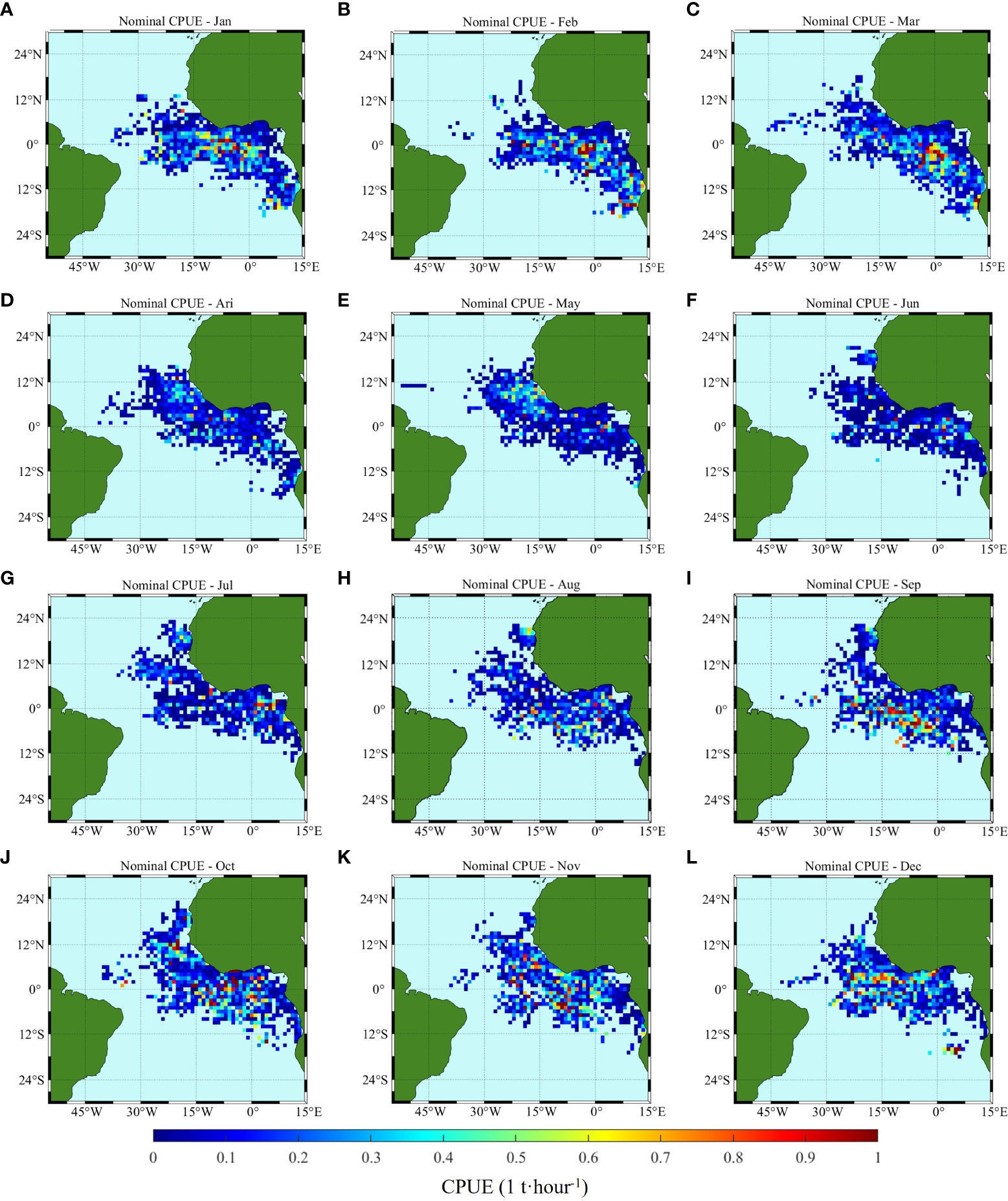
Figure 7 Climatology monthly spatial distribution of the original measured CPUE; (A–L) correspond to January to December, respectively.

FIGURE 8

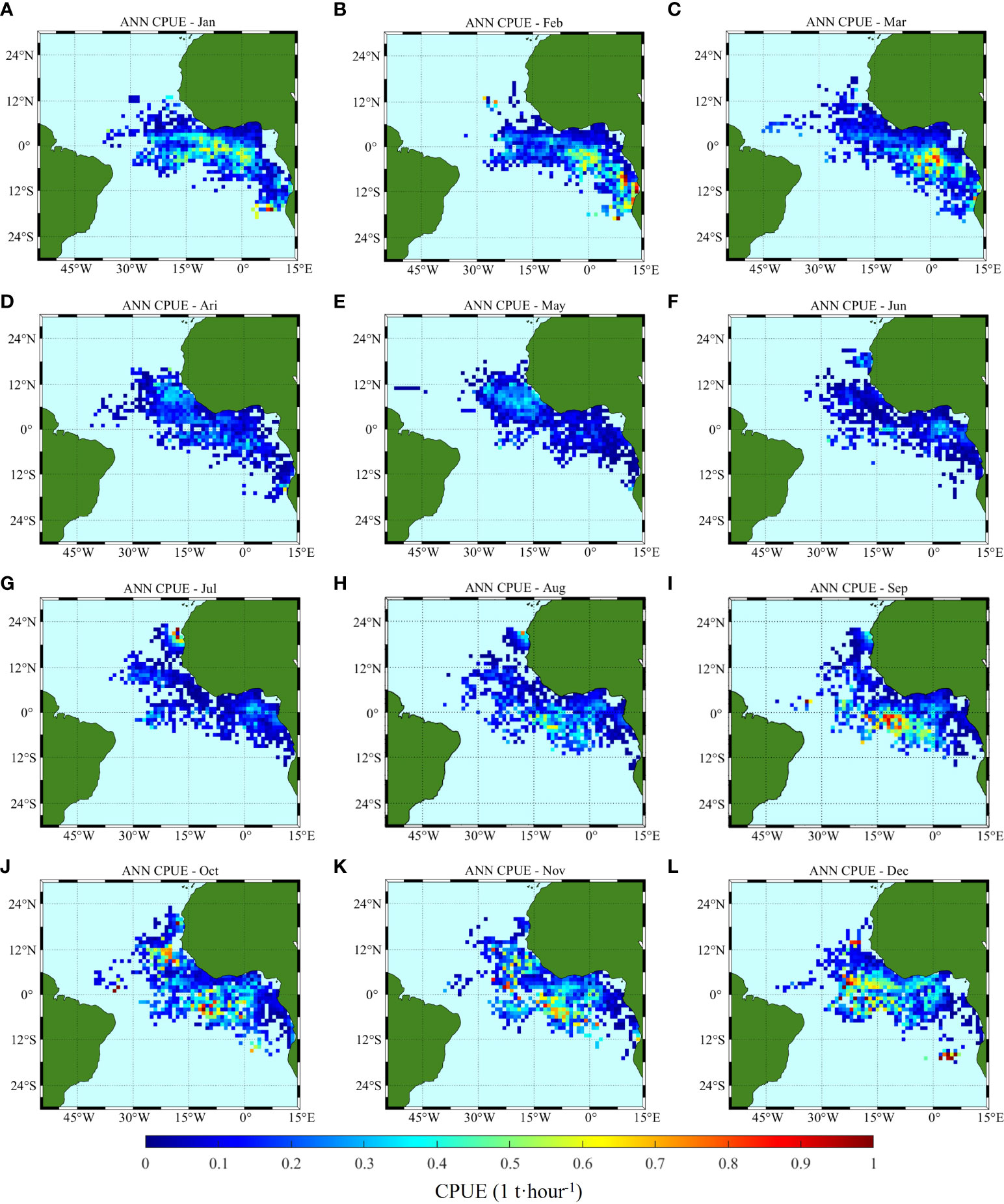
Figure 8 Climatology monthly spatial distribution of CPUE predicted by ANN, (A–L) correspond to January to December, respectively.

FIGURE 9

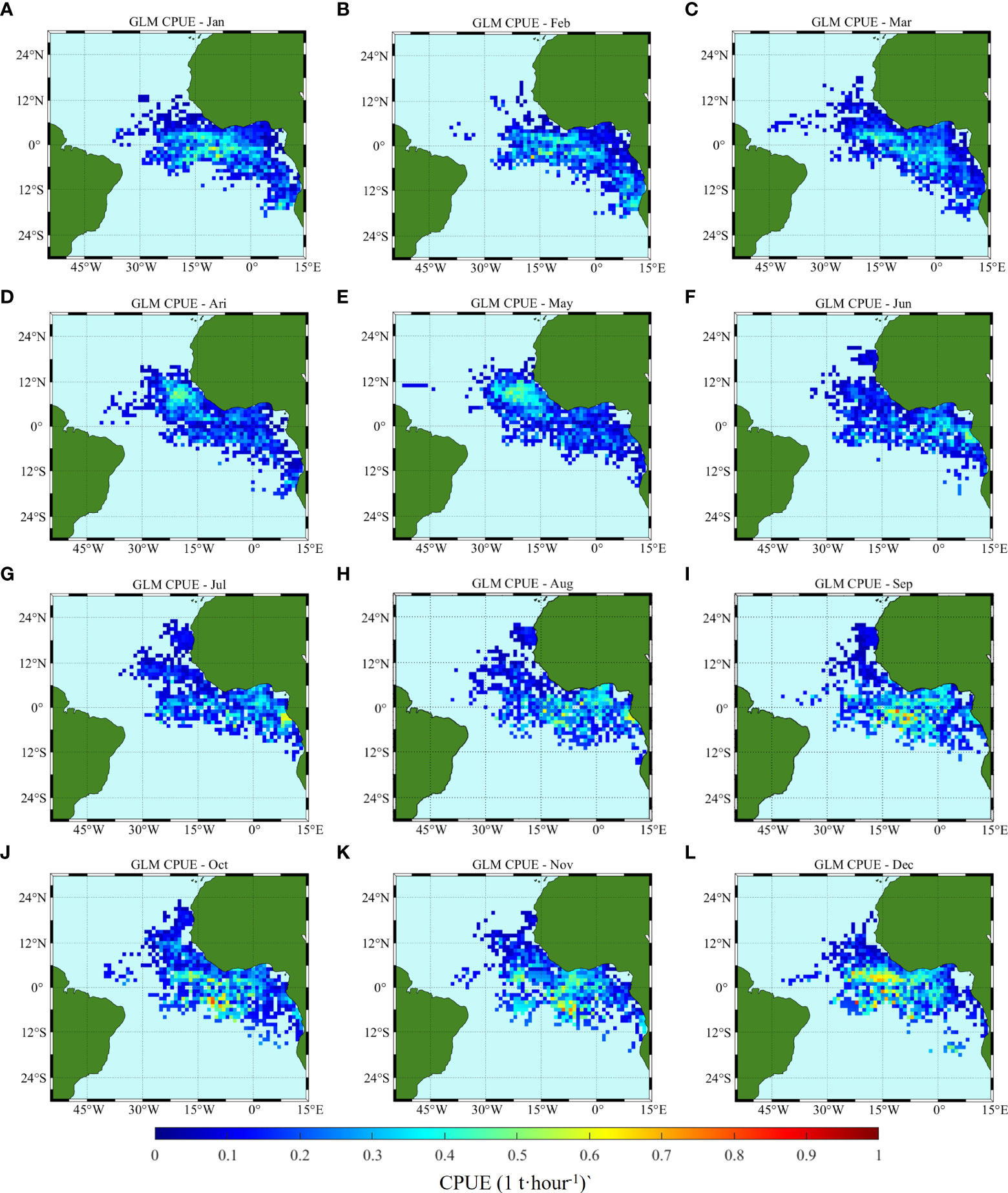
Figure 9 Climatology monthly spatial distribution of CPUE predicted by GLM, (A–L) correspond to January to December, respectively.

From the comparison of model prediction results, the distribution of CPUE predicted by ANN and GLM is consistent with the measured changes and trends. The GLM predicted values show a larger area of high production area, but the CPUE value in some areas is lower than that of ANN. GLM predicts that CPUE is lower than 0.5 t/h from January to June, and CPUE will exceed 0.6 t/h in equatorial regions after July. ANN predicts that CPUE is lower than 0.5 t/h only in March to June, and CPUE will be higher than 0.6 t/h in some regions of equatorial and southern equatorial regions in other months, even up to 1 t/h in December near the Angola basin (2°E-6°E, 18°S-16°S.).

3.2.2 Statistical analysis results

The statistical graph of CPUE accumulation calculated for different models and nominal CPUE based on different explanatory variables is shown in Figure 10. Panels (A) to (F) correspond to year, month, longitude, latitude, Chl_a, and SST, respectively. The blue line is the nominal CPUE, the green line is the CPUE predicted by ANN, and the yellow line is the CPUE predicted by GLM.

FIGURE 10

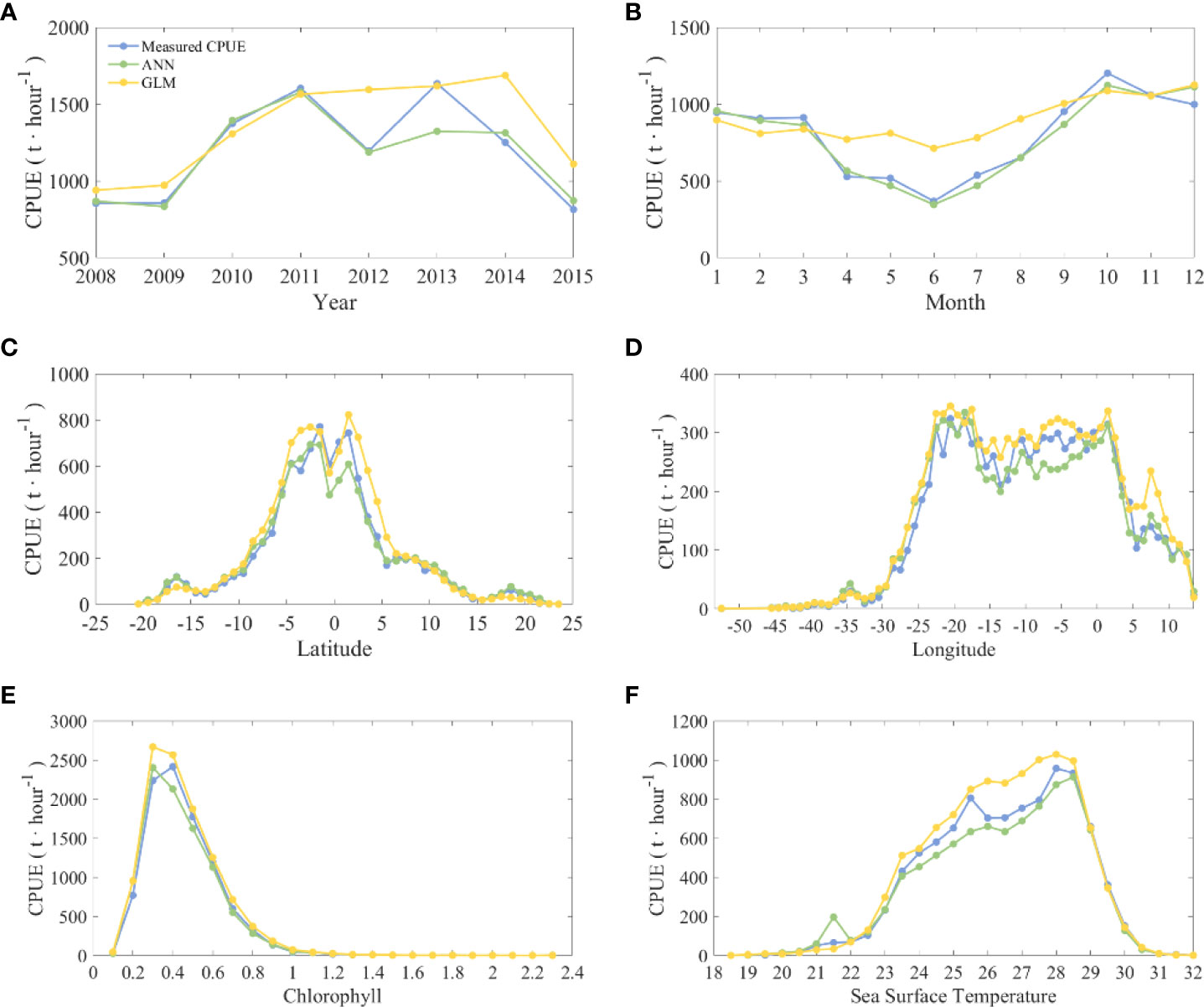
Figure 10 Statistical chart of the cumulative amount of CPUE calculated by different models and nominal CPUE according to different explanatory variables. The corresponding explanatory variables in (A–F) are year, month, latitude, longitude, chlorophyll, and sea surface temperature. The blue line is the nominal CPUE, the green line is the CPUE predicted by ANN, and the yellow line is the CPUE predicted by GLM.

Overall, the year has an effect on CPUE (Figure 10A), with a clear phase of change. The CPUE was low from 2008 to 2009 and increased significantly from 2010 to 2011. In 2012, the CPUE began to decline and rose again in the next year. After reaching its highest value in 2013, it decreased each year and finally reached its lowest value in 2015. The effect of month on CPUE shows a clear seasonal variation in CPUE (Figure 10B). CPUE was stable from January to March and then started to decline until it reached the lowest value in June. After that, CPUE began to increase and reached the highest value in October, followed by another decline in the next two months. In terms of spatial distribution (Figures 10C, D), the high values of CPUE were mainly found in the range of 25°W-5°E, 10°S-5°N, and their distribution characteristics were basically consistent with Figure 5A. In terms of environmental factors, CPUE increased as the Chl_a increased from 0.1 to 0.5 mg/m³ (Figure 10E), and CPUE peaked when the Chl_a was 0.5 mg/m³ and then decreased significantly with increasing Chl_a. When the SST (Figure 10F) was between 18 and 22°C, CPUE increased slowly with increasing SST. There was a large slope increase in CPUE from 23-28°C, while CPUE decreased briefly when SST was 25-26°C; finally, CPUE peaked when SST was 28°C and then decreased rapidly.

The model comparison results show that the ANN-predicted CPUE is closer to the nominal CPUE, and the GLM-predicted CPUE is slightly higher. The trend of ANN-predicted CPUE from 2008 to 2015 is similar to that of nominal CPUE, except for 2013, when it is much lower than the nominal CPUE. The CPUE predicted by GLM is significantly lower or higher than the nominal CPUE for all years except 2011 and 2013. The CPUE in 2012 and 2014 was significantly higher than the nominal CPUE. The monthly statistics indicate that there is no significant seasonal variation in CPUE predicted by GLM. The predicted value from January to March is slightly lower than the nominal CPUE, and from April to August, it is significantly higher than the nominal CPUE.

Table 1 shows the statistical analysis results of different explanatory variables, nominal CPUE, ANN and GLM. It can be seen that for various explanatory variables, the R² of the ANN result is higher, with the lowest R² for year at 0.8783 and R² above 0.95 for all others. In the results of the GLM, the R² is lower for year and month at 0.65 and 0.6879, respectively. When the explanatory variables are longitude and Chl_a, the R² of the GLM is higher than that of the ANN, but only by approximately 0.01.

TABLE 1

Table 1 Statistical analysis results of nominal CPUE and CPUE predicted by ANN.

3.3 CPUE inversion of Antarctic krill in the main fishing areas of Antarctica

In polar regions, both MODIS and CALIPSO are associated with outliers and missing data. CALIPSO has a higher spatial coverage than MODIS. Figure 11 shows the Chl_a distribution in the polar region, where (A) to (D) are the MODIS data and (E) to (H) are the CALIPSO inversions of Chl_a. The data for two different months are shown here, March (A, C, E, G) and September (B, D, F, H), which are chosen because, in general, on March 22, the Antarctic goes from polar day to polar night, while the Arctic goes from polar night to polar day, and in September, the Antarctic goes into polar day, while the Arctic goes into polar night. Thus, there are more Antarctic data and less Arctic data in March, while the opposite is true in September. The comparison reveals a much lower coverage of MODIS data. At the South Pole (11A) in March, there are significant gaps at the Weddell Sea (30°W to 60°W) and the Amundsen Sea (90°W to 120°W), as well as partial gaps along the coast of Queen Maud Land and Wilkes Land (0° to 150°E). In the Arctic (11C), MODIS data are almost completely missing in Hudson Bay (80°W-90°W) and Davis Strait (55°W-65°W) near southern Baffin Island. In September in Antarctica (11B), MODIS data are scarce and Chl_a is mainly distributed in 45°W-120°W and 150°W-120°E, with more data in the Arctic and higher Chl_a of about 3 m^-3 in the northern Russian coastal waters and near the Bering Strait in the eastern United States. The CALIPSO inversion of Chl_a then effectively populates the data in these regions and the Chl_a distribution is similar to that of MODIS. As can be seen from the September data, Chl_a of CALIPSO complements the region of 120°E-45°W in the Antarctic. In the Arctic, Chl_a and distribution patterns are similar to MODIS in all northern Russian seas except at the Bering Strait in the eastern United States, where Chl_a is about 3 m^-3 compared to MODIS.

FIGURE 11

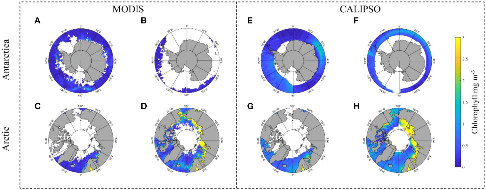
Figure 11 shows a comparison of the polar Chl_a distributions from MODIS and CALIPSO inversions. (A–D) are MODIS data, (A, B) are Antarctic; (C, D) are Arctic; (A, C) are March 2008 data (B, D) are September 2008 data; (E–H) are MODIS data, (E, F) are Antarctic; (G, H) are Arctic; (E, G) are March 2008 data (F, H) are September 2008 data; (E, G) are March 2008 data; (F, H) are September 2008 data.

Distribution of Chl_a and SST in the main fishing areas of Antarctic krill are shown in Figure 12. The fishing areas are divided into three areas according to FAO, namely, 48, 58 and 88. Chl_a is retrieved from CALIPSO data, including daytime and nighttime data. The results illustrated that the Chl_a in FA 58 (60°E-80°E, 80°S-60°S) was high and not as high in FA 88, which was dispersed. The SST increased with increasing longitude, reached the highest near the main meridian, and then decreased with increasing longitude. The SST decreases with decreasing latitude, and in FA 58, SST is higher in the latitude range of 45°S to 50°S, close to 10°C, and with the decrease in latitude, SST is approximately -1°C-3°C in the area below 60°S.

FIGURE 12

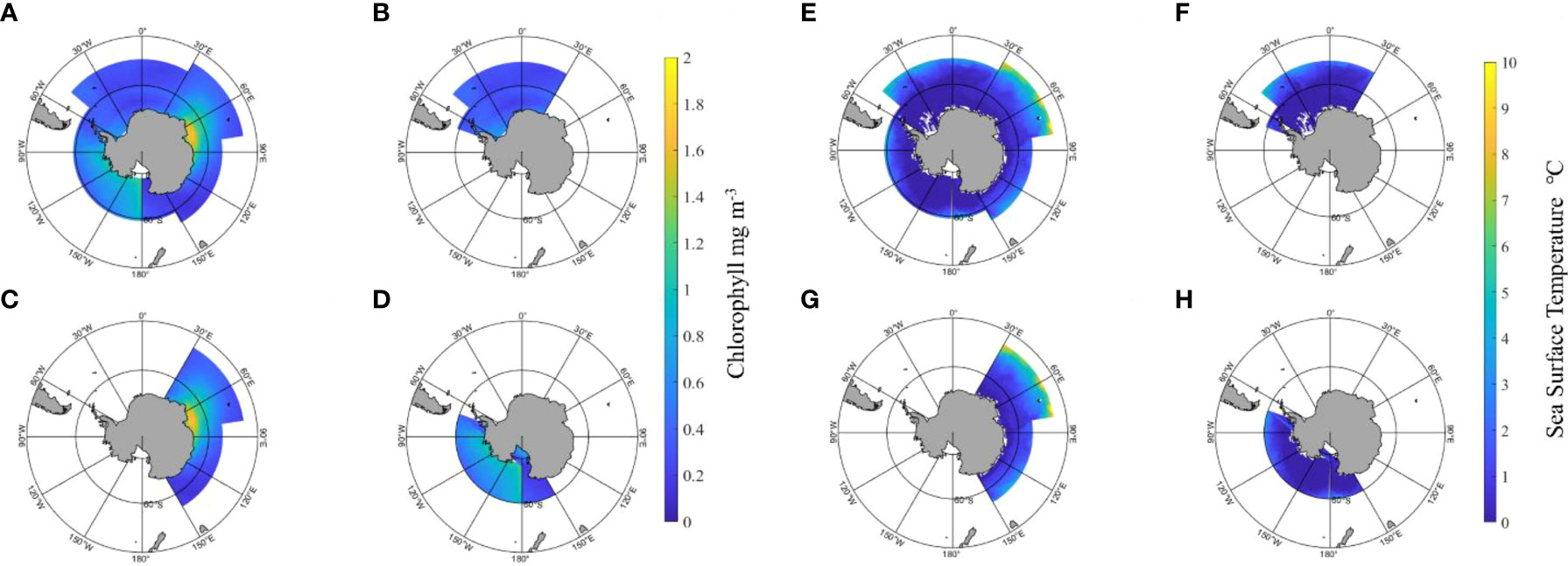
Figure 12 Distribution of chlorophyll and sea surface temperature in the main fishing areas of the polar region. (A–D) is the chlorophyll distribution, and (E–H) is the sea surface temperature distribution. (A, E) are the total fishing area, (B, F) are FA 48, (C, G) are FA 58, and (D, H) are FA 88.

The predicted CPUE and nominal CPUE for the three fishing areas were counted and compared according to different time scales (Figure 13). FA 48 has the highest CPUE (Figure 13A). In terms of annual variation, the CPUE of the FA 48 was highly variable. First, the nominal CPUE decreased from 90 tons/day (t/d) in 2008 to 60 t/d in 2009 and then increased to 100 t/d in 2010. After that, it remained at 80 t/d for three consecutive years and then increased again. Compared with the nominal CPUE, the predicted CPUE has a gentle change trend, basically maintained at 80 t/d, and began to rise in 2013. FA 58 and 88 have much lower CPUE, maintaining a nominal CPUE of 5-6 t/d in FA 58 and approximately 1.5 t/d in FA 88. The predicted CPUE for FA 58 and 88 differed from the nominal CPUE, especially for FA 88, which was higher than the nominal CPUE in all years except 2012. In terms of monthly variation, the predicted CPUE and nominal CPUE were closer for the three fishing areas (Figure 13B). Fishing area 58 showed slightly greater variability, with February and September being almost 2 t/d higher and January and November being 2 t/d lower. In FA 88, the CPUE was 0 from April to October and 6.35, 3.43 and 5.93 t/d in January, February and December, respectively.

FIGURE 13

Figure 13 shows a statistical chart of the forecast CPUE and nominal CPUE at different fishing areas at different temporal scales. (A, B) are the annual and monthly averages of CPUE in FA 48, 58 and 88, respectively. (C, D) are the annual and monthly averages of CPUE in SFA 48.1, 48.2 and 48.3, respectively.

In terms of annual variation (Figure 13C), CPUE was higher at SFA 48.1 and 48.2 than any of the other sub areas. Maximum CPUE were 161.59 t/d during 2010 in SFA 48.1 and 72.56 t/d during 2014 in SFA 48.2. The CPUE in 48.3 was generally low at approximately 30 t/d, while those in 2009 and 2010 are particularly low at 5.04 and 4.42 t/d, respectively. In terms of monthly variation (Figure 13D), SFA 48.1 and 48.2 show a similar pattern of variation, with higher CPUE values in March, April and May, followed by a gradual decrease, but differing in that in 48.1 rebounded in both October and December. In 48.3, the high CPUE values occur from June to August, reaching a maximum of 73.95 t/d in August.

The results of the correlation analysis between nominal CPUE and predicted CPUE (Figure 14) illustrate that the data have a high correlation with a R² of 0.9171, but the analysis by region reveals that only FA 48 has a high correlation of 0.7587, since FA 58 and 88 have low R² values of 0.0554 and 0.4492, respectively. The results of the correlation analysis of the three subareas showed that the correlation was high in all three areas, with the highest R² of 0.7436 for 48.2, the next highest R² of 0.7160 for 48.1, and the lowest R² of 0.6103 for 48.3.

FIGURE 14

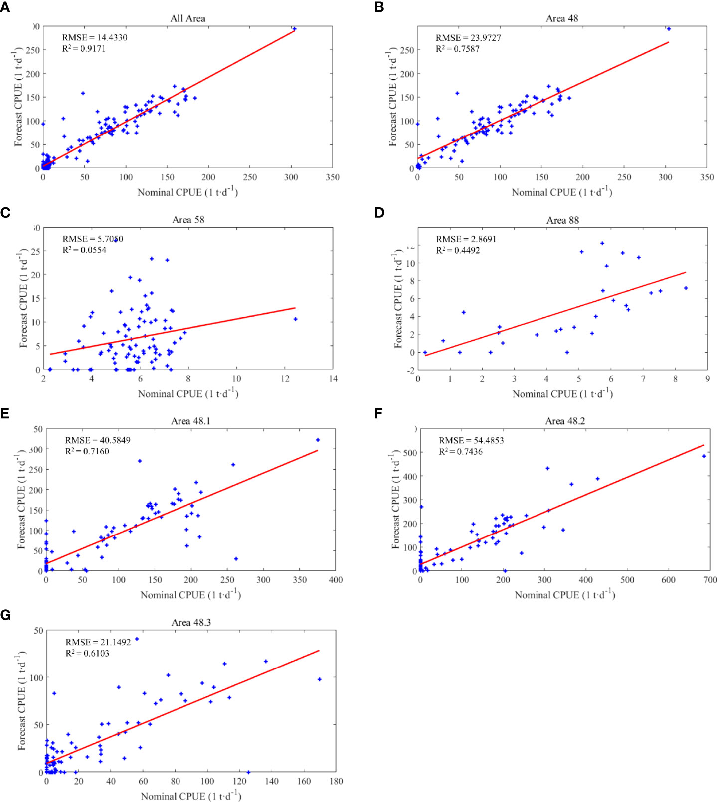
Figure 14 Results of nominal CPUE and predicted CPUE correlation analysis. (A) is the result of aggregated data for all fishing areas, (B–D) are the results for FA 48, 58, and 88, respectively; (E–G) are the results for SFA 48.1, 48.2 and 48.3.

4 Discussions

The research focused on the effects of temporal, spatial, and environmental factors impacting the CPUE of Atlantic bigeye tuna and Antarctic krill. Since the main fishing area for Antarctic krill is FA 48, studies on the relationship between the spatial and temporal distribution of Antarctic krill and environmental factors have focused on SFA 48.1, 48.2, and 48.3. Few studies were conducted in FA 58 and 88. Therefore, the discussion mainly focused on the FA 48, which can effectively understand the spatial and temporal distribution characteristics of Antarctic krill resources.

4.1 Impact of temporal factors on CPUE

This investigation evaluated temporal variability across months, seasons, and years for the period from 2008 to 2015. During this seven-year period, there was no obvious annual variation pattern between CPUE and year for bigeye tuna. Monthly variation in CPUE decreased slowly from January (946 t/h) to March (912 t/h), plunged after March, and reached the lowest point in June (369 t/h). CPUE surged after June and remained stable after reaching the highest value in October (1201 t/h). This result is consistent with past fisheries research related to Atlantic bigeye tuna. In the study of Atlantic bigeye tuna fishery, resources and environmental characteristics, Fan (2003) found that the distribution of the fishery has significant seasonal changes, and 80% of the individuals of bigeye tuna caught in the middle and late September of the year are larger than adult and medium-sized individuals after treatment. This was because the tuna is in the spawning stage, and the high catch in this stage is caused by spawning clusters.

The analysis of annual and monthly variation in Antarctic krill in different fishing areas from 2008-2015 revealed that the annual variation of CPUE was small (less than 15 t/d in FA 48, and less than 1t/d in FA 58, 88). FA 48 peaked in 2010 and then slightly decreased and continued to increase after 2013. This variation is consistent with the findings of Huang et al. (2015). The CPUE values in FA 58 and 88 are smaller, which may be influenced by the amount of biological resources (Trathan et al., 2003; Ashjian et al., 2008) and fishing techniques. The biological resources of Antarctic krill are mainly concentrated in the South Atlantic Ocean (FA 48) (Pauly et al., 2000; Nicol and Foster, 2003; Atkinson et al., 2004), and the size categories of fishing vessels used in FA 48 are 4000 to<10,000 t, while the size of fishing vessels used in FA 58 and 88 are 500 to<1000 t and 100 to<2000 t. In addition, only FA 48 and 58 are able to conduct year-round operations, while FA 88 only conducts fishing operations in January, February, March and December of each year. The Antarctic krill fishery varies seasonally and the fishing period changes accordingly. Among the three main subareas of FA 48 (Figure 13D), SFA 48.1 and 48.2 had higher monthly mean CPUE from January to April, while SFA 48.3 had higher monthly mean CPUE from May to August. This is consistent with the conclusions of international studies (Comiso and Zwally, 1984; Comiso and Steffen, 2001; Hewitt et al., 2004). In Atlantic waters (FA 48), the distribution of krill is relatively dense, mainly in the South Shetland Islands from December to April of the following year and moves offshore of South Georgia Island from May to June.

4.2 Impact of spatial factors on CPUE

The spatial distribution of bigeye tuna is generally stable among different months and years, mainly located in the Atlantic Ocean 12°S~12°N sea area. The results of the CPUE distribution of bigeye tuna can be found in Figure 10. The results are generally in agreement with the statistical analysis of the Atlantic tuna fishery by Li et al. (2013), in which Li found that the monthly mean values of CPUE in the 15°S~15°N area of the Atlantic Ocean during the breeding period were significantly higher than those in other sea areas during the same period. The spatial and temporal distribution of tuna area shows a certain pattern, forming a high-density aggregation area near the equator from January to March; gradually dividing from the concentrated piece of area into two pieces from April to September, one moving north and the other moving south; the fish aggregation area gradually moves toward the equator in October and November and converges at the breeding grounds in December, forming a cycle. The changes in the spatial distribution of tuna are related to the age composition of the tuna free school, swimming ability and the response to the spatial and temporal changes in primary productivity (Schaefer and Fuller, 2010; Fuller et al., 2015; Harper et al., 2019). In addition, the current speed and direction has a direct impact on tuna fishing production. Liu et al. (2003) found that the higher CPUE of Pacific bigeye tuna was mainly located in the medium intensity current area at the edge of the strong current zone. Current variability such as shear, and jets can affect the movement and location of fish population.

The spatial distribution of Antarctic krill can be seen in the variation in CPUE by three FA (Figure 13). Antarctic krill are mainly distributed in the South Atlantic Ocean (FA 48), while krill abundance is lower in the Southern Indian Ocean region (FA 58) (Priddle et al., 1988; Krafft et al., 2010). The Antarctic Peninsula, particularly the waters of the South Shetland Islands within the 60°S-64°S, 55°W-61°W range (SFA 48.1) and the South Orkney Islands within the 57°S-64°S, 50°W-63°W range (SFA 48.2), are the areas of maximum density distribution of Antarctic krill and the main areas of operation of the fishery (Atkinson et al., 2001; Reiss et al., 2008; Zhu et al., 2011).

4.3 Impact of environmental factors on CPUE

Analyses focused on the evaluation of CPUE as it related to changes in SST and Chl_a (observed from satellite ocean color remote sensing), which are closely associated environmental factors. CPUE of bigeye tuna was linearly correlated with SST, and CPUE was higher when the SST was high. From Figure 10, it can be seen that CPUE is higher at SST of 23.5-29°C, which is consistent with the conclusion that bigeye tuna are mostly distributed in the SST region of 24-29°C (Shen et al., 2015). Studying the relationship between CPUE and SST of Atlantic bigeye tuna, Chen (2017) found that the temperature range of Atlantic bigeye tuna fishery was 25.2-28.6°C, and the optimum temperature was 27.8-28.4°C. The CPUE of the fishery corresponded to different optimum SST in different periods, the CPUE was higher in January to April. When SST was mostly 26-27°C in May to August, the range CPUE was low. SST starts to rise from September to December, and CPUE also rises. Regarding the relationship between Chl_a and CPUE, CPUE was higher at Chl_a of 0.2-0.6 mg/m³, but its spatial distribution was not significantly correlated. The main reason for this lack of correlation may be that adult bigeye tuna are carnivorous fish and do not feed on plankton related to Chl_a. Therefore, it is difficult to judge the tuna fishery only from the Chl_a content (Fan et al., 2003). Liu et al. (2003) studied the relationship between monthly mean Chl_a content and Pacific bigeye tuna catches obtained by SeaWiFS satellite remote sensing also concluded that the correlation was low. However, some studies have shown that the Chl_a has an effect on the reproductive strategy of tuna (Block et al., 2005; Block et al., 2011). Across the world, tunas in temperate regions migrate long distances to spawn in areas where favors growth of the offspring (Muhling et al., 2017). The Atlantic bluefin tuna (Thunnus thynnus) swims from its vast feeding grounds to reproduce in areas of the Gulf of Mexico, the Mediterranean Sea (Muhling et al., 2013; Richardson et al., 2016), where primary productivity tends to be low (Ottmann et al., 2021). Tuna larvae tended to be more abundant in sites with higher water temperature, lower salinity, and lower Chl_a.

As one of the important environmental factors affecting the distribution of fishing grounds in oceanic or polar fisheries (Zhou, 2005; Ji et al., 2015), seasonal changes in SST can lead to spatial and temporal variability in the fishing grounds of target species. Based on years of research, it appears that there is a strong correlation between krill fishing grounds and SST (Priddle et al., 1988; Santa Cruz et al., 2018).

In this study, the temperature range of SST in all the sea areas of the FA 48 was -1.7-9.8°C, with an annual average value of 1.3°C; among them, the temperature ranges in SFA 48.1, 48.2 and 48.3 were -1.7-6.1°C, -1.8-5.0°C and -1.7-9.8°C, with average temperatures of 0.7, 0.5 and 2.7°C, respectively. This result is consistent with the findings of (Zhang et al. 2020). The SST range of krill fishing areas from January to June was -1.8-1.9°C, with the suitable SST in SFA 48.1, 48.2, and 48.3 being -1.8-1.9°C, -1.8-0.8°C, and -1.8-0.8°C, respectively. The suitable SST in SFA 48.1, 48.2 and 48.3 were -1.8-1.9°C, -1.8-0.8°C and 1.1-1.4°C, respectively.

The distribution of Antarctic krill was positively correlated with Chl_a (Meguro et al., 2004; Marrari et al., 2006; Marrari et al., 2008). Usually, from January to March, when the Antarctic Peninsula is in the warm season, the melting of ice floes is accompanied by a phytoplankton bloom, and krill bait is plentiful, so krill growth is metabolically vigorous and the krill population is concentrated, and fishing operations are carried out at this time with good catches.

This investigation found that Chl_a of the Antarctic in the FA 48.1, 48.2, and 48.3 were 0.07-1.57, 0.07-0.99, and 0.12-0.85 mg/m³, respectively. Atkinson et al. (2008) suggested that the Chl_a in the main habitat of Antarctic krill ranged from 0.5 to 1.0 mg/m³, and Zhang et al. (2020) concluded that the optimum Chl_a in the Antarctic was 0.13 to 0.83 mg/m³. Zhu (2012) concluded that high CPUE values for Antarctic krill in FA 48 of the northern Antarctic Peninsula usually occur in waters with Chl_a between 0 to 0.2 mg/m³.

4.4 Comparison of GLM, SVM and ANN models

The traditional GLM approach has been widely applied to standardize fishery CPUE data assuming a linear relationship between the response and explanatory variables. However, in practice, there is usually a nonlinear relationship between fish density and environmental factors (Walsh and Kleiber, 2001; Denis et al., 2002), and it is often impossible to make any assumptions about the distribution of real data. Machine learning methods, on the other hand, do not have any distributional assumptions on the data. The GLM has requirements for data structure, and the errors of both simulation and prediction of the GLM are larger under the conditions of nonlinearity and in the presence of outliers. The actual fishery production data are complex, so using the GLM for CPUE standardization of fishery data is not the optimal method. The application of SVM methods to support fisheries management has been studied infrequently. According to SCOPUS there have been less than 50 studies in the past ten years. Li et al., (2015) evaluated the performance of six candidate methods using gillnet data for Japanese Spanish mackerel collected by a fishery-dependent survey in the south of the Yellow Sea from 2006 to 2012. The analyses provided evidence that SVM can be applied as an alternative to standardize gillnet CPUE data when the proportion of zero-catch is not too large. The prediction accuracy of SVM has been discussed elsewhere (Larranaga et al., 2006; Pang et al., 2006; Verikas et al., 2011) and showed that the prediction performance of SVM varies greatly among studies. The selection of the optimal model needs to be determined based on the types of available data.

4.5 Comparison of MODIS and CALIPSO data at day and night

The advantage of CALIPSO over MODIS data is that measurements can be made at high latitudes and during nighttime (Li and Zhao, 2020). In this paper, MODIS Chl_a data were used to train the inverse Chl_a on b_bp of CALIPSO. Figure 3 shows the comparison of MODIS Chl_a and CALIPSO inversed Chl_a in the study area of Atlantic bigeye tuna. There are obvious missing parts in the MODIS data, mainly due to cloud contamination and orbital gaps (Yao et al., 2021) and spatial resolution (Guan et al., 2017). Figure 11 shows the Chl_a distribution of MODIS and CALIPSO in polar regions. It can be clearly seen that MODIS has little data in polar regions, and CALIPSO inversed Chl_a can fill the gaps in polar regions. For example, Figure 11A has a large amount of missing data west of the South Shetland Islands in Antarctica and 11C west of Greenland Island in the Arctic, and CALIPSO effectively fills the data in these areas by inversion.

5 Conclusions

In this study, a CPUE inversion method based on spaceborne lidar data was proposed. The CALIPSO-retrieved Chl_a was trained using MODIS data and applied to the standardized study of CPUE in Atlantic bigeye tuna. The GLM, SVM and ANN models were selected for modeling, and the results showed that the ANN model gave better predictions, with an R² of 0.3367 for predicted CPUE versus nominal CPUE, while the R² of the GLM and SVM were 0.0802 and 0.2209, respectively. The CPUE distribution of bigeye tuna was mainly located in the Atlantic 12°S-12°N sea area, and the spatial distribution was generally stable. The monthly variation of CPUE was obvious, which was higher in spring and winter and lowest in summer. CPUE was higher at Chl_a of 0.2-0.6 mg/m³, but its spatial distribution was not significantly correlated.

The advantages of lidar are its ability of working at night and in polar regions. CALIPSO data was trained using MODIS data and Chl_a was inversed by daytime and nighttime CALIPSO data, and ANN model was used for Antarctic krill CPUE inversion. The result illustrated that the area with high CPUE for Antarctic krill was FA 48 with an average annual CPUE of approximately 80 t/d and FA 58 and 88 with approximately 5 t/d and 2 t/d, respectively. Statistical analysis found that the correlation between predicted and nominal CPUE was higher in FA 48 among the three Antarctic fishing areas, with an R² of 0.7587. ANN was proved can be used to support polar biological resources and CPUE inversion. In addition to the methods used in this paper, there are other methods such as Regression Trees, and Random Forest, future work will apply other methods to verify the advantages and disadvantages of various methods in CPUE standardization studies.

Data availability statement

The original contributions presented in the study are included in the article/supplementary material. Further inquiries can be directed to the corresponding author.

Author contributions

ZZ performed the pre-processing of the remote sensing data. CZ conceived and designed the study. PC supervised, wrote-reviewed, and edited the manuscript. All authors contributed to the article and approved the submitted version.

Funding

This research was funded by the Key Special Project for Introduced Talents Team of Southern Marine Science and Engineering Guangdong Laboratory (GML2019ZD0602), the National Natural Science Foundation (41901305; 61991453), and the Zhejiang Natural Science Foundation (LQ19D060003), the Scientific Research Fund of the Second Institute of Oceanography, Ministry of Natural Resources (QNYC1803).

Acknowledgments

The authors are grateful to NASA Langley Research Center for providing CALIOP data through the Atmospheric Sciences Data Center (https://asdc.larc.nasa.gov/data/CALIPSO/). We thank the NASA Marine Biology Processing Group and Glob Color for also providing MODIS products (https://oceandata.sci.gsfc.nasa.gov/). We thank international commission for the conservation of Atlantic tuna (https://iccat.int/en/) for providing tuna production data. We thank the Commission for the Conservation of Antarctic Marine Living Resources (https://www.ccamlr.org/) for providing Antarctic krill production data. We thank reviewers for their suggestions, which significantly improved the presentation of the paper.

Conflict of interest

The authors declare that the research was conducted in the absence of any commercial or financial relationships that could be construed as a potential conflict of interest.

Publisher’s note

All claims expressed in this article are solely those of the authors and do not necessarily represent those of their affiliated organizations, or those of the publisher, the editors and the reviewers. Any product that may be evaluated in this article, or claim that may be made by its manufacturer, is not guaranteed or endorsed by the publisher.

References

Asefa T., Kemblowski M., Mckee M., Khalil A. (2006). Multitime scale stream flow predictions: The support vector machines approace. J. Hydrology 318 (1-4), 7–16. doi: 10.1016/j.jhydrol.2005.06.001

CrossRef Full Text | Google Scholar

Ashjian C., Davis C., Gallager S., Wiebe P., Lawson G. (2008). Distribution of larval krill and zooplankton in association with hydrography in Marguerite bay, Antarctic peninsula, in austral fall and winter 2001 described using the video plankton recorder. Deep-sea Res. Part Ii-topical Stud. Oceanography - DEEP-SEA Res. PT II-TOP ST OCE 55 (3-4), 455–471. doi: 10.1016/j.dsr2.2007.11.016

CrossRef Full Text | Google Scholar

Atkinson A., Siegel V., Pakhomov E., Rothery P. (2004). Long-term decline in krill stock and increase in salps within the southern ocean. Nature 432, 100–103. doi: 10.1038/nature02996

PubMed Abstract | CrossRef Full Text | Google Scholar

Atkinson A., Siegel V., Pakhomov E., Rothery P., Loeb V., Ross R., et al. (2008). Oceanic circumpolar habitats of Antarctic krill. Mar. Ecol. Prog. Ser. 362, 1–23. doi: 10.3354/meps07498

CrossRef Full Text | Google Scholar

Atkinson A., Whitehouse M., Priddle J., Cripps G., Ward P., Brandon M. (2001). South Georgia, Antarctica: A productive, cold water, pelagic ecosystem. Mar. Ecol. Prog. Ser. 216, 279–308. doi: 10.3354/meps216279

CrossRef Full Text | Google Scholar

Babin M., Arrigo K. R., Bélanger S., Forget M.-H., IOCCG. (2015). Ocean colour remote sensing in polar seas (Canada: International Ocean Colour Coordinating Group).

Google Scholar

Behrenfeld M., Hu Y., Hostetler C., Dall'olmo G., Rodier S., Hair J., et al. (2013). Space-based lidar measurements of global ocean carbon stocks. Geophysical Res. Lett. 40, 4355–4360. doi: 10.1002/grl.50816

CrossRef Full Text | Google Scholar

Betz E. (2015). Hacking a climate satellite to see beneath the ocean's surface. Eos 96. doi: 10.1029/2015EO030183

CrossRef Full Text | Google Scholar

Bigelow K., Boggs C., He X. I. (1999). Environmental effects on swordfish and blue shark catch rates in the US north pacific longline fishery. Fisheries Oceanography 8 (3), 178–198. doi: 10.1046/j.1365-2419.1999.00105.x

CrossRef Full Text | Google Scholar

Bishop C. M. (1995). Neural networks for pattern recognition (Oxford University Press, USA: Clarendon Press).

Google Scholar

Block B., Jonsen I., Jorgensen S., Winship A., Shaffer S., Bograd S., et al. (2011). Tracking apex marine predator movements in a dynamic ocean. Nature 475, 86–90. doi: 10.1038/nature10082

PubMed Abstract | CrossRef Full Text | Google Scholar

Block B., Teo S., Walli A., Boustany A., Stokesbury M., Farwell C., et al. (2005). Electronic tagging and population structure of Atlantic bluefin tuna. Nature 434, 1121–1127. doi: 10.1038/nature03463

PubMed Abstract | CrossRef Full Text | Google Scholar

Bosch P., Lópeza J., Héctor R., Robotham H. (2013). Support vector machine under uncertainty: An application for hydroacoustic classification of fish-schools in Chile. Expert Syst. Appl. 40 (10), 4029–4034. doi: 10.1016/j.eswa.2013.01.006

CrossRef Full Text | Google Scholar

Bottou L., Lin C. J. (2007). Support vector machine solvers. Large scale kernel machines, 301–320. doi: 10.7551/mitpress/7496.003.0003

CrossRef Full Text | Google Scholar

CCAMLR (2017). Map of the CAMLR Convention Area. Last updated October 2017. Available at: www.ccamlr.org/node/86816.

Google Scholar

Chen L. (2017). Spatical-temporal distribution of catch rate and relations to marine environment for the bigeye tuna (Thunnus obesus) in Atlantic ocean. Shanghai Ocean Univ. 31.

Google Scholar

Chen X. J., Liu B. L., Chen Y. (2008). A review of the development of Chinese distant-water squid jigging fisheries. Fisheries Res. 89 (3), 211–221. doi: 10.1016/j.fishres.2007.10.012

CrossRef Full Text | Google Scholar

Chen H., Li J., Yang W., Li D., Wang J. (2011). The habitat suitability index of feeding migration stock of small yellow croaker pseudosciaena polyactis in the East Sea and the yellow Sea. J. Dalian Ocean Univ. 26 (4), 348–351. doi: 10.3969/j.issn.1000-9957.2011.04.012

CrossRef Full Text | Google Scholar

Chen P., Mao Z., Zhang Z., Liu H., Pan D. (2019). Detecting subsurface phytoplankton layer in qiandao lake using shipborne lidar. Optics Express 28 (1), 558–569. doi: 10.1364/OE.381617

CrossRef Full Text | Google Scholar

Churnside J. H. (1999). Can we see fish from an airplane? In Airborne and in-water underwater imaging (Gilbert G. D. ed.), p. 45–48. Proc. SPIE (Society of Photo-Optical Instrumentation Engineers) (Bellingham, WA, SPIE). doi: 10.1117/12.366482

CrossRef Full Text | Google Scholar

Churnside J. (2007). LIDAR detection of plankton in the ocean. IEEE Int. Geosci. Remote Sens. Symposium, 3174–3177. doi: 10.1109/IGARSS.2007.4423519

CrossRef Full Text | Google Scholar

Churnside J. (2013). Review of profiling oceanographic lidar. Optical Eng. 53, 51405. doi: 10.1117/1.OE.53.5.051405

CrossRef Full Text | Google Scholar

Churnside J., Donaghay P. (2009). Thin scattering layers observed by airborne lidar. Ices J. Mar. Sci. - ICES J. Mar. Sci. 66 (4), 778–789. doi: 10.1093/icesjms/fsp029

CrossRef Full Text | Google Scholar

Churnside J., Hanan D., Hanan Z., Marchbanks R. (2011). Lidar as a tool for fisheries management. Proc. SPIE 8159 (1), 81590J. doi: 10.1117/12.892560

CrossRef Full Text | Google Scholar

Comiso J. C., Steffen K. (2001). Studies of Antarctic sea ice concentrations from satellite data and their applications. J. Geophysical Research: Oceans 106 (C12), 31361–31385. doi: 10.1029/2001JC000823

CrossRef Full Text | Google Scholar

Comiso J., Zwally H. (1984). Concentration gradients and growth/decay characteristics of seasonal sea ice cover. J. Geophysical Res. 89 (C5), 8081–8103. doi: 10.1029/JC089iC05p08081

CrossRef Full Text | Google Scholar

Contractor S., Roughan M. (2021). Efficacy of feedforward and LSTM neural networks at predicting and gap filling coastal ocean timeseries: Oxygen, nutrients, and temperature. Front. Mar. Sci. 8. doi: 10.3389/fmars.2021.637759

CrossRef Full Text | Google Scholar

Denis V., Lejeune J., Denis J., Lejeune V., Spatio J., Robin J.-P. (2002). Spatio-temporal analysis of commercial trawler data using general additive models: patterns of loliginid squid abundance in the north-east Atlantic. ICES J. Mar. Sci. 59 (3), 633–648. doi: 10.1006/jmsc.2001.1178

CrossRef Full Text | Google Scholar

Erisman B., Allen L., Claisse J., Pondella D., Miller E., Murray J., et al. (2011). The illusion of plenty: Hyperstability masks collapses in two recreational fisheries that target fish spawning aggregations. Can. J. Fisheries Aquat. Sci. 68 (10), 1705–1716. doi: 10.1139/f2011-090

CrossRef Full Text | Google Scholar

Fan W., Shen Q. X., Lin S. M. (2003). Study on resource environment and fishing-ground of Atlantic bigeye tuna. Acta Oceanologica Sin. 25 (10), 167–176.

Google Scholar

Fuller D., Schaefer K., Hampton J., Caillot S., Leroy B., Itano D. (2015). Vertical movements, behavior, and habitat of bigeye tuna (Thunnus obesus) in the equatorial central pacific ocean. Fisheries Res. 172, 57–70. doi: 10.1016/j.fishres.2015.06.024

CrossRef Full Text | Google Scholar

Guan W. J., Gao F., Chen X. J. (2017). Review of the applications of satellite remote sensing in the exploitation,management and protection of marine fisheries resources. J. Shanghai Ocean Univ. 26 (3), 440–449. doi: 10.12024/jsou.20160701826

CrossRef Full Text | Google Scholar

Guan W. J., Tian S. Q., Wang X. F., Zhu J. F., Chen X. J. (2014). A review of methods and model selection for standardizing CPUE. J. Fishery Sci. China 21 (4), 852–862. doi: 10.3724/SP.J.1118.2014.00852

CrossRef Full Text | Google Scholar

Guttormsen E., Toldnes B., Bondø M., Eilertsen A, Gravdahl J. T., Mathiassen J. R., et al. (2016). A machine vision system for robust sorting of herring fractions. Food Bioprocess Technol. 9, 1893–1900. doi: 10.1007/s11947-016-1774-2

CrossRef Full Text | Google Scholar

Harley S., Myers R., Dunn A. (2001). Is catch-per-Unit-Effort proportional to abundance. Can. J. Fisheries Aquat. Sci. 58 (9), 1760–1772. doi: 10.1139/cjfas-58-9-1760

CrossRef Full Text | Google Scholar

Harper L., Buxton A., Rees H., Bruce K., Brys R., Halfmaerten D., et al. (2019). Prospects and challenges of environmental DNA (eDNA) monitoring in freshwater ponds. Hydrobiologia 826, 25–41. doi: 10.1007/s10750-018-3750-5

CrossRef Full Text | Google Scholar

Hewitt R., Watkins J., Naganobu M., Sushin V., Brierley A., Demer D., et al. (2004). Biomass of Antarctic krill in the Scotia Sea in January/February 2000 and its use in revising an estimate of precautionary yield. Deep Sea Res. Part II: Topical Stud. Oceanography 51 (12-13), 1215–1236. doi: 10.1016/j.dsr2.2004.06.011

CrossRef Full Text | Google Scholar

Huang Z., Chen H.-C., Hsu C.-J., Chen W.-H., Wu S. (2004). Credit rating analysis with support vector machines and neural networks: A market comparative study. Decision Support Syst. 37 (4), 543–558. doi: 10.1016/S0167-9236(03)00086-1

CrossRef Full Text | Google Scholar

Huang H. L., Chen X. Z., Liu J., Li Z. L., Wu Y., Yang J. L., et al. (2015). Analysis of the status and trend of the antarctic krill fishery. Chin. J. Polar Res. 27 (1), 25–30. doi: 10.13679/j.jdyj.2015.1.025

CrossRef Full Text | Google Scholar

Hua C., Zhu Q., Shi C., Liu Y. (2019). Comparative analysis of CPUE standardization of Chinese pacific saury (Cololabis saira) fishery based on GLM and GAM. Acta Oceanologica Sin. 38 (10), 100–110. doi: 10.1007/s13131-019-1486-3

CrossRef Full Text | Google Scholar

Irish J. L., Mcclung J. K., Lillycrop W. (2000). Airborne lidar bathymetry : The SHOALS system. Bull. Int. Navigation Assoc. 43-53. doi: 10.1016/S0924-2716(99)00003-9

CrossRef Full Text | Google Scholar

Ji S., Zhou W., Cheng T., Chen G. (2015). On the forecast and analysis of fishing grounds in the open south China Sea. Fishery Inf. Strategy 30 (2), 98–105. doi: 10.13233/j.cnki.fishis.2015.02.004

CrossRef Full Text | Google Scholar

Kamei G., Felix J., Shenoy L., Shukla S., Devi H. (2014). Application of remote sensing in fisheries: Role of potential fishing zone advisories 10, 175–186. doi: 10.1007/978-3-319-01689-4_10

CrossRef Full Text | Google Scholar

Kim M.-H., Omar A., Tackett J., Vaughan M., Winker D., Trepte C., et al. (2018). The CALIPSO version 4 automated aerosol classification and lidar ratio selection algorithm. Atmospheric Measurement Techniques 11 (11), 6107–6135. doi: 10.5194/amt-11-6107-2018

PubMed Abstract | CrossRef Full Text | Google Scholar

Krafft B., Melle W., Knutsen T., Bagøien E., Broms C., Ellertsen B., et al. (2010). Distribution and demography of Antarctic krill in the southeast Atlantic sector of the southern ocean during the austral summer 2008. Polar Biol. 33, 957–968. doi: 10.1007/s00300-010-0774-3

CrossRef Full Text | Google Scholar

Larranaga P., Calvo B., Santana R., Bielza C., Galdiano J., Inza I., et al. (2006). Machine learning in bioinformatics. Briefings Bioinf. 7 (1), 86–112. doi: 10.1093/bib/bbk007

CrossRef Full Text | Google Scholar

Lek S., Guegan J. F. (2000). Artificial neural networks: application to ecology and evolution (Berlin, Heidelberg: Springer).

Google Scholar

Li J., Hu Y. X., Huang J. B., Stamnes K., Yi H. L. (2010). A new method for retrieval of the extinction coefficient of water clouds by using the tail of the CALIOP signal. Atmospheric Chem. Phys. Discussions 10 (11), 2903–2916. doi: 10.5194/acpd-10-28151-2010

CrossRef Full Text | Google Scholar

Liu H., Chen P., Mao Z. H., Pan D. L., He Y. (2018). Subsurface plankton layers observed from airborne lidar in sanya bay, south China Sea. Optics Express 26 (22), 29134–29147. doi: 10.1364/OE.26.029134

PubMed Abstract | CrossRef Full Text | Google Scholar

Liu C. T., Nan C. H., Ho C. R., Kuo N. J., Mingkuang H., Tseng R.-S. (2003). Application of satellite remote sensing on the tuna fishery of Eastern tropical pacific. Int. Assoc. Geodesy Symp. 126, 175–183. doi: 10.1007/978-3-642-18861-9_21

CrossRef Full Text | Google Scholar

Li Z. L., Wang L., Liu J., Liu Q., Huang H. L. (2013). Geostatistical analysis of tuna ( Thunnus obesus ) longline fishing grounds in the Atlantic ocean. J. Fishery Sci. China 20 (1), 198–204. doi: 10.3724/SP.J.1118.2013.00198

CrossRef Full Text | Google Scholar

Li Z. G., Ye Z. J., Wan R., Zhang C. (2015). Model selection between traditional and popular methods for standardizing catch rates of target species: A case study of Japanese Spanish mackerel in the gillnet fishery. Fisheries Res. 161, 312–319. doi: 10.1016/j.fishres.2014.08.021

CrossRef Full Text | Google Scholar

Li X. L., Zhao C. F. (2020). Application and development of lidar to detect the vertical distribution of marine materials. Infrared Laser Eng. 9 (S02), 20200381. doi: 10.3788/irla20200381

CrossRef Full Text | Google Scholar

Lu X. M., Hu Y. X., Trepte C., Zeng S., Churnside J. (2014). Ocean subsurface studies with the CALIPSO spaceborne lidar. J. Geophysical Research: Oceans 119 (7), 4305–4317. doi: 10.1002/2014JC009970

CrossRef Full Text | Google Scholar

Lu X. M., Hu Y. X., Yang Y. K., Bontempi P., Omar A., Baize R. (2020). Antarctic Spring ice-edge blooms observed from space by ICESat-2. Remote Sens. Environ. 245, 111827. doi: 10.1016/j.rse.2020.111827

CrossRef Full Text | Google Scholar

Lu X., Hu Y., Yang Y., Neumann T., Omar A., Baize R., et al. (2021). New ocean subsurface optical properties from space lidars: CALIOP/CALIPSO and ATLAS/ICESat-2. Earth Space Sci. 8, e2021EA001839. doi: 10.1029/2021EA001839

CrossRef Full Text | Google Scholar

Maier H. R., Dandy G. C. (2000). Neural networks for the prediction and forecasting of water resources variables: A review of modelling issues and applications. Environ. Model. Software 15 (1), 101–124. doi: 10.1016/S1364-8152(99)00007-9

CrossRef Full Text | Google Scholar

Maier H. R., Dandy G. C. (2001). Neural network based modelling of environmental variables: A systematic approach, mathematical and computer modelling. Mathematical and Computer Modelling 33, 6-7, 669–682. doi: 10.1016/S0895-7177(00)00271-5

CrossRef Full Text | Google Scholar

Marrari M., Daly K., Hu C. (2008). Spatial and temporal variability of SeaWiFS chlorophyll a distributions west of the Antarctic peninsula: Implications for krill production. Deep Sea Res. Part II: Topical Stud. Oceanography 55 (3-4), 377–392. doi: 10.1016/j.dsr2.2007.11.011

CrossRef Full Text | Google Scholar

Marrari M., Hu C., Daly K. (2006). Validation of SeaWiFS chlorophyll a concentrations in the southern ocean: A revisit. Remote Sens. Environ. 105 (4), 367–375. doi: 10.1016/j.rse.2006.07.008

CrossRef Full Text | Google Scholar

MATLAB (2021). The MathWorks inc (Natick, Massachusetts, United States: MathWorks).

Google Scholar

Maunder M., Langley A. (2004). Integrating the standardization of catch-per-unit-of-effort into stock assessment models: Testing a population dynamics model and using multiple data types. Fisheries Res. 70 (2-3), 389–395. doi: 10.1016/j.fishres.2004.08.015

CrossRef Full Text | Google Scholar

Maunder M., Punt A. (2004). Standardizing catch and effort data: A review of recent approaches. Fisheries Res. 70 (2-3), 141–159. doi: 10.1016/j.fishres.2004.08.002

CrossRef Full Text | Google Scholar

Meguro H., Toba Y., Murakami H., Kimura N. (2004). Simultaneous remote sensing of chlorophyll, sea ice and sea surface temperature in the Antarctic waters with special reference to the primary production from ice algae. Adv. Space Res. - Adv. SPACE Res. 33 (7), 1168–1172. doi: 10.1016/S0273-1177(03)00368-5

CrossRef Full Text | Google Scholar

Mountrakis G., Im J., Ogole C. (2011). Support vector machines in remote sensing: A review. ISPRS J. Photogrammetry Remote Sens. 66 (3), 247–259. doi: 10.1016/j.isprsjprs.2010.11.001

CrossRef Full Text | Google Scholar

Muhling B., Lamkin J., Alemany F., García A., Farley J., Ingram J. G., et al. (2017). Reproduction and larval biology in tunas, and the importance of restricted area spawning grounds. Rev. Fish Biol. Fisheries 27, 697–732. doi: 10.1007/s11160-017-9471-4

CrossRef Full Text | Google Scholar

Muhling B., Reglero P., Ciannelli L., Alvarez-Berastegui D., Alemany F., Lamkin J., et al. (2013). Comparison between environmental characteristics of larval bluefin tuna thunnus thynnus habitat in the gulf of Mexico and western Mediterranean Sea. Mar. Ecol. Prog. Ser. 486, 257–276. doi: 10.3354/meps10397

CrossRef Full Text | Google Scholar

Nicol S., Foster J. (2003). Recent trends in the fishery for Antarctic krill. Aquat. Living Resour. 16 (1), 42–45. doi: 10.1016/S0990-7440(03)00004-4

CrossRef Full Text | Google Scholar

Ochi D., Matsumoto T., Satoh K., Okamoto H. (2014). Japanese Longline CPUE for bigeye tuna in the Indian ocean standardized by GLM. IOTC-2017-WPTT 19–28

Google Scholar

Ottmann D., Fiksen Ø., Martín M., Alemany F., Prieto L., Alvarez-Berastegui D., et al. (2021). Spawning site distribution of a bluefin tuna reduces jellyfish predation on early life stages. Limnology Oceanography 66 (10), 3669–3681. doi: 10.1002/lno.11908

CrossRef Full Text | Google Scholar

Ozesmi S. L., Tan C. O., Ozesmi U. (2006). Methodological issues in building, training, and testing artificial neural networks in ecological applications. Ecol. Model. 195 (1-2), 83–93. doi: 10.1016/j.ecolmodel.2005.11.012

CrossRef Full Text | Google Scholar

Pang H., Lin A., Holford M., Enerson B., Lu B., Lawton M., et al. (2006). Pathway analysis using random forests classification and regression. Bioinf. (Oxford England) 22 (16), 2028–2036. doi: 10.1093/bioinformatics/btl344

CrossRef Full Text | Google Scholar

Pastore V. P., Zimmerman T. G., Biswas S. K., Bianco S. (2020). Annotation-free learning of plankton for classification and anomaly detection. Sci. Rep. 10, 12142. doi: 10.1038/s41598-020-68662-3

PubMed Abstract | CrossRef Full Text | Google Scholar

Pauly T., Nicol S., Higginbottom I., Hosie G., Kitchener J. (2000). Distribution and abundance of Antarctic krill (Euphausia superba) off East Antarctica (80-150 °E) during the austral summer of 1995/1996. Deep Sea Res. Part II: Topical Stud. Oceanography 47 (12-13), 2465–2488. doi: 10.1016/S0967-0645(00)00032-1

CrossRef Full Text | Google Scholar

Perez J., Alvarez M., Heikkonen J., Guillen J., Barbas T. (2013). The efficiency of using remote sensing for fisheries enforcement: Application to the Mediterranean bluefin tuna fishery. Fisheries Res. 147, 24–31. doi: 10.1016/j.fishres.2013.04.008

CrossRef Full Text | Google Scholar

Picton P. (2000). Neural networks (Palgrave Macmillan).

Google Scholar

Pitts M., Poole L., Gonzalez R. (2018). Polar stratospheric cloud climatology based on CALIPSO spaceborne lidar measurements from 2006–2017. Atmospheric Chem. Phys. Discussions 18 (15), 10881–10913. doi: 10.5194/acp-2018-234

CrossRef Full Text | Google Scholar

Priddle J., Croxall J., Everson I., Heywood R., Murphy E., Prince P., et al. (1988). Large-Scale fluctuations in distribution and abundance of krill — A discussion of possible causes. Antarctic Ocean and Resources Variability 169–182. doi: 10.1007/978-3-642-73724-4_14

CrossRef Full Text | Google Scholar

Reiss C., Cossio A., Loeb V., Demer D. (2008). Variations in the biomass of Antarctic krill (Euphausia superba) around the south Shetland islands 1996-2006. Ices J. Mar. Sci. - ICES J. Mar. Sci. 65 (4), 497–508. doi: 10.1093/icesjms/fsn033

CrossRef Full Text | Google Scholar

Richardson D., Marancik K., Guyon J., Lutcavage M., Galuardi B., Lam C., et al. (2016). Discovery of a spawning ground reveals diverse migration strategies in Atlantic bluefin tuna ( thunnus thynnus ). Proc. Natl. Acad. Sci. 113 (12), 3299–3304. doi: 10.1073/pnas.1525636113

CrossRef Full Text | Google Scholar

Rodríguez-Marín E., Arrizabalaga H., Ortiz M., Rodríguez-Cabello C., Moreno G., Kell L. (2003). Standardization of bluefin tuna, thunnus thynnus, catch per unit effort in the baitboat fishery of the bay of Biscay (Eastern Atlantic). ICES J. Mar. Sci. 60 (6), 1216–1231. doi: 10.1016/S1054-3139(03)00139-5

CrossRef Full Text | Google Scholar

Sadeghi M., Asanjan A. A., Faridzad M., Nguyen P., Hsu K., Sorooshian S., et al. (2019). PERSIANN-CNN: Precipitation estimation from remotely sensed information using artificial neural networks–convolutional neural networks. J. Hydrometeorology 20 (12), 2273–2289. doi: 10.1175/JHM-D-19-0110.1

CrossRef Full Text | Google Scholar

Santa Cruz F., Ernst B., Arata J., Parada C. (2018). Spatial and temporal dynamics of the Antarctic krill fishery in fishing hotspots in the bransfield strait and south Shetland islands. Fisheries Res. 208, 157–166. doi: 10.1016/j.fishres.2018.07.020

CrossRef Full Text | Google Scholar

Schaefer K., Fuller D. (2010). Vertical movements, behavior, and habitat of bigeye tuna (Thunnus obesus) in the equatorial eastern pacific ocean, ascertained from archival tag data. Mar. Biol. 157, 2625–2642. doi: 10.1007/s00227-010-1524-3

CrossRef Full Text | Google Scholar

Shen Z. B., Chen X. J., Wang J. T. (2015). Forecasting of bigeye tuna fishing ground in the Eastern pacific ocean based on sea surface temperature and sea surface height. Mar. Sci. 39 (10), 45–51. doi: 10.11759/hykx20140621002

CrossRef Full Text | Google Scholar

Shi C. Y., Zhu Q. C., Huang S. L., Feng H. L. (2020). Study on CPUE standardization of Chinese pacific saury (Cololabis saira) fishery in the Northwest pacific ocean. Prog. Fishery Sci. 41 (5), 1–12. doi: 10.19663/j.issn2095-9869.20190407001

CrossRef Full Text | Google Scholar

Smola A., Schölkopf B. (2004). A tutorial on support vector regression. Stat Computing 14, 199–222. doi: 10.1023/B%3ASTCO.0000035301.49549.88

CrossRef Full Text | Google Scholar

Steinwart I., Christmann A. (2008). Support vector machines (New York, NY: Springer).

Google Scholar

Trathan P., Brierley A., Brandon M., Bone D. G., Goss C., Grant S., et al. (2003). Oceanographic variability and changes in A10.1046/j.1365-2419.2003.00268.xntarctic krill (Euphausia superba) abundance at south Georgia. Fisheries Oceanography 12 (6), 569–583. doi: 10.1046/j.1365-2419.2003.00268.x

CrossRef Full Text | Google Scholar

Suryanarayana I., Braibanti A., Rao R. S., Ramam V. A., Sudarsan D., Rao G. N. (2008). Neural networks in fisheries research. Fisheries Res. 92 (2-3), 115–139. doi: 10.1016/j.fishres.2008.01.012

CrossRef Full Text | Google Scholar

Venables B., Dichmont C. (2004). GLMs, GAMs and GLMMs: An overview of theory for applications in fisheries research. Fisheries Res. 70 (2-3), 315–333. doi: 10.1016/j.fishres.2004.08.011

CrossRef Full Text | Google Scholar

Verikas A., Gelzinis A., Bacauskiene M. (2011). Mining data with random forests: A survey and results of new tests. Pattern Recognition 44 (2), 330–349. doi: 10.1016/j.patcog.2010.08.011

CrossRef Full Text | Google Scholar

Walsh W., Kleiber P. (2001). Generalized additive model and regression tree analysis of blue shark (Prionace glauca) by the Hawaii-based longline fishery. Fisheries Res. 53 (2), 115–131. doi: 10.1016/S0165-7836(00)00306-4

CrossRef Full Text | Google Scholar

Ward H., Askey P., Post J., Rose K. (2013). Corrigendum: A mechanistic understanding of hyperstability in catch per unit effort and density-dependent catchability in a multistock recreational fishery. Can. J. Fisheries Aquat. Sci. 70 (10), 1542–1550. doi: 10.1139/cjfas-2013-0264

CrossRef Full Text | Google Scholar

Yang S., Dai Y., Fan W., Shi H. (2020). Standardizing catch per unit effort by machine learning techniques in longline fisheries: a case study of bigeye tuna in the Atlantic ocean. Ocean Coast. Res. 68, 83–93. doi: 10.1590/S2675-28242020068226

CrossRef Full Text | Google Scholar

Yang S. L., Zhang Y., Zhang H., Fan W. (2015). Comparison and analysis of different model algorithms for CPUE standardization in fishery. Trans. Chin. Soc. Agric. Eng. 31 (21), 259–264. doi: 10.11975/j.issn.1002-6819.2015.21.034

CrossRef Full Text | Google Scholar

Yao R., Huang X., Sun L., Chen R. Q., Wu X. J., Zhang W., et al. (2021). A robust method for filling the gaps in MODIS and VIIRS land surface temperature data. IEEE Trans. Geosci. Remote Sens. 59 (12), 10738–10752. doi: 10.1109/TGRS.2021.3053284

CrossRef Full Text | Google Scholar

Yu H., Jiao Y., Carstensen L. (2013). Performance comparison between spatial interpolation and GLM/GAM in estimating relative abundance indices through a simulation study. Fisheries Res. 147, 186–195. doi: 10.1016/j.fishres.2013.06.002

CrossRef Full Text | Google Scholar

Zhang Y. Y., Xu B., Zhang H., Cheng T. F., Yang S. L. (2020). Interannual and monthly variations of catch per unit effort and the relation with sea surface temperature and chlorophyll concentration in fishing grounds (fishing area 48) of Antarctic krill. Chin. J. Ecol. 39 (5), 1685–1694. doi: 10.13292/j.1000-489.20200.034

CrossRef Full Text | Google Scholar

Zhou S. F. (2005). Impacts of the El niño southern oscillation on skipjack tuna purse-seine fishing grounds in the Western and central pacific ocean. J. Fishery Sci. China 12 (6), 739–744. doi: 10.3969/j.issn.1004-2490.2004.03.002

CrossRef Full Text | Google Scholar

Zhu G. P. (2012). Effects of temporal and environmental factors on the fishing ground of Antarctic krill (Euphausia superba) in the northern Antarctic peninsula based on generalized additive model. J. Fisheries China 36 (12), 1863–1871. doi: 10.3724/SP.J.1231.2012.27709

CrossRef Full Text | Google Scholar

Zhu G. P., Feng C. L., Wu Q., Chen X. Z., Zhao X. Y., Xu L. X., et al. (2011). Spatial-temporal distribution of Euphausia superba in western southern Orkney islands and relation to sea surface temperature in austral summer fishing season. Mar. Environ. Sci. 30 (5), 636–639. doi: 10.1111/j.1749-4877.2010.00232.x

CrossRef Full Text | Google Scholar