High-resolution variability of dissolved and suspended organic matter in the Cape Verde Frontal Zone

Distributions of dissolved (DOM) and suspended (POM) organic matter, and their chromophoric (CDOM) and fluorescent (FDOM) fractions, are investigated at high resolution (< 10 km) in the Cape Verde Frontal Zone (CVFZ) during fall 2017. In the epipelagic layer (< 200 m), meso- and submesoscale structures (meanders, eddies) captured by the high resolution sampling dictate the tight coupling between physical and biogeochemical parameters at the front. Remarkably, fluorescent humic-like substances show relatively high fluorescence intensities between 50 and 150 m, apparently not related to local mineralization processes. We hypothesize that it is due to the input of Sahara dust, which transports highly re-worked DOM with distinctive optical properties. In the mesopelagic layer (200-1500 m), our results suggest that DOM and POM mineralization occurs mainly during the transit of the water masses from the formation sites to the CVFZ. Therefore, most of the local mineralization seems to be due to fast-sinking POM produced in situ or imported from the Mauritanian upwelling. These local mineralization processes lead to the production of refractory CDOM, an empirical evidence of the microbial carbon pump mechanism. DOM released from these fast-sinking POM is the likely reason behind the observed columns of relatively high DOC surrounded by areas of lower concentration. DOM and POM dynamics in the CVFZ has turned out to be very complex, in parallel to the complexity of meso- and submesoscale structures present in the area. On top of this high resolution variability, the input of Sahara dust or the release of DOM from sinking particles have been hypothesized to explain the observed distributions.

Introduction

The Cape Verde Frontal Zone (CVFZ) is located in the Eastern margin of the North Atlantic Ocean, off the Mauritanian coast (Figure 1). In this area, North Atlantic Central Water (NACW), transported southwards by the Canary Current, meets South Atlantic Central Water (SACW), transported northwards by the Mauritanian Current, creating a well-defined northeast-southwest thermohaline front (Zenk et al., 1991; Pérez-Rodríguez et al., 2001; Martínez-Marrero et al., 2008; Pelegrí and Peña-izquierdo, 2015; Burgoa et al., 2021). This area is also under the influence of the NW Africa Eastern Boundary Upwelling Ecosystem (EBUE) (Messié and Chavez, 2015). The interaction of the upwelling system with the frontal zone leads to the formation of the Giant Filament of Cape Blanc, which exports large amounts of organic matter offshore (Gabric et al., 1993; Ohde et al., 2015). Mixing processes between NACW and SACW and the interaction of the filament with the front nourishes an intense meso- and submesoscale activity in the form of meanders and eddies that create a highly dynamic system (Arístegui et al., 2009; Lovecchio et al., 2018; Lovecchio et al., 2022). In particular, submesoscale processes (spatial scale 1 - 10 km and temporal scale of 1 - 10 days) have been demonstrated to be relevant in vertical transport of limiting nutrients to the euphotic layer and thus, controlling primary production, carbon fixation and the biological carbon pump efficiency (Capet et al., 2008; Lévy et al., 2012; Hosegood et al., 2017; Hernández-Hernández et al., 2020).

FIGURE 1

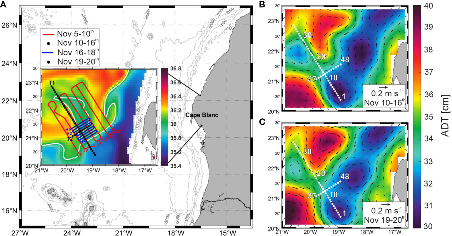
Figure 1 Map (A) of FLUXES II cruise presenting the low-resolution (red line) and high-resolution (blue line) SeaSoar grids and the two biogeochemical transects, T1 and T2 (black dots) over a salinity plot representing an average of all cruise days (Nov 5^th – 20^th) at 155.85 m depth. Made with GLORYS reanalysis. The white line represents the Cape Verde Front at a salinity of 36.045. Average Absolute Dynamic Topography with derived geostrophic field superimposed at the time of (B) T1 and (C) T2.

Organic matter (OM) either produced in situ or transported from elsewhere contributes differently to the BCP depending on whether it is dissolved (DOM), suspended (POM) or sinking (Sanders et al., 2014; Boyd et al., 2019). DOM is the largest pool of OM in the oceans; it is made up of myriads of compounds of marine and terrestrial origin, participating in a wide variety of production, transformation and removal processes (Hansell, 2013; Repeta, 2015). Although most of the DOM pool is refractory, either of autochthonous or allochthonous origin, a small fraction is photo-reactive and/or bioavailable (Hansell, 2013) and contributes to the BCP through the recycling and export of marine primary production. The optical properties of DOM allow to go a step further in the chemical and structural characterization of the colored and fluorescent fractions of DOM and its role in the BCP (Stedmon and Nelson, 2015; Nelson and Gauglitz, 2016). Colored dissolved organic matter (CDOM) is the fraction of DOM that absorbs light in the UV and visible spectrum (del Vecchio and Blough, 2002). The most commonly used absorption coefficients for tracing the different CDOM fractions are positioned at 254 nm (a_CDOM(254)) and 325 nm (a_CDOM(325)), which are proxies to the concentration of conjugated carbon double bonds (Weishaar et al., 2003) and aromatic rings (Nelson et al., 2004), respectively. The absorption spectral slopes between 275 and 295 nm (S_275-295) and between 350 and 400 nm (S_350-400) and its ratio S_R are commonly used to trace the origin, photochemical transformations, and average molecular weight of DOM (Helms et al., 2008). A small fraction of CDOM can re-emit light at a longer wavelength and it is called fluorescent DOM (FDOM). FDOM is divided into two main groups of fluorophores with contrasting excitation/emission wavelengths: i) protein-like compounds absorbing at<300 nm and emitting at<400 nm which are associated mainly to the aromatic amino-acids, either free or into proteins, and therefore considered as a proxy of labile DOM, and ii) humic-like substances absorbing at >300 nm and emitting at >400 nm linked to terrestrial and marine humic and fulvic acids, which are considered as proxies of refractory DOM and tracers of the microbial degradation of OM (Coble, 1996; Stedmon and Nelson, 2015).

Similarly to DOM, the vertical profiles of suspended organic carbon (POC) and the C:N molar ratio of POM are used to trace the role of POM in the BCP (Nowicki et al., 2022). POC accumulates in the surface mixed layer, where it is produced, and then is transported downwards by advection and turbulent diffusion processes (Lévy et al., 2012; Nagai et al., 2015). Its concentration decreases dramatically through the epi- and mesopelagic layers, where it is consumed. Preferential consumption of N over C compounds leads to an increase of the C:N molar ratio with depth (Álvarez-Salgado et al., 2014). Conversely, the fate of sinking POM is mainly dictated by the settling velocity of the aggregates of marine snow, which can sink at tenths to hundreds of meters per day (Nowald et al., 2009; Riley et al., 2012).

The aim of this work is to disentangle the variability of DOM and POM in the CVFZ at the meso- and submesoscale range in relation to the physical and biogeochemical processes operating in the area during fall, the time of the year of most intense upwelling activity. First, we focus on the epipelagic layer (< 200 m depth), where the dominant physical processes are associated to the high-resolution variability created by meso- and submesoscale (meanders, eddies) structures at the front. Second, we study the mesopelagic layer (200 - 1500 m), where the dominant physical process is the mixing of water masses of contrasting origin. For the epipelagic layer we aim to test the impact of meso- and submesoscale structures on the biogeochemistry of the front, with particular emphasis on POM, DOM and its colored and fluorescent fractions, which present an anomalous band of elevated humic-like fluorescence below the pycnocline. For the mesopelagic layer we aim to assess whether the high mesoscale activity in the epipelagic layer has an imprint in the mesopelagic layer, the relevance of local vs. basin scale mineralization processes on the OM distributions, and the contribution of DOM and POM to the local apparent oxygen utilization at the front.

Materials and methods

Sampling strategy and analytical procedures

Data used in this study were collected during the FLUXES II cruise (2-24 November 2017, on board R/V Sarmiento de Gamboa), in the Cape Verde Frontal Zone (CVFZ, NW Africa). The cruise consisted on two main activities: 1) three SeaSoar grids for high-resolution characterization of the CVFZ; and 2) two biogeochemical transects at high spatial resolution (5 nautical miles, NM; 9.3 km). The SeaSoar (MKII, Chelsea Instruments) was equipped with conductivity-temperature-depth (CTD, SBE 911 plus), oxygen (SBE 43), fluorescence (SeaPoint SCF) and turbidity (SeaPoint STM) sensors. All the measures were carried out with a constant cruising speed of 8 knots, covering the depth range of 0-450 m. The first SeaSoar grid consisted of 7 transects covering a box of 120 x 90 NM (222.2 x 166.7 km) for a general characterization of the study area and the second grid consisted of 8 transects that covered a box of 45 x 35 NM (83.3 x 64.8 km) (Figure 1A). The third and last grid will not be considered in this manuscript. Current velocities were measured with a 75 kHz RDI ship Acoustic Doppler Current Profiler (sADCP) configured in narrow band (long range). The sADCP provided along track raw data every 5 minutes from 36 to 800 m depth. The three SeaSoar grids is a focus of a dedicated chapter by Burgoa (2022). Here, they will be used just to contextualize the two high-resolution (5 NM) biogeochemical transects performed after the first and second SeaSoar grids.

Sampling during the high resolution transects was carried out using a rosette sampler equipped with conductivity-temperature-depth (SBE911 plus), oxygen (SBE43), fluorescence of chlorophyll (SeaPoint SCF), turbidity (SeaPoint STM), transmittance (WetLabs C-Star) and nitrate (SUNA V2, SeaBird) sensors. The rosette included 24 Niskin bottles of 12 liters for water collection. A total of 48 hydrographic stations were sampled with 10 levels each from surface to 1500 m. The first transect consisted of a 175 NM (324 km) long section with 36 sampling stations and a horizontal resolution of 5 NM (9.3 km). The second transect, perpendicular to the first one, was 55 NM (102 km) long with 12 stations and the same horizontal resolution as in the first transect (Figure 1A).

Core variables

Conductivity, dissolved oxygen (O₂), fluorescence of chlorophyll (Chl-a) and nitrate sensors were calibrated with discrete water samples collected from the rosette. Salinity was calibrated using a Guildline 8410-A Portasal salinometer, and conductivity measurements were converted into practical salinity units using the (UNESCO, 1985) equation. A procedure adapted from Langdon (2010) was used to determine the dissolved oxygen (O₂) on board by the Winkler potentiometric method. The apparent oxygen utilization (AOU) was calculated following Benson and Krause (UNESCO, 1986), where AOU = O₂sat – O₂, with O₂sat being the oxygen saturation. Determination of Chl-a was made according to the method of Holm-Hansen et al. (1965). It consists of filtering 500 mL of water through a Whatman GF/F filter and, after that, pigments were extracted in acetone (90% v/v) stored at 4°C in the dark for 24h and then analyzed with a Turner Designs bench fluorometer model 10 AU, previously calibrated with pure Chl-a (Sigma Co.). Samples for inorganic nutrient determination were taken in 25 mL polyethylene vials directly from the Niskin bottle and kept frozen at -20°C until analyzed in the base laboratory. Nutrient concentrations were determined by segmented flow analysis in an Alliance Futura autoanalyser. Nitrate, nitrite, phosphate, and silicate were determined colorimetrically as described in Hansen and Koroleff (1999). Ammonium concentration was determined using the fluorometric method of Kérouel and Aminot (1997).

The pycnocline, which separates the surface mixed layer from the waters immediately below, has been defined as the depth of the maximum stability (squared Brunt-Väisälä frequency, N²max) (Doval et al., 2001). It was calculated as follows:

$\begin{array}{ll}{\text{N}}_{max}^2=g·\frac{\text{ln }({\rho }_z/{\rho }_{z-1})}{z-\left(z-1\right)}& (1)\end{array}$

where g is gravity acceleration (9.81 m s^–2), and ρ_z is density at atmospheric pressure at depth z (in kg m^-3), calculated from salinity and temperature using the equation of UNESCO (1985).

Organic matter variables

Suspended organic carbon (POC) and nitrogen (PON) were determined by collecting 5 L of water from the Niskin bottles and filtering through 25 mm Whatman GF/F pre-combusted filters (450 °C, 4h) using a vacuum system with a pressure difference<300 mm Hg. Filters were then placed into 2 mL Eppendorf vials and dried for 12h in a vacuum desiccator with silica gel. After that, filters were stored in a freezer at -20°C until analyzed in the base laboratory. Concentrations of POC and PON were determined by high temperature catalytic oxidation (900°C) in a Perkin Elmer 2400 elemental analyzer. The filters were not exposed to HCl fumes after checking their negligible CaCO₃ content.

For dissolved organic carbon (DOC) determination, 25 mL of water were collected into pre-combusted borosilicate glass vials and frozen at -20°C until their subsequent analysis in the laboratory, performed by high temperature catalytic oxidation (680°C) in a Shimadzu TOC-V (Pt-catalyst). Seawater was not filtered due to the low concentration of particulate matter. Samples were melted, acidified (pH< 2) and degassed with high purity N₂ before measurements. Potassium hydrogen phthalate (KHP; Merck) was used as standard to calibrate the equipment and consensus reference materials provided by Hansell’s CRM Program (University of Miami, USA) were used to check the instrument performance. Our concentrations for the deep-sea water reference (Batch 16 Lot # 05-16) were 44.9 ± 1.7 µmol L^-1 (n = 10) while the certified values are 43-45 µmol L^-1.

Regarding the measurement of the colored (CDOM) and fluorescent (FDOM) fractions of DOM, water samples were collected in 250 mL acid-cleaned glass flasks and filtered through a 47 mm Whatman GF/F pre-combusted filter (450°C, 4h) with an all-glass filtration system under a positive pressure of high purity N₂. Filtered seawater was stored in the dark allowing to warm up to room temperature until on board analysis in the respective measuring cuvettes of the spectrophotometer for CDOM and spectrofluorometer for FDOM. Absorption spectra of CDOM were recorded from 700 to 250 nm at 0.5 nm intervals with a spectrophotometer Jasco V-750 equipped with 100 mm path length quartz cells. Milli-Q water was used as a reference blank. The absorption coefficient spectra a_CDOM(λ) (m^-1) were corrected by subtracting the Milli-Q spectrum and applying the equation:

$\begin{array}{ll}{\text{a}}_{\text{CDOM}}\left(\text{λ}\right)\mathrm{=23.03\hspace{0.17em}}\left[\text{Abs}\left(\text{λ}\right)\text{\hspace{0.17em}–\hspace{0.17em}Abs}\left(\mathrm{600-700}\right)\right]& (2)\end{array}$

where Abs(λ) is the absorbance at wavelength λ, Abs(600-700) is the average absorbance between 600 and 700 nm, which corrects for scattering primarily caused by fine particulate material and micro-air bubbles, and the factor 23.03 converts to natural logarithm and also considers the 0.1 m cell path length. The absorption coefficient indices used in this work were a_CDOM(254), a_CDOM(325), the spectral slope of the wavelengths bands 275-295 (S_275-295) and, 350-400 (S_350-400), and finally the ratio of both spectral slopes S_R (Helms et al., 2008).

FDOM measurements of previously filtered water were carried out in a Perkin Elmer LS-55 spectrofluorometer, and specific excitation-emission (Ex/Em) wavelength pairs were selected as described by (Coble, 1996). These Ex/Em pairs were 250/435 nm (peak A, general humic-like substances), 340/440 nm (peak C, terrestrial humic-like substances), 320/410 nm (peak M, marine humic-like substances) and 280/350 nm (peak T, tryptophan-like substances). Milli-Q water blank was subtracted from the samples analyzed each day in order to correct the Raman scatter band produced by water molecules and to normalize the fluorescence pair measurements to Raman units (RU) (Murphy et al., 2010). To test for instrument variability during the cruise, a sealed Milli-Q cuvette (Perkin Elmer) was analyzed daily to check for the Raman region, and p-terphenyl and tetraphenyl butadiene blocks (Starna) to check for the protein and humic-like substances regions, respectively (Catalá et al., 2015b). We chose to measure at these specific fluorescence peaks rather collecting Ex/Em matrices (EEMs) because of the time constrains of the high-resolution sampling strategy followed during the occupation of the biogeochemical transects.

Optimum multiparameter mesopelagic water mass analysis

An optimum multiparameter water mass analysis (Poole and Tomczak, 1999) was used to determine the relative contribution of the different water types (WTs) in the water samples collected through the mesopelagic layer. A common formation area and unique hydrographic characteristics defines each WT, mainly potential temperature and salinity, but also other chemical properties as oxygen, silicate, phosphate or nitrate (Poole and Tomczak, 1999; Tomczak, 1999). In this study, we used potential temperature (θ), salinity (S), silicate (SiO₄H₄) and NO as water mass tracers. The chemical parameter NO is defined as: $\text{NO}={\text{O}}_2+{\text{R}}_N{\text{NO}}_3-$, with R_N = 9.3 mol O₂ mol ${\text{NO}}_3^{-1}$ (Anderson, 1995) being the stoichiometric coefficient of oxygen consumption to nitrate production. A total of 9 WTs have been identified down to 1500 m: Madeira Mode Water (MMW); Eastern North Atlantic Central Water (ENACW) of 15°C and 12°C; South Atlantic Central Water (SACW) of 18°C and 12°C; Subpolar Mode Water (SPMW); Antarctic Intermediate Water (AA); Mediterranean Water (MW) and Labrador Sea Water (LSW). The thermohaline and chemical characteristics of each WT were taken from the literature (Table 1; Valiente et al., 2022).

TABLE 1

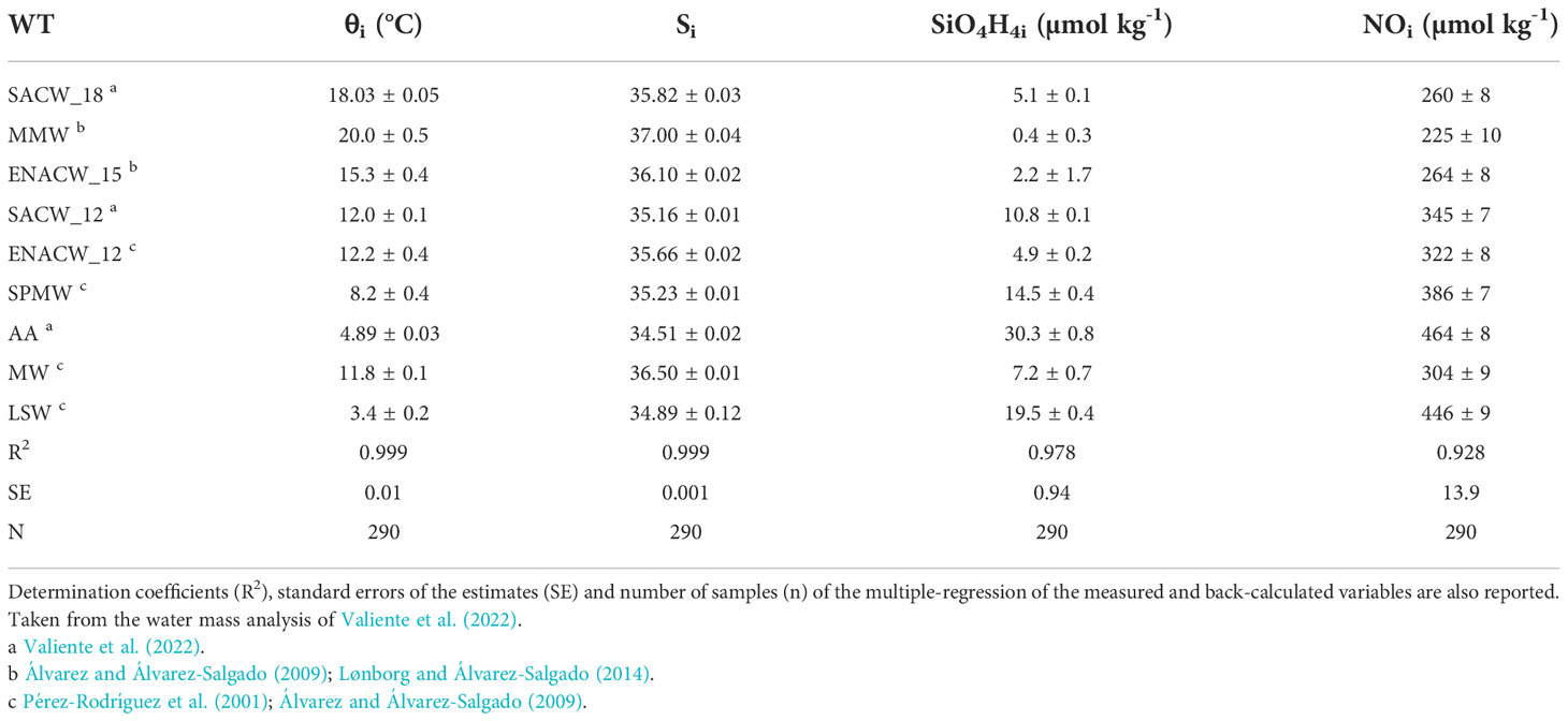
Table 1 Thermohaline and chemical characteristic (average value ± uncertainty) of the water types (WT) included in the Optimum Multi-Parameter Analysis (OMP) of the water masses present in the Cape Verde Frontal Zone (CVFZ).

To quantity the contribution of each WT to every sample, a set of 5 mass balance equations was solved using the values of θ, S, SiO₄H₄ and NO obtained for each sample collected during the cruise. The set of mass balance equations are:

$$\sum _i{X}_{ij}·{\theta }_i={\theta }_j+R{\theta }_j$$

$$\sum _i{X}_{ij}·S_i=S_j+R{S}_j$$

$$\sum _i{X}_{ij}· {(Si{O}_4{\text{H}}_4)}_i = {(Si{O}_4{\text{H}}_4)}_j+R{(Si{O}_4{\text{H}}_4)}_j$$

$$\sum _i{X}_{ij}·N{O}_i=N{O}_j+RN{O}_j$$

$\begin{array}{ll}\sum _i{X}_{ij}=1+R{\sum }^{}& (3)\end{array}$

where X_ij is the proportion of water type i in a sample j; θ_i, S_i, (SiO₄H₄)_i and NO_i are the values of θ, S, SiO₄H₄ and NO of WT i (Table 1); θ_j, S_j, (SiO₄H₄)_j and NO_j are the values of each variable in sample j; and R are the residuals of the mass balance equations and the mass conservation for sample j. These mass balance equations were normalized and weighted considering the measurement error of each parameter. Since we have 9 WTs and only 5 linear mixing equations, four mixing groups (see Supplementary Figure 1) were created based on expert knowledge of the hydrography of the study area (Valiente et al., 2022). Samples in the epipelagic layer were excluded from the OMP analysis due to the non-conservative behavior of θ, S, SiO₄H₄ and NO because of exchange of mass, heat and gases with the atmosphere and intense biological activity. Thus, a total of 290 out of 480 samples were included in the OMP analysis.

The WT proportion-weighted average value or archetype value of a variable N for each WT has been calculated from the concentration of N and the proportions of the 9 WTs identified in the study, using the following equation:

$\begin{array}{ll}{N}_i=\frac{{{\sum }^{}}_j{X}_{ij}·N_j}{{{\sum }^{}}_J{X}_{ij}}& (4)\end{array}$

where Ni is the archetype value of variable N in water type i, Xij is the proportion of WT i in sample j and N_j is the concentration of N in sample j. The standard error of the archetype value was obtained by:

$\begin{array}{ll}S{E}_{N_i}=\frac{\sqrt{{\sum }_j{X}_{ij}{\left(N_j-N_i\right)}^2}}{{\sum }_j{X}_{ij}}& (5)\end{array}$

Archetype values were determined for Z, S, θ, ${\text{NO}}_3^{-}$, AOU, DOC, TDN, POC, PON, CDOM indices and FDOM indices. Finally, the proportion of the total volume of the samples occupied during the FLUXES II cruise (%VOL_i) by a given WT i was calculated as:

$\begin{array}{ll}\%VO{L}_i=100·\frac{{\sum }_j{X}_{ij}}{n}& (6)\end{array}$

where n = 290, is the number of samples collected in the mesopelagic layer.

Multiple regression models

The fraction of the total variability of any non-conservative chemical variable N (DOC, POC, CDOM, FDOM) that is explained by water mass mixing in the mesopelagic layer can be calculated by applying a multiple linear regression of N_j with the water mass proportions X_ij (Perez et al., 1993). A system of n linear equations (one per sample) with 9 coefficients (one per WT) has to be solved for each chemical variable as follows:

$\begin{array}{ll}{N}_j=\sum _j{X}_{ij}·n_i+ R{N}_j& (7)\end{array}$

where n_i is the coefficient of WT i for parameter N and RNj is the residual of the equation for sample j. The determination coefficient (R²) of the multiple linear regression indicates the percent of explained variability and the standard error (SE) of the estimate defines the goodness of the fit.

Non-conservative variables depend not only on the mixing of water masses but also on the biogeochemical transformations that occur during that mixing. The variability associated to non-conservative processes is classified into (1) variability correlated with water mass proportions (basin-scale mineralization) and (2) variability independent of the water mass proportions (local-scale mineralization, in this case within the CVFZ). The first is modelled by the multiple linear regression of N_j with X_ij, (eq. 7). To account for the local-scale mineralization, the explanatory variable AOU is added to the linear regression model (eq. 8). A fitting parameter (coefficient β) is included to model the relationship between the chemical variables (e.g., DOC, POC, CDOM, FDOM) and AOU (Álvarez-Salgado et al., 2013; Álvarez-Salgado et al., 2014; Valiente et al., 2022):

$\begin{array}{ll}{N}_j=\sum _j{X}_{ij}·n_i+\beta ·AO{U}_j+R{N}_j& (8)\end{array}$

Remarkably, the coefficient β does not depend on WT mixing. In this sense, when calculating the multiple linear regression of DOC or POC with X_ij and AOU, the coefficient β indicates the contribution of DOC or POC to the local oxygen demand. Moreover, the contribution of DOC or POC to inorganic carbon production can be calculated by multiplying the coefficient β by the Redfield ratio of dissolved oxygen consumption to organic carbon mineralization of 1.4 mol O₂ mol C^-1 (Anderson, 1995).

Results

High-resolution mapping of the CVFZ in November 2017

When biogeochemical transect T1 was occupied (November 10^th to 16^th) satellite altimetry images revealed that most of the transect (stn 13 to 36) was edging the southwestern front of an anticyclonic eddy situated immediately to the northeast (Figure 1B). In contrast, the southern end of T1 (stn 1 to 13) was affected by a cyclonic eddy, whose core was at stn 4-5 (Figure 1B). During the occupation of the biogeochemical transect T2 (November 19^th to 20^th) the anticyclonic eddy displaced slightly to the northwest, changed its shape and intensified while the cyclonic eddy moved slightly to the south and weakened its intensity (Figure 1C).

A shallow intrusion of low salinity (S< 36.2) is clearly identified in the upper 40 m during the first SeaSoar grid (Figure 2A), which extended along the southern part of T1 and intruded through a body of higher salinity (S > 36.2). Between 40 - 200 m, the low salinity water body extended from the southeast to the northwest, occupying the southern half of T1. In addition, another water body with similar characteristics was located in the northern sector of the transect, leaving a narrow area of high salinity in between (Figure 2B). Biogeochemical transect T2 was occupied 3-4 days later than T1. Intense changes occurred in the salinity and current velocity plots, revealing that T2 was not synoptic with T1 at least in the upper 40 m, where the tongue of low salinity water (Figures 2A, B) disappeared, being occupied by a high salinity surface water body (Figure 2C). Below 40 m, the less saline water (S< 36.2) was displaced to the south being replaced by a higher salinity water body (S > 36.2) (Figure 2D). A detailed analysis of the high-resolution mesoscale activity during the cruise can be found in Burgoa (2022).

FIGURE 2

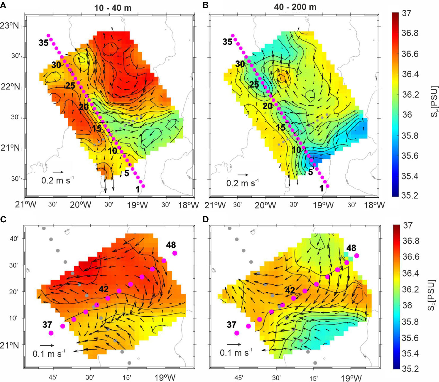
Figure 2 Average interpolated grids of salinity and horizontal velocity field superimposed between 10-40 m and 40-200 m at the time of (A, B) T1 and (C, D) T2. Current velocities were measured with the ship ADCP.

Supplementary Figure 2 shows the correspondence between transect L5 of the first SeaSoar grid and biogeochemical transect T1. L5 was occupied on November 8^th in 15.6 hours from northwest to southeast, while T1 transect took from November 10^th to 16^th from southeast to northwest. This means that the northwestern end of T1 was sampled 8 days after the SeaSoar grid while the southeastern end was sampled only 2 days after the SeaSoar grid. It is noticeable that the same mesoscale structures were observed during the occupations of L5 and T1, but larger differences were observed in the northern half of the transect consisting of a spatial displacement of the structures approximately 50 km to the north at the time of T1 occupation. On the contrary, the southern sector matched quite well due to a closer proximity in time.

Hydrographic variability of epipelagic waters along the biogeochemical transects

The Cape Verde thermohaline front (hereafter the Cape Verde Front, CVF) separates the warm and salty NACW from the cooler and fresher SACW. Zenk et al. (1991) defined the CVF as the intersection of the 150 m isobath with the 36 isohaline. Recently, Burgoa et al. (2021) extended its definition vertically and established an equation which define the front location at any depth from 100 to 650 m, based on an equal contribution (50%) of NACW and SACW. In the 100-200 m depth range the definition of Zenk et al. (1991) is very consistent with the Burgoa et al. (2021) and so we will use it to establish the hydrographic domains described below.

We identified a well-marked pycnocline along T1 and T2 (thick black line in Figure 3; see also Supplementay Figure 3A) ranging from 24 to 64 m (average, 42 m), which separates the warmer surface mixed layer from the colder sub-surface waters below. Three hydrographic domains were identified below the pycnocline along T1 according to the position of the CVF at 150 m. The depth of the 36 isohaline showed a marked variability, from 40 m at stn 6-8 to more than 200 m at stn 23-27. The CVF was crossed at stn 9 and 28 (dotted vertical lines in Figures 3–5 and Supplementay Figure 3). In domains A (stn 1-9) and C (stn 28-36) the low salinity SACW was the prevailing water mass, whereas domain B was mainly occupied by the high salinity NACW. Remarkably, a filament-shaped low-salinity intrusion was identified along domains A and B, consisting of a 25 m thick layer of water with S< 36 from 50 to 80 m. In domain A, the intrusion appeared connected with a SACW uplift, while in domain B, this lens of low salinity intruded into a body of higher salinity just below the pycnocline (Figure 3A, horizontal dotted line). In domain B and above this intrusion, a thin layer of higher salinity was observed coinciding with the position of the pycnocline, with maximum values at stns 13-15. Below the intrusion, there was a thicker high salinity water body down to 150 m with NACW characteristics coinciding with higher values of temperature (Supplementay Figure 3B) and lower values of AOU (Figure 3B) and ${\text{NO}}_3^{-}$ (Figure 3C).

FIGURE 3

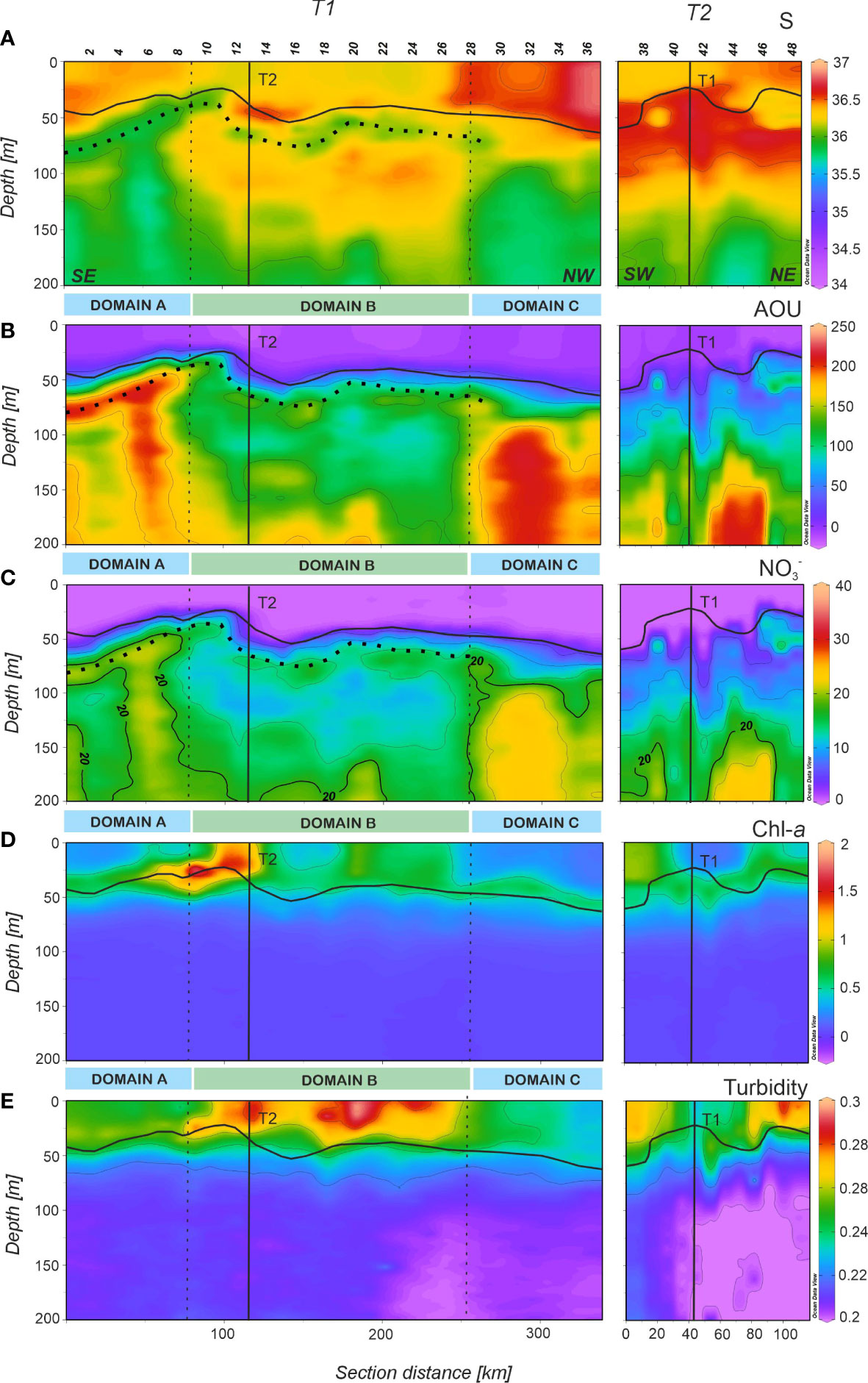
Figure 3 Distributions of (A) salinity (S), (B) apparent oxygen utilization (AOU) in µmol Kg^-1, (C) nitrate (${\text{NO}}_3^{-}$) in µmol Kg^-1, (D) chlorophyll-a (Chl-a) in µg L^-1 and (E) turbidity in NTU in the epipelagic layer of the FLUXES II cruise for the T1 (left) and T2 (right). All measurements were obtained at 1 db vertical resolution. T1 is divided into three domains (A-C) separated by vertical dotted lines at stn 9 and 28. Vertical black lines show the position of the orthogonal transects T2 and T1, respectively. Horizontal black line show the position of the pycnocline and horizontal black dotted line in a, b and c profiles show the position of the less saline intrusion (see text). Section distance is counting from southeast (SE) to northwest (NW) in T1 and from southwest (SW) to northeast (NE) in T2 (labelled at the bottom of the first panel). Produced with Ocean Data View (Schlitzer, 2017).

FIGURE 4

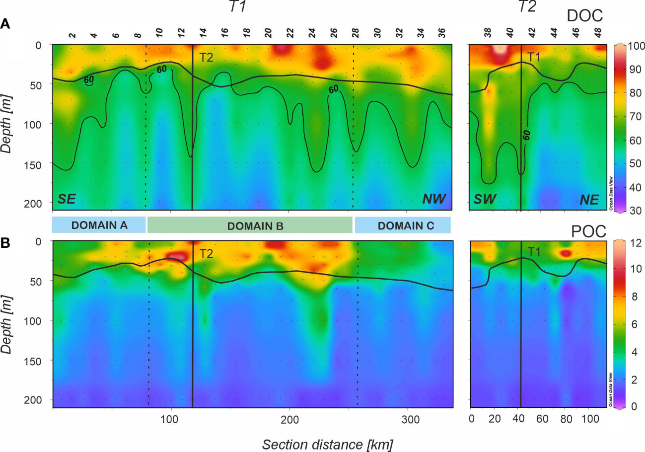
Figure 4 Distributions (A) dissolved organic carbon (DOC) in µmol Kg^-1 and (B) suspended particulate organic carbon (POC) in µmol Kg^-1 in the epipelagic layer of the FLUXES II cruise for the T1 (left) and T2 (right). T1 is divided into three domains (Domain A, Domain B and Domain C) separated by vertical dotted lines at stn 9 and 28. Dots represent samples and vertical black lines show the position of the orthogonal transect T2 and T1, respectively. Horizontal black line shows the position of the pycnocline. Section distance is counting from southeast (SE) to northwest (NW) in T1 and from southwest (SW) to northeast (NE) in T2 (labelled at the bottom of the first panel). Produced with Ocean Data View (Schlitzer, 2017).

FIGURE 5

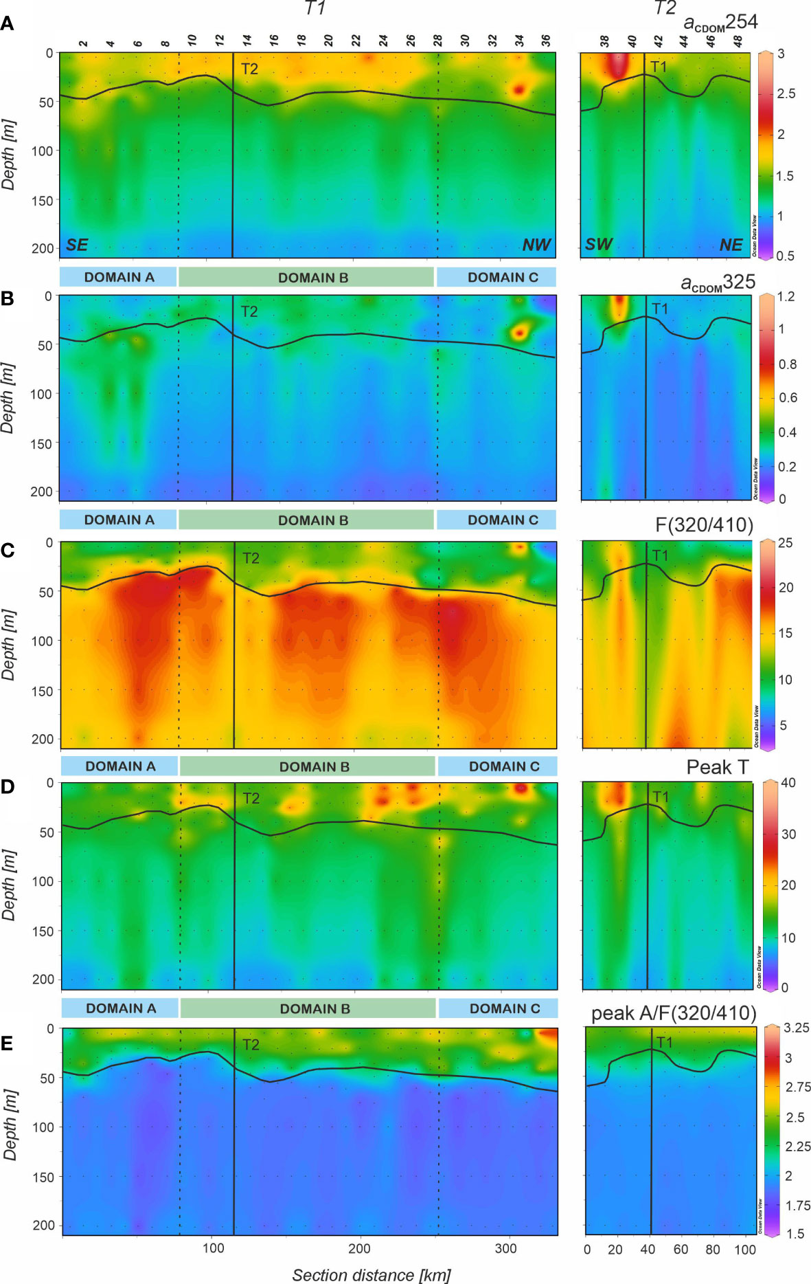
Figure 5 Distributions of (A) absorption coefficient at 254 nm (a_CDOM254) in m^-1, (B) absorption coefficient at 325 nm (a_CDOM325) in m^-1, (C) fluorescence at Ex/Em pair 320/410 nm (F(320/410)) in 10^-3 RU, (D) fluorescence at Ex/Em pair 280/350 nm (peak T) in 10^-3 RU, and (E) peak A to F(320/410) ratio (peak A/F(320/410)) in the epipelagic layer of the FLUXES II cruise for the T1 (left) and T2 (right). T1 is divided into three domains (A-C) separated by vertical dotted lines at stn 9 and 28. Dots represent samples and vertical black lines show the position of the orthogonal transect T2 and T1, respectively. Horizontal black line shows the position of the pycnocline. Section distance is counting from southeast (SE) to northwest (NW) in T1 and from southwest (SW) to northeast (NE) in T2 (labelled at the bottom of the first panel). Produced with Ocean Data View (Schlitzer, 2017).

In domain C, an intrusion of high salinity water (S > 36.5) in the surface mixed layer (Figure 3A) coincided with the highest values (p< 0.0005) of θ, 23.30 ± 0.04 °C (Supplementay Figure 3B; Table 2) and the lowest values (p< 0.0005) of Chl-a, 0.37 ± 0.01 µg L^-1 (Figure 3D; Table 2). Below the pycnocline down to 200 m, temperatures were significantly different between the three domains, with the highest values found in domain B (p< 0.0005; Table 2), occupied by NACW.

TABLE 2

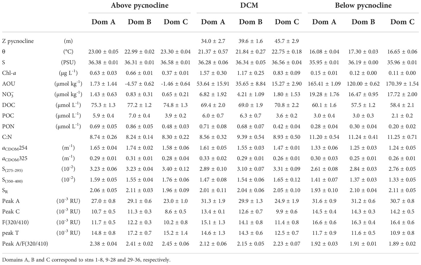
Table 2 Thermohaline and chemical characteristics (average value ± SE) of the epipelagic waters above and below the pycnocline and at the deep chlorophyll maximum (DCM) along the biogeochemical transect T1.

AOU was higher at the surface mixed layer in domain A (1.73 ± 1.44 µmol kg^-1) and domain C (-1.46 ± 0.64 µmol kg^-1) (Table 2), which contrasts with the significantly lower (p< 0.0005) values found in domain B (-4.57 ± 0.62 µmol kg^-1), suggesting higher net primary production in this sector. Below the pycnocline, average values of AOU were quite similar in domains A and C and again significantly lower (p< 0.0005) in domain B (Table 2), coinciding with the warmer and saltier water body of NACW (Figure 3B). The shallow and low salinity intrusion in this domain was also traceable in the AOU profile with slightly higher levels at 50-80 m. ${\text{NO}}_3^{-}$ distributions measured by a SUNA probe were well correlated with salinity (R² = 0.72, n = 9417) and especially with AOU (R² = 0.96, n = 9417). In domain A, the 20 µmol kg^-1 nitrate isoline uplifted from 90 m at stn 1 to 50 m at stn 8 (Figure 3C). Then, the isoline deepened abruptly to 165 m, coinciding with the CVF. In domain B, the 20 µmol kg^-1 nitrate isoline remained below 165 m attributable to the body of nutrient-poor NACW located above this depth. Finally, at stn 28, the isoline raised abruptly up to 100 m coinciding again with the CVF and the dominance of the nutrient-richer SACW in domain C. The shallow and low salinity intrusion present in domain B was also perceptible in the high ${\text{NO}}_3^{-}$ concentrations observed just below the pycnocline. Below the pycnocline, average values of ${\text{NO}}_3^{-}$ were significantly different between the three domains, with the lowest values found in domain B (p< 0.0005).

The DCM roughly coincided with the position of the pycnocline (Figure 3D), being at 33.8 m in domain A and at 45.5 m in domain C, while in domain B high chlorophyll reached the surface layer. Maximum values of Chl-a >1.5 µg L^-1 were found at stn 8-13, at the boundary between domains A and B. It is also noticeable that at stn 8-15, 18-26, 37-39 and 45-47, Chl-a was distributed homogeneously through the surface mixed layer instead of concentrating at the DCM. Turbidity (Figure 3E) shows the highest particle concentrations in the surface mixed layer and, particularly in domain B. In this domain, turbidity decreased northwestward, coinciding with lower values of Chl-a and higher values of temperature and salinity. Below the pycnocline, particle concentration decreased markedly, with significant differences between the three domains (p< 0.0005) and decreasing northwestward.

As explained in section 3.1, T2 was not synoptic with T1 and therefore failed to provide the desired 3D view of the CVFZ. Higher salinity water coming from the north displaced the low salinity water from the central sector of T1 at the time when T2 was occupied (Figure 2A, C). Salinity was also higher below the pycnocline, indicative again of this substitution of less salinity by higher salinity waters (Figure 3A). The SACW was located deeper at approximately 140 m, and the CVF was not observed along this transect. Chl-a distribution showed higher values at both ends of T2 and lower in the middle (Figure 3D). The distribution of turbidity was parallel to Chl-a with higher particle concentration at both ends of the transect (Figure 3E). Below the pycnocline, less turbidity was detected in the northeastern side of this section.

DOM, POM, CDOM and FDOM distributions in epipelagic waters along the biogeochemical transects

DOC presented an average concentration of 76.0 ± 0.8 µmol L^-1 along T1 in the surface mixed layer, with a maximum value of 97 µmol L^-1 located at stn 21 (Figure 4A), coinciding with the highest values of Chl-a and turbidity (Figure 3D, E). DOC decreased significantly with depth, but the distribution was not homogenous: columns of relatively high DOC values extending down to 200 m were surrounded by areas of lower concentration. DOC showed a significant correlation with AOU in epipelagic waters below the pycnocline (orthogonal distance regression (ODR); DOC = -0.15 (± 0.01)·AOU + 75.5 (± 1.3); R² = 0.49; n = 116). We excluded from this correlation surface mixed layer waters because of the impact of gas exchange with the atmosphere. According to the slope of this regression, DOC supports 21% of the oxygen demand in the epipelagic waters, assuming a Redfieldian -O₂/C stoichiometric ratio of 1.4 mol O₂ mol C^-1 (Anderson, 1995). Considering the three domains separately, domain B presented a significantly more negative slope (-0.18 ± 0.02) than domains A and C (-0.13 ± 0.04 and -0.15 ± 0.03, respectively). Therefore, while DOC supports 25.3% of the oxygen demand in domain B, this value decreases to only 18.5% and 21.0% in domains A and C, respectively.

The highest POC concentrations were observed at the surface mixed layer in domain B with an average value of 7.02 ± 0.35 µmol L^-1 (Figure 4B; Table 2). On the contrary, the lowest surface POC concentrations were found in domain C (3.88 ± 0.17 µmol L^-1). An average value of 2.78 ± 0.21 µmol L^-1 was obtained below the pycnocline all along T1, decreasing significantly (p< 0.05) from domain A to domain C (Table 2). POC correlated significantly with Chl-a (ODR; POC = 4.0 (± 0.2)·Chl-a + 1.7 (± 0.2); R² = 0.54; n = 235) and with DOC (ODR; POC = 0.21 (± 0.02)·DOC – 9.8 (± 0.7); R² = 0.44; n = 235) through the epipelagic layer. PON resembled the distribution of POC (ODR; POC = 7.4 (± 0.1)·PON + 0.6 (± 0.1); R² = 0.92; n = 235; data not shown). The C:N molar ratio of POM increased significantly with depth (p< 0005), from values > 8 in the surface mixed layer to values > 11 below the pycnocline for the three domains (Table 2). We also examined the correlation of the sum of DOC and POC with AOU (ODR; (DOC + POC) = -0.17 (± 0.02)·AOU + 80.32 (± 1.40); R² = 0.50; n = 116). The slope of the linear regression indicates that the dissolved and suspended particulate OM fractions support together 23.6% of the oxygen demand in the epipelagic waters below the pycnocline, the remaining being therefore supported by the sinking OM fraction. Again, domain B presented a significantly more negative slope (-0.21 ± 0.03) for the DOC+POC vs AOU correlation than domains A (-0.15 ± 0.04) and C (-0.16 ± 0.03). Therefore, DOC+POC supports 29.5% of the oxygen demand of epipelagic waters below the pycnocline of domain B, while only 20.4% and 22.6% in domains A and C, respectively.

The distribution of a_CDOM(254) (Figure 5A), a proxy to the abundance of conjugated carbon double bonds in DOM (Lønborg and Álvarez-Salgado, 2014; Catalá et al., 2018) was characterized by higher levels in the surface mixed layer that decreased gradually with depth (Table 2). The correlation of a_CDOM(254) with DOC was significant (ODR; DOC = 38.0 (± 1.7)·a_CDOM(254) + 11.4 (± 2.1); R² = 0.67; n = 240). Regarding a_CDOM(325) (Figure 5B), a proxy to the aromatic fraction of DOC (Nelson et al., 2004), the highest values were found again in the surface mixed layer with 0.30 ± 0.01 m^-1. Below the pycnocline the average value was significantly lower (p< 0.005) at 0.26 ± 0.01 m^-1. S_275-295, a proxy for the average molecular weight, origin and photochemical transformations of DOM, showed higher values in the surface mixed layer, with an average of 3.26 ± 0.04 10^-2 nm^–1 for T1. (Table 3) The average value decreased below the pycnocline (2.76 ± 0.03 10^-2 nm^–1), with the maximum value found in domain B (Table 3). Regarding the ratio S_R, average values were characteristic of ocean waters, similar above and below the pycnocline (2.08 ± 0.03 and 2.07 ± 0.04, respectively for T1) and no significant differences were found among the three domains.

TABLE 3

Table 3 Themohaline and chemical characteristics (arquetype value ± SE) of mesopelagic waters.

Fluorescence intensities of Coble’s (1996) humic-like peaks M and C showed a strong positive linear correlation (R² = 0.93). Therefore, both fluorophores display the same distribution in the study area. Overlapping of their respective fluorescence intensities is the anticipated reason behind this particular behavior. Consequently, we decided to use the fluorescence intensity of peak M as a measure of the concentration of humic-like substances in general, either marine or terrestrial. To avoid any confusion, we will use the term F(320/410) hereinafter. In general, the intensities of F(320/410) (Figure 5C) are lower in the surface mixed layer (Table 2). Remarkably, immediately below the pycnocline (between 50 and 150 m), F(320/410) presented a band of relatively high fluorescence with a maximum value of 24 x 10^-3 RU. Below this band, values decreased to about 15 x 10^-3 RU at 200 m. Analyzing the relationship between F(320/410) and AOU, three groups of samples can be identified (Supplementary Figure 4). Group 1 (green) represents the surface mixed layer (above the pycnocline) with low AOU; Group 2 (light blue) show the usual trend of humic-like substances accumulation with increasing AOU below the pycnocline; and Group 3 (navy blue) the anomalously high fluorescence of humic-like substances below the pycnocline. Coble’s (1996) peak A also shows a good correlation with F(320/410) (R² = 0.77) but the differences in the distribution of both fluorophores occur specifically in the surface mixed layer, where the ratio peak A/F(320/410) reaches particularly high values (Figure 5E). Significant differences between the three domains were not found, but there the ratio peak A/F(320/410) was significantly higher (p< 0.001) above than below the pycnocline (Table 2).

The protein-like fluorophore (peak T; Figure 5D) showed higher intensities in the upper 30 m and decreased abruptly with depth. For the surface mixed layer, peak T in domain A was significantly lower (p< 0.025) than in domain B, and at the DCM, domain C was characterized by significantly lower peak T intensities than domain B (p< 0.05). Below the pycnocline, the distribution was not homogeneous and, analogously to DOC, columns of higher peak T intensities were found reaching down to 200 m.

When T2 was occupied, DOC showed the highest value at the surface of stn 39 with 116.7 µmol L^-1 and lower values were found in the eastern end of the transect. Below the pycnocline, higher DOC values were measured in the western end with a similar distribution in columns as in T1. POC resembled the distribution of turbidity with higher values at both ends of T2 and slightly lower at the middle of the section. CDOM and FDOM measurements were also similar to those in T1 except for a remarkably higher value above the pycnocline at stn 39 in all the profiles (Figure 5). F(320/410) showed similarly high intensity as in T1 below the pycnocline in the easternmost part of the transect, whereas at stns 40-42 the intensity was lower.

Hydrography of mesopelagic waters

The shallowest central water mass, SACW_18, was centered at 165 ± 25 m and represented 3.2% of the total sampled water volume (Table 3; Figure 6). MMW was centered at 201 ± 1 m but represented only 0.1% of the total volume, so it was almost negligible. ENACW_15 was below MMW, at an average depth of 232 ± 11 m and represented 12.3% of the total sampled volume. The last two central water masses were SACW_12 and ENACW_12, centered at 339 ± 24 and 453 ± 17 m (Table 3), and with a total sampled volume of 8.6 and 26.1%, respectively. Therefore, ENACW_12 was the most representative central water mass of the study area.

FIGURE 6

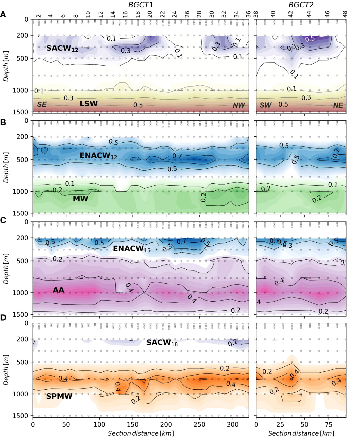
Figure 6 Distributions of the water masses present in the CVFZ during the FLUXES II cruise. Water mass proportions in this figure were derived from an OMP analysis applied to CTD data at 1 dbar vertical resolution. θ and S were measured directly with the CTD, while SiO₄H₄ and NO values were reconstructed by fitting the measured water sample concentrations to a non-linear combination of variables directly measured with the CTD (θ, S, O₂). The distribution of the water-masses among the panels was designed to avoid contour overlapping and does not follow an oceanographic criteria. (A) SACW_12 and LSW; (B) ENACW_12 and MW; (C) ENACW_15 and AA; and (D) SACW_18 and SPMW. Section distance is counting from southeast (SE) to northwest (NW) in T1 and from southwest (SW) to northeast (NE) in T2 (labelled at the bottom of the first panel).

The intermediate and upper deep waters were occupied by four water masses. SPMW and AA were placed at 813 ± 20 and 904 ± 36 m (Figure 6), and represented 10.4 and 20.2% of the total sampled water volume, respectively (Table 3). These water masses were followed by MW and LSW, centered at 1225 ± 62 and 1443 ± 26 m, and representing 5.6 and 13.4% of the total sampled water volume, respectively.

AOU in the central waters showed lower values in the central part of T1 between stn 8 and 28 that corresponded with a higher contribution of ENACW (Figure 7A). Maximum AOU levels were observed in SACW_12, with an archetype concentration of 191.0 ± 4.2 µmol kg^-1, followed by ENACW_12 and SPMW with 186 and 187 µmol kg^-1, respectively (Table 3). The lowest value in the central waters was 112 µmol kg^-1 for MMW, and in the deep waters, the archetype AOU concentration was 128 µmol kg^-1 for LSW.

FIGURE 7

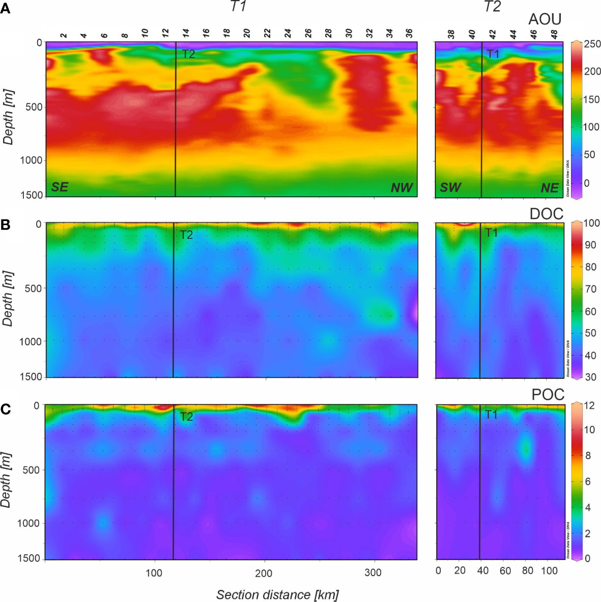
Figure 7 Distributions of (A) apparent oxygen utilization (AOU) in µmol Kg^-1, (B) dissolved organic carbon (DOC) in µmol Kg^-1, and (C) suspended particulate organic carbon (POC) in µmol Kg^-1 in the 0-1500 m depth range of the FLUXES II cruise for the T1 (left) and T2 (right). Dots represent samples (AOU measurements were obtained at 1 dbar vertical resolution) and vertical black lines show the position of the orthogonal transect T2 and T1, respectively. Note that the y-axis (depth) is not linear. Section distance is counting from southeast (SE) to northwest (NW) in T1 and from southwest (SW) to northeast (NE) in T2 (labelled at the bottom of the first panel). Produced with Ocean Data View (Schlitzer, 2017).

DOM, POM, CDOM and FDOM distributions in the mesopelagic waters

DOC showed a gradual decrease with depth starting with an archetype value of 52.8 ± 1.9 µmol L^-1 in SACW_18 and ending with 41.8 ± 0.7 µmol L^-1 in LSW (Figure 7B). Water mass mixing (eq. 7) explained 40% of the DOC variability in the CVFZ with an SE of 4.5 µmol L^-1 (Table 4). When adding AOU to the multiple linear regression model (eq. 8), the DOC - AOU coefficient was not significant. The distribution of POC (Figure 7C) was similar to DOC, with a general decrease of concentration with depth. The mixing model (eq. 7) explained 38% of POC variability with a SE of 0.4 µmol L^-1 and as for the case of DOC, when including AOU in the regression model (eq. 8), the POC - AOU coefficient was not significant. Regarding of PON, the distribution was similar to POC with a high correlation between both variables (ODR; POC = 11.6 (± 0.4)·PON + 0.29 (± 0.03); R² = 0.76; n = 288). The multiple linear regression model explained 54% of the variability of PON in the CVFZ with a SE of 0.03 µmol L^-1 and again no significant PON - AOU coefficient was found when adding AOU to the multiple regression model. The C:N ratio of POM increased significantly with depth, from an archetype value of 12.23 ± 0.90 in SACW_18 to a value of 19.48 ± 0.68 in LSW (Table 3). It is noticeable that the ratio was the highest in the northern part of T1 from stn 24 to 36 and in the depth range of 750-1500 m with a maximum local value of 27.49 in stn 32 at 1500 m.

TABLE 4

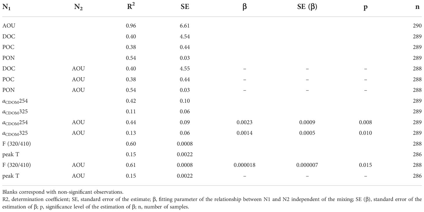
Table 4 Parameters of the linear mixing (Eq. 7) and mixing-biogeochemical (Eq. 8) models.

Regarding the distribution of CDOM, archetype values of a_CDOM(254) were the highest in SACW_18 and then decreased with depth to the lowest value found in MW (Table 3; Figure 8A). The mixing model explained 42% of the a_CDOM(254) variability in the dark ocean and increased to 44% when AOU is added to the linear regression. In this case, the a_CDOM(254) - AOU coefficient was significant (0.0023 ± 0.0009 m^–1 kg µmol^–1; Table 4). Archetype a_CDOM(325) values of the different water masses ranged between 0.16 m^-1 in MMW and MW, and 0.22 m^-1 in SACW_18 (Figure 8B). The WTs mixing model explained only 11% of the a_CDOM(325) variability, increasing to 13% when adding the AOU variable to the model and the a_CDOM(325) - AOU coefficient was also significant (0.0014 ± 0.0005 m^–1 kg µmol^–1; Table 4). In the central waters, the highest value of the spectral slope S_275-295 was found in MMW and then decreased with depth and remained stable in the intermediate and deep waters. Concerning the ratio S_R, in the central water masses the highest value corresponded to the MMW and then decreased in LSW (Table 3).

FIGURE 8

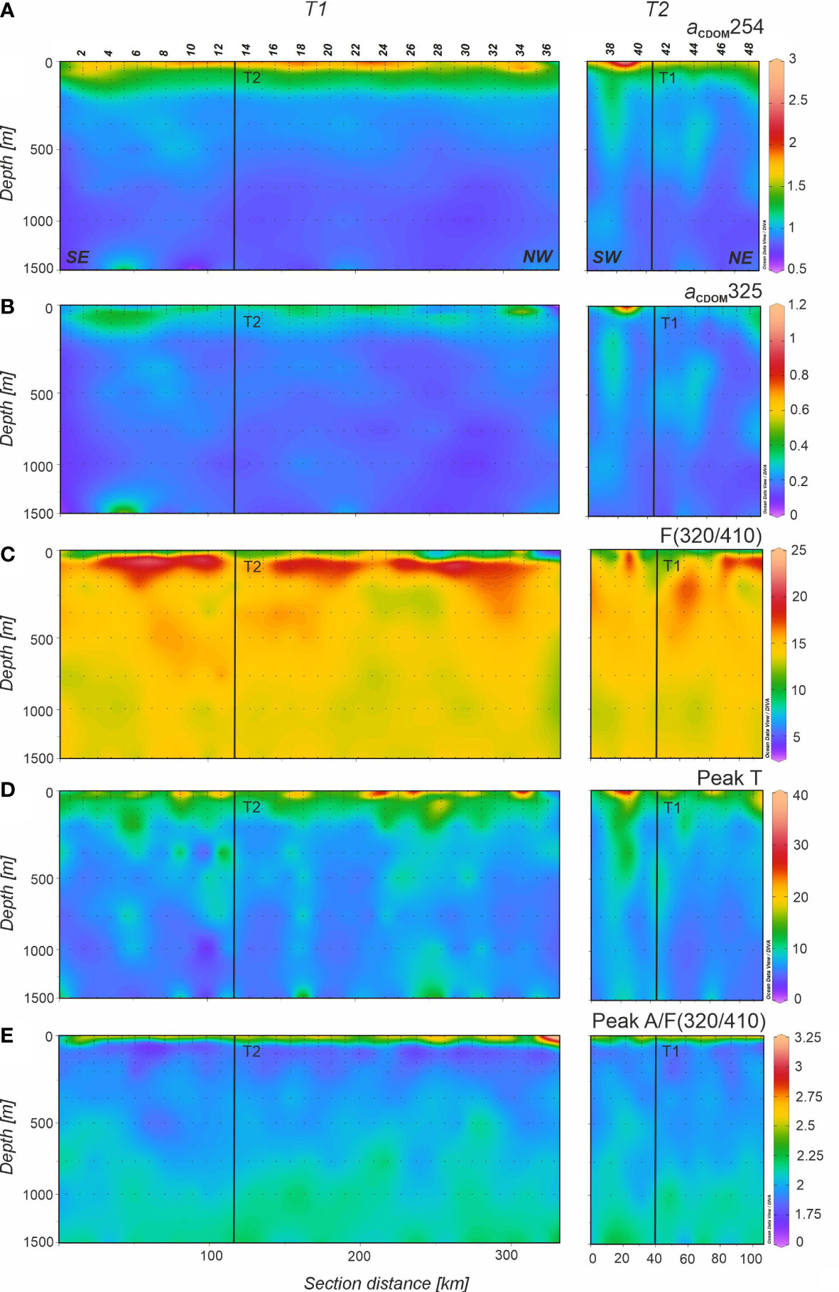
Figure 8 Distributions of (A) absorption coefficient at 254 nm (a_CDOM254) in m^-1, (B) absorption coefficient at 325 nm (a_CDOM325) in m^-1, (C) fluorescence at Ex/Em pair 320/410 nm (F(320/410)) in 10^-3 RU, (D) fluorescence at Ex/Em pair 280/350 nm (peak T) in 10^-3 RU, and (E) peak A to F(320/410) ratio (peak A/F(320/410)) in the 0-1500 m depth range of the FLUXES II cruise for the T1 (left) and T2 (right). Dots represent samples and vertical black lines show the position of the orthogonal transect T2 and T1, respectively. Note that the y-axis (depth) is not linear. Section distance is counting from southeast (SE) to northwest (NW) in T1 and from southwest (SW) to northeast (NE) in T2 (labelled at the bottom of the first panel). Produced with Ocean Data View (Schlitzer, 2017).

With regard to FDOM, the maximum intensity of F(320/410) in the central waters was recorded in SACW_18 associated with the subsurface maxima situated just below the high fluorescence intensity band all along T1 (Figure 8C). F(320/410) intensity decreased from SACW_12 to LSW, although it remained quite constant in intermediate waters. The distribution of peak A to F(320/410) (Figure 8E) indicates that differences occur mainly in the surface mixed layer. Protein-like fluorescence intensities gradually decreased with depth reaching the lowest levels at 800 m in SPMW and then increased again but very slightly. In Figure 8D it is noticeable the columns of high peak T intensity reaching 1500 m depth in T1 and T2 profiles. The mixing model explained 60% of the total variability of F(320/410) in mesopelagic waters with a SE of 8 10^-4 RU. On the contrary, only 15% of peak T variability was explained by the mixing model with a SE of 2.2 10^-3 RU. When AOU is added to the multiple linear regression, the explained variability of F(320/410) increased to 61% with a significant F(320/410) - AOU coefficient (1.8 ± 0.7 10^–5 RU kg µmol^–1) whereas inclusion of AOU in the multiple regression of peak T does not produce a significant peak T – AOU coefficient (Table 4).

Discussion

Physical-biogeochemical coupling in the CVFZ

The main hydrographic structures found in the area are the thermohaline front (CVF) and the intrusion of low salinity (S< 36) located below the pycnocline along T1. This nutrient-rich lens about 20-30 m thick extended along the first 135 NM (250 km) of T1 and provided nutrients to the immediately above surface waters, contributing to the high values of Chl-a along these domains (Figures 3C, D). Hosegood et al. (2017) also brought up the importance of mesoscale processes in injecting nutrients to the euphotic zone and stimulating higher levels of primary production. Moreover, the southern sector of T1 was affected by a cyclonic eddy (Figures 1B, C) transporting SACW that is responsible for the uplift of the pycnocline from stns 1 to 10, explaining also the connection with the low salinity intrusion observed in the southern section of T1. On the contrary, the middle and mostly the northern sector of T1 were affected by an anticyclonic eddy that deepened the pycnocline. Additionally, current velocities indicate that waters affected by the anticyclonic eddy were moving northward, distributing the Chl-a and turbidity in that direction, while currents in the southern part of the transect were less intense and directed southward (Figures 2A, B).

The average values of DOC in the epipelagic layer are very similar to that found in Valiente et al. (2022) in the same area during summer 2017. They reported similar DOC distribution patterns with columns of relatively high values interspersed with areas of low concentration. This phenomenon could be related with the intense meso- and submesoscale activity in this frontal zone, where mixing can favor the downward transport of DOC and POC (Lévy et al., 2012; Nagai et al., 2015) combined with the dissolution of fast sinking particles as previously suggested by Lopez et al. (2020). Moreover, fast sinking particles in this area are linked to Sahara dust inputs, which plays an important ballasting role and therefore transporting DOC adsorbed onto these particles down to the dark ocean. Numerous studies related the presence of lithogenic material originating from NW Africa with a higher efficiency of the biological carbon pump, increasing the particle density and settling rates (Iversen et al., 2010; Fischer et al., 2016; van der Jagt et al., 2018). Similar striped-like patterns were also observed for POC, especially at stn 24-25.

The linear correlation between DOC and AOU indicates that DOC supported about 21% of the oxygen demand of epipelagic waters. When considering both the dissolved and suspended organic carbon fraction, the value increased slightly to 23.6%, revealing that the sinking organic carbon fraction should be the main contributor to oxygen consumption and OM mineralization in the epipelagic layer. DOC contribution to the oxygen demand in epipelagic waters is similar to previously reported in other areas: e.g. 21% in the Red Sea (Calleja et al., 2019), 15-41% in the Sargasso Sea (Hansell and Carlson, 2001), 21-47% in the South Pacific and 18-43% in the Indian Ocean (Doval and Hansell, 2000), and 30% in the Eastern Subtropical North Pacific, north of the gyre (Abell et al., 2000). It is noticeable the significant differences in the DOC-AOU slope in mesopelagic waters between domains A, B and C. The higher contribution of DOC and suspended POC to the oxygen demand in domain B is likely due to larger production of fresh OM in this domain, therefore susceptible to faster degradation.

A significant linear relationship between DOC and a_CDOM(254) was found, which suggests that the latter could be used as an optical proxy of the former as was stated in previous works (Lønborg and Álvarez-Salgado, 2014; Catalá et al., 2018). The linear ODR of DOC and a_CDOM(254) for the whole sample set of epipelagic and mesopelagic waters (R² = 0.80, n = 478) yielded an origin intercept of 9.7 (± 1.0) µmol L^-1, similar to the values found by (Lønborg and Álvarez-Salgado, 2014) in the Eastern North Atlantic (10 µmol L^-1) and by Catalá et al. (2018) in the Mediterranean Sea (9 µmol L^-1). The slope of the regression, 39.1 (± 0.9) m² mmol^–1, was also close to those found in the two previous studies in the NE Atlantic, 40 ( ± 1) m² mmol^–1, and the Mediterranean Sea, 46 ( ± 1) m² mmol^–1. Exploring the relationship between a_CDOM(254) and DOC in different ocean areas is a subject of interest in order to decipher whether there is a universal relationship between both parameters or if it varies depending on the region.

Since a_CDOM(325) is a proxy for the concentration of aromatic dissolved organic compounds, it is expected to be sensitive to solar irradiation that produce photodegradation (Nelson et al., 2004; Catalá et al., 2015a). Nevertheless, in the CVFZ we found significantly higher a_CDOM(325) values above than below the pycnocline. Since the elevated values of S_275-295 and peak A/F(320/410) indicate active DOM photodegradation in the surface mixed layer, the high a_CDOM(325) levels there should be due to an in situ production and/or external supply exceeding photodegradation. In this regard, the existence of an external CDOM and FDOM source is hypothesized in the next section. Note that the high levels of the peak A/F(320/410) ratio in the surface mixed layer are due to the much higher sensitivity of F(320/410) than peak A to phtochemical degradation when irradiated with natural UV light (Martinez-Perez et al., 2019).

Humic-like fluorescence maximum in epipelagic waters

The CVFZ is, to the best of our knowledge, the first marine system where a layer of relatively high humic-like fluorescence intensity is found below the pycnocline, preferentially down to 150 m (Figures 5C), although this signal is also detectable in mesopelagic waters (Figure 8C). Its relationship with AOU (dark blue squares in Supplementary Figure 4) does not follow the expected linear trend, with a slope of 2.8 10^-5 RU·kg^–1·µmol, due to microbial respiration (light blue circles in Supplementary Figure 4). This slope is in accordance with the values reported in other studies covering the world ocean: 2.5 10^-5 RU·kg^–1·µmol in Catalá et al. (2015a) and 2.7 10^-5 RU·kg^–1·µmol in Jørgensen et al. (2011). We hypothesize that the input of Sahara dust could be the reason behind this band of relatively high humic-like fluorescence intensity compared to their surroundings. To test this hypothesis, we ran an experiment consisting on adding Sahara dust (collected in a quartz fiber filter) to seawater to obtain the seawater-soluble fraction (SSF) and analyzed the changes of the DOM characteristics (see material and methods in the Supplementary Information). The results of this comparison is shown in Supplementary Table 1: while the DOC supplemented by 25.50 mg of Sahara dust in 100 mL of seawater (67.6 ± 1.3 µmol L^-1) is comparable to the concentration found in the epipelagic waters below the pycnocline (57 - 77 µmol L^-1; Table 2), F(320/410) values are 6 - 10 times higher in the Sahara dust, which suggest that Sahara dust contains highly reworked DOM with a large proportion of humic-like compounds. a_CDOM(325) is >4 times higher than in situ and significant changes are also observed in S_(275-295) and S_R (Table 2 and Table S1). In particular, S_R values for the CDOM transported by Sahara dust was 0.9, i.e. lower than 1, which is distinctive of DOM with continental origin (Helms et al., 2008).

Local mineralization in the water masses of the mesopelagic layer of the CVFZ

The distribution of DOC, POC and PON in mesopelagic waters showed the expected decrease with depth due to production in the surface layer and subsequent mineralization at depth. POC concentration was very low compared to other studies in the Canary Current System (Alonso-González et al., 2009; Arístegui et al., 2020). As shown in Valiente et al. (2022), these differences could be due to the influence of the giant filament of Cape Blanc, which exports the suspended POC fraction further offshore whereas the sinking POC fraction is mineralized in the epipelagic and upper mesopelagic waters. The C:N molar ratios of POM reported in this work for both the epi- and mesopelagic layers are higher than the canonical Redfield ratio of 6.6 (Redfield et al., 1963; Anderson, 1995) and also higher than values reported in other works (see compilation by Schneider et al., 2003). The ratio increases from 8 at the surface, 11 at the base of epipelagic layer (200 m), to 19.5 at the base of the mesopelagic layer (1500 m). Similar values were found in Valiente et al. (2022) for a wider sampling area in the CVFZ and in a different season. This increase of the C:N molar ratio of suspended OM with depth indicates a preferential degradation of N compounds at shallower depths, and therefore, increased the relative abundance of C over N with depth (e.g., Álvarez-Salgado et al., 2014).

The water mass mixing model (eq. 7) explained 40%, 38% and 54% of the variability of DOC, POC and PON, respectively, and no significant increase of the variability explained by the model occurs when adding AOU as explanatory variable. These results indicate that the imprint of mineralization observed in mesopelagic waters of the CVFZ does not occur locally but during the pathway of the water masses from their respective formation sites to the CVFZ. The low contribution of DOC and POC to local mineralization also suggests sinking POC should be the primary support for the local oxygen demand. Nevertheless, other works further north in the Canary Current system (Arístegui et al., 2003; Arístegui et al., 2020), where the concentration of suspended POC is much higher, found that this fraction was the main support for mesopelagic respiration there. These authors argued that advection of this suspended particulate material from the adjacent coastal productive waters is the reason behind this behavior.

Mixing and mineralization are the main processes controlling DOM and POM variability in mesopelagic waters, but other processes like absorption-desorption of DOM onto particles exist and can be relevant as abiotic removal of DOM from the upper layers (Druffel and Williams, 1990). This mechanism is related with the well-known ballasting effect of the lithogenic material (both biominerals and atmospheric inputs) (Bory and Newton, 2000; Fischer and Karakaş, 2009; Fischer et al., 2016; van der Jagt et al., 2018) and could explain the columns of high DOC concentration through the epipelagic layer observed in the CVFZ, where the flux of sinking particles is substantial.

Contrary to what has been observed for DOC, POC and PON, the mixing models for a_CDOM(254) and a_CDOM(325) improved significantly when AOU was included (Table 4) indicating that local mineralization processes at the CVFZ contributed to explain the variability of the colored but not the bulk fraction of DOM. Moreover, the regression coefficients of a_CDOM(254) and a_CDOM(325) with AOU were positive, indicating the generation of colored organic compounds with increasing AOU. Given that we have not observed significant local DOC mineralization, the accumulation of a_CDOM(254) and a_CDOM(325) should be related to the predominant mineralization of the sinking fraction of POC as already suggested in a previous work (Valiente et al., 2022). Therefore, part of a_CDOM(254) and a_CDOM(325) would represent refractory by-products of the mineralization of bioavailable sinking organic carbon, in agreement with the microbial carbon pump concept (Jiao et al., 2010; Catalá et al., 2015a; Legendre et al., 2015), which states that a fraction of the labile OM respired by marine organisms is converted to recalcitrant DOM. In other systems, as the Mediterranean Sea, where the contribution of sinking POC is less important, the coefficients of a_CDOM(254) and a_CDOM(325) with AOU are negative (Catalá et al., 2018), indicating a net consumption of this colored fraction rather than its production.

Regarding the fluorescent fraction of DOM, the mixing model explained 60% of the total variability of F(320/410), indicating that basin scale processes occurring from the WTs formation sites to the CVFZ were the main drivers of the variability. On the contrary, the explained variability of peak T was only 15%, revealing the lability of these protein-like compounds that are produced mainly in the upper layers of the ocean (Jørgensen et al., 2011). Inclusion of AOU improved significantly the mixing model for F(320/410), indicating that local mineralization processes contributed to the production of F(320/410) in the mesopelagic layer of the CVFZ, with an AOU coefficient of 1.8 (±0.7) 10^–5 RU µmol kg^–1 (Table 4). This value is very similar to that reported in Martínez-Pérez et al. (2019) for the Mediterranean Sea (2.1 ± 0.4 10^-5 RU µmol kg^–1), who applied the same mixing-AOU model. These coefficients, independent of water mass mixing, are somewhat lower than the slope of the direct linear F(320/410)-AOU correlation: 2.8 RU µmol kg^–1 (this work; Figure S4), 2.7 10^-5 RU µmol kg^–1 (Jørgensen et al., 2011) or 2.5 RU µmol kg^–1 (Catalá et al., 2015a). This indicates that direct correlations overestimate the conversion factors of labile into refractory DOM.

Conclusions

The distribution of DOM, POM and its colored and fluorescent fractions is dictated by meso- and submesoscale structures (eddies, meanders) that were captured at a high-resolution sampling (< 10 km) and showed a tight coupling between physical and biogeochemical parameters. A relatively high band of fluorescent humic-like DOM below the pycnocline is hypothesized to be released from sinking Sahara dust particles based on an anomalous relationship with apparent oxygen utilization. In the mesopelagic layer, the mineralization of DOM and POM occurs mainly during the transit of the water masses from their respective formation sites to the CVFZ since a low contribution is observed to the local oxygen demand. The local mineralization is dictated by fast-sinking POM (autochthonous or allochthonous) favored by the well-known ballasting effect of lithogenic material that have been studied previously in the NW African upwelling system. This local mineralization leads to an increment in the C:N ratio due to preferential nitrogen compounds consumption and also to the production of colored refractory DOM through the microbial carbon pump mechanism, as indicated by the positive relationship between a_CDOM(254), a_CDOM(325) and F(320/410) with AOU.

Data availability statement

The raw data supporting the conclusions of this article will be made available by the authors, without undue reservation.

Author contributions

RC, NB, BF-C, SV, NH-H, AR-S and AM-D participated in the FLUXES II oceanographic cruise and contributed with data acquisition. NB, FM, AM-D, AR-S, IH-G, AM-M processed the physical data. BF-C carried out the OMP analysis. RC, SV, XA-S, MN-C, MG-C, AM-P, AD-H, NH-H and JA contributed with biogeochemical data acquisition and processing. JA and XA-S conceived and designed the oceanographic cruise and gave the resources. RC analyzed and interpreted data and wrote the first draft of the manuscript. All authors contributed to the article and approved the submitted version.

Funding

This work was funded by Spanish National Science Plan research grants FERMIO (CTM2014–57334–JIN) and FLUXES (CTM2015-69392-C3), co–financed with FEDER funds, and e-IMPACT (PID2019-109084RB-C21 and –C22). RC, SV and NB were supported by predoctoral fellowships from the Spanish Ministry of Science and Innovation (BES-2016-076462, BES- 2016-079216 and BES-2016-077949). BF-C was supported by a Juan de la Cierva Formación fellowship (FJCI-641-2015-25712) and by the European Union’s Horizon 2020 research and innovation program under the Marie Skłodowska-Curie grant agreement No. 834330 (SO-CUP). JA was partly supported by the project SUMMER (AMD-817806-5) from the European Union’s Horizon 2020 research and innovation program.

Acknowledgments

We would like to thank the captain and crew of R/V Sarmiento de Gamboa and the technicians of CSIC Unidad de Tecnología Marina (UTM) for their valuable help during the FLUXES II cruise. Special thanks to M.J. Pazó and V. Vieitez for DOC, POC, PON, nutrient, CDOM and FDOM analyses. We thank the three reviewers for helpful and constructive comments and the associate editor for handling the manuscript.

Conflict of interest

The authors declare that the research was conducted in the absence of any commercial or financial relationships that could be construed as a potential conflict of interest.

Publisher’s note

All claims expressed in this article are solely those of the authors and do not necessarily represent those of their affiliated organizations, or those of the publisher, the editors and the reviewers. Any product that may be evaluated in this article, or claim that may be made by its manufacturer, is not guaranteed or endorsed by the publisher.

Supplementary material

The Supplementary Material for this article can be found online at: https://www.frontiersin.org/articles/10.3389/fmars.2022.1006432/full#supplementary-material

References

Abell J., Emerson S., Renaud P. (2000). Distributions of TOP, TON and TOC in the north pacific subtropical gyre: Implications for nutrient supply in the surface ocean and remineralization in the upper thermocline. J. Mar. Res. 58, 203–222. doi: 10.1357/002224000321511142

CrossRef Full Text | Google Scholar

Alonso-González I. J., Arístegui J., Vilas J. C., Hernández-Guerra A. (2009). Lateral POC transport and consumption in surface and deep waters of the canary current region: A box model study. Global Biogeochem. Cycles 23, 1–12. doi: 10.1029/2008GB003185

CrossRef Full Text | Google Scholar

Álvarez M., Álvarez-Salgado X. A. (2009). Chemical tracer transport in the eastern boundary current system of the North Atlantic. Ciencias marinas 35 (2), 123–139.

Google Scholar

Álvarez-Salgado X. A., Álvarez M., Brea S., Mèmery L., Messias M. J. (2014). Mineralization of biogenic materials in the water masses of the south Atlantic ocean. II: Stoichiometric ratios and mineralization rates. Prog. Oceanogr. 123, 24–37. doi: 10.1016/J.POCEAN.2013.12.009

CrossRef Full Text | Google Scholar

Álvarez-Salgado X. A., Nieto-Cid M., Álvarez M., Pérez F. F., Morin P., Mercier H. (2013). New insights on the mineralization of dissolved organic matter in central, intermediate, and deep water masses of the northeast north Atlantic. Limnol. Oceanogr. 58, 681–696. doi: 10.4319/LO.2013.58.2.0681

CrossRef Full Text | Google Scholar

Anderson L. A. (1995). On the hydrogen and oxygen content of marine phytoplankton. Deep Sea Res. Part I: Oceanographic Res. Papers 42, 1675–1680. doi: 10.1016/0967-0637(95)00072-E

CrossRef Full Text | Google Scholar

Arístegui J., Barton E. D., Álvarez-Salgado X. A., Santos A. M. P., Figueiras F. G., Kifani S., et al. (2009). Sub-Regional ecosystem variability in the canary current upwelling. Prog. Oceanogr. 83, 33–48. doi: 10.1016/J.POCEAN.2009.07.031

CrossRef Full Text | Google Scholar

Arístegui J., Barton E. D., Montero M. F., García-Muñoz M., Escánez J. (2003). Organic carbon distribution and water column respiration in the NW Africa-canaries coastal transition zone. Aquat. Microbial Ecol. 33, 289–301. doi: 10.3354/AME033289

CrossRef Full Text | Google Scholar

Arístegui J., Montero M. F., Hernández-Hernández N., Alonso-González I. J., Baltar F., Calleja M. L., et al. (2020). Variability in water-column respiration and its dependence on organic carbon sources in the canary current upwelling region. Front. Earth Sci. (Lausanne) 8. doi: 10.3389/FEART.2020.00349/BIBTEX

PubMed Abstract | CrossRef Full Text | Google Scholar

Bory A. M., Newton P. (2000). Transport of airborne lithogenic material down through the water column in two contrasting regions of the eastern subtropical north Atlantic ocean. Global Biogeochem. Cycles 14, 297–315. doi: 10.1029/1999GB900098

CrossRef Full Text | Google Scholar

Boyd P. W., Claustre H., Levy M., Siegel D. A., Weber T. (2019). Multi-faceted particle pumps drive carbon sequestration in the ocean. Nature 568, 7752 568, 327–335. doi: 10.1038/s41586-019-1098-2

CrossRef Full Text | Google Scholar

Burgoa N. (2022). From large to mesoscale dynamics in the cape Verde frontal zone (Las Palmas de Gran Canaria (Spain: Dissertation thesis, University of Las Palmas de Gran Canaria).

Google Scholar

Burgoa N., Machín F., Rodríguez-Santana Á., Marrero-Diáz Á., Álvarez-Salgado X. A., Fernández-Castro B., et al. (2021). Cape Verde frontal zone in summer 2017: Lateral transports of mass, dissolved oxygen and inorganic nutrients. Ocean Sci. 17, 769–788. doi: 10.5194/OS-17-769-2021

CrossRef Full Text | Google Scholar

Calleja M. L., Al-Otaibi N., Morán X. A. G. (2019). Dissolved organic carbon contribution to oxygen respiration in the central red Sea. Sci. Rep. 9, 1–12. doi: 10.1038/s41598-019-40753-w

PubMed Abstract | CrossRef Full Text | Google Scholar

Capet X., McWilliams J. C., Molemaker M. J., Shchepetkin A. F. (2008). Mesoscale to submesoscale transition in the California current system. part I: Flow structure, eddy flux, and observational tests. J. Phys. Oceanogr. 38, 29–43. doi: 10.1175/2007JPO3671.1

CrossRef Full Text | Google Scholar

Catalá T. S., Martínez-Pérez A. M., Nieto-Cid M., Álvarez M., Otero J., Emelianov M., et al. (2018). Dissolved organic matter (DOM) in the open Mediterranean sea. i. basin–wide distribution and drivers of chromophoric DOM. Prog. Oceanogr. 165, 35–51. doi: 10.1016/J.POCEAN.2018.05.002

CrossRef Full Text | Google Scholar

Catalá T. S., Reche I., Álvarez M., Khatiwala S., Guallart E. F., Benítez-Barrios V. M., et al. (2015a). Water mass age and aging driving chromophoric dissolved organic matter in the dark global ocean. Global Biogeochem. Cycles 29, 917–934. doi: 10.1002/2014GB005048

CrossRef Full Text | Google Scholar

Catalá T. S., Reche I., Fuentes-Lema A., Romera-Castillo C., Nieto-Cid M., Ortega-Retuerta E., et al. (2015b). Turnover time of fluorescent dissolved organic matter in the dark global ocean. Nat. Commun. 6, 1–9. doi: 10.1038/ncomms6986

CrossRef Full Text | Google Scholar

Coble P. G. (1996). Characterization of marine and terrestrial DOM in seawater using excitation-emission matrix spectroscopy. Mar. Chem. 51, 325–346. doi: 10.1016/0304-4203(95)00062-3

CrossRef Full Text | Google Scholar

del Vecchio R., Blough N. (2002). Photobleaching of chromophoric dissolved organic matter in natural waters: kinetics and modeling. Mar. Chem. 78, 231–253. doi: 10.1016/S0304-4203(02)00036-1

CrossRef Full Text | Google Scholar

Doval M. D., Álvarez-Salgado X. A., Gasol J. M., Lorenzo L. M., Mirón I., Figueiras F. G., et al. (2001). Dissolved and suspended organic carbon in the Atlantic sector of the southern ocean. stock dynamics in upper ocean waters. Mar. Ecol. Prog. Ser. 223, 27–38. doi: 10.3354/MEPS223027

CrossRef Full Text | Google Scholar

Doval M. D., Hansell D. A. (2000). Organic carbon and apparent oxygen utilization in the western south pacific and the central Indian oceans. Mar. Chem. 68, 249–264. doi: 10.1016/S0304-4203(99)00081-X

CrossRef Full Text | Google Scholar

Druffel E. R. M., Williams P. M. (1990). Identification of a deep marine source of particulate organic carbon using bomb 14C. Nature 347, 6289 347, 172–174. doi: 10.1038/347172a0

CrossRef Full Text | Google Scholar

Fischer G., Karakaş G. (2009). Sinking rates and ballast composition of particles in the Atlantic ocean: Implications for the organic carbon fluxes to the deep ocean. Biogeosciences 6, 85–102. doi: 10.5194/bg-6-85-2009

CrossRef Full Text | Google Scholar

Fischer G., Romero O., Merkel U., Donner B., Iversen M., Nowald N., et al. (2016). Deep ocean mass fluxes in the coastal upwelling off Mauritania from 1988 to 2012: Variability on seasonal to decadal timescales. Biogeosciences 13, 3071–3090. doi: 10.5194/BG-13-3071-2016

CrossRef Full Text | Google Scholar

Gabric A. J., Garcia L., van Camp L., Nykjaer L., Eifler W., Schrimpf W. (1993). Offshore export of shelf production in the cape blanc (Mauritania) giant filament as derived from coastal zone color scanner imagery. J. Geophys. Res. Oceans 98, 4697–4712. doi: 10.1029/92JC01714

CrossRef Full Text | Google Scholar

Hansell D. A. (2013). Recalcitrant dissolved organic carbon fractions. Ann. Rev. Mar. Sci. 5, 421–445. doi: 10.1146/annurev-marine-120710-100757

PubMed Abstract | CrossRef Full Text | Google Scholar

Hansell D. A., Carlson C. A. (2001). Biogeochemistry of total organic carbon and nitrogen in the Sargasso Sea: control by convective overturn. Deep Sea Res. Part II: Topical Stud. Oceanography 48, 1649–1667. doi: 10.1016/S0967-0645(00)00153-3

CrossRef Full Text | Google Scholar

Hansen H. P., Koroleff F. (1999). Methods of seawater analysis, 3rd, completely revised and extended edition. Ed. Grashoff K., et al (Weinheim: Wiley).

Google Scholar

Helms J. R., Stubbins A., Ritchie J. D., Minor E. C., Kieber D. J., Mopper K. (2008). Absorption spectral slopes and slope ratios as indicators of molecular weight, source, and photobleaching of chromophoric dissolved organic matter. Limnol. Oceanogr. 53, 955–969. doi: 10.4319/LO.2008.53.3.0955

CrossRef Full Text | Google Scholar

Hernández-Hernández N., Arístegui J., Montero M. F., Velasco-Senovilla E., Baltar F., Marrero-Díaz Á., et al. (2020). Drivers of plankton distribution across mesoscale eddies at submesoscale range. Front. Mar. Sci. 7. doi: 10.3389/FMARS.2020.00667/BIBTEX

CrossRef Full Text | Google Scholar

Holm-Hansen O., Lorenzen C. J., Holmes R. W., Strickland J. D. (1965). Fluorometric determination of chlorophyll. J. Mar. Sci. 30, 3–15. doi: 10.1093/icesjms/30.1.3

CrossRef Full Text | Google Scholar

Hosegood P. J., Nightingale P. D., Rees A. P., Widdicombe C. E., Woodward E. M. S., Clark D. R., et al. (2017). Nutrient pumping by submesoscale circulations in the mauritanian upwelling system. Prog. Oceanogr. 159, 223–236. doi: 10.1016/J.POCEAN.2017.10.004

CrossRef Full Text | Google Scholar

Iversen M. H., Nowald N., Ploug H., Jackson G. A., Fischer G. (2010). High resolution profiles of vertical particulate organic matter export off cape blanc, Mauritania: Degradation processes and ballasting effects. Deep Sea Res. 1 Oceanogr. Res. Pap 57, 771–784. doi: 10.1016/j.dsr.2010.03.007

CrossRef Full Text | Google Scholar

Jørgensen L., Stedmon C. A., Kragh T., Markager S., Middelboe M., Søndergaard M. (2011). Global trends in the fluorescence characteristics and distribution of marine dissolved organic matter. Mar. Chem. 126, 139–148. doi: 10.1016/J.MARCHEM.2011.05.002

CrossRef Full Text | Google Scholar

Jiao N., Herndl G. J., Hansell D. A., Benner R., Kattner G., Wilhelm S. W., et al. (2010). Microbial production of recalcitrant dissolved organic matter: long-term carbon storage in the global ocean. Nat. Rev. Microbiol. 8, 593–599. doi: 10.1038/nrmicro2386

PubMed Abstract | CrossRef Full Text | Google Scholar

Kérouel R., Aminot A. (1997). Fluorometric determination of ammonia in sea and estuarine waters by direct segmented flow analysis. Mar. Chem. 57, 265–275. doi: 10.1016/S0304-4203(97)00040-6

CrossRef Full Text | Google Scholar

Lønborg C., Álvarez-Salgado X. A. (2014). Tracing dissolved organic matter cycling in the eastern boundary of the temperate north Atlantic using absorption and fluorescence spectroscopy. Deep Sea Res. Part I: Oceanographic Res. Papers 85, 35–46. doi: 10.1016/J.DSR.2013.11.002

CrossRef Full Text | Google Scholar

Legendre L., Rivkin R. B., Weinbauer M. G., Guidi L., Uitz J. (2015). The microbial carbon pump concept: Potential biogeochemical significance in the globally changing ocean. Prog. Oceanogr. 134, 432–450. doi: 10.1016/J.POCEAN.2015.01.008

CrossRef Full Text | Google Scholar

Lévy M., Ferrari R., Franks P. J. S., Martin A. P., Rivière P. (2012). Bringing physics to life at the submesoscale. Geophys. Res. Lett. 39, 1–13. doi: 10.1029/2012GL052756

CrossRef Full Text | Google Scholar

Lopez C. N., Robert M., Galbraith M., Bercovici S. K., Orellana M., Hansell D. A. (2020). High temporal variability of total organic carbon in the deep northeastern pacific. Front. Earth Sci. (Lausanne) 8. doi: 10.3389/FEART.2020.00080/BIBTEX

PubMed Abstract | CrossRef Full Text | Google Scholar

Lovecchio E., Gruber N., Münnich M. (2018). Mesoscale contribution to the long-range offshore transport of organic carbon from the canary upwelling system to the open north Atlantic. Biogeosciences 15, 5061–5091. doi: 10.5194/BG-15-5061-2018

CrossRef Full Text | Google Scholar

Lovecchio E., Gruber N., Münnich M., Frenger I. (2022). On the processes sustaining biological production in the offshore propagating eddies of the northern canary upwelling system. J. Geophys. Res. Oceans 127, e2021JC017691. doi: 10.1029/2021JC017691

CrossRef Full Text | Google Scholar

Martínez-Marrero A., Rodríguez-Santana A., Hernández-Guerra A., Fraile-Nuez E., López-Laatzen F., Vélez-Belchí P., et al. (2008). Distribution of water masses and diapycnal mixing in the cape Verde frontal zone. Geophys. Res. Lett. 35, 0–4. doi: 10.1029/2008GL033229

CrossRef Full Text | Google Scholar

Martínez-Pérez A. M., Catalá T. S., Nieto-Cid M., Otero J., Álvarez M., Emelianov M., et al. (2019). Dissolved organic matter (DOM) in the open Mediterranean sea. II: Basin–wide distribution and drivers of fluorescent DOM. Prog. Oceanogr. 170, 93–106. doi: 10.1016/J.POCEAN.2018.10.019

CrossRef Full Text | Google Scholar

Messié M., Chavez F. P. (2015). Seasonal regulation of primary production in eastern boundary upwelling systems. Prog. Oceanogr. 134, 1–18. doi: 10.1016/J.POCEAN.2014.10.011

CrossRef Full Text | Google Scholar

Murphy K. R., Butler K. D., Spencer R. G. M., Stedmon C. A., Boehme J. R., Aiken G. R. (2010). Measurement of dissolved organic matter fluorescence in aquatic environments: An interlaboratory comparison. Environ. Sci. Technol. 44, 9405–9412. doi: 10.1021/ES102362T/SUPPL_FILE/ES102362T_SI_001.PDF

PubMed Abstract | CrossRef Full Text | Google Scholar

Nagai T., Gruber N., Frenzel H., Lachkar Z., McWilliams J. C., Plattner G. K. (2015). Dominant role of eddies and filaments in the offshore transport of carbon and nutrients in the California current system. J. Geophys. Res. Oceans 120, 5318–5341. doi: 10.1002/2015JC010889

CrossRef Full Text | Google Scholar

Nelson N. B., Carlson C. A., Steinberg D. K. (2004). Production of chromophoric dissolved organic matter by Sargasso Sea microbes. Mar. Chem. 89, 273–287. doi: 10.1016/J.MARCHEM.2004.02.017

CrossRef Full Text | Google Scholar

Nelson N. B., Gauglitz J. M. (2016). Optical signatures of dissolved organic matter transformation in the global ocean. Front. Mar. Sci. 2. doi: 10.3389/FMARS.2015.00118/BIBTEX

CrossRef Full Text | Google Scholar

Nowald N., Fischer G., Ratmeyer V., Iversen M., Reuter C., Wefer G. (2009). “In-situ sinking speed measurements of marine snow aggregates acquired with a settling chamber mounted to the Cherokee ROV,” OCEANS 2009-EUROPE, IEEE, 1–6. doi: 10.1109/OCEANSE.2009.5278186

CrossRef Full Text | Google Scholar

Nowicki M., DeVries T., Siegel D. A. (2022). Quantifying the carbon export and sequestration pathways of the ocean’s biological carbon pump. Global Biogeochem. Cycles 36, e2021GB007083. doi: 10.1029/2021GB007083

CrossRef Full Text | Google Scholar

Ohde T., Fiedler B., Körtzinger A. (2015). Spatio-temporal distribution and transport of particulate matter in the eastern tropical north Atlantic observed by argo floats. Deep Sea Res. 1 Oceanogr. Res. Pap 102, 26–42. doi: 10.1016/j.dsr.2015.04.007

CrossRef Full Text | Google Scholar

Pelegrí J. L., Peña-izquierdo J. (2015). Eastern Boundary currents off north-West Africa, in: Oceanographic and biological features in the canary current Large marine ecosystem. IOC-UNESCO Paris IOC Tech Ser. 115, 81–92. doi: IOC/2015/TS/115REV./3.3

Google Scholar

Perez F. F., Mourino C., Fraga F., Rios A. F. (1993). Displacement of water masses and remineralization rates off the Iberian peninsula by nutrient anomalies. J. Mar. Res. 51, 869–892. doi: 10.1357/0022240933223891

CrossRef Full Text | Google Scholar

Pérez-Rodríguez P., Pelegrí J. L., Marrero-Díaz A. (2001). Dynamical characteristics of the cape Verde frontal zone. Sci. Mar. 65, 241–250. doi: 10.3989/SCIMAR.2001.65S1241

CrossRef Full Text | Google Scholar

Poole R., Tomczak M. (1999). Optimum multiparameter analysis of the water mass structure in the Atlantic ocean thermocline. Deep Sea Res. 1 Oceanogr. Res. Pap 46, 1895–1921. doi: 10.1016/S0967-0637(99)00025-4

CrossRef Full Text | Google Scholar

Redfield A. C., Ketchum B. H., Richards F. A. (1963). “The influence of organisms on the composition of seawater,” in The Sea. Ed. Hill M. N. (New York: John Wiley), 12–37.

Google Scholar

Repeta D. J. (2015). “Chemical characterization and cycling of dissolved organic matter,” in Biogeochemistry of marine dissolved organic matter: Second edition. (Academic Press), 21–63. doi: 10.1016/B978-0-12-405940-5.00002-9

CrossRef Full Text | Google Scholar

Riley J. S., Sanders R., Marsay C., le Moigne F. A. C., Achterberg E. P., Poulton A. J. (2012). The relative contribution of fast and slow sinking particles to ocean carbon export. Global Biogeochem. Cycles 26, 1–10. doi: 10.1029/2011GB004085

CrossRef Full Text | Google Scholar

Sanders R., Henson S. A., Koski M., de la Rocha C. L., Painter S. C., Poulton A. J., et al. (2014). The biological carbon pump in the north Atlantic. Prog. Oceanogr. 129, 200–218. doi: 10.1016/J.POCEAN.2014.05.005

CrossRef Full Text | Google Scholar

Schlitzer R. (2017) Ocean data view. Available at: https://odv.awi.de.

Google Scholar

Schlitzer R. (2022) Ocean data view. Available at: https://odv.awi.de.

Google Scholar

Schneider B., Schlitzer R., Fischer G., Nöthig E. M. (2003). Depth-dependent elemental compositions of particulate organic matter (POM) in the ocean. Global Biogeochem. Cycles 17, 1–16. doi: 10.1029/2002GB001871

CrossRef Full Text | Google Scholar

Stedmon C. A., Nelson N. B. (2015). “The optical properties of DOM in the ocean,” in Biogeochemistry of marine dissolved organic matter: Second edition. (Academic Press), 481–508. doi: 10.1016/B978-0-12-405940-5.00010-8

CrossRef Full Text | Google Scholar

Tomczak M. (1999). Some historical, theoretical and applied aspects of quantitative water mass analysis. Article J. Mar. Res. 57 (2), 275–303. doi: 10.1357/002224099321618227

CrossRef Full Text | Google Scholar

UNESCO (1985). The international system of units (SI) in oceanography. UNESCO Tech. Papers Mar. Sci. 45, 1–124.

Google Scholar

UNESCO (1986). Progress on oceanographic tables and standards 1983–1986. work and recommendations of the UNESCO/SCOR/ICES/IAPSO joint panel. UNESCO Tech. Papers Mar. Sci. 50, 1–59.

Google Scholar

Valiente S., Fernández-Castro B., Campanero R., Marrero-Díaz A., Rodríguez-Santana A., Gelado-Cabellero M. D., et al. (2022). Dissolved and suspended organic matter dynamics in the cape Verde frontal zone (NW Africa). Prog. Oceanogr. 201, 102727. doi: 10.1016/J.POCEAN.2021.102727

CrossRef Full Text | Google Scholar

van der Jagt H., Friese C., Stuut J. B. W., Fischer G., Iversen M. H. (2018). The ballasting effect of Saharan dust deposition on aggregate dynamics and carbon export: Aggregation, settling, and scavenging potential of marine snow. Limnol. Oceanogr. 63, 1386–1394. doi: 10.1002/LNO.10779

CrossRef Full Text | Google Scholar

Weishaar J. L., Aiken G. R., Bergamaschi B. A., Fram M. S., Fujii R., Mopper K. (2003). Evaluation of specific ultraviolet absorbance as an indicator of the chemical composition and reactivity of dissolved organic carbon. Environ. Sci. Technol. 37, 4702–4708. doi: 10.1021/ES030360X/ASSET/IMAGES/LARGE/ES030360XF00005.JPEG

PubMed Abstract | CrossRef Full Text | Google Scholar

Zenk W., Klein B., Schroder M. (1991). Cape Verde frontal zone. deep Sea research part a. Oceanographic Res. Papers 38, S505–S530. doi: 10.1016/S0198-0149(12)80022-7

CrossRef Full Text | Google Scholar