 Mengxuan An1
 Jie Liu1
 Jishan Liu1
 Wenjin Sun1,2,3*
 Jingsong Yang2,3
 Wei Tan4
 Yu Liu2,5
 Kenny T. C. Lim Kam Sian6
 Jinlin Ji1,2
 Changming Dong1,2
- 1School of Marine Sciences, Nanjing University of Information Science and Technology, Nanjing, China
- 2Southern Marine Science and Engineering Guangdong Laboratory (Zhuhai), Zhuhai, China
- 3State Key Laboratory of Satellite Ocean Environment Dynamics, Second Institute of Oceanography, Ministry of Natural Resources, Hangzhou, China
- 4College of Ocean Science and Engineering, Shandong University of Science and Technology, Qingdao, China
- 5Marine Science and Technology College, Zhejiang Ocean University, Zhoushan, China
- 6College of Atmospheric Science and Remote Sensing, Wuxi University, Wuxi, China
The North Pacific Subtropical Countercurrent (STCC) region has high mesoscale eddy activities due to its complex circulation structure. This study divides these mesoscale eddies into four types: cyclonic cold-core eddy (CCE), anticyclonic warm-core eddy (AWE), cyclonic warm-core eddy (CWE), and anticyclonic cold-core eddy (ACE) according to the rotation direction of the eddy flow field and the sign of average temperature anomaly within the eddy after spatial high-pass filtering. CCE and ACE are called normal eddies, while CWE and ACE are named abnormal eddies. Using eddy-resolving model data (OFES), this work finds that the abnormal eddy phenomenon mainly occurs in the ocean’s upper layer. The eddy number proportion for CCEs, AWEs, CWEs, and ACEs at the sea surface is 35.60, 32.08, 12.95, and 19.37%. The corresponding average radius is 79.14 ± 3.7, 83.34 ± 3.75, 73.74 ± 4.14, and 79.46 ± 3.89 km, respectively. Each type of eddy’s average amplitude is about 3 cm. Regarding the eddy average eccentricity, the four types of eddies have very close eccentricities, with a range of 0.73 ~ 0.76. If the types of eddies are not distinguished, the eddies generated north of 21°N tend to move southward, while eddies generated south of that latitude tend to move northward. The depth of CCEs, AWEs, CWEs, and ACEs with average eddy nonlinearity larger than one is concentrated in the ocean’s upper layer at 109.0, 116.0, 159.0, and 52.0 m, respectively. This study deepens the understanding of the spatial distribution characteristics of mesoscale eddies in the STCC region.
Introduction
Previous studies on satellite altimeter data show two bands with strong eddy kinetic energy (EKE) in the North Pacific Ocean. One is the Kuroshio Extension and the other is the North Pacific Subtropical Countercurrent (STCC) region (Kang et al., 2010; Chang and Oey, 2014; Ma and Wang, 2014a; Ma and Wang, 2014b). The STCC region, which extends from the east of the Luzon Strait to the Hawaiian Islands, is the focus of this study. Previous studies have shown that this region is rich in mesoscale eddy activity (Chow et al., 2017; Tang et al., 2019; Sun et al., 2020). These eddies have horizontal spatial scales ranging from tens to hundreds of kilometers and time scales from several to hundreds of days. The vertical shear action of the North Equatorial Current (NEC) system causes the STCC region to have a complex circulation structure and strong baroclinic instability (Qiu and Chen, 2010). Therefore, mesoscale eddies in this region usually show strong nonlinearity.
Liu et al. (2012) pointed out that there are more than 6,000 eddies (from 1993 to 2010) with a lifespan of more than eight weeks, among which cyclonic eddies (CEs) are 4% more than anticyclonic eddies (AEs). The average eddy radius is 84.7 km for CEs and 86.2 km for AEs. The eddy in this region moves westward at a speed of 8 km/d and finally reaches east of Taiwan island, where it interacts with the central axis of the Kuroshio Current. Tang et al. (2019) showed that the histogram of eddy amplitude, radius, rotation velocity, and Rossby number in the STCC region follows a Gaussian distribution. The average amplitude of CEs (rotational velocity, Rossby number) is 8.1 cm (24.98 cm/s, 0.053), and is slightly higher than that of AEs (7.3 cm, 22.89 cm/s, 0.042), and the maximum amplitude (rotational velocity) of CEs is 39 cm (92.19 cm/s), also slightly higher than that of AEs (23 cm, 57.74 cm/s). The average and maximum radius of CEs (AEs) are 91 km (94 km) and 176 km (179 km), respectively. This value is larger than the results reported by Liu et al. (2012), which is due to the different data used.
Previous mesoscale eddy studies include eddy shapes (Wang et al., 2015; Chen et al., 2021), eddy regulating ocean dynamics (Wang et al., 2018; Lian et al., 2021), heat and freshwater transport (Zhang et al., 2014; Treguier et al., 2017; Su et al., 2020; Qiu et al., 2021, Qiu et al., 2022), biochemical environment variation (Xian et al., 2012; Dawson et al., 2018; Xu et al., 2019; Ellwood et al., 2020) and energy cascade (McGillicuddy, 2015; Liu et al., 2017a; Li et al., 2018). Therefore, correctly understanding eddy distribution characteristics helps deepen the knowledge of other related issues in physical oceanography.
These previous studies on the basic characteristics of mesoscale eddies lay a foundation for understanding mesoscale processes in the STCC region. However, with the increasing number of studies focusing on the mesoscale eddy phenomenon, it has been found that there are not only normal eddies, i.e., cyclonic cold-core eddies (CCEs, with anticlockwise flow field and cold eddy core) and anticyclonic warm-core eddies (AWEs, with clockwise rotation flow field and warm eddy core). There are also mesoscale eddies with the opposite properties (Yasuda et al., 2000; Itoh and Yasuda, 2010; Ji et al., 2016; Sun et al., 2019; Sun et al., 2021a; Liu et al., 2021; Ni et al., 2021; Qi et al., 2022): cyclonic warm-core eddies (CWEs, with anticlockwise rotation flow field and warm eddy core), and anticyclonic cold-core eddies (ACEs, with clockwise rotation flow field and cold eddy core).
Using the summer survey data from 1993 to 1997, Yasuda et al. (2000) found that under the influence of the low temperature and low salinity water from the Okhotsk Sea, ACEs appeared almost every year in the south of the Bussol’ Strait. Based on the heat content anomaly integrated over 50 ~ 200 dbar, Itoh and Yasuda (2010) pointed out that 15% of the AEs within the area of (140 ~ 155°E, 35 ~ 50°N) have a cold and fresh eddy core, i.e., they belong to ACEs. An analysis of 20 years of satellite observation data shows that the proportion of abnormal eddies can reach about 10% in the North Pacific Ocean (Sun et al., 2019). A global mesoscale eddy survey found that the CWEs and ACEs accounted for 19% and 22% of the corresponding CEs and AEs (Ni et al., 2021). Using the latest artificial intelligence identification method, Liu et al. (2021) found that the proportion of abnormal eddies in the world ocean can reach up to 1/3 of the total eddies.
The regional study on abnormal eddies includes the Japan Sea (Hosoda and Hanawa, 2004); the Kuroshio Extension region (Ji et al., 2016), the Kuroshio-Oyashio Extension region (Sun et al., 2022); the South China Sea (Sun et al., 2021a; Qi et al., 2022), the North Pacific Ocean (Sun et al., 2019), the Bay of Bengal (He et al., 2020; Yang et al., 2020) and the Southern Ocean (Frenger et al., 2013). It can be concluded that abnormal eddy is a natural phenomenon widely distributed in the world’s oceans and is not negligible. These studies on abnormal eddies enrich the contents of mesoscale eddy dynamics. In addition, some studies show that the abnormal eddy can affect the heat flux at the air-sea interface and have a climate effect (Hu et al., 2021; Ni et al., 2021). Currently, there is no systematic study on abnormal mesoscale eddies in the STCC region. Therefore, systematically discussing this region’s eddy phenomena is of great scientific significance.
The rest of the study is as follows. Section 2 introduces the OFES data used for eddy analysis and the definition of the four types of eddies. In Section 3, the three-dimensional structures and basic characteristics of four kinds of mesoscale eddy cases are discussed. The differences between normal and abnormal eddies on eddy number, radius, amplitude, eccentricity, movement direction, velocity, and nonlinearity are analyzed in Section 4. Finally, Section 5 gives the main conclusions of this study.
Data and methods
OFES data
The eddy analysis data used in this work is from the Ocean General Circulation Model (OGCM) for the Earth Simulator data (OFES), which is produced by Japan’s Earth Simulator (Sasaki et al., 2008). The data has an almost-global coverage (75°S ~ 75°N), except for the Arctic Sea. Its horizontal spatial resolution is 0.1° by 0.1°, and the temporal resolution is three days. The model data has a surface depth of 2.5 m and a maximum depth of 6,065 m, with 54 layers in the vertical. The thickness of each layer is from nearly 5 m intervals in the surface layer to about 330 m intervals in the bottom layer, considering the circulations above the main thermocline. Previous studies have shown that the OFES data can well reproduce the mesoscale process of the ocean (Sasaki et al., 2008). Considering that the spatial resolution of the OFES data is higher than that of gridded satellite observation data products, it can better distinguish mesoscale eddies. The OFES data is three-dimensional and can provide the information below the sea surface that satellite data cannot. Besides, the OFES data does not use an assimilation process, and its dynamic structure is balanced for diagnosis analysis of mesoscale processes. Therefore, the OFES data has been used in several mesoscale eddies (Taguchi et al., 2010; Zhang et al., 2017; Ji et al., 2018; Sun et al., 2022).
In this study, OFES’s sea surface height (SSH), zonal velocity (u), meridional velocity (v), and temperature (T) data from January 03, 2008 to December 29, 2017 provided by the Asia-pacific Data Research Center at the University of Hawaii are selected. This study first conducts high-pass space filtering of 3° by 3° on the original OFES data to obtain mesoscale information (Lu et al., 2016).
AVISO data
The Archiving, Validation, and Interpretation of Satellite Oceanographic (AVISO) data are used to verify the ability of the OFES data to simulate mesoscale phenomena in the STCC region. The data includes merged measurements from several satellite altimeters (TOPEX/Poseidon, ERS-1, ERS-2, Jason-1, Jason-2, Envisat, and Geo Follow-on satellite) and results in a product of spatial resolution of 1/4° by 1/4° and one-day temporal resolution. The data has been widely used in mesoscale eddy analysis in different regions (Bashmachnikov et al., 2013; Sun et al., 2017; He et al., 2018; Qiu et al., 2020; Sandalyuk et al., 2020).
Figure 1 shows the eddy kinetic energy (EKE) distribution calculated from the OFES and AVISO data after high-pass space filtering. Comparing the two figures shows that the EKE from OFES and AVISO data have a similar pattern. This distribution confirms that the OFES data can well reproduce the mesoscale process in the STCC region.
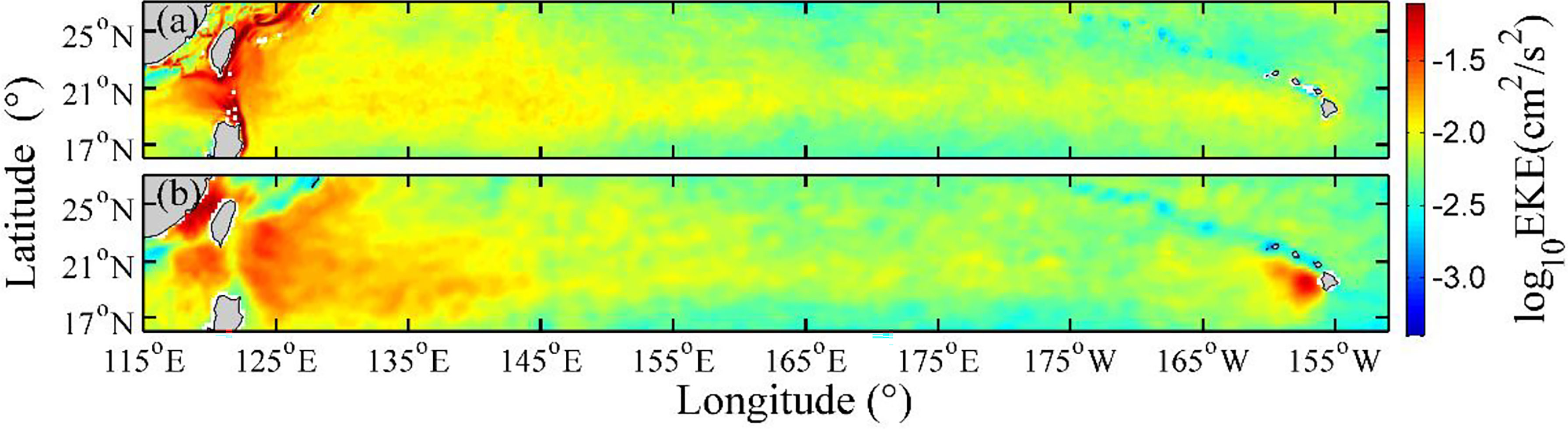
Figure 1 Distribution of sea surface eddy kinetic energy calculated from (A) OFES and (B) AVISO data. Shading indicates eddy kinetic energy (units: cm2/s2). Note that the eddy kinetic energy is plotted with log base 10.
Eddy detection and tracking algorithm
At present, there are many eddy automatic detection and tracking algorithms, such as “OW” (Okubo, 1970; Weiss, 1991) and “WA” methods (Sadarjoen and Post, 2000). This study adopts a vector geometry-based two-dimensional eddy detection scheme proposed by Nencioli et al. (2010). Compared with “OW” and “WA” methods, this method can obtain a higher detection success rate and lower excess detection rate. It has been successfully applied to the regional and global study of oceanic eddies, such as the STCC region (Liu et al., 2012), the Southern California Bight (Dong et al., 2012), the Madeira Islands (Couvelard et al., 2012), the Alboran Sea (Peliz et al., 2013), the Mediterranean (Aguiar et al., 2013), the South China Sea (Sun et al., 2018; Sun et al., 2021a), Kuroshio Extension region (Ji et al., 2018), East China Sea (Liu et al., 2017b), North Pacific Ocean (Sun et al., 2019), Indian Ocean (Wang et al., 2019), the Southern Ocean (Sun et al., 2021b), and the global ocean (Dong et al., 2014; Dong et al., 2022; You et al., 2022). Please refer to the supporting information (Text S1) for a detailed description of this method.
A three-dimensional eddy detection method (Dong et al., 2012) is also used in this paper. This method assumes that the same eddy meets the following three conditions at different depths: 1) the eddy occurrence time is the same; 2) the eddy polarity is the same; and 3) the position deviation of the eddy center between two adjacent layers is less than 1/4 of the eddy radius in the upper layer. This method can integrate the eddy information detected on the two-dimensional plane into three-dimensional eddy information. Please refer to the supporting information (Text S2) for a detailed description of the three-dimensional eddy automatic detection method.
Definition of four types of eddies
The definition of a normal eddy has been well known and accepted. The CCE (ACE) is defined as an eddy with an anticlockwise (clockwise) rotation flow field and an average temperature anomaly inside the eddy (T′eddy) of less than zero (larger than zero). However, there are several different viewpoints on the definition of the abnormal eddy. Sun et al. (2019) proposed that the abnormal eddy needs to meet the following conditions: 1) the average temperature inside the CWE (ACE) is 0.1°C warmer (colder) than the average temperature of the annular area between the CWE (ACE) boundary and 1.5 times the eddy boundary; 2) the proportion of the warm (cold) temperature points inside the CWE (ACE) is at least 60% of the total points. Liu et al. (2021) only used the positive and negative of the filtered temperature anomaly to define the abnormal eddy. In the global study of abnormal eddies, Ni et al. (2021) reported that defining abnormal eddies by using the difference between the temperature inside and around the eddies, and using the positive and negative temperature anomalies after filtering were statistically the same.
Therefore, this study uses a relatively simple definition of abnormal eddies. That is, according to the rotation direction of the eddy flow field and the average temperature anomaly inside the eddy (T′eddy), the mesoscale eddy is divided into four types: cyclonic cold-core eddy (CCE, with an anticlockwise rotation flow field and a negative T′eddy), anticyclonic warm-core eddy (AWE, with a clockwise rotation flow field and a positive T′eddy), cyclonic warm-core eddy (CWE, with an anticlockwise rotation flow field and a positive T′eddy), anticyclonic cold-core eddy (ACE, with a clockwise rotating flow field and a negative T′eddy). In this study, CCE and AWE are collectively referred to as normal eddies, while CWE and ACE are referred to as abnormal eddies.
Three additional constraints are added to the resulting three-dimensional eddy dataset to increase the robustness of the results. (1) Considering that the lifespan of mesoscale eddies is several weeks to several months, only eddies with a lifespan greater than or equal to 30 days are selected. (2) Regarding the spatial scale of mesoscale eddies and the spatial resolution of the OFES data, only eddies with an average radius larger than 25 km are retained. (3) Given the uncertainty of the simulation results in the deep ocean and the substantial standard deviation of the average eddy radius below 5,000 m, this study only discusses eddies above that depth.
Eddy cases analysis
Four eddy cases are presented in Figure 2 to understand the three-dimensional structure of the four types of eddies in the STCC region (please refer to Table 1 for a detailed description of these cases.). The gray shadow indicates the outer boundary of the eddy case, and the color indicates the temperature anomaly (T′) after high-pass space filtering. The vertical planes show the cross-section along the meridional and zonal direction through the eddy center.
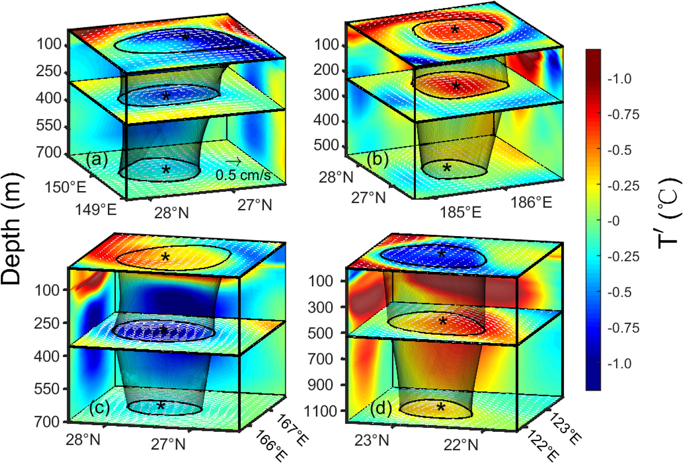
Figure 2 Three-dimensional structures of four types of eddy cases in the STCC region. (A–D) represent cyclonic cold-core eddy, anticyclonic warm-core eddy, cyclonic warm-core eddy, and anticyclonic cold-core eddy, respectively. The color and white vectors indicate the temperature anomaly (units: °C) and the velocity anomaly vector (units: cm/s) after high-pass space filtering. The black curves and the asterisk represent the eddy boundary and eddy center at the corresponding depth, respectively. The gray shadow represents the outer boundary of the eddy case. The vertical planes show the cross-section along the meridional and zonal directions through the eddy center.

Table 1 Basic information of the four types of eddy cases.
Figure 2A shows a CCE case on February 6, 2009. It formed on January 16, 2009, and died on March 1, 2009, with a lifespan of 48 days. Therefore, the figure shows the mature stage of this eddy (Liu et al., 2012). The eddy centers at its surface and bottom are located at (149.95°E, 27.25°N) and (149.85°E, 27.45°N), respectively. The central axis of this eddy is inclined by 24.33 km in the vertical direction. The average eddy radii of this CCE case on the surface, bottom, and overall depth are 65.00, 50.87, and 56.65 km, respectively. According to the classification of eddy shapes proposed by Lin et al. (2015), it is a bowl-shaped eddy. The vertical penetration depth of this eddy is 694.1 m. The maximum and average temperature anomalies induced by this eddy on the surface are -1.31°C and -0.67°C, respectively. The overall maximum eddy-induced temperature anomaly is -1.31°C, which occurs at 7.56 m.
Figure 2B shows the three-dimensional structure of an AWE case on April 21, 2013. It formed on March 10, 2013, died on June 23, 2013, and had a lifespan of 108 days. Therefore, the figure also shows the mature stage of the eddy lifespan. The eddy centers on the surface and bottom layer are located at (185.75°E, 27.45°N) and (185.65°E, 27.35°N), respectively, and the eddy central axis is inclined by 14.87 km in the vertical direction. The average radii of this eddy at the surface, bottom, and whole depth are 60.10, 70.16, and 51.93 km, respectively. Therefore, this AWE case belongs to a lens-shaped eddy. The vertical penetration depth of this eddy is 460.50 m. The maximum and average eddy-induced surface temperature anomalies are 0.74°C and 0.50°C, respectively. The maximum temperature anomaly caused by this eddy is 1.99°C, which occurs at 120.77 m.
Figure 2C shows the three-dimensional structure of a CWE case on January 25, 2010. This eddy was formed on October 27, 2009, and died on February 9, 2010, with a lifespan of 105 days. Therefore, the figure shows the decaying stage of the eddy. The eddy centers on the surface and the bottom layer are located at (166.75°E, 27.55°N) and (166.65°E, 27.55°N), respectively. That is, the central axis of this CWE tilts 9.86 km vertically. The average radii of this eddy are 58.48, 46.88, and 31.31 km at the surface, bottom, and overall depth, respectively. Therefore, like the CCE case, this eddy belongs to a bowl-shaped eddy as well. The vertical penetration depth of this eddy case is 700.00 m. The maximum and average surface temperature anomalies induced by this eddy are 0.58°C and 0.31°C, respectively. The maximum positive (negative) temperature anomaly caused by this CWE case is 1.74°C (-1.13°C), which occurs at 134.31 m (319.01 m).
Figure 2D shows the three-dimensional structure of an ACE case on January 7, 2010. This eddy formed on October 18, 2009, and died on January 28, 2010, with a lifespan of 99 days. Therefore, the figure shows the 81st day of the eddy lifespan, which is in the eddy decaying stage. The eddy centers on the surface and the bottom layer are both located at (122.55°E, 22.75°N), i.e., the central axis of this ACE is not tilted vertically. The average eddy radii are 65.30, 61.62, and 50.10 km at the surface, bottom and overall depth, respectively. Therefore, like the CCE and CWE cases, this eddy also belongs to a bowl-shaped eddy. The vertical penetration depth of this eddy is 1,185.00 m. The maximum and average surface temperature anomalies induced by the ACE are -0.93°C and -0.62°C, respectively. The maximum negative temperature anomaly induced by this ACE case is -0.93°C, which occurs at 95.56 m, while the maximum positive temperature anomaly is 1.41°C, which occurs at 357.60 m.
It can be seen that the abnormal eddy phenomenon is mainly concentrated in the ocean’s upper layer and become a normal eddy after reaching a certain depth (CWE case exceeds 223.20 m, ACE case exceeds 148.40 m). This result is consistent with the previous results from Sun et al. (2021a) and Ni et al. (2021).
Eddy statistical characteristics
Eddy numbers
There are two methods to count the number of mesoscale eddies (Yang et al., 2020). One is based on the eddy lifespan, called the lifespan counting (ELC) method. In this method, an eddy is counted as one throughout its lifespan. The other is the snapshot counting (ESC) method, in which the eddy number is the number of times the eddy is observed. For example, an eddy with a lifespan of 60 days will be observed 21 times because the temporal resolution of the OFES data is three days. According to the ELC method, the eddy number is 1, but according to the ESC method, the eddy number is 21. This study uses the ESC method, except when discussing the eddy movement direction.
Figure 3 shows the eddy number distribution of the four types of eddies in 1° by 1° grids to explore the uneven distribution of eddies at the sea surface. From 2008 to 2017, the total number of normal eddies is 143,965, of which 75,726 are CCEs, accounting for 52.60% (Figure 3A), and 68,239 are AWEs, accounting for 47.40% (Figure 3B). That is, there are 5.20% more CCEs than AWEs, which is consistent with the statistical results of Liu et al. (2012) using satellite altimeter measurement data (CEs are 6.95% more than AEs). The total number of abnormal eddies is 68,751, of which 27,554 and 41,197 are CWEs and ACEs, accounting for 40.08% and 59.92%, respectively. The number of ACEs is 19.84% more than that of CWEs. Regarding spatial distribution, normal eddies are mainly distributed in the open ocean (Figures 3A, B). In contrast, abnormal eddies are primarily distributed in the southeast of the STCC region, the South China Sea, and near the Hawaiian Islands (Figures 3C, D).
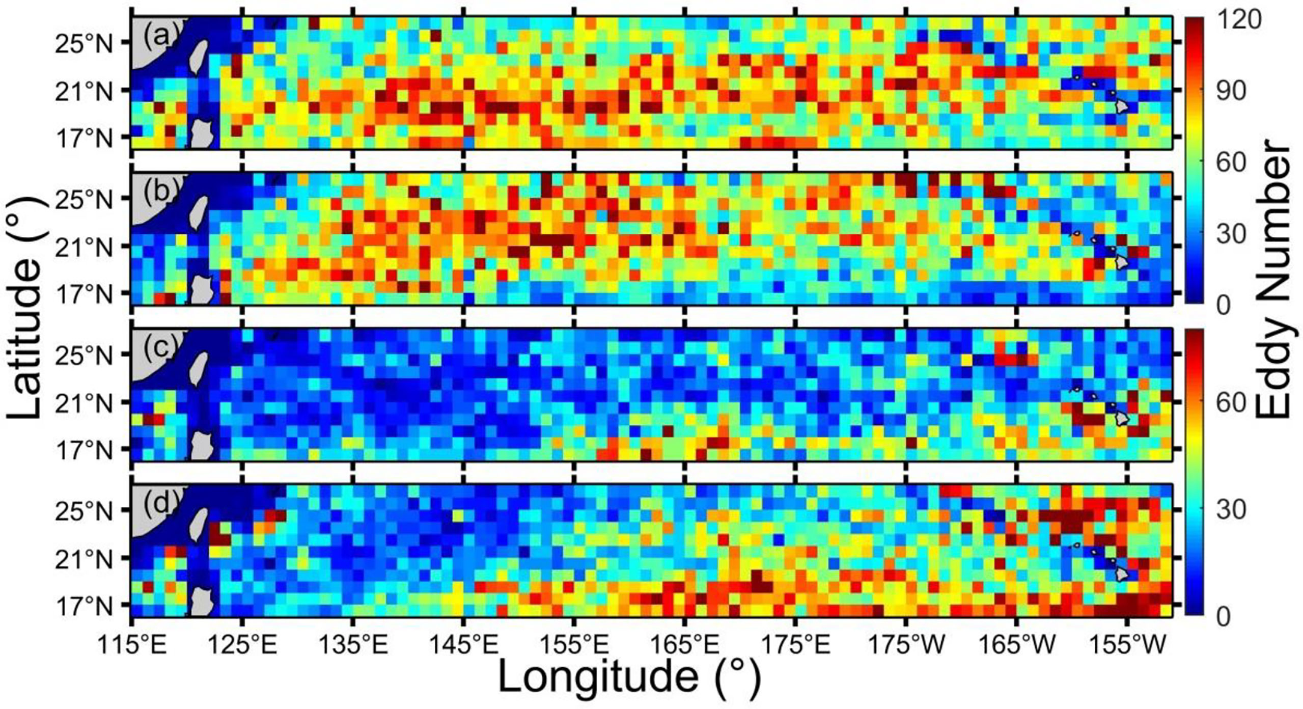
Figure 3 Number of four types of eddies at the sea surface in the STCC region in each 1° by 1° grid. (A–D) show cyclonic cold-core eddy, anticyclonic warm-core eddy, cyclonic warm-core eddy, and anticyclonic cold-core eddy, respectively. The color indicates the number of eddies. Note that (A, B) and (C, D) use different color bar ranges.
In Figure 3A, the CCEs are concentrated in the range of 18 ~ 21°N. The eddy numbers in the boundary region of STCC are much less than that in the middle area. In Figure 3B, the AWEs are mainly distributed between 20 and 22°N. If the CCEs and AWEs are combined (i.e., considering total normal eddies), their concentration area is 19 ~ 22°N. This spatial distribution is more southerly than the result (eddy mainly concentrated in the 22 ~ 23°N band area) of Hwang et al. (2004), and the different data used may cause this difference. CWEs are concentrated along 20°N and from 160 to 155°W bands near the Hawaiian Islands (Figure 3C). ACEs are mainly concentrated in the southeast part of the STCC region and the northern region of the Hawaiian Islands (Figure 3D).
The above analysis shows that the high incidence area of CCEs (AWEs) is the low-value area of CWEs (ACEs). On the contrary, the low-value area CCEs (AWEs) is the high incidence area of CWEs (ACEs).
Figure 4 shows the vertical distribution of the four types of eddies. Comparing Figure 4A with B, the number of normal and abnormal eddies has the opposite change trend in the vertical direction. However, the change trend within the normal and abnormal eddies is almost identical. Specifically, in the upper 1,000 m, the number of CCEs and AWEs gradually increases with depth, decreases between 1,000 and 4,000 m, and eventually increases below 4,000 m (Figure 4A). On the contrary, the number of CWEs and ACEs first decreases in the upper 1,000 m, then gradually increases with depth between 1,000 and 4,000 m, and finally decreases below 4,000 m (Figure 4B).
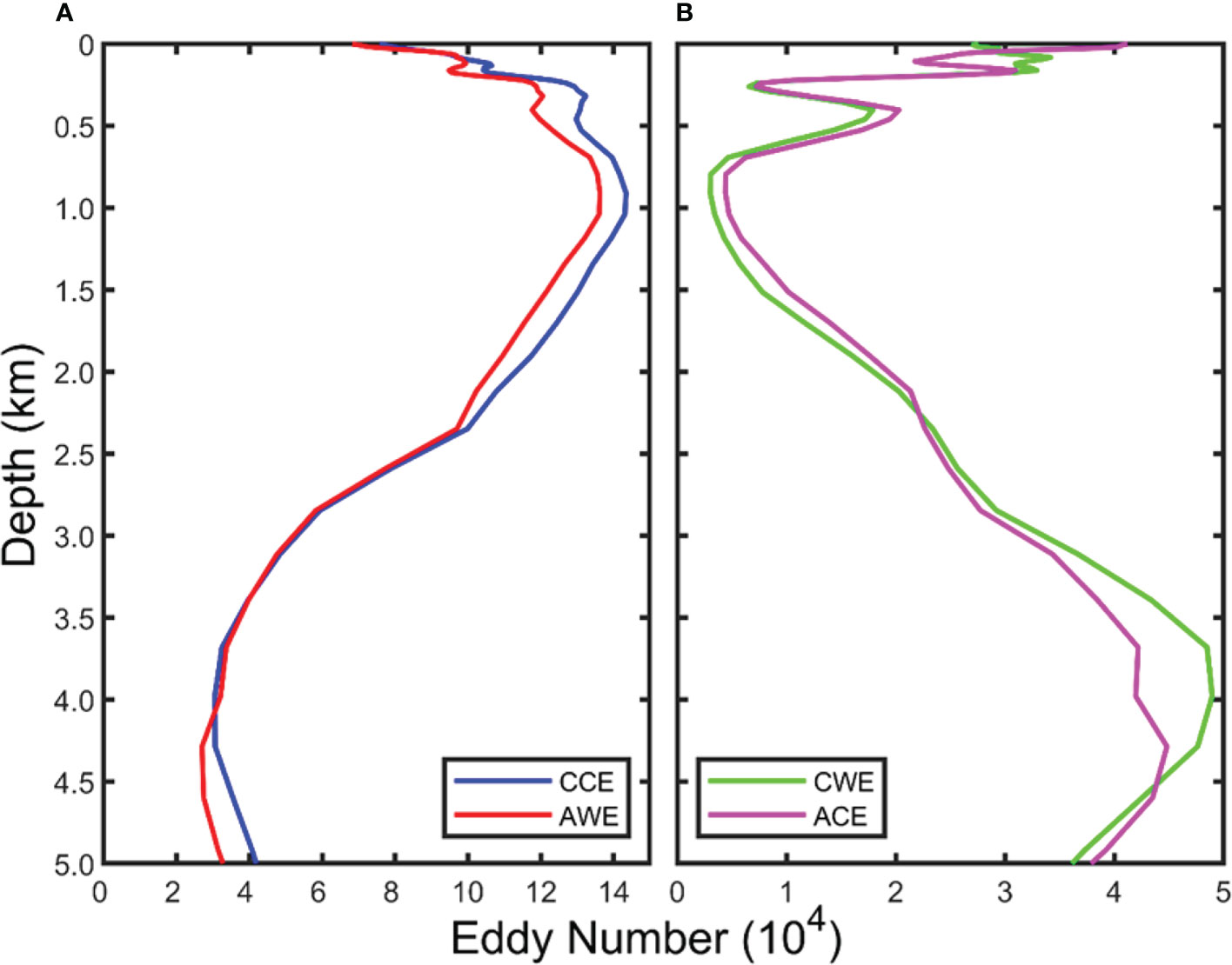
Figure 4 Vertical distribution of four types of eddies’ number in the STCC region. Blue, red, green, and magenta curves represent cyclonic cold-core eddy (A), anticyclonic warm-core eddy (A), cyclonic warm-core eddy (B), and, anticyclonic cold-core eddy (B), respectively.
The number of normal eddies at the surface is 2.09 times that of abnormal eddies (143,965 for normal eddies and 68,751 for abnormal eddies). At about 3,300 m, the number of normal and abnormal eddies is almost equal, and then the number of abnormal eddies exceeds that of normal eddies at deeper layers. The apparent increase in abnormal eddies below 1,000 m may be due to their definition. The present study does not limit the temperature difference between the eddy interior and surrounding background field to 0.1°C, as suggested by Sun et al. (2019). As a result, many eddies with very small temperature anomalies below 1,000 m are classified as abnormal eddies. If the strict definition of abnormal eddies in Sun et al. (2019) is adopted, the number of abnormal eddies below 1,000 m will sharply reduce (figure not shown).
Eddy radius
The average distance from the eddy boundary to the eddy center is defined as the eddy radius in this study (please refer to S1 in the supporting information for a comparison of four types of eddy radii). The statistical histogram of eddy average radius at the surface (Figures 5A, B) and 1,000 m (Figures 5C, D) is given in Figure 5. The ordinate γ1 indicates the percentage of eddies in a particular bin relative to the total number of eddies with the same type. In the figure, an eddy radius smaller (larger) than 40 km (120 km) is placed in the 25 ~ 40 km (120 ~ 130 km) bin.
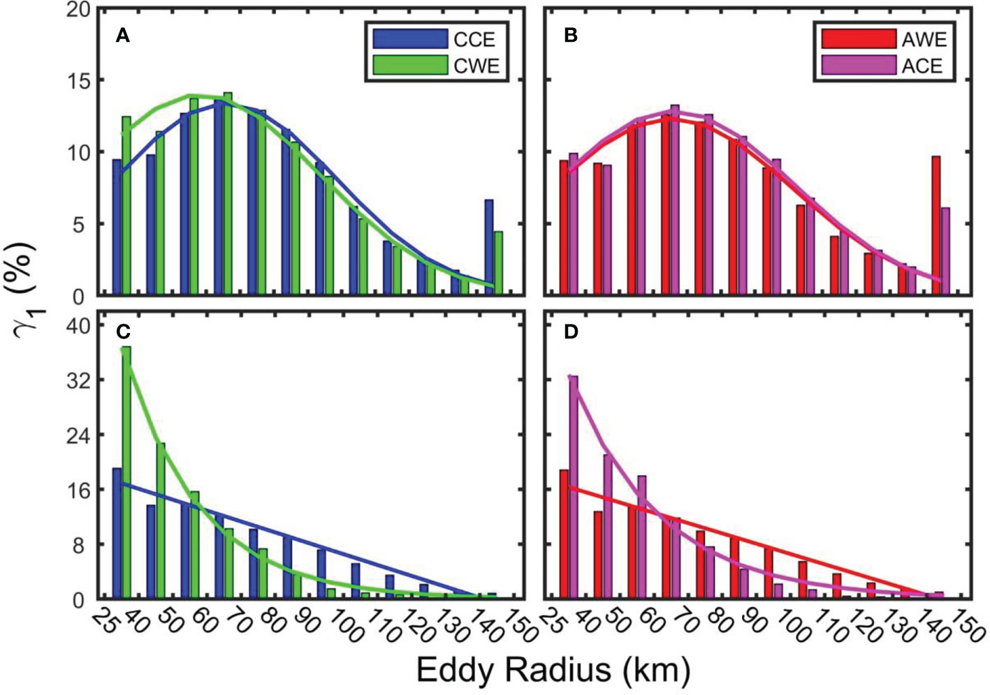
Figure 5 Statistical histogram of eddy radius at the sea surface (A, B) and 1,000 m (C, D). Blue, red, green, and magenta curves represent cyclonic cold-core eddy, anticyclonic warm-core eddy, cyclonic warm-core eddy, and anticyclonic cold-core eddy, respectively.
The average radius of CCEs, AWEs, CWEs, and ACEs at the surface layer is 79.14 ± 3.7, 83.34 ± 3.75, 73.74 ± 4.14, and 79.46 ± 3.89 km, respectively. At 1,000 m, the average radius of the four types of eddies is 68.35 ± 4.76, 70.40 ± 5.37, 49.32 ± 8.15, and 51.33 ± 7.48 km. The result of the average eddy radius at the surface layer is slightly smaller than that pointed out by Tang et al. (2019), in which the average radius of CE is 91 km and AE 94 km. The main reason for this difference may be that the spatial resolution of the satellite altimeter data used by Tang et al. (2019) is 1/4° by 1/4°, while the OFES data is 1/10° by 1/10°. In addition, the average eddy radius at 1,000 m is significantly smaller than that of the surface layer.
From Figure 5A, the eddy radius of the CCEs and CWEs has a Gaussian distribution (i.e. , where α , μ and σ means the undetermined coefficient, average value and the standard deviation, respectively.), and the expression of the fitting function is for CCEs and for CWEs. It can be concluded from comparing the average and standard deviation of the two Gaussian fitting functions that the eddy radius of CCEs is more significant than that of CWEs, and its distribution is also more concentrated than that of CWEs. The maximum statistical probability of the average radius of CCEs and CWEs lies within 60 ~ 70 km. Among them are 10,334 CCEs, accounting for 13.64% of the total CCEs, and 3,885 CWEs, accounting for 14.10% of the total CWEs. The maximum eddy radius of CCEs and CWEs is 396 and 340 km, respectively.
Figure 5B shows that the statistical distribution of the AWEs and ACEs radius also follows a Gaussian distribution, and the expressions of their fitting function are and , respectively. It can be seen from the fitting functions that the average radius of ACEs is more significant than that of AWEs, and the distribution of eddy radius is more concentrated than that of AWEs. The maximum statistical probability of the average radius for AWEs and ACEs is also 60 ~ 70 km. Among them are 8,573 AWEs, 12.57% of the total AWEs, and 5,450 ACEs, accounting for 13.23% of the total ACEs. The maximum radius of the AWEs and ACEs are 429 and 370 km, respectively.
It is evident from Figure 5C that the statistical probability distribution of CCE radius almost decreases linearly at 1,000 m, and its linear fitting function is . The maximum statistical probability of the average CCE radius is 25 ~ 40 km. There are 27,301 CCEs in this bin, accounting for 19.08% of the total CCEs. The statistical probability of the CWE radius decreases exponentially, and the fitting function is . The maximum statistical probability of the average CWE radius is 25 ~ 40 km. There are 1,259 CWEs in this bin, accounting for 36.81% of the total CWEs. The maximum radius of the CCEs and CWEs is 334 and 253 km, respectively.
From Figure 5D, the radius probability distribution of the AWEs decreases linearly at 1,000 m, and its linear fitting function is . The maximum statistical probability of the average AWE radius is 25 ~ 40 km, which includes 25,574 eddies, accounting for 18.80% of the total AWEs. The ACE radius probability distribution is in the form of exponential decay, and the fitting function is . The maximum statistical probability of the average ACE radius is 25 ~ 40 km, which is the same as AWEs. There are 1,537 ACEs in this section, accounting for 32.46% of the total ACEs. The maximum radius of the AWE and ACE are 360 and 226 km, respectively.
At 1,000 m, the fitting functions of the eddy radius probability of CCEs and AWEs are linear functions, while the fitting functions for CWEs and ACEs are exponential functions, indicating that the eddy radius of abnormal eddies phenomenon is more likely to occur in the smaller eddies.
All four types of eddies have their largest average radius in the surface layer (Figure 6). The surface average radius of AE (81.40 km) is 6.09% larger than that of CE (76.44 km). This result is consistent with the statistical finding of Liu et al. (2012) using altimeter data. The variation trend of the normal eddies average radius in the vertical direction is more stable than that of abnormal eddies. The normal eddies average radius decreases by 18 km (from 79.1 to 61.1 km) from the surface to 1,500 m. From 1,500 to 5,000 m, the eddy radius decreases by only 11 km (from 61.1 to 50.1 km). The overall trend of the average abnormal eddy radius from surface to 1,000 m also decreases, then increases slightly from 1,000 m to 2,000 m. Below 2,000 m, the average radius of the abnormal eddy remains stable at about 52 km.
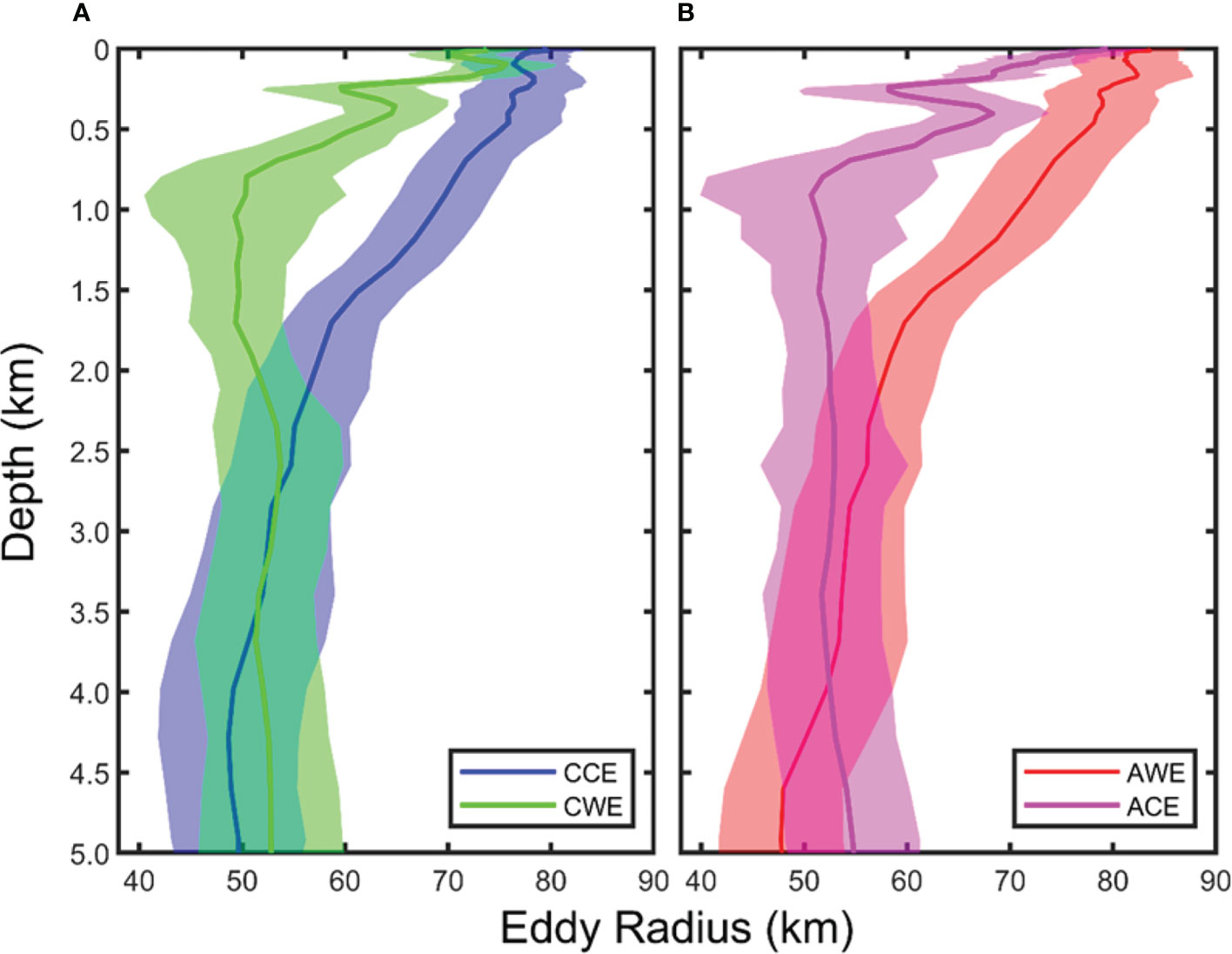
Figure 6 Vertical distribution of the average eddy radius from the four types of eddies in the STCC region. Blue, red, green, and magenta curves represent the average radius of cyclonic cold-core eddy (A), anticyclonic warm-core eddy (B), cyclonic warm-core eddy (A), and anticyclonic cold-core eddy (B), respectively (units: km). The shaded area represents the standard deviation of the corresponding eddy’s average radius.
Eddy amplitude
The eddy amplitude is defined as the absolute value of the sea surface height anomaly (SSHA) extremum within the eddy (please refer to S2 in the supporting information for a comparison of four types of eddies’ amplitude). From Figure 7, it is found that the average eddy amplitude of CCEs, AWEs, CWEs, and ACEs is 3.25 ± 2.78, 3.28 ± 2.51, 2.85 ± 2.56, and 3.02 ± 2.40 cm, respectively. This value is much smaller than the average amplitude of global eddies (about 8 cm) pointed out by Chelton et al. (2011). The median (maximum) value of eddy amplitude for CCEs, AWEs, CWEs, and ACEs is 3.31 (20.10), 3.02 (20.62), 3.27 (20.58), and 2.96 (20.80) cm, respectively. The median of CEs is larger than that of AEs, but their maximum amplitudes are very close. The ordinate γ2 indicates the percentage of eddies in a particular bin relative to the total number of eddies with the same type (Figure 7). The statistical histograms of the four types of eddy amplitudes follow a Gaussian distribution, and their fitting functions are: for CCEs, for AWEs, for CWEs, and for AWEs, respectively. The order of the amplitude concentration of the four types of eddies is ACEs, AWEs, CWEs, and CCEs, and the amplitude distribution concentration of the AEs is higher than that of CEs.
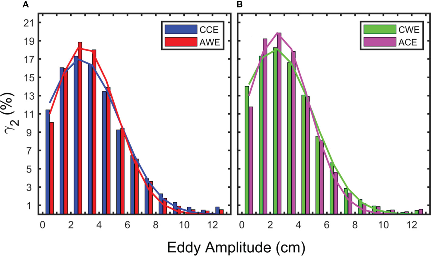
Figure 7 Statistical histogram of eddy amplitude for the four types of eddies. Blue, red, green, and magenta bars represent cyclonic cold-core eddy (A), cyclonic warm-core eddy (B), anticyclonic warm-core eddy (A), and anticyclonic cold-core eddy (B), respectively. The curves in the figure show the distribution of the Gaussian fitting function.
The maximum probability distribution of eddy amplitudes for CCEs, AWEs, CWEs, and ACEs are all concentrated at the 2 ~ 3 cm bin, reaching 13,108 (17.31%), 12,863 (18.85%), 5,029 (18.25%), and 8,182 (19.86%), respectively. The amplitude of CCEs, AWEs, CWEs, and ACEs less than 5 cm reaches 56,559 (74.69%), 52,408 (76.80%), 21,845 (79.28%), and 33,600 (81.56%), respectively, which is higher than the 40% reported by Chelton et al. (2011). Accordingly, the number of eddies with an amplitude larger than 10 cm is 1,598 (2.11%), 983 (1.44%), 306 (1.11%), and 564 (1.37%), respectively, which is less than the 25% reported by Chelton et al. (2011). The reasons for this difference deserve further discussion in future studies.
Eddy eccentricity
Based on satellite data, Hwang et al. (2004) pointed out that the shape of eddies in the STCC region is mainly elliptical. Using in-situ observation from an underwater glider, Qiu et al. (2019) found an AWE with an irregular shape. In this study, we perform ellipse fitting on the eddy boundary and take the ellipse’s eccentricity as an index to measure the irregularity of the eddy. According to the definition of elliptical eccentricity, it varies between 0 and 1. The smaller the eddy eccentricity is, the closer the eddy is to a circle. Accordingly, the larger the eddy eccentricity is, the flatter the eddy is. Please refer to Table S3 in the supporting information for the comparison information of the four types of eddy eccentricities.
The statistical histogram of eddy eccentricity is shown in Figure 8, where the ordinate γ3 is the ratio of the eddy number in the corresponding interval to the total of the corresponding eddy type. The eddy eccentricities show a partial Gaussian distribution, and their fitting functions of CCEs, AWEs, CWEs, and ACEs at the surface are , , , and , respectively. From the expression of the fitting function, it can be seen that there is no noticeable difference in the eccentricity of the four types of eddies.
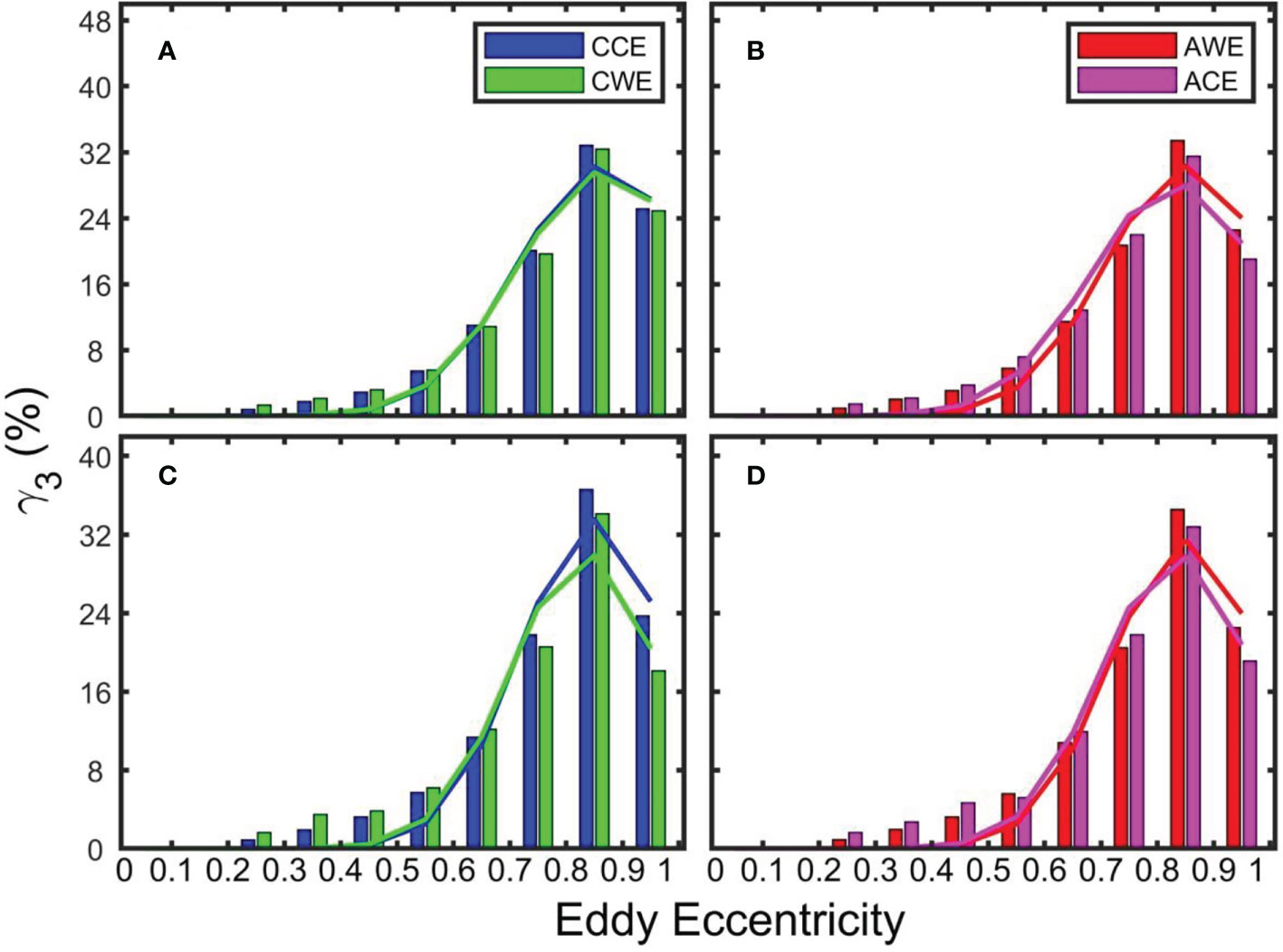
Figure 8 Statistical histogram of eddy eccentricity at the sea surface (A, B) and 1,000 m (C, D). Blue, red, green, and magenta bars represent cyclonic cold-core eddy, anticyclonic warm-core eddy, cyclonic warm-core eddy, and anticyclonic cold-core eddy, respectively. The curves show the distribution of the Gaussian fitting function.
The average eccentricity of CCEs, AWEs, CWEs, and ACEs at the sea surface is 0.76 ± 0.35, 0.76 ± 0.33, 0.73 ± 0.50, and 0.73 ± 0.73 (Figures 8A, B). Accordingly, the corresponding average eddy eccentricity at 1,000 m is 0.76 ± 1.58, 0.76 ± 1.69, 0.73 ± 1.73, and 0.66 ± 3.28, respectively (Figures 8C, D). The average eddy eccentricity of normal eddies (0.76) is 4.11% larger than that of abnormal eddies (0.73). However, the standard deviation of the abnormal eddy eccentricity is about twice that of normal eddy eccentricity, indicating that the eccentricity of abnormal eddies is more dispersed.
The eddy eccentricity distribution of the four types of eddies at the surface and 1,000 m is mostly in the range of 0.8 ~ 0.9 (Figure 8). At the sea surface, there are 24,887 (32.86%) CCEs, 22,780 (33.40%) AWEs, 8,911(32.34%) CWEs, and 12,969 (31.48%) ACEs, which are in the 0.8 ~ 0.9 bin. There are only a few eddies with an eccentricity less than 0.2 at the sea surface, including 196 (0.26%) CCEs, 79 (0.12%) AWEs, 40 (0.15%) CWEs, and 63 (0.15%) ACEs, indicating that almost-circular eddies rarely exist in the ocean. At 1,000 m, there are 52,355 (36.59%) CCEs, 46,972 (34.53%) AWEs, 1,166 (34.09%) CWEs, 1,553 (32.80%) ACEs in the 0.8 ~ 0.9 bin. There are few eddies with an eddy eccentricity less than 0.2 at 1,000 m, including 155 (0.11%) CCEs, 152 (0.11%) AWEs, 2 (0.06%) CWEs, and 13 (0.27%) ACEs, indicating that almost-circular eddies rarely exist at 1,000 m as well.
In a word, the eccentricity probability distributions of the four types of eddies at the surface and 1,000 m are all in the range of 0.8 ~ 0.9, corresponding to the maximum value. There are only a few eddies with eccentricity less than 0.2.
Figure 9 shows the vertical distribution of the four types of eddies’ eccentricity. The average eccentricity of normal eddies fluctuates slightly within the upper 1,000 m and gradually decreases from 1,000 to 5,000 m. In contrast, abnormal eddies show a decreasing trend within the upper 1,000 m and with large fluctuations. Below 1,000 m, the eddy eccentricity of CWEs decreases, while the ACEs’ eccentricity gradually increases above 2,000 m and then almost remains stable. Overall, the eccentricity of the abnormal eddies is smaller than that of the normal eddies, especially in the ocean’s upper layer.
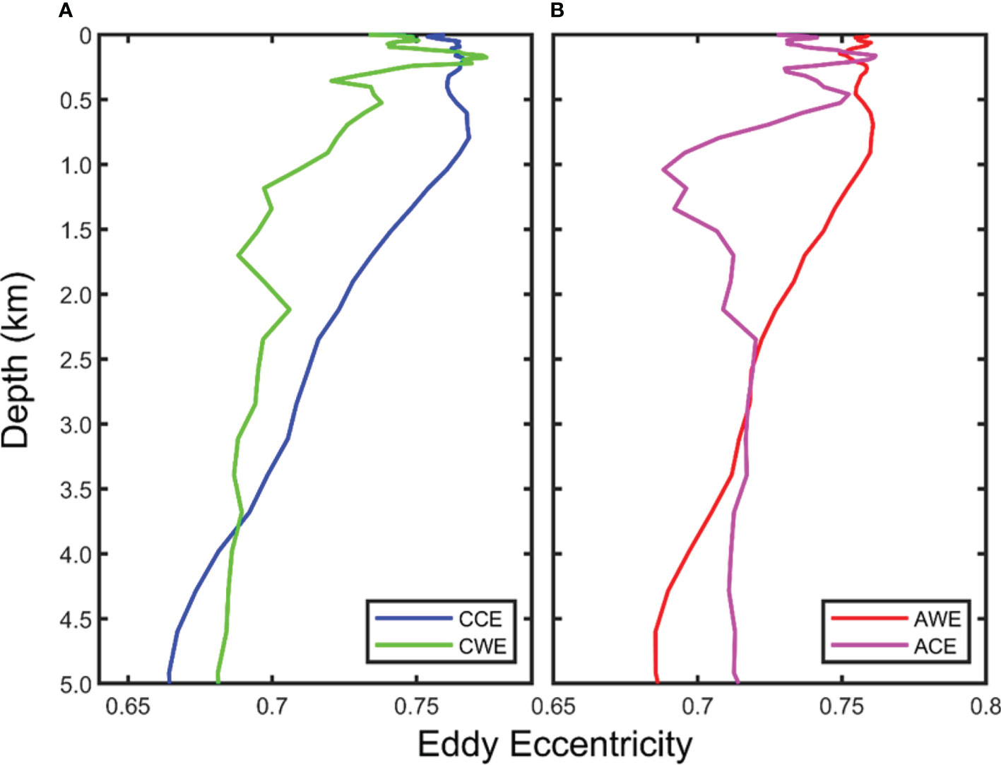
Figure 9 Vertical distribution of the average eddy eccentricity of the four types of eddies in the STCC region. Blue, red, green, and magenta curves represent cyclonic cold-core eddy (A), anticyclonic warm-core eddy (B), cyclonic warm-core eddy (A), and anticyclonic cold-core eddy (B), respectively.
The maximum eddy eccentricity for CCE, AWE, CWE, and AWE is 0.77, 0.77, 0.78, and 0.77, occurring at 796.38, 694.09, 192.50, and 148.35 m, respectively. Accordingly, the minimum eddy eccentricity for CCEs, AWEs, CWEs, and AWEs is 0.66, 0.68, 0.65, and 0.66, which occurs at 4,600.00, 4,286.51, 1,515.41, and 1,041.39 m, respectively. The average eccentricity of the four types of eddies decreases in the vertical direction, but the variation range is minimal (CCE: 0.12, AWE: 0.09, CWE: 0.13, and ACE: 0.11).
Eddy movement direction
Previous studies showed that eddies move westward in a zonal direction on a global scale (Chelton et al., 2011). However, eddy movement in the meridional direction is different. Some studies point out that most CEs move poleward while AEs move equatorward (Chelton et al., 2007). Based on satellite altimeter data from 1993 to 2010, Liu et al. (2012) pointed out that in the STCC region, both CEs and AEs generated south (north) of 21°N would be deflected northward (southward). The first view does not limit the area of eddy generation (south or north of 21°N), but it limits the type of eddies (CE or AE). In contrast, the second view does not limit the type of eddy but the area where it is generated. Based on the following two considerations, we continue to use the traditional division method in this subsection and only divide the eddy into CEs and AEs. On the one hand, this allows for comparison with the results from previous studies. On the other hand, to discuss the eddy movement trajectory, it is necessary to treat the whole eddy lifespan as one eddy. Previous studies have shown that in the whole lifespan of the eddy, there will be a situation where one stage belongs to the normal eddy, and another stage belongs to the abnormal eddy (Sun et al., 2019). Therefore, if we continue to divide the eddies into four types, the eddies at different lifespan stages may be divided into two or more eddies, so it is impossible to calculate the deflection direction of their movement.
The trajectory of eddies (with a lifespan longer than 30 days) and their frequency distribution in the STCC region are given in Figure 10 (please refer to Table S4 in the supporting information for information on eddy movement direction). We move the eddy generation position to the origin in the figure and specify the eastward and northward directions as positive. During the study period, there are 3,598 eddies with a lifespan of more than 30 days generated north of 21°N, including 1,741 CEs and 1,857 AEs (Figure 10A). On the whole, eddies move westward. The longest distance of CEs and AEs in the zonal direction is -25.40° (~ 2,636.75 km) and -50.30° (~ 5,221.60 km), respectively, and the average distance is -2.07 ± 2.90° (~ 214.88 ± 301.05 km) and -2.91 ± 4.60° (~ 302.08 ± 477.52 km). The maximum deflection distance of CEs and AEs to the north is 5.90° (612.47 km) and 6.40° (664.38 km), respectively. The maximum deflection distance to the south is -7.00° (726.66 km) and -8.30° (861.60 km), and the average deflection distance is -0.16 ± 1.17° (16.61 ± 121.46 km) and -0.07 ± 1.29° (7.27 ± 133.91 km). The average deflection distance in the meridional direction is about 4.70% of that in the zonal direction, which indicates that the horizontal transport of substances (such as nutrients) by eddies is mainly concentrated in the zonal direction. However, considering that the temperature of the seawater presents a belt-like distribution in the zonal direction, the eddy-induced heat transport in the zonal and meridional directions needs to be specifically analyzed. The statistical histogram shows that 51.20% (45.64%) of eddies move southward (northward), including 52.44% (44.11%) of CEs and 50.03% (47.07%) of AEs (Figure 10B). The remaining 3.16% of eddies (3.45% CEs and 2.91% AEs) do not deflect north or south.
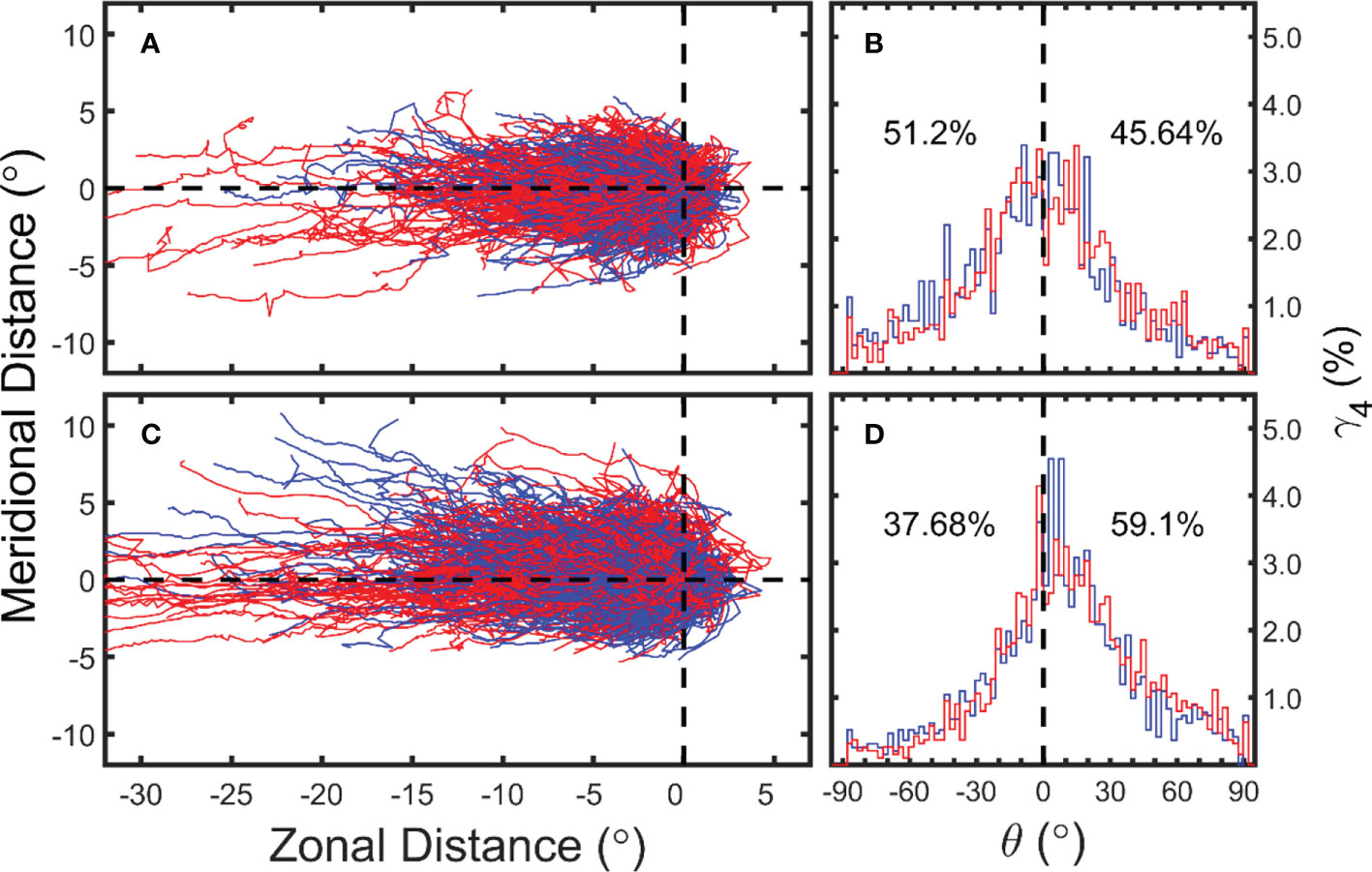
Figure 10 Trajectories of eddies generated (A) north and (C) south of 21°N in the STCC region at the sea surface. East and North directions are positive, and the West and South are negative. (B) and (D) show the statistical histogram of eddy trajectory deflection azimuth. Blue and red indicate CEs and AEs, respectively.
Accordingly, there are 3,922 eddies generated south of 21°N, including 1,991 CEs and 1,931 AEs (Figure 10C). The longest moving distance of CEs and AEs in the zonal direction is -44.50° (4,619.51 km) and -61.20° (6,353.12 km), respectively, and the average moving distance is -3.12 ± 4.22° (323.88 ± 438.07 km) and -3.56 ± 5.77° (369.56 ± 598.98 km). The maximum deflection distance of CEs and AEs to the north is 10.80° (1,198.8 km) and 9.90° (1,098.9 km), respectively, while the maximum deflection distance to the south is -5.20° (577.20 km) and -5.30° (588.3 km). The average deflection distance to the south is 0.36 ± 1.51° (39.96 ± 167.61 km) and 0.48 ± 1.47° (53.28 ± 163.17 km) for CEs and AEs, respectively. Among these eddies, 59.10% (37.68%) of the eddy trajectories have a northward (southward) deflection, including 57.86% (38.32%) CEs and 60.39% (37.03%) AEs. The remaining 3.16% of the eddy trajectories (3.82% CEs and 2.59% AEs) do not deflect north or south. These results agree with Liu et al. (2012). Following the method of Chelton et al. (2007), 51.94% of CEs and 53.32% of AEs deflect to the north, and 44.38% of CEs and 44.00% of AEs deflect to the south. Accordingly, 3.68% of CEs and 2.68% of AEs will not deflect in the meridional direction (figure not shown).
Eddy velocity
Figure 11 shows the statistical histogram of the averaged zonal (Figures 11A–D) and meridional (Figures 11E–H) eddy velocity component at the surface (Figures 11A, B, E, F) and 1,000 m (Figures 11C, D, G, H). The ordinate represents the ratio of eddy number in the corresponding interval to the total number of the same type of eddies. The maximum zonal velocity of CCEs, AWEs, CWEs, and ACEs at the surface is -49.64, -49.67, -49.66, and -49.65 cm/s, and the average value is -4.29 ± 0.92, -3.97 ± 2.30, -4.05 ± 1.06, and -4.93 ± 1.61 cm/s, respectively. Accordingly, 51.71, 53.47, 52.38, and 48.37% of the eddies have a zonal velocity less than 5 cm/s, while only 5.20, 5.83, 5.20, and 5.70% of the eddies have zonal velocities of more than 20 cm/s. The Gaussian fitting functions corresponding to the statistical histogram of the eddy zonal velocity for the four types of eddies at the surface are , , and , respectively. The fitting functions for the four types of eddies are only different in the undetermined coefficient α, and the other two parameters (μ and σ) are identical, indicating that there is no apparent difference among the four types of eddies in this respect.
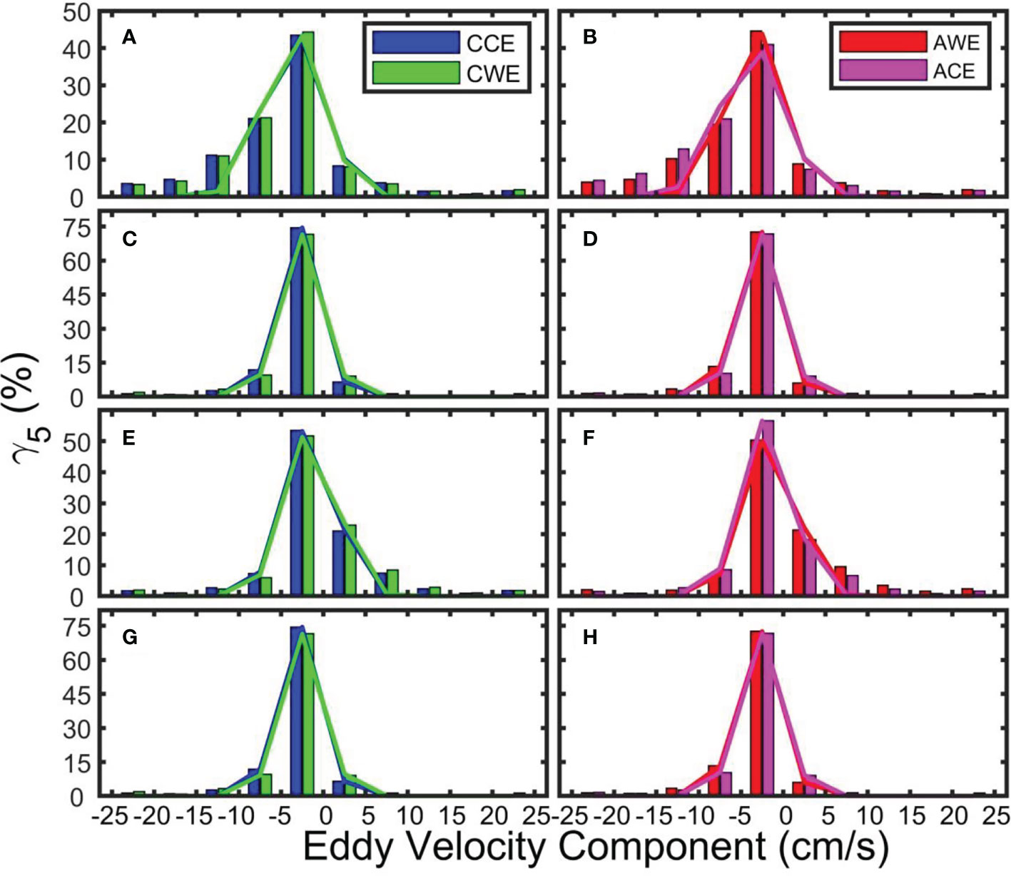
Figure 11 Statistical histogram of zonal (A–D) and meridional (E–H) eddy velocity at the sea surface (A, B, E, F) and at 1,000 m (C, D, G, H, units: cm/s). Blue, red, green, and magenta bars represent cyclonic cold-core eddy, cyclonic warm-core eddy, anticyclonic warm-core eddy, and anticyclonic cold-core eddy, respectively. Eastward and northward are positive, and westward and southward are negative. The curves show the distribution of the Gaussian fitting function.
The maximum zonal velocity of CCEs, AWEs, CWEs and ACEs at 1,000 m is -49.72, -49.69, -49.52, and -49.55 cm/s, and the average velocity is -2.78 ± 1.23, -3.11 ± 1.25, -2.04 ± 4.56, and -2.06 ± 4.15 cm/s, respectively (Figure 11C, D). Accordingly, 80.97, 78.62, 80.64, and 80.76% of the eddies move at a zonal velocity less than 5 cm/s, while only 1.91, 1.93, 3.22, and 2.88% of the eddies have a zonal velocity of more than 20 cm/s at 1,000 m. The expressions of the Gaussian fitting function cor to the statistical histogram of the eddy zonal velocity for the four types of eddies at 1,000 m are , , , and , respectively. Since μ in the fitting function is equal to zero, it can be inferred that the eddy zonal velocity at a depth of 1,000 m is almost zero. Comparing Figures 11A–D, the magnitude of the eddy zonal velocity at 1,000 m is significantly smaller than that at the surface. Its average magnitude is only 0.65, 0.78, 0.50, and 0.42% that at the surface layer, respectively.
The maximum meridional velocity of CCEs, AWEs, CWEs, and ACEs at the surface is -49.73, -49.52, -49.69, and -49.55 cm/s, while the average value is 0.11 ± 1.04, 0.85 ± 2.50, 0.49 ± 1.70, and 0.39 ± 1.67 cm/s respectively. Among these eddies, 74.50, 71.72, 74.60, and 74.86% have a meridional velocity less than 5 cm/s, while only 3.56, 4.43, 3.75, and 3.18% have a meridional velocity larger than 20 cm/s. The Gaussian fitting functions corresponding to the statistical histogram of the meridional velocity for the four types of eddies at the sea surface are , , , and , respectively. Similar to the zonal velocity’s fitting functions, the meridional velocity’s fitting functions are also almost identical.
Accordingly, at 1,000 m, the maximum meridional velocity of CCEs, AWEs, CWEs, and ACEs is -49.73, -49.52, -49.69, and -49.55 cm/s, and their average value is -0.13 ± 1.55, -0.06 ± 1.54, -0.35 ± 5.00, and -0.22 ± 3.65 cm/s, respectively. Among these four types of eddies, 80.97, 78.62, 80.64, and 80.76% have meridional velocity less than 5 cm/s, while only 1.91, 1.93, 3.22, and 2.88% are larger than 20 cm/s. The expressions of the Gaussian fitting function corresponding to the statistical histogram of the eddy meridional velocity for the four types of eddies at 1,000 m are , , and , respectively. Similar to the zonal velocity’s fitting functions at 1,000 m, μ in the fitting function is also equal to zero, indicating no meridional movement trend of the eddies at 1,000 m. For the comparison information of the four types of eddies’ velocity, please refer to Table S5 in the supporting information.
Figure 12 shows the vertical distribution of eddy velocity and the average background field velocity. The four types of eddies move westward (negative zonal velocity) in the overall water depth, and the size of the zonal eddy velocity is larger than that of the background field (Figures 12A–D). Below 700 m, the average zonal velocity of the background field is almost zero, which makes the difference in zonal velocity size between the eddy and the background field more obvious. The zonal velocity of the four types of eddies increases with depth in the upper 1,000 m. It first increases rapidly, then decreases gradually, and finally tends to be stable. Even in the deep ocean (nearly 5,000 m), the eddy zonal velocity does not reach zero but remains at about -1.3 cm/s.
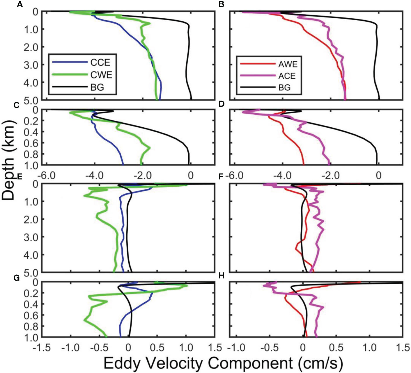
Figure 12 Vertical distribution of eddy zonal (A–D) and meridional (E–H) velocity component (units: cm/s). Blue, red, green, magenta, and black curves represent the eddy velocity component of cyclonic cold-core eddy, anticyclonic warm-core eddy, cyclonic warm-core eddy, anticyclonic cold-core eddy and multi-year average background field, respectively.
The maximum average zonal velocity of CCEs, AWEs, CWEs, and ACEs is -4.29, -4.58, -5.02, and -5.65 cm/s, appearing at 2.50, 120.77, 65.23, and 54.02 m, respectively. Figures 12C, D show the distribution in the upper 1,000 m to make the vertical change of the zonal velocity clearer. The figures show that in the upper ocean (CWE corresponds to 200 m, and the ACE corresponds to about 170 m), the zonal velocity of abnormal eddies is greater than that of normal eddies. Deeper than that, the zonal velocity of the abnormal eddies is significantly smaller than that of the normal eddies until the velocity difference between the two almost disappears below 2,500 m.
The eddy meridional velocity has noticeable changes (especially for the normal eddy) within the upper 1,000 m, and its size is very small and has little difference below 1,000 m (Figures 12E–H). The maximum meridional velocity for CCEs, AWEs, CWEs, and ACEs is 0.42, 0.86, 1.01, and -0.59 cm/s, respectively, appearing at 207.50, 7.56, 73.23, and 73.23 m. Figures 12G, H show that in the upper 100 m, CEs (CCEs and CWEs) and AWEs deflect northward, while ACEs deflect southward. The value of the background meridional velocity changes rapidly and decreases sharply from nearly 2 cm/s to almost 0 at 55 m in the ocean’s upper layer. This meridional velocity increases slightly from 55 to 108 m and gradually decreases below 108 m, finally remaining almost stable below 700 m, showing a northward direction, but the size is nearly zero.
Eddy nonlinearity
Ocean eddies can transport heat and freshwater horizontally. Many studies attribute it to the fact that an eddy is nonlinear and can trap seawater. Therefore, the degree of eddy nonlinearity can measure its ability to transport freshwater and other substances. According to Chelton et al. (2011), we define eddy nonlinearity as , where v1 and v2 are the eddy average rotation velocity and the eddy movement velocity in the horizontal direction, respectively. Eddy nonlinearity larger than one means the eddy rotation velocity exceeds its horizontal movement velocity. The eddy has the ability to enclose materials within the eddy and transport it horizontally. On the contrary, eddy nonlinearity less than one means the eddy rotation velocity is less than the horizontal movement velocity. Therefore, the ability to trap materials within the eddy is weak, and it is not easy to transport materials horizontally. For the comparison information of the four types of eddies’ nonlinearity, please refer to Table S6 in the supporting information.
Figure 13 shows the statistical horizontal nonlinearity distribution of the four types of eddies at the surface (Figures 13A, B) and 1,000 m (Figure 13C, D). There are 42,407, 37,375, 13,424, and 18,963 eddies with a nonlinearity larger than one at the surface, accounting for 56.00, 54.77, 48.72, and 46.03% of CCEs, AWEs, CWEs, and ACEs, respectively. The expressions of the Gaussian fitting function corresponding to the eddy nonlinearity statistical histogram of the four types of eddies are , , , and , respectively. From the four fitting functions, the coefficient μfor the normal eddy is larger than that in the abnormal eddy, indicating that the normal eddy is stronger than the abnormal eddy in the eddy nonlinearity. This result also verifies the view that abnormal eddies mainly occur in eddies’ generation and decay stages (with weak nonlinearity, Sun et al., 2019).
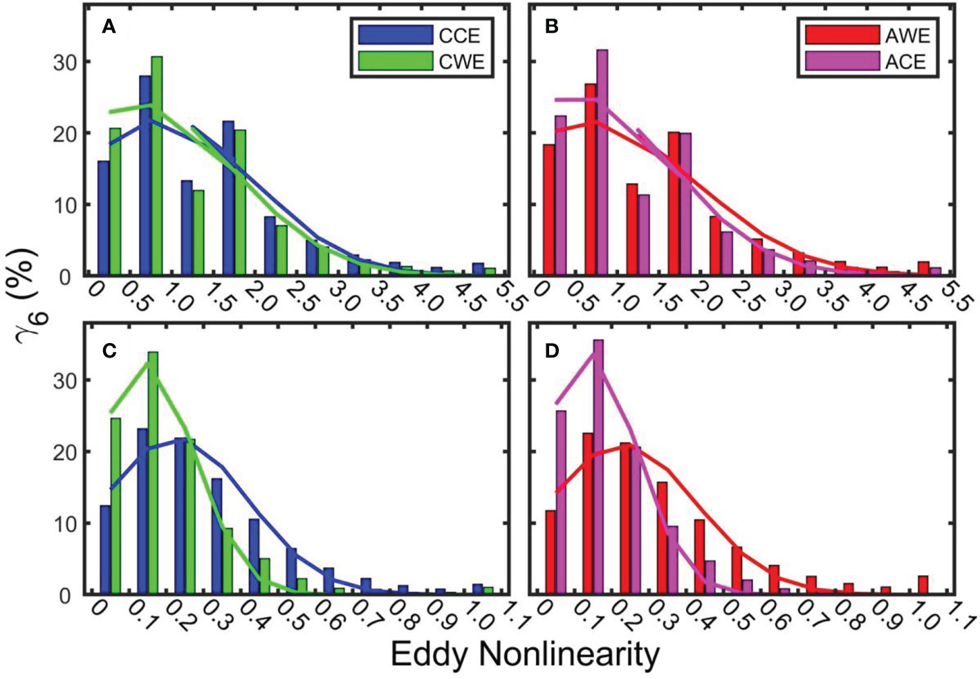
Figure 13 Statistical histogram of eddy nonlinearity at the surface (A, B) and 1,000 m (C, D). Blue, red, green, and magenta bars represent cyclonic cold-core eddy, anticyclonic warm-core eddy, cyclonic warm-core eddy, and anticyclonic cold-core eddy, respectively. The curves show the distribution of the Gaussian fitting function.
Accordingly, among the four types of eddies at 1,000 m, there are 1,068, 1,767, 284, and 74 eddies with an eddy nonlinearity larger than one, accounting for 1.41, 2.59, 1.03, and 0.18% of the corresponding types of eddies. The expressions of the Gaussian fitting functions corresponding to the eddy nonlinearity statistical histogram for the four types of eddies are , , , , respectively. As in the case on the sea surface, the normal eddies’ nonlinearity is also more substantial than the abnormal eddies at 1,000 m.
Figure 14 shows the vertical distribution of the average eddy nonlinearity of the four types of eddies. The average eddy nonlinearity decreases rapidly with depth in the upper 1,000 m, and the rate of change becomes very small below that depth. The maximum average eddy nonlinearity of the four types of eddies appears at the surface layer. The maximum value for CCEs, AWEs, CWEs, and ACEs is 1.3925, 1.3911, 1.2249, and 1.1769, respectively. The minimum average eddy nonlinearity corresponding to the four types of eddies is 0.1842, 0.1796, 0.1712, and 0.1672, respectively, which appears at 2,847.0, 2,847.0, 1,515.4, and 2,348.9 m. The depth of CCEs, AWEs, CWEs, and ACEs with average eddy nonlinearity larger than one is concentrated in the ocean’s upper layer, which is 109.0, 116.0, 159.0, and 52.0 m, respectively. Below this depth, their nonlinearities become less than one.
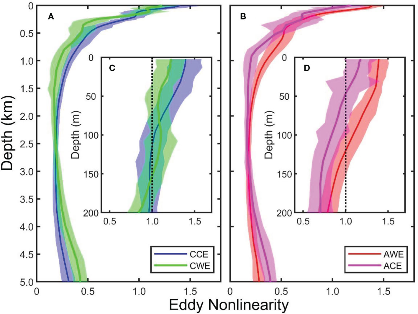
Figure 14 Vertical distribution of eddy nonlinearity from the four types of eddies. Blue, red, green, and magenta represent cyclonic cold-core eddy, anticyclonic warm-core eddy, cyclonic warm-core eddy, and anticyclonic cold-core eddy, respectively. The shaded areas represent the corresponding standard deviation. (A) represents the vertical profiles of cyclonic cold-core eddy and cyclonic warm-core eddy, and (B) represents the vertical profiles of anticyclonic cold-core eddy and anticyclonic warm-core eddy. (C) and (D) are enlarged images of the upper 200 m layer of (A, B), respectively.
Conclusions
The STCC region is the second highest EKE region in the North Pacific Ocean. This area is rich in mesoscale eddy activities and various mesoscale eddy types. This study uses the newly proposed eddy classification method to divide mesoscale eddies into four categories: CCEs with anticlockwise rotating flow field and cold eddy core, AWEs with clockwise rotating flow field and warm eddy core, CWEs with anticlockwise rotating flow field and warm eddy core, and ACEs with clockwise rotating flow field and cold eddy core.
The spatial characteristics of these four kinds of mesoscale eddies are discussed in detail based on the OFES data. The analysis of four eddy cases shows that the eddy in the STCC region has bowl-shaped and lens-shaped three-dimensional structures. The abnormal eddy phenomenon mainly occurs in the ocean’s upper layer. After a certain depth, the abnormal eddy often goes back to a normal eddy.
Based on the eddy detection results of OFES data from 2008 to 2017, the statistical analysis shows that the proportion of the four types of eddies at the sea surface is 35.60, 32.08, 12.95, and 19.37%, respectively. Regarding the spatial distribution at the sea surface, normal eddies are primarily distributed in the open ocean. In contrast, abnormal eddies are mainly distributed southeast of the STCC, the South China Sea, and the Hawaiian Islands. The maximum number of normal eddies in the vertical direction appears at 1,000 m, indicating a considerable number of subsurface eddies in the ocean (Assassi et al., 2016, Nan et al., 2017), which is a scientific problem worthy of further study.
The average radius of the four types of eddies at the sea surface is almost the same (about 80 km). However, at a depth of 1,000 m, the average radius of the normal and abnormal eddies is about 70 and 50 km, respectively. In the vertical direction, the maximum average radius of the four types of eddies appears at the sea surface, which confirms the view of Lin et al. (2015) that most oceanic eddies have a bowl-shaped structure.
The average amplitude of the four types of eddies in the STCC area is only about 3 cm, less than half of the global statistical result (~ 8 cm) obtained by Chelton et al. (2011). Among the four types of eddies, the proportion of eddies with an amplitude larger than 10 cm is less than 3%, which is much less than the result of 25% reported by Chelton et al. (2011). Most of the four types of eddies’ eccentricity occur in the range of 0.8 ~ 0.9, indicating that most eddies are elliptic-shaped. Only a few eddies’ eccentricities are less than 0.2. In the vertical direction, the eccentricity of the four types of eddies shows a decreasing trend with depth.
Regarding the horizontal movement direction of eddies, except for the apparent westward movement characteristics, the eddies generated north of 21°N tend to deflect to the south, while eddies generated south of 21°N tend to deflect to the north. The average zonal velocity of the four kinds of eddies at the sea surface is -4.29 ± 0.92, -3.97 ± 2.30, -4.05 ± 1.06, and -4.93 ± 1.61 cm/s, respectively. Accordingly, 51.71, 53.47, 52.38, and 48.37% of the eddies have a zonal velocity less than 5 cm/s, while only 5.20, 5.83, 5.20, and 5.70% of the eddies have zonal velocities of more than 20 cm/s. Accordingly, the average meridional velocity is 0.11 ± 1.04, 0.85 ± 2.50, 0.49 ± 1.70, and -0.39 ± 1.67 cm/s respectively. Among these eddies, 74.50, 71.72, 74.60, and 74.86% have meridional velocity less than 5 cm/s, while only 3.56, 4.43, 3.75, and 3.18% are larger than 20 cm/s.
According to the definition of eddy nonlinearity in Chelton et al. (2011), this study finds that strongly nonlinear eddies are mostly distributed in the ocean’s upper layer, and nearly half are larger than one. However, at a depth of 1,000 m, the ratio is only 1.41, 2.59, 1.03, and 0.18%, respectively.
A detailed discussion of the spatial distribution characteristics of the four types of eddies helps deepen the understanding of the mesoscale eddy phenomenon in the STCC region. The STCC region is located in the East Asian monsoon-dominated region, and the mesoscale eddy activities in this area will inevitably be affected by the seasonal changes in the atmospheric background field. The seasonal difference in eddy characteristics is one of the current scientific problems we are discussing. In addition, the possible generation mechanism of abnormal eddies and whether this abnormal eddy phenomenon is regionally dependent will discuss in a future study.
Data availability statement
The original contributions presented in the study are included in the article/Supplementary Material. Further inquiries can be directed to the corresponding author.
Author contributions
WS, YL, and CD conceived and designed the experiments. WS performed the experiments. WS, MA, JieL, JisL, WT, and JJ analyzed the data. WS and MA drafted the original manuscript. WS, CD, KS, and JY revised and edited the manuscript. All authors contributed to the article and approved the submitted version.
Funding
National Natural Science Foundation of China under contract Nos. 41906008, 42192562, 42076162, 42176012; Open Fund of State Key Laboratory of Satellite Ocean Environment Dynamics, Second Institute of Oceanography, MNR under contract No. QNHX2231; Natural Science Foundation of Guangdong Province of China under contract No. 2020A1515010496; and Innovation Group Project of Southern Marine Science and Engineering Guangdong Laboratory (Zhuhai) under contract No. 311020004.
Acknowledgments
The OFES simulation was conducted on the Earth Simulator under the support of JAMSTEC. This data is downloaded from http://apdrc.soest.hawaii.edu/ (Data DOI: https://doi.org/10.17596/0002029). The altimeter products are produced by the Ssalto/Duacs and distributed by AVISO, with support from the Centre National d’Etudes Spatiales (http://www.aviso.oceanobs.com/duacs/).
Conflict of interest
The authors declare that the research was conducted in the absence of any commercial or financial relationships that could be construed as a potential conflict of interest.
Publisher’s note
All claims expressed in this article are solely those of the authors and do not necessarily represent those of their affiliated organizations, or those of the publisher, the editors and the reviewers. Any product that may be evaluated in this article, or claim that may be made by its manufacturer, is not guaranteed or endorsed by the publisher.
Supplementary Material
The Supplementary Material for this article can be found online at: https://www.frontiersin.org/articles/10.3389/fmars.2022.1004300/full#supplementary-material
References
Aguiar A. C. B., Peliz Á., Carton X. (2013). A census of meddies in a long-term high-resolution simulation. Prog. Oceanogr. 116 (9), 80–94. doi: 10.1016/j.pocean.2013.06.016
Assassi C., Morel Y., Vandermeirsch F., Chaigneau A., Pegliasco C., Morrow R., et al. (2016). An index to distinguish surface- and subsurface-intensified vortices from surface observations. J. Phys. Oceanogr. 46 (8), 2529–2552. doi: 10.1175/JPO-D-15-0122.1
Bashmachnikov I., Boutov D., Dias J. (2013). Manifestation of two meddies in altimetry and sea-surface temperature. Ocean Sci. 9 (2), 249–259. doi: 10.5194/os-9-249-2013
Chang Y. L., Oey L. Y. (2014). Analysis of STCC eddies using the okubo–Weiss parameter on model and satellite data. Ocean Dyn. 64 (2), 259–271. doi: 10.1007/s10236-013-0680-7
Chelton D. B., Schlax M. G., Samelson R. M. (2011). Global observations of nonlinear mesoscale eddies. Prog. Oceanogr. 91 (2), 167–216. doi: 10.1016/j.pocean.2011.01.002
Chelton D. B., Schlax M. G., Samelson R. M., De Szoeke R. A. (2007). Global observations of large oceanic eddies. Geophys. Res. Lett. 34 (L15606), 87–101. doi: 10.1029/2007GL030812
Chen G., Yang J., Han G. (2021). Eddy morphology: Egg-like shape, overall spinning, and oceanographic implications. Remote Sens. Environ. 257, 112348. doi: 10.1016/j.rse.2021.112348
Chow C. H., Tseng Y., Hsu H., Young C. (2017). Interannual variability of the subtropical countercurrent eddies in the north pacific associated with the Western-pacific teleconnection pattern. Cont. Shelf Res. 143, 175–184. doi: 10.1016/j.csr.2016.08.006
Couvelard X., Caldeira R. M. A., Araújo I. B., Tomé R. (2012). Wind mediated vorticity-generation and eddy-confinement, leeward of the Madeira island: 2008 numerical case study. Dyn. Atmos. Oceans. 58 (6), 128–149. doi: 10.1016/j.dynatmoce.2012.09.005
Dawson H. R. S., Strutton P. G., Gaube P. (2018). The unusual surface chlorophyll signatures of southern ocean eddies. J. Geophys. Res. 123 (9), 6053–6069. doi: 10.1029/2017JC013628
Dong C., Lin X., Liu Y., Nencioli F., Chao Y., Guan Y., et al. (2012). Three-dimensional oceanic eddy analysis in the southern California bight from a numerical product. J. Geophys. Res. 117, 92–99. doi: 10.1029/2011JC007354
Dong C., Liu L., Nencioli F., Bethel B. J., Liu Y., Xu G., et al. (2022). The near-global ocean mesoscale eddy atmospheric-oceanic-biological interaction observational dataset. Sci. Data. 9 9, 436. doi: 10.1038/s41597-022-01550-9
Dong C., Mcwilliams J. C., Liu Y., Chen D. (2014). Global heat and salt transports by eddy movement. Nat. Commun. 5 (2), 1–6. doi: 10.1038/ncomms4294
Ellwood M. J., Strzepek R. F., Strutton P. G., Trull T. W., Fourquez M., Boyd P. W. (2020). Distinct iron cycling in a southern ocean eddy. Nat. Commun. 11, 825. doi: 10.1038/s41467-020-14464-0
Frenger I., Gruber N., Knutti R., Münnich M. (2013). Imprint of southern ocean eddies on winds, clouds and rainfall. Nat. Geosci. 6 (8), 608–612. doi: 10.1038/NGEO1863
Frenger I., Münnich M., Gruber N., Knutti R. (2015). Southern ocean eddy phenomenology. J. Geophys. Res. 120 (11), 7413–7449. doi: 10.1002/2015JC011047
He Q., Zhan H., Cai S. (2020). Anticyclonic eddies enhance the winter barrier layer and surface cooling in the bay of bengal. J. Geophysical Research: Oceans 125 (10), e2020J–e16524J. doi: 10.1029/2020JC016524
He Q., Zhan H., Cai S., He Y., Huang G., Zhan W. (2018). A new assessment of mesoscale eddies in the south China Sea: Surface features, three-dimensional structures, and thermohaline transports. J. Geophys. Res. 123, 4906–4929. doi: 10.1029/2018JC014054
Hosoda K., Hanawa K. (2004). Anticyclonic eddy revealing low sea surface temperature in the sea south of Japan: Case study of the eddy observed in 1999–2000. J. Oceanogr. 60 (4), 663–671. doi: 10.1007/s10872-004-5759-9
Hu H., Zhao Y., Zhang N., Bai H., Chen F. (2021). Local and remote forcing effects of oceanic eddies in the subtropical front zone on the mid-latitude atmosphere in winter. Clim. Dynam. 57 (11-12), 3447–3464. doi: 10.1007/s00382-021-05877-8
Hwang C., Wu C. R., Kao R. (2004). TOPEX/Poseidon observations of mesoscale eddies over the subtropical countercurrent: Kinematic characteristics of an anticyclonic eddy and a cyclonic eddy. J. Geophys. Res. 109 (C08013), 371–375. doi: 10.1029/2003JC002026
Itoh S., Yasuda I. (2010). Water mass structure of warm and cold anticyclonic eddies in the western boundary region of the subarctic north pacific. J. Phys. Oceanogr. 40 (12), 2624–2642. doi: 10.1175/2010JPO4475.1
Ji J., Dong C., Zhang B., Liu Y. (2016). Oceanic eddy statistical comparison using multiple observational data in the kuroshio extension region. Acta Oceanol. Sin. 36 (3), 1–7. doi: 10.1007/s13131-016-0882-1
Ji J., Dong C., Zhang B., Liu Y., Zou B., Gregory P. K., et al. (2018). An oceanic eddy characteristics and generation mechanisms in the kuroshio extension region. J. Geophys. Res. 123, 2018J–2123J. doi: 10.1029/2018JC014196
Kang L., Wang F., Chen Y. L. (2010). Eddy generation and evolution in the north pacific subtropical countercurrent (NPSC) zone. Chin. J. Oceanology Limnol. 28 (5), 968–973. doi: 10.1007/s00343-010-9010-9
Lian Z., Wei Z., Wang Y., Wang X. (2021). Geographical variation and controlling mechanism of eddy-induced vertical temperature anomalies and eddy available potential energy in the south China Sea. Ocean Dynam. 71 (4), 411–421. doi: 10.1007/s10236-021-01441-4
Lin X., Dong C., Chen D., Liu Y., Yang J., Zou B., et al. (2015). Three-dimensional properties of mesoscale eddies in the south China Sea based on eddy-resolving model output. Deep Sea Res. 99, 46–64. doi: 10.1016/j.dsr.2015.01.007
Li Q., Sun L., Xu C. (2018). The lateral eddy viscosity derived from the decay of oceanic mesoscale eddies. Open J. Mar. Sci. 08 (01), 152–172. doi: 10.4236/ojms.2018.81008
Liu Y., Dong C., Guan Y., Chen D., Mcwilliams J., Nencioli F. (2012). Eddy analysis in the subtropical zonal band of the north pacific ocean. Deep Sea Res. 68 (5), 54–67. doi: 10.1016/j.dsr.2012.06.001
Liu Y., Dong C., Liu X., Dong J. (2017b). Antisymmetry of oceanic eddies across the kuroshio over a shelf break. Sci. Rep. 7 (1), 6761. doi: 10.1038/s41598-017-07059-1
Liu S., Sun L., Wu Q., Yang Y. (2017a). The responses of cyclonic and anticyclonic eddies to typhoon forcing: The vertical temperature-salinity structure changes associated with the horizontal convergence/divergence. J. Geophys. Res. 122 (6), 4974–4989. doi: 10.1002/2017JC012814
Liu Y., Zheng Q., Li X. (2021). Characteristics of global ocean abnormal mesoscale eddies derived from the fusion of sea surface height and temperature data by deep learning. Geophys. Res. Lett. 48 (17), e2021GL094772. doi: 10.1029/2021GL094772
Lu J., Wang F., Liu H., Lin P. (2016). Stationary mesoscale eddies, up-gradient eddy fluxes and the anisotropy of eddy diffusivity. Geophys. Res. Lett. 43, 743–751. doi: 10.1002/2015GL067384
Ma L., Wang Q. (2014a). Interannual variations in energy conversion and interaction between the mesoscale eddy field and mean flow in the kuroshio south of Japan. Chin. J. Oceanol. Limn. 32 (1), 210–222. doi: 10.1007/s00343-014-3036-3
Ma L., Wang Q. (2014b). Mean properties of mesoscale eddies in the kuroshio recirculation region. Chin. J. Oceanol. Limn. 32 (3), 681–702. doi: 10.1007/s00343-014-3029-2
McGillicuddy D. J. Jr. (2015). Formation of intrathermocline lenses by eddy–wind interaction. J. Phys. Oceanogr. 45 (2), 606–612. doi: 10.1175/JPO-D-14-0221.1
Nan F., Yu F., Wei C., Ren Q., Fan C. (2017). Observations of an extra-Large subsurface anticyclonic eddy in the northwestern pacific subtropical gyre. J. Mar. Sci. Res. Dev. 07 (04), 1000235. doi: 10.4172/2155-9910.1000234
Nencioli F., Dong C., Dickey T., Washburn L., Mcwilliams J. C. (2010). And its application to a high-resolution numerical model product and high-frequency radar surface velocities in the southern California bight. J. Atmos. Oceanic Technol. 27 (27), 564–579. doi: 10.1175/2009JTECHO725.1
Ni Q., Zhai X., Jiang X., Chen D. (2021). Abundant cold anticyclonic eddies and warm cyclonic eddies in the global ocean. J. Phys. Oceanogr. 51 (9), 2793–2806. doi: 10.1175/JPO-D-21-0010.1
Okubo A. (1970). Horizontal dispersion of floatable particles in the vicinity of velocity singularities such as convergences. Deep Sea Res. 17, 445–454. doi: 10.1016/0011-7471(70)90059-8
Peliz A., Boutov D., Teles-Machado A. (2013). The alboran Sea mesoscale in a long term high resolution simulation: Statistical analysis. Ocean Modell. 72 (12), 32–52. doi: 10.1016/j.ocemod.2013.07.002
Qi Y., Mao H., Du Y., Li X., Zhou Y., Xu K., et al. (2022). A lens-shaped, cold-core anticyclonic surface eddy in the northern south China Sea. Front. Mar. Sci. 9, 976273. doi: 10.3389/fmars.2022.976273
Qiu C., Yi Z., Su D., Wu Z., Liu H., Lin P., et al. (2022). Cross-slope heat and salt transport induced by slope intrusion eddy’s horizontal asymmetry in the northern south China Sea. J. Geophys. Res. doi: 10.1029/2022JC018406
Qiu B., Chen S. (2010). Interannual variability of the north pacific subtropical countercurrent and its associated mesoscale eddy field. J. Phys. Oceanogr. 40, 213–225. doi: 10.1175/2009JPO4285.1
Qiu C., Liang H., Huang Y., Mao H., Yu J., Wang D., et al. (2020). Development of double cyclonic mesoscale eddies at around xisha islands observed by a ‘Sea-whale 2000’ autonomous underwater vehicle. Appl. Ocean Res. 101, 102270. doi: 10.1016/j.apor.2020.102270
Qiu C., Liang H., Sun X., Mao H., Wang D., Yi Z., et al. (2021). Extreme Sea-surface cooling induced by eddy heat advection during tropical cyclonic in the north western pacific ocean. Front. Mar. Sci. 8. doi: 10.3389/fmars.2021.726306
Qiu C., Mao H., Wang Y., Yu J., Su D., Lian S. (2019). An irregularly shaped warm eddy observed by Chinese underwater gliders. J. Oceanogr. 75 (2), 139–148. doi: 10.1007/s10872-018-0490-0
Sadarjoen I. A., Post F. H. (2000). Detection, quantification, and tracking of vortices using streamline geometry. Comput. Graphics. 24 (3), 333–341. doi: 10.1016/S0097-8493(00)00029-7
Sandalyuk N. V., Bosse A., Belonenko T. V. (2020). The 3d structure of mesoscale eddies in the lofoten basin of the Norwegian Sea: A composite analysis from altimetry and in situ data. J. Geophys. Res. 125 (10), e2020JC016331. doi: 10.1029/2020JC016331
Sasaki H., Nonaka M., Masumoto Y., Sasai Y., Uehara H., Sakuma H. (2008). “An eddy-resolving hind cast simulation of the quasi-global ocean from 1950 to 2003 on the earth simulator,” in High resolution numerical modelling of the atmosphere and ocean. Eds. Hamilton K., Ohfuchi W. (New York: Springer), 157–185.
Su D., Lin P., Mao H., Wu J., Liu H., Cui Y., et al. (2020). Features of slope intrusion mesoscale eddies in the northern south China Sea. J. Geophys. Res. 125, e2019J–e15349J. doi: 10.1029/2019JC015349
Sun W., An M., Liu J., Liu J., Yang J., Tan W., et al. (2022). Comparative analysis of four types of mesoscale eddies in the kuroshio-oyashio extension region. Front. Mar. Sci. 9, 984244. doi: 10.3389/fmars.2022.0984244
Sun W., Dong C., Tan W., He Y. (2019). Statistical characteristics of cyclonic warm-core eddies and anticyclonic cold-core eddies in the north pacific based on remote sensing data. Remote Sens. 11 (2), 208. doi: 10.3390/rs11020208
Sun W., Dong C., Tan W., Liu Y., He Y., Wang J. (2018). Vertical structure anomalies of oceanic eddies and eddy-induced transports in the south China Sea. Remote Sens 10, 795. doi: 10.3390/rs10050795
Sun W., Dong C., Wang R., Liu Y., Yu K. (2017). Vertical structure anomalies of oceanic eddies in the kuroshio extension region. J. Geophys. Res. 122 (2), 1476–1496. doi: 10.1002/2016JC012226
Sun W., Liu Y., Chen G., Tan W., Lin X., Guan Y., et al. (2021a). Three-dimensional properties of mesoscale cyclonic warm-core and anticyclonic cold-core eddies in the south China Sea. Acta Oceanol. Sin. 40 (10), 17–29. doi: 10.1007/s13131-021-1770-x
Sun W., Yang J., Tan W., Liu Y., Zhao B., He Y., et al. (2021b). Eddy diffusivity and coherent mesoscale eddy analysis in the southern ocean. Acta Oceanol. Sin. 40 (10), 1–16. doi: 10.1007/s13131-021-1881-4
Sun J., Zhang S., Nowotarski C. J., Jiang Y. (2020). Atmospheric responses to mesoscale oceanic eddies in the winter and summer north pacific subtropical countercurrent region. Atmosphere 11 (8), 816. doi: 10.3390/atmos11080816
Taguchi B., Qiu B., Nonaka M., Sasaki H., Xie S., Schneider N. (2010). Decadal variability of the kuroshio extension: Mesoscale eddies and recirculations. Ocean Dynam. 60 (3), 673–691. doi: 10.1007/s10236-010-0295-1
Tang B., Hou Y., Yin Y., Po H. (2019). Statistical characteristics of mesoscale eddies and the distribution in the north pacific subtropical countercurrent. Oceanologia Limnologia Sin. 50 (5), 937–947. doi: 10.11693/hyhz20190300050
Treguier A. M., Lique C., Deshayes J., Molines J. M. (2017). The north Atlantic eddy heat transport and its relation with the vertical tilting of the gulf stream axis. J. Phys. Oceanogr. 47 (6), 1281–1289. doi: 10.1175/JPO-D-16-0172.1
Wang Z., Li Q., Sun L., Li S., Yang Y., Liu S. (2015). The most typical shape of oceanic mesoscale eddies from global satellite sea level observations. Front. Earth Sci. 9 (2), 202–208. doi: 10.1007/s11707-014-0478-z
Wang Q., Zeng L., Li J., Chen J., Yunkai H., JingLong Y., et al. (2018). Observed cross-shelf flow induced by mesoscale eddies in the northern south China Sea. J. Phys. Oceanogr. 48 (7), 1609–1628. doi: 10.1175/JPO-D-17-0180.1
Wang S., Zhu W., Ma J., Ji J., Yang J., Dong C. (2019). Variability of the great whirl and its impacts on atmospheric processes. Remote sens. 11 (3), 322. doi: 10.3390/rs11030322
Weiss J. (1991). The dynamics of enstrophy transfer in two-dimensional hydrodynamics. Physica D. 48, 273–294. doi: 10.1016/0167-2789(91)90088-Q
Xian T., Sun L., Yang Y., Fu Y. (2012). Monsoon and eddy forcing of chlorophyll-a variation in the northeast south China Sea. Int. J. Remote Sens. 33 (23), 7431–7443. doi: 10.1080/01431161.2012.685970
Xu G., Dong C., Liu Y., Gaube P., Yang J. (2019). Chlorophyll rings around ocean eddies in the north pacific. Sci. Rep. 9 (1), 2056. doi: 10.1038/s41598-018-38457-8
Yang X., Xu G., Liu Y., Sun W., Xia C., Dong C. (2020). Multi-source data analysis of mesoscale eddies and their effects on surface chlorophyll in the bay of Bengal. Remote Sens. 12 (21), 3485. doi: 10.3390/rs12213485
Yasuda I., Ito S. I., Koizumi K., Shinizu Y., Ichikawa K., Ueda K. I., et al. (2000). Cold-core anticyclonic eddies south of the bussol' strait in the northwestern subarctic pacific. J. Phys. Oceanogr. 30 (6), 1137–1157. doi: 10.1175/1520-0485(2000)030<1137:CCAESO>2.0.CO;2
You Z., Liu L., Bethel B. J., Dong C. (2022). Feature comparison of two mesoscale eddy datasets based on satellite altimeter data. Remote Sens. 14 (1), 116. doi: 10.3390/rs14010116
Zhang Z., Wang W., Qiu B. (2014). Oceanic mass transport by mesoscale eddies. Science 345 (6194), 322–324. doi: 10.1126/science.1252418
Keywords: abnormal eddy, mesoscale eddy, spatial characteristic, STCC region, OFES data
Citation: An M, Liu J, Liu J, Sun W, Yang J, Tan W, Liu Y, Sian KTCLK, Ji J and Dong C (2022) Comparative analysis of four types of mesoscale eddies in the north pacific subtropical countercurrent region – part I spatial characteristics. Front. Mar. Sci. 9:1004300. doi: 10.3389/fmars.2022.1004300
Received: 27 July 2022; Accepted: 16 August 2022;
Published: 02 September 2022.
Edited by:
Qiang Wang, Alfred Wegener Institute Helmholtz Centre for Polar and Marine Research (AWI), GermanyReviewed by:
Chunhua Qiu, Sun Yat-sen University, ChinaMengrong Ding, Chinese Academy of Sciences (CAS), China
Copyright © 2022 An, Liu, Liu, Sun, Yang, Tan, Liu, Sian, Ji and Dong. This is an open-access article distributed under the terms of the Creative Commons Attribution License (CC BY). The use, distribution or reproduction in other forums is permitted, provided the original author(s) and the copyright owner(s) are credited and that the original publication in this journal is cited, in accordance with accepted academic practice. No use, distribution or reproduction is permitted which does not comply with these terms.
*Correspondence: Wenjin Sun, c3Vud2VuamluQG51aXN0LmVkdS5jbg==