Surface chlorophyll anomalies induced by mesoscale eddy-wind interactions in the northern Norwegian Sea

The substantial productivity of the northern Norwegian Sea is closely related to its strong mesoscale eddy activity, but how eddies affect phytoplankton biomass levels in the upper ocean through horizontal and vertical transport-mixing has not been well quantified. To assess mesoscale eddy induced ocean surface chlorophyll-a concentration (CHL) anomalies and modulation of eddy-wind interactions in the region, we constructed composite averaged CHL and wind anomalies from 3,841 snapshots of anticyclonic eddies (ACEs) and 2,727 snapshots of cyclonic eddies (CEs) over the period 2000-2020 using satellite altimetry, scatterometry, and ocean color products. Results indicate that eddy pumping induces negative (positive) CHL anomalies within ACEs (CEs), while Ekman pumping caused by wind-eddy interactions induces positive (negative) CHL anomalies within ACEs (CEs). Eddy-induced Ekman upwelling plays a key role in the unusual positive CHL anomalies within the ACEs and results in the vertical transport of nutrients that stimulates phytoplankton growth and elevated productivity of the region. Seasonal shoaling of the mixed layer depth (MLD) results in greater irradiance levels available for phytoplankton growth, thereby promoting spring blooms, which in combination with strong eddy activity leads to large CHL anomalies in May and June. The combined processes of wind-eddy interactions and seasonal shallowing of MLD play a key role in generating surface CHL anomalies and is a major factor in the regulation of phytoplankton biomass in the northern Norwegian Sea.

1 Introduction

Mesoscale eddies are ubiquitous features of the world’s oceans and can influence biogeochemical cycling through horizontal and vertical transport of nutrients and marine biota (Dufois et al., 2016; He et al., 2019). The northern Norwegian Sea is a region characterized by vigorous mesoscale eddy activities, and the basin-slope-shelf topography largely determines the general circulation pattern, water mass exchange, formation of eddies and transport of nutrients and plankton (Sundby, 1984; Hansen et al., 2010; Richards & Straneo, 2015; Dong et al., 2022). The main water masses in the northern Norwegian Sea are of coastal and Atlantic origin. The Norwegian Coastal Current (NCC) flows as a buoyancy-driven current featured by low salinity and low temperature along the coast, bordering the parallel northeastward Norwegian Atlantic Slope Current (NwASC) (Helland-Hansen & Nansen, 1909; Sætre, 1999). The most unstable areas of the NwASC occur in the steepest part of the continental slope off the Lofoten-Vesterålen Islands, generating a large number of mesoscale eddies being shed from NwASC and propagating westward into the Lofoten Basin (LB) (Isachsen, 2015; Fer et al., 2020; Dong et al., 2021). At this high latitude, the spatial and temporal scales of eddy and eddy-like features are small due to the dynamical control of the Rossby deformation radius (Chelton et al., 2011; Nurser & Bacon, 2014). The dominant scales of the mesoscale eddies in the northern Norwegian Sea range from ten days to several months in time and from twenty to one hundred kilometers in space (Raj et al., 2016; Chen & Han, 2019; Trodahl et al., 2020). Previous studies have reported that mesoscale eddies in the northern Norwegian Sea have strong nonlinear characteristics that can trap water within the eddy, driving nutrient transport and phytoplankton growth (Chelton et al., 2011; Zhang et al., 2014; Raj et al., 2016). The enhanced phytoplankton biomass plays an important role in maintaining the productive and commercially exploited species in the northern Norwegian Sea, such as the copepod Calanus finmarchicus, Northeast Arctic cod (Gadus morhua) and Norwegian spring-spawning herring (Clupea harengus) (Zhou et al., 2009; Toresen et al., 2019).

Efforts have been made to investigate the response of phytoplankton to mesoscale eddies by combining contemporaneous measurements with satellite altimeters, scatterometers, and ocean color remote sensing (McGillicuddy et al., 2007; Siegel et al., 2011; Gaube et al., 2013; Gaube et al., 2014). Sea surface chlorophyll-a concentrations (CHL) are a useful proxy for estimating phytoplankton biomass (Chapman et al., 2020). In recent years, automated methods of identifying mesoscale eddies from satellite altimetry have successfully distinguished anticyclonic eddies (ACEs) and cyclonic eddies (CEs) and extracted the eddy-center location, size, eddy intensity and life cycle of the eddies (Chelton et al., 2011; Raj et al., 2016; Raj et al., 2020). Synergy of these satellite altimeter-derived eddy-centric coordinates with other remote sensing products such as CHL, sea surface temperature (SST) and sea surface wind speed has provided a new perspective for studying the influence of mesoscale eddies on physical-biological processes in the upper ocean (McGillicuddy, 2016; Dawson et al., 2018; Frenger et al., 2018). Owing to the substantial spatio-temporal resolution and long-term coverage of satellite data, the eddy-centric composites constructed from thousands of altimetry observations can help reveal the response of phytoplankton to mesoscale eddies in different regions of the global ocean (Wang et al., 2018; Travis & Qiu, 2020).

The influences of mesoscale eddies on phytoplankton include processes that alter their horizontal distribution, vertical flux of nutrients and plankton, and stratification (Gaube et al., 2014; Dufois et al., 2016; Su et al., 2021). More specifically, eddies can transport phytoplankton to its periphery by stirring the ambient CHL field during propagation and movement within the eddy (Abraham, 1998; Siegel et al., 2007; Siegel et al., 2011). Eddies can also trap water parcels during formation, allowing nutrients and plankton within the eddy to be transported hundreds of kilometers away from the formation site (McWilliams & Flierl, 1979; Lehahn et al., 2011). The vertical flux of nutrients due to isopycnal displacement driven by the eddy pumping can result in elevated CHL inside the CEs and reduced CHL inside ACEs (Omand et al., 2015; Guo et al., 2017). Recent studies have reported that Ekman pumping induced by wind-eddy interactions has the opposite effect, that is, elevated CHL in ACEs and decreased CHL in CEs (Gaube et al., 2013; Dawson et al., 2018). ACEs have also been found to be more productive than CEs in the subtropical regions associated with the eddy-modulated deep winter mixing (Dufois et al., 2016; He et al., 2017). However, it remains unclear how mesoscale eddies in the northern Norwegian Sea affect phytoplankton biomass. In this study, we focused on the mechanisms of phytoplankton biomass regulation by vertical pumping processes within different types of eddies and the seasonal characteristics of vertical transport within the upper mixed layer of the ocean caused by wind-eddy interactions.

We explored the surface CHL anomalies caused by mesoscale eddies in the northern Norwegian Sea, and in particular investigated combined effects between eddy-wind interactions and shallowing of MLD in driving CHL anomalies. A 21-year dataset (2000-2020) of sea level anomaly (SLA), satellite-derived CHL, surface wind fields and Argo-derived mixed layer depth (MLD) was used to investigate mesoscale eddy impacted physical-biological processes. We used two methods: an automatic hybrid eddy detection algorithm and a composite-averaged construction method. The results of two case studies and a 21-year composite analysis revealed the important vertical pumping mechanisms regulating surface CHL by ACEs and CEs in the northern Norwegian Sea.

2 Data and methods

2.1 Satellite data

To investigate the mechanisms generating CHL anomalies induced by mesoscale eddies, we combined satellite altimetry, scatterometry and ocean color data. The study area is the northern Norwegian Sea between 0°E and 20°E and 65.5°N and 72°N (Figure 1).

FIGURE 1

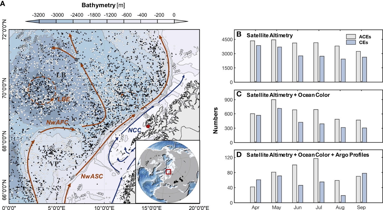
Figure 1 (A) Map of bathymetry and main currents in the northern Norwegian Sea. Locations of snapshots of anticyclonic eddies (ACEs) and snapshots of cyclonic eddies (CEs) detected by available ocean color data for April through September, 2000-2020 are shown by black triangles and white dots. The red dot represents the Lofoten-Vesterålen Islands. Histograms of monthly numbers of (B) all ACEs and CEs identified by satellite altimetry and hybrid algorithm, (C) identified ACEs and CEs based on (B) and covered by ocean color data, and (D) Argo floats occurring within ACEs and CEs based on (C).

2.1.1 Altimetry data

Daily gridded SLA with 0.25 × 0.25° resolution during the past 21 years (2000-2020) were used to identify mesoscale eddies. The gridded Level-4 products from Copernicus Marine Environment Monitoring Services (CMEMS, http://marine.copernicus.eu) were constructed by merging TOPEX/Poseidon, Jason-1/2, ERS-1/2, GFO, CryoSat-2, HY-2A, Altika and ENVISAT mission data. The mesoscale eddies determined by altimetry were collocated to CHL fields at the corresponding temporal and spatial locations based on the center and radius of each eddy to evaluate the CHL response to mesoscale eddies. The automated method used for the detection of mesoscale eddies is described in Section 2.2.

2.1.2 Ocean color

Level-2 CHL and SST products from MODIS Aqua with a spatial resolution of 500 m were obtained from the NASA Ocean Color archive (https://oceancolor.gsfc.nasa.gov) and were used in two case studies (8 June 2017 and 3 July 2019). Level-3 CHL products from Ocean Color Climate Change Initiative (OC-CCI, http://www.oceancolour.org/), derived from merged satellite observations of MERIS, MODIS, OLCI, SeaWiFS, and VIIRS, were used to maximize the available coverage. The OC-CCI product has been validated using a globally compiled in-situ database between 1997 and 2018 (Valente et al., 2019; Ferreira et al., 2022). The in-situ database has more than 2000 observations available for validation in the northern Norwegian Sea. The daily CHL products with a 4 km resolution were used to construct CHL anomalies between April and September between 2000-2020. We use daily CHL observation products, which correspond in time and space to the daily SLA fields, to minimize the loss of data due to cloud cover and poor colocation of weekly or monthly averaged CHL and SLA products.

2.1.3 Wind fields

To study the air-sea interaction over mesoscale eddies, Ekman pumping velocities were estimated from 10-m winds inferred from measurements by the SeaWinds scatterometer on the QuikSCAT and the Advanced scatterometer onboard the ASCAT METOP-A (https://www.remss.com). QuikSCAT covers the period between 19 July 1999 and 23 November 2009, and the ASCAT (Metop-A) data are from 19 October 2006 to 15 November 2021. The combination of these two missions (QuikSCAT for 2000-2009 and ASCAT for 2010-2020) allows coverage over the entire time period. The equivalent neutral vector winds are inferred from the radar backscatter measured by the scatterometers at 10 m relative to the moving sea surface, and are referred to as relative winds (Ross et al., 1985; Chelton and Freilich, 2005; Chelton and Xie, 2010; Gaube et al., 2013).

2.2 Identification of mesoscale eddies

There are several automated eddy detection schemes found in the literature (Jeong and Hussain, 1995; Sadarjoen & Post, 2000; Isern-Fontanet et al., 2006; Chelton et al., 2007; Nencioli et al., 2010; Chelton et al., 2011; Faghmous et al., 2015), of which methods based on the dynamical properties of the flow field and geometric properties are two of the most extensively used (Okubo, 1970; Weiss, 1991; Sadarjoen & Post, 2000; Isern-Fontanet et al., 2006). The method based on dynamical properties of the flow field includes the computation of the Okubo–Weiss parameter, which allows the examination of the relative importance of vorticity of the flow field over the deformation or strain rate flow field below a threshold value. On the other hand, geometric properties of eddies are detected based on the macroscopic synoptic curvature shape of the streamlines of sea-surface height. Halo (2012) showed that by combining the two properties (geometric and dynamical) simultaneously to define an eddy (hybrid method) minimizes considerably the presence of threshold values, hence minimizing subjectivity and produce better results. The performance of the hybrid eddy detection algorithm has been tested successfully in the LB and has been validated using Argo floats and surface drifters (Raj et al., 2015; Raj et al., 2016; Raj and Halo, 2016; Raj et al., 2020).

To identify mesoscale eddies, we use the above-mentioned automatic hybrid eddy detection algorithm that combines the geometric and dynamical properties of the flow field (Halo, 2012; Raj et al., 2015; Raj et al., 2016). The dynamical property is described by the Okubo-Weiss parameter (W) (Okubo, 1970; Weiss, 1991; Harrison & Glatzmaier, 2010; Chelton et al., 2011), which quantifies the relative importance of shearing deformation rate (S_S), stretching deformation rate (S_n) and relative vorticity (ζ) through following relationships:

$\begin{array}{ll}W=(S_s^2+ S_n^2) - {\varsigma }^2& (1)\end{array}$

$\begin{array}{ll}{S}_s=\frac{\partial v\text{'}}{\partial x}+\frac{\partial u\text{'}}{\partial y} & (2)\end{array}$

$\begin{array}{ll} S_n=\frac{\partial u\text{'}}{\partial x}-\frac{\partial v\text{'}}{\partial y} & (3)\end{array}$

$\begin{array}{ll}\varsigma =\frac{\partial v\text{'}}{\partial x}-\frac{\partial u\text{'}}{\partial y} & (4)\end{array}$

where u′ and v′ denote the zonal and meridional components of geostrophic velocity anomalies estimated from SLA using the standard geostrophic relation (Raj et al., 2016). Both shearing (S_s) and stretching (S_n) components are included in Strain (S), S=S_S($S_S^2$+$S_n^2$). W< 0 implies that the vorticity dominates the Strain, which is an essential feature of an eddy. In order to reduce the grid-scale noise two passes of a Hanning filter are applied to W, and regions dominated by vorticity (i.e. negative W) are selected. Note that in order to minimize subjectivity no threshold was imposed on W. The geometric properties of eddies are detected by the closed near-circular contour of SLA field. Corresponding approximately to the altimetry precision shown in Volkov & Pujol (2012), the height interval between the isolines is chosen at ΔSLA = 2 cm. Further, a limit to the equivalent diameters of the closed isolines is set to a maximum of 500 km. Next, by combining the regions of negative W and the regions embedded in closed isolines, the spurious detection associated with noise in W and the ambiguities in multi-poles/elongated closed loops are excluded and thus a more consistent pattern of the eddy is obtained. More details of the algorithm are described in Halo (2012).

The geostrophic eddy kinetic energy (EKE_g) is computed by:

$\begin{array}{ll}EK{E}_g=\frac{u{\text{'}}^2+v{\text{'}}^2}{2} & (5)\end{array}$

while the eddy intensity (EI) is defined as the area-weighted mean EKE_g and A is the surface area (Raj et al., 2015):

$\begin{array}{ll}EI= \frac{1}{A}\underset{A}{\int }EK{E}_g dA& (6)\end{array}$

2.3 Collocation of CHL anomalies with mesoscale eddies

To investigate CHL variability induced by mesoscale eddies, CHL anomalies were constructed to quantify the phytoplankton biomass in ACEs and CEs. Daily maps of CHL were interpolated onto a 0.25°× 0.25° grid to be consistent with the resolution of the SLA fields. The daily 0.25° CHL fields were then spatially high-pass filtered with half-power filter cutoffs of 4° × 4°. The first internal deformation radius, L_d=NH/f, is representative of the horizontal scale of oceanic eddies, where H is vertical extension of the eddy (Yu et al., 2017). The L_d in the northern Norwegian Sea is ~ 15 km, and the 4° × 4° filtering is effective in removing large-scale oceanographic features that are not relevant to the mesoscale variability of interest in this study (not shown; Gaube et al., 2013):

$\begin{array}{ll}Ch{l}_{\text{anom}}=H{P}_{\text{sp}}\left(Chl\right) & (7)\end{array}$

where HP_sp denotes the high-pass filter. The magnitude of the eddy-driven CHL anomalies in northern Norwegian Sea is influenced by location and season. To reduce these effects, the Chl_anom was normalized at longitude x and latitude y by dividing the long-term averaged background fields at the same location:

$\begin{array}{ll}Ch{l}_{\text{norm}}\left(x,y\right)= \frac{Ch{l}_{\text{anom}}\left(x,y\right)}{Ch{l}_{\text{ave}}\left(x,y\right)}& (8)\end{array}$

where Chl_ave(x,y) is the monthly averaged background CHL field over 21 years. The normalized CHL anomalies (Chl_norm) obtained retain seasonal characteristics and are dimensionless and can be considered as partial deviations from the long-term mean. The same process was also performed on SLA and wind stress data.

The average cloud-free coverage of daily OC-CCI dataset within the entire study area (65.5–72°N, 0–20°E) from April to September 2000-2020 is 15.61%. For all eddies identified by satellite altimetry in the study area from April to September 2000-2020, the average cloud-free coverage within one radius of the eddy is 12.01%. Before composites, eddies with more than 70% of the available pixel points in the Chl_norm results within one radius of each known eddy were selected, and eddies with less than 70%-pixel coverage were removed to minimize errors on the composites caused by cloud coverage within the eddy area. The satellite-based estimates of all Chl_norm were then collocated to each snapshots of eddy identified from the SLA fields for normalized composite averages. Total and monthly composite averages of ACEs and CEs from satellite-based Chl_norm results were created to quantify the structure of the CHL response to mesoscale eddy activities. The centers and radius of all eddies are normalized with the radius R. Values of ±1R correspond to the edges of the eddies, while values of zero correspond to the eddy core, thus allowing us to construct composite averages from eddies of different sizes. We extracted data from -2R to 2R to include the interaction between the eddies and the surrounding waters. This method of constructing average eddy composites has been applied to other regions in the global ocean (Chelton et al., 2011; Gaube et al., 2014; Wang et al., 2018; He et al., 2021).

2.4 Eddy-induced Ekman pumping

To investigate the effect of vertical pumping within the eddy on surface CHL anomalies, eddy-induced Ekman pumping velocities were estimated by altimetry-based SLA and scatterometer-derived relative wind fields. Positive (negative) Ekman pumping implies the upward (downward) pumping velocities within the eddy. The surface wind stress (τ) was estimated from QuikSCAT and ASCAT relative equivalent neutral winds using the formula:

$\begin{array}{ll}\tau ={\rho }_{\alpha }{C}_D{u}_{rel}\left|u_{rel}\right| & (9)\end{array}$

where ρ_α is the air density (1.25 kg m^-3) and u_rel is relative wind speed to a surface water mass, which is derived from scatterometry data (Gaube et al., 2013; Gaube et al., 2014; Park et al., 2019). C_D is the speed-dependent drag coefficient, which was determined following Anderson (1993) and Park et al. (2019):

$\begin{array}{ll}{C}_D=7.55\times {10}^{-4},\left|u_{rel}\right|<=4.5{\text{ms}}^{-1}& (10)\end{array}$

$\begin{array}{ll}{C}_D=4\times {10}^{-4}+7.9\times {10}^{-5}\left|u_{rel}\right|,\left|u_{rel}\right|>4.5m{s}^{-1}& (11)\end{array}$

The eddy-induced Ekman pumping was computed as:

$\begin{array}{ll}{W}_E=\frac{\nabla \times \tau }{{\rho }_{0}f} & (12)\end{array}$

where ρ₀=1020 kg m^-3 is the surface density of sea water and f=2Ωcosθ is the Coriolis parameter for latitude θ at an Earth rotation rate of Ω (Gaube et al., 2013). Similar to the processing in Section 2.3, spatial high-pass filtering with half-power filter cutoffs of 4° × 4° and composite average estimation were also performed for Ekman pumping fields for consistency.

2.5 Finite-size Lyapunov exponents (FSLEs)

FSLEs were used as an efficient indicator of the sensitivity of mesoscale eddies to the horizontal exchange of water with ambient waters (Lehahn et al., 2007; He et al., 2017). Daily geostrophic velocity fields from the Level-4 altimetry products were used to calculate FSLE fields by backward LCSs. The FSLEs are computed from the time interval τ, at which two fluid particles move from an initial separation distance δ_i to a final separation distance δ_f following their trajectories in the two-dimensional velocity field. At time t and position x, the Lyapunov exponent λ is defined as:

$\begin{array}{ll}\lambda \left(x, t, {\delta }_i,{\delta }_f\right)=\frac{1}{\tau }\text{log}\left(\frac{{\delta }_f}{{\delta }_i}\right)& (13)\end{array}$

where λ is the local measure of the largest exponential separation rate of two particles (d'Ovidio et al., 2004; d’Ovidio et al., 2009; Dong et al., 2022). The units of FSLEs are d^-1. Trajectories were extracted by applying a fourth-order Runge-Kutta scheme with a time step of 3 h. δ_i and δ_f were set at 0.02° and 0.4° to capture the mesoscale properties and visualize the details of the structures. These structures in the backward FSLE fields are the so-called Lagrangian Coherent Structures (LCSs), which act as transport barriers in the flow field (Lehahn et al., 2011; Dong et al., 2021).

2.6 Mixed layer depths (MLDs)

To further understand how the different types of ACEs and CEs impact mixing and stratification, MLDs were investigated inside and outside of the eddies. We obtained the density-based MLD estimates for all Argo profiles in the northern Norwegian Sea from the global database compiled by Holte & Talley (2009) (http://mixedlayer.ucsd.edu/). Over the 21 years a total of 4,802 Argo profiles were available in the region of 65.5–72° N, 0–20° E (Table 1; Supplementary Figure 1). MLDs derived from the Argo float data were collocated with the SLA-derived eddies based on their locations and corresponding date. An Argo float was determined to be within eddies if it appeared within the outermost closed profile of the SLA used to define the eddy periphery, and otherwise it was outside the eddy as a background field. There were 258 Argo profiles inside ACEs and 217 Argo profiles inside CEs, and were used for MLD analysis (Table 1; Figure 1D, Supplementary Figure 1). The standard error of the mean was used to account for the uncertainty around the estimates of the monthly average MLD and CHL.

TABLE 1

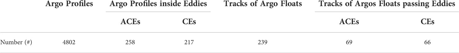
Table 1 Number of Argo Profiles and tracks of Argo Floats between April and September 2000-2020 in the northern Norwegian Sea.

3 Results

3.1 Spatial-temporal distribution characteristics of mesoscale eddies

A total of 24,086 snapshots of ACEs and 18,083 snapshots of CEs, corresponding to 2,671 ACE tracks and 2,489 CE tracks, respectively, were identified from the altimetry data using the hybrid algorithm. Of which 3,841 snapshots of ACEs and snapshots of 2,727 CEs, corresponding to 1,511 ACE tracks and 1,270 CE tracks, respectively, had available ocean color data to be used in this study (Figures 1, 2, Supplementary Figures 2, 3). To investigate the surface CHL response to different types of mesoscale eddies, 1,984 snapshots of ACEs with reduced CHL inside (ACE-), 1,236 snapshots of CEs with elevated CHL inside (CE+), and 1,857 snapshots of ACEs with elevated CHL inside (ACE+), 1,491 snapshots of CEs with reduced CHL inside (CE-) were identified in the northern Norwegian Sea (Figure 2). The western LB (< 3000 m) and the eastern LB near the continental slope off the Lofoten-Vesterålen Islands are important residing areas for both types of ACEs and CEs. Eddies in these two regions occur more frequently and have stronger eddy intensity than in other regions (Figure 2, Supplementary Figures 2-4). The magnitude of eddy intensity of CEs is comparable in the eastern and western of LB, respectively, while the ACEs in the western LB are more intense than the eastern part. 2,757 snapshots of ACEs and 1,755 snapshots of CEs had a lifespan of more than 10 days, 1,710 snapshots of ACEs and 918 snapshots of CEs had a lifespan of more than 20 days, and 631 snapshots of ACEs and 158 snapshots of CEs had a lifespan of more than 60 days (Tables 2, Supplementary Figure 3). The longer-lived eddies occurred in the western LB and areas near the continental slope (Supplementary Figure 3). In addition, ACEs in the western LB were centered at 3°E, 69.8°N in a circular pattern, coinciding with the location of the LBE; CEs in the western LB are also mainly distributed in the deepest part of the basin. ACEs in the eastern LB are distributed along the continental slope, while the center of distribution for CEs is 12°E, 69.5°N.

FIGURE 2

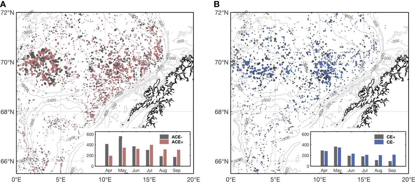
Figure 2 Location of identified (A) 3,841 snapshots of ACEs and (B) 2,727 snapshots of CEs covered by available ocean color data in the northern Norwegian Sea during April to September 2000-2020. (A) The gray and red dots represent ACEs with reduced CHL inside (ACE-) and ACEs with elevated CHL inside (ACE+), respectively, and (B) the gray and blue dots represent CEs with elevated CHL inside (CE+) and CEs with reduced CHL inside (CE-). The size of dots represents the relative magnitude of EI. Monthly numbers of the ACE-, ACE+, CE+, and CE- are shown in the insets.

TABLE 2

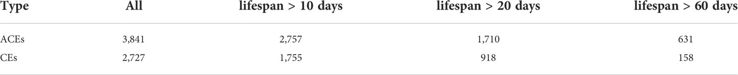
Table 2 Number of identified ACEs and CEs with different lifespans covered by available Ocean Color data.

3.2 Revealing CHL anomalies associated with mesoscale eddies from case studies

Two cases (on 3 July 2019 and 8 June 2017) illustrate that mesoscale eddies can considerably affect the distribution of surface CHL in the northern Norwegian Sea (Figures 3, 4). CE+ elevated CHL within the eddy by two orders of magnitude relative to the surrounding waters on 3 July 2019 (Figure 3). ACE- with elevated SLA decreased the CHL within the eddy relative to the surrounding waters on 8 July 2017 (Figure 4). A large number of eddies also exhibited the unusual opposite pattern, with elevated CHL within ACEs and lower CHL within CEs (ACE+ and CE- in Figures 3 and 4). For example, one of the ACE+ located in the region of 70.2–71.2° N, 6.5–10.5° E on 3 July 2019 showed greater CHL and lower SST (Figure 3). Similar patterns are also observed on 8 June 2017 with a pair of dipole eddies in 69–70.2° N, 1–5° E, where a greater CHL within the ACE+ and a lower CHL within the CE- (Figure 4). The extremes of the LCS curves for each eddy correspond to the edge of the eddy with the greatest geostrophic current velocity that separates the water within the eddy from the surrounding waters (Figures 3B, D and 4B, D). The water particles on both sides move along the LCSs, which act as transport barriers limiting the horizontal exchange of water between the two sides, resulting in large differences in CHL and SST field inside and outside the eddies. This effect retains water with larger/smaller CHL inside eddies.

FIGURE 3

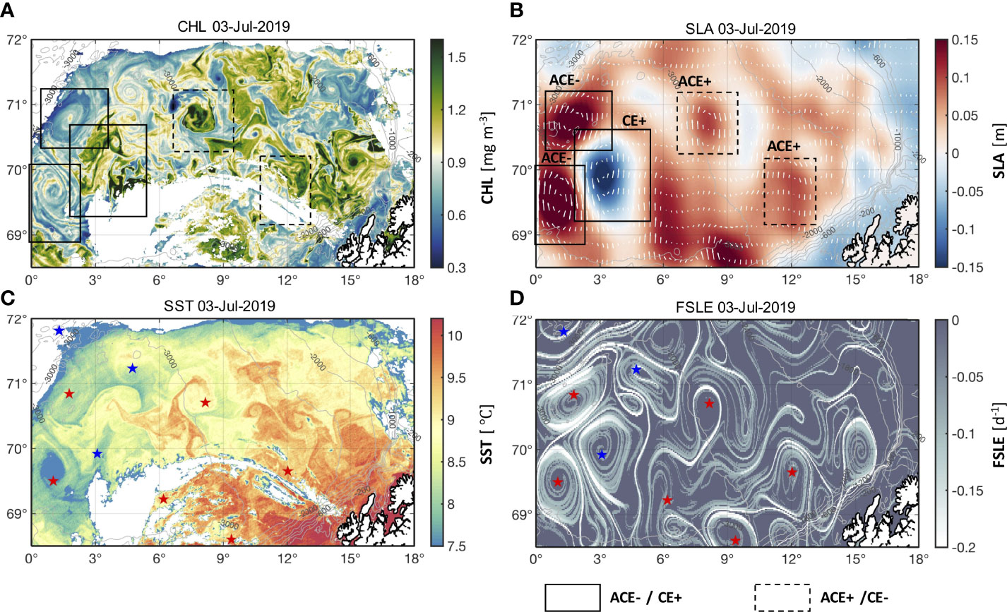
Figure 3 Spatial distribution of (A) CHL, (B) SLA, (C) sea surface temperature (SST), and (D) Finite-size Lyapunov Exponent (FSLE) for 3 July 2019. ACE- and CE+ in (A, B) are demarcated by solid boxes; ACE+ and CE- in (A, B) are demarcated by dashed boxes. ACEs and CEs in (C, D) are indicated by red and blue stars, respectively.

FIGURE 4

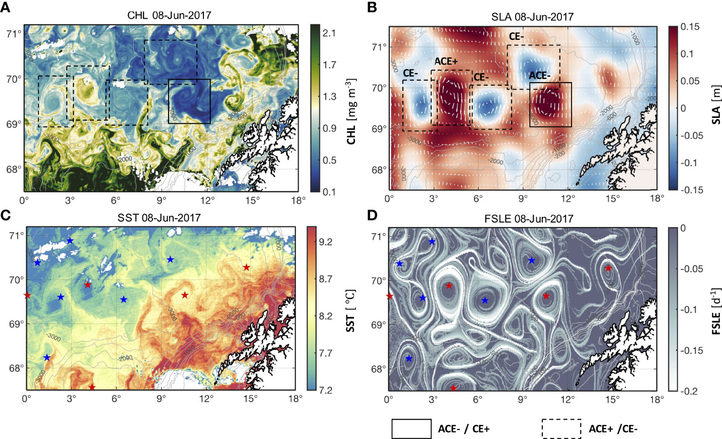
Figure 4 Spatial distribution of (A) CHL, (B) SLA, (C) sea surface temperature (SST), and (D) Finite-size Lyapunov Exponent (FSLE) for 8 June 2017. ACE- and CE+ in (A, B) are demarcated by solid boxes; ACE+ and CE- in (A, B) are demarcated by dashed boxes. ACEs and CEs in (C, D) are indicated by red and blue stars.

3.3 Eddy induced Ekman pumping causing unusual CHL anomalies within eddies

To investigate the response mechanism of the unusual surface CHL anomalies to mesoscale eddies, composite averages of the CHL anomalies, SLA and eddy-induced Ekman pumping were constructed. It appeared that elevated SLA (solid contours in Figure 5A) lead to downwelling, resulting in negative CHL anomalies within ACE-, while reduced SLA (dashed contours in Figure 5B) lead to upwelling, resulting in positive CHL anomalies within CE+. Averaged structure and monthly evolution of the composite CHL anomalies of ACEs and CEs show that eddy-induced Ekman pumping was strongly correlated with the unusual CHL enhancements (decreases) in the ACEs (CEs) (Figures 5C, D and 6). Eddy-induced Ekman pumping is generated by sea surface stress curl resulting from surface differential currents associated with mesoscale eddies and wind fields. The polarity of this surface stress curl is opposite to the vorticity of the eddy; hence, the net result is Ekman upwelling within ACEs (solid contours in Figures 5C and 6A–F) and Ekman downwelling within CEs (dashed contours in Figures 6D, G–L). This process is largely responsible for the unusual positive (negative) CHL anomalies at the interior of the ACEs (CEs) (Figures 5C, D, and 6). In particular, our analysis shows that the signal of CHL anomalies within ACE+ is much stronger than that within ACE-, CE+ and CE-, with CHL anomalies over 0.2 mg m^-3 appearing close to ±0.5R (Figure 5). The maximum eddy-induced Ekman pumping rate for ACE+ occurred in April and May, whereas the monthly composite averages of CHL anomalies for ACE+ in May and June were more than twice as large as those in April (Figures 6A–C). The signal of CHL anomalies was also stronger in May and June for CE- than in April, but the differences were not considerable (Figures 6G–I, Supplementary Table 1).

FIGURE 5

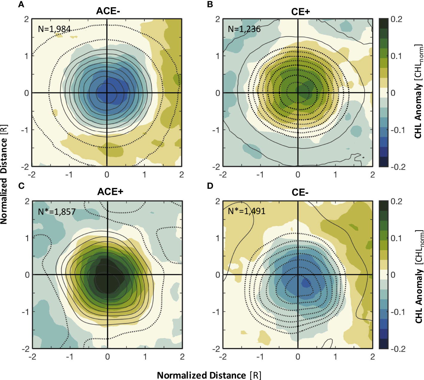
Figure 5 Total composite averages of CHL anomalies for (A) ACE-, (B) CE+, (C) ACE+, and (D) CE- in the northern Norwegian Sea for April to September. The contours in (A, B) represent the composite averages of SLA (contour interval 1 cm), and those in (C, D) represent eddy-induced Ekman pumping (contour interval 1 cm d^-1). Positive SLA and Ekman pumping are represented as solid curves; negative SLA and Ekman pumping are represented as dashed curves. The x and y coordinates of the composite averages are normalized by the eddy radius (R). N and N* represent the number of eddy realizations for construction of the composites.

FIGURE 6

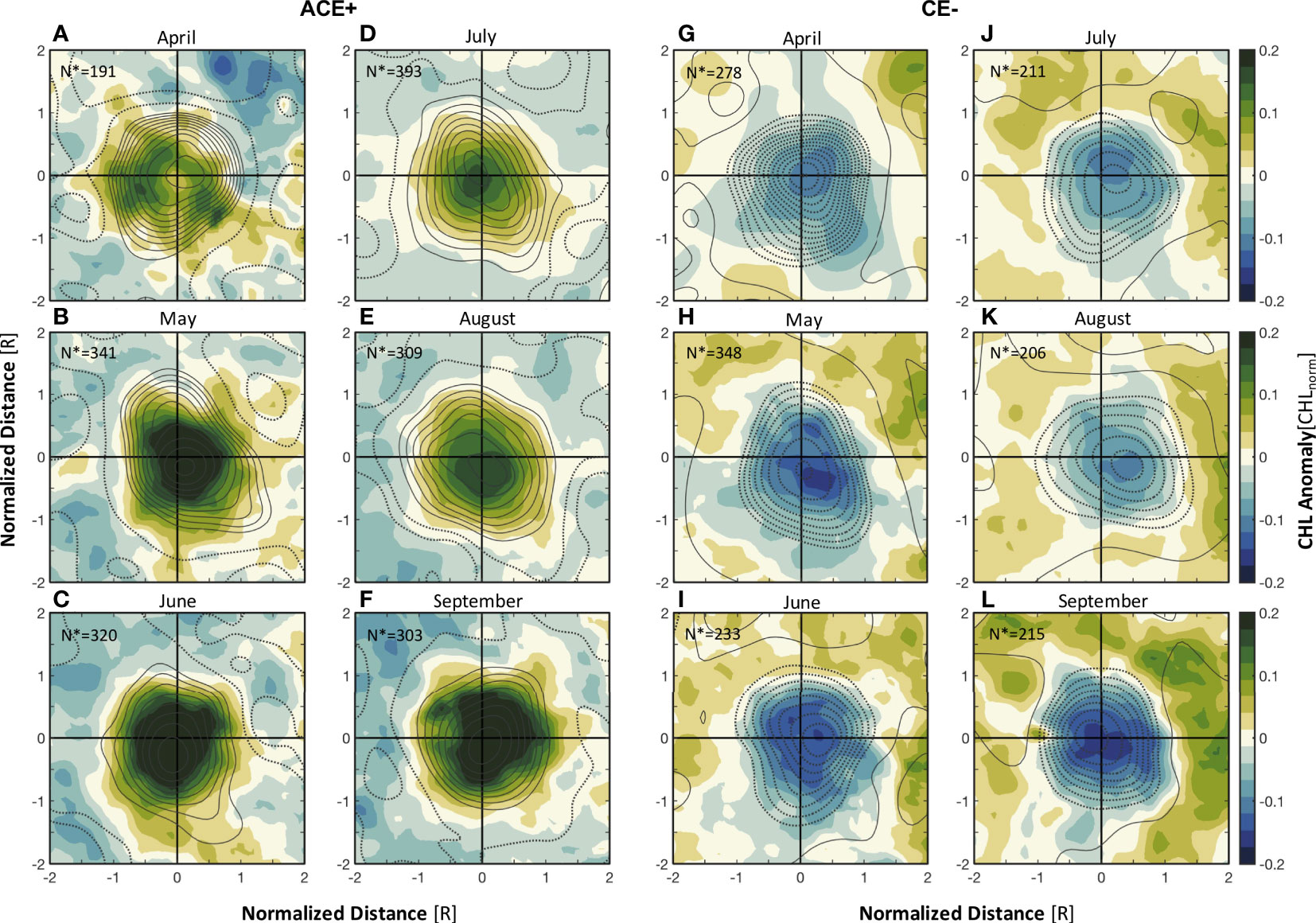
Figure 6 Monthly composites (April-September) of CHL anomalies for (A–F) ACE+ and (G–L) CE- in the northern Norwegian Sea for 2000-2020. The contours in (A–L) represent the composites of eddy-induced Ekman pumping (contour interval 1 cm d^-1); solid lines correspond to upward pumping velocities, dashed lines correspond to downward pumping velocities. The x and y coordinates are normalized by the eddy radius (R). N* represents the number of eddy realizations for construction of the composite.

3.4 MLD variations associated with mesoscale eddies

To further assess whether the CHL anomalies within the different types of mesoscale eddies and their associated Ekman pumping affect the processes occurring below the surface, we investigated the monthly variations of MLD within the ACE-, ACE+, CE+, CE-, and those outside the eddies (Figures 7A, B). For all months, the ACE+ reduced the MLD compared to ACE-, while CE- deepened the MLD (Figures 7A, B). This was caused by the eddy-induced Ekman pumping upward (downward) displacing isopycnals within the ACEs (CEs). This process results in nutrients being introduced into the surface layer from below within the ACE+, so that the increased phytoplankton biomass results in greater CHL in the core of the ACE+ compared to that of the ACE-. Similarly, CHL in the core of CE- has lower CHL in all months compared to CE+ (Figures 7C, D).

FIGURE 7

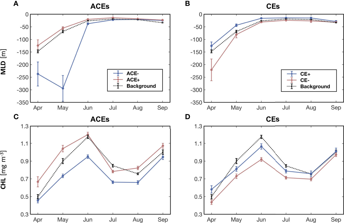
Figure 7 Monthly (A) MLD and (C) CHL for ACE- (blue lines) and ACE+ (red lines); monthly (B) MLD and (D) CHL for CE+ (blue lines) and CE- (red lines); background values (dashed black lines) outside eddies. Standard errors within each month are shown as vertical bars. The differences in MLD between (A) ACE+ and ACE-, (B) CE+ and CE- are significantly at the 95% confidence level. The differences in CHL between (C) ACE+ and ACE-, (D) CE+ and CE- are significantly at the 95% confidence level.

The increase in background CHL from April to June is strongly associated with the seasonal shoaling of the MLD (ΔMLD>100m), which increase the mean irradiance within the mixed layer and stimulates phytoplankton growth. The shoaling of the MLD is also associated with an increase in seasonal heat input into the surface layer. As a result, the background CHL outside eddies also increases from April to June (Figures 7C, D). The presence of ACE+ and CE- caused by eddy-wind interactions further play a role in the vertical mixing of nutrients and CHL within the eddies, so that the CHL anomalies in the eddies peak in May and June (Figure 6). After June, the shallow MLD restricts the vertical input of nutrients into the upper layers, ultimately leading to a decrease in CHL (Figure 7).

4 Discussion

4.1 Radius and lifespan scales of the eddies in the northern Norwegian Sea

The dominant radius scales of the 6568 snapshots of eddies in the northern Norwegian Sea range from 20 to 65 km. More than 2/3 of eddies have radii greater than 30 km and lifespans greater than 10 days (Tables 2, 3). The small radius and lifespan scales of the mesoscale eddies in the study area correspond to the small local Rossby deformation radius (~ 15 km) in this high latitude region. Previous studies have reported that latitudinal dependence is responsible for the smaller radius and lifespan scales of mesoscale eddies in high latitudes than in low and middle latitude regions (Chelton et al., 2011; Chen and Han, 2019). The relatively longer-lived eddies occur in the western LB and areas near the continental slope and are dominated by ACEs (Supplementary Figure 3). In particular, the location of the longer-lived ACEs in western LB coincides with the residence of the LBE, suggesting that the long lifespan of the ACEs may be related to the maintenance mechanism of the eddy mergers in this region (Raj et al., 2015; Raj et al., 2016).

TABLE 3

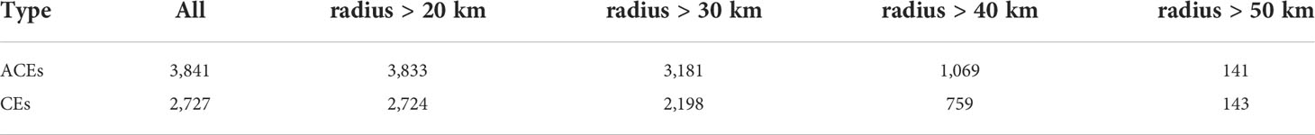
Table 3 Number of identified ACEs and CEs of different radii covered by available Ocean Color data.

4.2 Do ACEs have greater phytoplankton biomass than CEs?

Our study reveals that ACE+ associated with eddy-induced Ekman pumping plays an important role in elevated phytoplankton biomass in the northern Norwegian Sea. This effect can only be ascertained by separating the ACE+ triggered by eddy-induced Ekman upwelling from ACE-, CE+, and CE- (Figure 5). Downwelling caused by the elevated SLA within ACE- suppresses the increase of phytoplankton biomass in the northern Norwegian Sea. The greatest positive CHL anomalies for ACE+ and the lowest negative anomalies for ACE- occurred in May and June, implying that wind-eddy interactions play an important role in the shift of ACE phytoplankton biomass polarity (Figures 5, 6, Supplementary Table 1). The upwelling caused by the reduced SLA within CE+ also raises the CHL within the eddy, but the positive CHL anomalies within CE+ are much weaker than those within ACE+ (Figure 5). This may be related to the deeper MLD in the LB, which allowed the longer-lived ACE-dominated eddies (Supplementary Figure 3) to have more nutrients; in spring, increased seasonal light, shoaling of MLD in the LB, and eddy-induced Ekman upwelling combine to promote phytoplankton growth and further elevated CHL within the ACE+ (Lévy et al., 1998; Mahadevan et al., 2012; He et al., 2017). In May and June, the seasonal shoaling of the MLD led to greater irradiance levels available for phytoplankton growth, stimulating phytoplankton growth and accumulation in the surface layer of the ACE+ (Figure 7). This seasonal wind-eddy-biological interaction generates conditions within ACEs that results in ACEs being productive mesoscale features and being more productive than CEs in the northern Norwegian Sea.

4.3 Effects of eddy trapping and stirring processes

Spring phytoplankton blooms in the northern Norwegian Sea occur initially on the continental shelf for several weeks and then move off-shelf from late April (Bagøien et al., 2012). Mesoscale eddies play an important role in this cross-slope transport process and move nutrients and plankton from the shelf to deep water (Dong et al., 2021). Our analysis reveals that ACEs in eastern LB are mainly distributed along the continental slope, while CEs are not (Figure 2). This implies that ACEs may be more commonly shed from the NwASC than CEs and play a more important role in transporting nutrients and plankton from the continental shelf to the open sea. Eddy stirring occurs primarily at the eddy peripheries, resulting in dipoles of positive and negative CHL signals depending on the strength and direction of the background CHL gradient and the intensity of the eddies (Travis & Qiu, 2020). These two mechanisms redistribute CHL spatially through horizontal advection and do not affect the changes in phytoplankton biomass associated with vertical pumping and mixing in mesoscale eddies, and thus are not addressed in these study.

4.4 Other vertical pumping mechanisms

Other vertical pumping processes associated with mesoscale eddies include mode-water eddies and submesoscale pumping in eddies. Mode-water eddies are characterized by a lens-shaped water mass within the core that raises the seasonal pycnocline in the surface layer and depresses the main pycnocline below the lens. Previous studies have shown that the mode-water eddies are dominated by downward displacing of main pycnoclines, and have positive SLA, which makes it impossible to distinguish them from regular ACEs by satellite altimetry (McGillicuddy et al., 2007). Due to the elevated productivity and positive SLA of the mode-water eddies, we consider any potential mode-water eddies in the northern Norwegian Sea to be included in ACE+.

At the periphery of the eddy, front-like features can develop at the velocity maximum (corresponding to FSLE extremes of each eddy; Figures 3D and 4D), with submesoscale upwelling and downwelling generated along the eddy front, and where vertical pumping velocities can reach 10 m d^-1 (Siegel et al., 2011). This potential submesoscale pumping can greatly increase the nutrient flux and phytoplankton growth around the eddy, but the horizontal scale is not large enough to obtain their composite average results from ocean color and altimetry products. While submesoscale productivity may be important, it cannot be adequately resolved by our methods.

4.5 Potential impacts on higher trophic levels

The dominant copepod in the Norwegian Sea is C. finmarchicus, which serves as a key link between primary producers and higher trophic levels (Planque, 2000; Melle et al., 2014). The spatio-temporal distribution of C. finmarchicus appears to be strongly correlated with CHL (Supplementary Figure 5). As a result, understanding CHL anomalies in different types of mesoscale eddies is not only important for phytoplankton biomass, but also can affect the spatial distribution of zooplankton and higher trophic levels (Melle et al., 2014; Basedow et al., 2019). Other zooplankton are known to have increased biomass and activity in mesoscale and submesoscale “hotspots” (Basedow et al., 2019; Weidberg et al., 2022), and it is likely that the important grazers of the Norwegian system likewise utilize eddies, and particularly the ACE+ with elevated phytoplankton biomass, as important regions in their life cycles.

5 Conclusions

This study reveals unusual surface CHL anomalies caused by mesoscale eddies, manifested as positive CHL anomalies within ACEs and negative CHL anomalies within CEs, and that these CHL anomalies are triggered by Ekman pumping due to wind-eddy interactions. Given their ubiquitous distribution, these eddies play an important role in biogeochemical processes in the northern Norwegian Sea. The composite results of the CHL and wind anomalies indicate that the eddy-induced Ekman upwelling within ACEs cause stronger CHL anomalies than other types of eddies, which is responsible for the large phytoplankton biomass within ACEs in the region.

The CHL anomaly maxima induced by Ekman pumping mechanisms occur in May and June, which are the months associated with the spring blooms in the northern Norwegian Sea. Further analysis of the MLD indicated that from April to June, the MLD were reduced, resulting a greater irradiance environment for phytoplankton growth. After June, the shallow MLD prevented the vertical input of nutrients into the upper ocean. The combined physical-biological processes play a critical role in generating surface CHL anomalies and is a major factor in the regulation of phytoplankton biomass in the northern Norwegian Sea.

Data availability statement

The original contributions presented in the study are included in the article/Supplementary Material. Further inquiries can be directed to the corresponding authors.

Author contributions

HD and MZ designed the original ideas. HD and RR performed the data processing and analyses. WS, RJ, and CA contribute to the concept of the manuscript. HD wrote the original manuscript, WS, RR, ZZ, SB, and MZ revised and improved the manuscript. All authors contributed to the article and approved the submitted version.

Acknowledgments

This work is supported by the Sino-Norway Collaborative STRESSOR Project, funded by the Natural Science Foundation of China (NSFC Grant No. 41861134040) and the Research Council of Norway (RCN Grant No.287043). This study is also supported by the NSFC Special Program (Grant No. 41941008) and Shanghai Frontiers Science Center of Polar Science (SCOPS). Author Raj is supported by the European Space Agency (Prodex project S23Deddy, Contract No. 4000135226) and the Bjerknes Fast Track Initiative project Qrepe. The authors have no conflicts of interest with these data. We thank Huijie Xue, Zhongping Lee for valuable comments. We also thank Shengyang Fang for valuable comments and language revisions.

Conflict of interest

The authors declare that the research was conducted in the absence of any commercial or financial relationships that could be construed as a potential conflict of interest.

Publisher’s note

All claims expressed in this article are solely those of the authors and do not necessarily represent those of their affiliated organizations, or those of the publisher, the editors and the reviewers. Any product that may be evaluated in this article, or claim that may be made by its manufacturer, is not guaranteed or endorsed by the publisher.

Supplementary material

The Supplementary Material for this article can be found online at: https://www.frontiersin.org/articles/10.3389/fmars.2022.1002632/full#supplementary-material

References

Abraham E. R. (1998). The generation of plankton patchiness by turbulent stirring. Nature 391, 577–580. doi: 10.1038/35361

CrossRef Full Text | Google Scholar

Anderson R. J. (1993). A study of wind stress and heat flux over the open ocean by the inertial-dissipation method. J. Phys. Oceanogr. 23, 2153–2161. doi: 10.1175/1520-0485(1993)023<2153:ASOWSA>2.0.CO;2

CrossRef Full Text | Google Scholar

Bagøien E., Melle W., Kaartvedt S. (2012). Seasonal development of mixed layer depths, nutrients, chlorophyll and Calanus finmarchicus in the Norwegian Sea – a basin-scale habitat comparison. Prog. Oceanogr. 103, 58–79. doi: 10.1016/J.POCEAN.2012.04.014

CrossRef Full Text | Google Scholar

Basedow S. L., McKee D., Lefering I., Gislason A., Daase M., Trudnowska E., et al. (2019). Remote sensing of zooplankton swarms. Sci. Rep. 9, 686. doi: 10.1038/S41598-018-37129-X

PubMed Abstract | CrossRef Full Text | Google Scholar

Chapman C. C., Lea M.-A., Meyer A., Salee J.-B., Hindell M. (2020). Defining southern ocean fronts and their influence on biological and physical processes in a changing climate. Nat. Climate Change 10, 209–219. doi: 10.1038/S41558-020-0705-4

CrossRef Full Text | Google Scholar

Chelton D., Freilich M. (2005). Scatterometer-based assessment of 10-m wind analyses from the operational ECMWF and NCEP numerical weather prediction models. Monthly Weather Rev. 133, 409–429. doi: 10.1175/MWR-2861.1

CrossRef Full Text | Google Scholar

Chelton D. B., Schlax M. G., Samelson R. M. (2011). Global observations of nonlinear mesoscale eddies. Prog. Oceanogr. 91, 167–216. doi: 10.1016/J.POCEAN.2011.01.002

CrossRef Full Text | Google Scholar

Chelton D. B., Schlax M. G., Samelson R. M., Szoeke R. A. (2007). Global observations of large oceanic eddies. Geophys. Res. Lett. 34, L15606. doi: 10.1029/2007GL030812

CrossRef Full Text | Google Scholar

Chelton D., Xie S. (2010). Coupled ocean-atmosphere interaction at oceanic mesoscales. Oceanography 23, 52–69. doi: 10.5670/oceanog.2010.05

CrossRef Full Text | Google Scholar

Chen G., Han G. (2019). Contrasting short-lived with long-lived mesoscale eddies in the global ocean. J. Geophys. Res.: Oceans 124, 3149–3167. doi: 10.1029/2019JC014983

CrossRef Full Text | Google Scholar

d'Ovidio F., Fernández V., Hernández-García E., López C. (2004). Mixing structures in the Mediterranean Sea from finite-size lyapunov exponents. Geophys. Res. Lett. 31, L17203. doi: 10.1029/2004GL020328

CrossRef Full Text | Google Scholar

Dawson H. R. S., Strutton P. G., Gaube P. (2018). The unusual surface chlorophyll signatures of southern ocean eddies. J. Geophys. Res.: Oceans 123, 6053–6069. doi: 10.1029/2017JC013628

CrossRef Full Text | Google Scholar

Dong H., Zhou M., Hu Z., Zhang Z., Zhong Y., Basedow S. L., et al. (2021). Transport barriers and the retention of Calanus finmarchicus on the lofoten shelf in early spring. J. Geophys. Res.: Oceans 126, e2021JC017408. doi: 10.1029/2021JC017408

CrossRef Full Text | Google Scholar

Dong H., Zhou M., Smith W. O., Li B., Hu Z., Basedow S. L., et al. (2022). Dynamical controls of the Eastward transport of overwintering Calanus finmarchicus from the lofoten basin to the continental slope. J. Geophys. Res.: Oceans 127, e2022JC018909. doi: 10.1029/2022JC018909

CrossRef Full Text | Google Scholar

d’Ovidio F., Isern-Fontanet J., Lopez C., Hernandez-Garcia E., Garcia-Ladona E. (2009). Comparison between eulerian diagnostics and finite-size lyapunov exponents computed from altimetry in the Algerian basin. Deep Sea Res. I 56, 15–31. doi: 10.1016/J.DSR.2008.07.014

CrossRef Full Text | Google Scholar

Dufois F., Hardman-Mountford N. J., Greenwood J., Richardson A. J., Feng M., Matear R. (2016). Anticyclonic eddies are more productive than cyclonic eddies in subtropical gyres because of winter mixing. Sci. Adv. 2, e1600282. doi: 10.1126/SCIADV.1600282

PubMed Abstract | CrossRef Full Text | Google Scholar

Faghmous J. H., Frenger I., Yao Y., Warmka R., Lindell A., Kumar V. (2015). A daily global mesoscale ocean eddy dataset from satellite altimetry. Sci. Data 2, 150028. doi: 10.1038/SDATA.2015.28

PubMed Abstract | CrossRef Full Text | Google Scholar

Fer I., Bosse A., Dugstad J. (2020). Norwegian Atlantic Slope current along the lofoten escarpment. Ocean Sci. 16, 685–701. doi: 10.5194/OS-16-685-2020

CrossRef Full Text | Google Scholar

Ferreira A., Dias J., Brotas V., Brito A. C. (2022). A perfect storm: An anomalous offshore phytoplankton bloom event in the NE Atlantic (March 2009). Sci. Total Environ. 806, 151253. doi: 10.1016/J.SCITOTENV.2021.151253

PubMed Abstract | CrossRef Full Text | Google Scholar

Frenger I., Münnich M., Gruber N. (2018). Imprint of southern ocean mesoscale eddies on chlorophyll. Biogeosciences 15, 4781–4798. doi: 10.5194/BG-15-4781-2018

CrossRef Full Text | Google Scholar

Gaube P., Chelton D. B., Strutton P. G., Behrenfeld M. J. (2013). Satellite observations of chlorophyll, phytoplankton biomass, and ekman pumping in nonlinear mesoscale eddies. J. Geophys. Res.: Oceans 118, 6349–6370. doi: 10.1002/2013JC009027

CrossRef Full Text | Google Scholar

Gaube P., McGillicuddy D. J. Jr., Chelton D. B., Behrenfeld M. J., Strutton P. G. (2014). Regional variations in the influence of mesoscale eddies on near-surface chlorophyll. J. Geophys. Res.: Oceans 119, 8195–8220. doi: 10.1002/2014JC010111

CrossRef Full Text | Google Scholar

Guo M., Xiu P., Li S., Chai F., Xue H., Zhou K., et al. (2017). Seasonal variability and mechanisms regulating chlorophyll distribution in mesoscale eddies in the south China Sea. J. Geophys. Res.: Oceans 122, 5329–5347. doi: 10.1002/2016JC012670

CrossRef Full Text | Google Scholar

Halo I. (2012). “The Mozambique channel eddies: Characteristics and mechanisms of formation,” in PhD Thesis (Cape Town, South Africa: University of Cape Town).

Google Scholar

Hansen C., Kvaleberg E., Samuelsen A. (2010). Anticyclonic eddies in the Norwegian Sea: Their generation, evolution and impact on primary production. Deep Sea Res. I 57, 1079–1091. doi: 10.1016/J.DSR.2010.05.013

CrossRef Full Text | Google Scholar

Harrison C. S., Glatzmaier G. A. (2010). Lagrangian Coherent structures in the California current system–sensitivities and limitations. Geophys. Astrophysical Fluid Dynamics 106, 22–44. doi: 10.1080/03091929.2010.532793

CrossRef Full Text | Google Scholar

Helland-Hansen B., Nansen F. (1909). The Norwegian Sea: Its physical oceanography based upon the Norwegian research 1900–1904. Rep. Norwegian Fishery Mar. Invest. 2, 1–360.

Google Scholar

He Q., Zhan H., Cai S., Zhan W. (2021). Eddy-induced near-surface chlorophyll anomalies in the subtropical gyres: Biomass or physiology? Geophys. Res. Lett. 48, e2020GL091975. doi: 10.1029/2020GL091975

CrossRef Full Text | Google Scholar

He Q., Zhan H., Shuai Y., Cai S., Li Q. P., Huang G., et al. (2017). Phytoplankton bloom triggered by an anticyclonic eddy: The combined effect of eddy-ekman pumping and winter mixing. J. Geophys. Res.: Oceans 122, 4886–4901. doi: 10.1002/2017JC012763

CrossRef Full Text | Google Scholar

He Q., Zhan H., Xu J., Cai S., Zhan W., Zhou L., et al. (2019). Eddy-induced chlorophyll anomalies in the western south China Sea. J. Geophys. Res.: Oceans 124, 9487–9506. doi: 10.1029/2019JC015371

CrossRef Full Text | Google Scholar

Holte J., Talley L. (2009). A new algorithm for finding mixed layer depths with applications to argo data and subantarctic mode water formation. J. Atmospheric Oceanic Technol. 26, 1920–1939. doi: 10.1175/2009JTECHO543.1

CrossRef Full Text | Google Scholar

Isachsen P. E. (2015). Baroclinic instability and the mesoscale eddy field around the lofoten basin. J. Geophys. Res.: Oceans 120, 2884–2903. doi: 10.1002/2014JC010448

CrossRef Full Text | Google Scholar

Isern-Fontanet J., Garcia-Ladona E., Font J. (2006). Vortices of the Mediterranean Sea: An altimetric perspective. J. Phys. Oceanogr. 36, 87–103. doi: 10.1175/JPO2826.1

CrossRef Full Text | Google Scholar

Jeong J., Hussain F. (1995). On the identification of a vortex. J. Fluid Mechanics 285, 69–94. doi: 10.1017/S0022112095000462

CrossRef Full Text | Google Scholar

Lehahn Y., d’Ovidio F., Lévy M., Amitai Y., Heifetz E. (2011). Long range transport of a quasi-isolated chlorophyll patch by an agulhas ring. Geophys. Res. Lett. 38, L16610. doi: 10.1029/2011GL048588

CrossRef Full Text | Google Scholar

Lehahn Y., d’Ovidio F., Lévy M., Heifetz E. (2007). Stirring of the northeast Atlantic spring bloom: A Lagrangian analysis based on multisatellite data. J. Geophys. Res. 112, C08005. doi: 10.1029/2006JC003927

CrossRef Full Text | Google Scholar

Lévy M., Mémery L., Madec G. (1998). The onset of a bloom after deep winter convection in the northwestern Mediterranean Sea: Mesoscale process study with a primitive equation model. J. Mar. Syst. 16, 7–21. doi: 10.1016/S0924-7963(97)00097-3

CrossRef Full Text | Google Scholar

Mahadevan A., D'Asaro E., Lee C., Perry M. J. (2012). Eddy-driven stratification initiates north Atlantic spring phytoplankton blooms. Science 337, 54–58. doi: 10.1126/SCIENCE.1218740

PubMed Abstract | CrossRef Full Text | Google Scholar

McGillicuddy D. J. Jr. (2016). Mechanisms of physical-biological-biogeochemical interaction at the oceanic mesoscale. Annu. Rev. Mar. Sci. 8, 125–159. doi: 10.1146/ANNUREV-MARINE-010814-015606

CrossRef Full Text | Google Scholar

McGillicuddy D. J. Jr, Anderson L. A., Bates N. R., Bibby T., Buesseler K. O., et al. (2007). Eddy/wind interactions stimulate extraordinary mid-ocean plankton blooms. Science 316, 1021–1026. doi: 10.1126/SCIENCE.1136256

PubMed Abstract | CrossRef Full Text | Google Scholar

McWilliams J., Flierl G. (1979). On the evolution of isolated, nonlinear vortices. J. Phys. Oceanogr. 9, 1155–1182. doi: 10.1175/1520-0485(1979)009<1155:OTEOIN>2.0.CO;2

CrossRef Full Text | Google Scholar

Melle W., Runge J., Head E., Plourde S., Castellani C., Licandro P., et al. (2014). The north Atlantic ocean as habitat for Calanus finmarchicus: Environmental factors and life history traits. Prog. Oceanogr. 129, 244–284. doi: 10.1016/J.POCEAN.2014.04.026

CrossRef Full Text | Google Scholar

Nencioli F., Dong C., Dickey T., Washburn L., McWilliams J. C. (2010). A vector geometry-based eddy detection algorithm and its application to a high-resolution numerical model product and high-frequency radar surface velocities in the southern California bight. J. Atmospheric Oceanic Technol. 27, 564–579. doi: 10.1175/2009JTECHO725.1

CrossRef Full Text | Google Scholar

Nurser A. J. G., Bacon S. (2014). The rossby radius in the Arctic ocean. Ocean Sci. 10, 967–975. doi: 10.5194/OS-10-967-2014

CrossRef Full Text | Google Scholar

Okubo A. (1970). Horizontal dispersion of floatable particles in the vicinity of velocity singularities such as convergences. Deep Sea Res. Oceanogr. Abstract 17, 445–454. doi: 10.1016/0011-7471(70)90059-8

CrossRef Full Text | Google Scholar

Omand M. M., D’Asaro E. A., Lee C. M., Perry M. J., Briggs N., Cetinic I., et al. (2015). Eddy-driven subduction exports particulate organic carbon from the spring bloom. Science 348, 222–225. doi: 10.1126/SCIENCE.1260062

PubMed Abstract | CrossRef Full Text | Google Scholar

Park J.-E., Park K.-A., Kang C.-K., Park Y.-J. (2019). Short-term response of chlorophyll-a concentration to change in sea surface wind field over mesoscale eddy. Estuaries Coasts 43, 646–660. doi: 10.1007/S12237-019-00643-W

CrossRef Full Text | Google Scholar

Planque B. (2000). Calanus finmarchicus in the north Atlantic: The year of Calanus in the context of interdecadal change. ICES J. Mar. Sci. 57, 1528–1535. doi: 10.1006/JMSC.2000.0970

CrossRef Full Text | Google Scholar

Raj R. P., Chafik L., Nilsen J., Eldevik T., Halo I. (2015). The lofoten vortex of the Nordic seas. Deep Sea Res. I 96, 1–14. doi: 10.1016/J.DSR.2014.10.011

CrossRef Full Text | Google Scholar

Raj R. P., Halo I. (2016). Monitoring the mesoscale eddies of the lofoten basin: Importance, progress, and challenges. Int. J. Remote Sens. 37, 3712–3728. doi: 10.1080/01431161.2016.1201234

CrossRef Full Text | Google Scholar

Raj R. P., Halo I., Chatterjee S., Belonenko T., Bakhoday-Paskyabi M., Bashmachnikov I., et al. (2020). Interaction between mesoscale eddies and the gyre circulation in the lofoten basin. J. Geophys. Res.: Oceans 125, e2020JC016102. doi: 10.1029/2020JC016102

CrossRef Full Text | Google Scholar

Raj R. P., Johannessen J. A., Eldevik T., Nilsen J. E. Ø., Halo I. (2016). Quantifying mesoscale eddies in the lofoten basin. J. Geophys. Res.: Oceans 121, 4503–4521. doi: 10.1002/2016JC011637

CrossRef Full Text | Google Scholar

Richards G. C., Straneo F. (2015). Observations of water mass transformation and eddies in the lofoten basin of the Nordic seas. J. Phys. Oceanogr. 45, 1735–1756. doi: 10.1175/JPO-D-14-0238.1

CrossRef Full Text | Google Scholar

Ross D., Overland J., Plerson W., Cardone V., McPherson R., Yu T. (1985). Oceanic surface winds. Adv. Geophys. 27, 101–140. doi: 10.1016/S0065-2687(08)60404-5

CrossRef Full Text | Google Scholar

Sadarjoen I., Post F. H. (2000). Detection, quantification, and tracking of vortices using streamline geometry. Comput. Graphics 24, 333–341. doi: 10.1016/s0097-8493(00)00029-7

CrossRef Full Text | Google Scholar

Sætre R. (1999). Features of the central Norwegian shelf circulation. Continental Shelf Res. 19, 1809–1831. doi: 10.1016/S0278-4343(99)00041-2

CrossRef Full Text | Google Scholar

Siegel D., Court D., Menzies D., Peterson P., Maritoena S., Nelson N. (2007). Satellite and in situ observation of the bio-optical signatures of two mesoscale eddies in the Sargasso Sea. Deep Sea Res. II 55, 1218–1230. doi: 10.1016/J.DSR2.2008.01.012

CrossRef Full Text | Google Scholar

Siegel D. A., Peterson P., McGillicuddy D. J. Jr, Maritorena S., Nelson N. B. (2011). Bio- optical footprints created by mesoscale eddies in the Sargasso Sea. Geophys. Res. Lett. 38, L13608. doi: 10.1029/2011GL047660

CrossRef Full Text | Google Scholar

Sundby S. (1984). Influence of bottom topography on the circulation at the continental shelf off northern Norway. Fiskeridirektoratets skrifter. serie Havundersøkelser 17, 501–519.

Google Scholar

Su J., Strutton P. G., Schallenberg C. (2021). The subsurface biological structure of southern ocean eddies revealed by BGC-argo floats. J. Mar. Syst. 220:103569. doi: 10.1016/J.JMARSYS.2021.103569

CrossRef Full Text | Google Scholar

Toresen R., Skjoldal H. R., Vikebø F., Martinussen M. B. (2019). Sudden change in long-term ocean climate fluctuations corresponds with ecosystem alterations and reduced recruitment in Norwegian spring-spawning herring (Clupea harengus, Clupeidae). Fish Fish. 20, 686–696. doi: 10.1111/FAF.12369

CrossRef Full Text | Google Scholar

pt?>Travis S., Qiu B. (2020). Seasonal reversal of the near-surface chlorophyll response to the presence of mesoscale eddies in the south pacific subtropical countercurrent. J. Geophys. Res.: Oceans 125, e2019JC015752. doi: 10.1029/2019JC015752

CrossRef Full Text | Google Scholar

Trodahl M., Isachsen P. E., Nilsson J., Lilly J. M., Melsom Kristensen N. (2020). The regeneration of the lofoten vortex through vertical alignment. J. Phys. Oceanogr. 50, 2689–2711. doi: 10.1175/JPO-D-20-0029.1

CrossRef Full Text | Google Scholar

Valente A., Sathyendranath S., Brotas V., Groom S., Grant M., Taberner M., et al. (2019). A compilation of global bio-optical in situ data for ocean-colour satellite applications – version two. Earth System Sci. Data 11, 1037–1068. doi: 10.5194/ESSD-11-1037-2019

CrossRef Full Text | Google Scholar

Volkov D. L., Pujol M. I. (2012). Quality assessment of a satellite altimetry data product in the Nordic, barents, and kara seas. J. Geophys. Res. 117, C03025. doi: 10.1029/2011JC007557

CrossRef Full Text | Google Scholar

Wang Y., Zhang H.-R., Chai F., Yuan Y. (2018). Impact of mesoscale eddies on chlorophyll variability off the coast of Chile. PloS One 13, e0203598. doi: 10.1371/JOURNAL.PONE.0203598

PubMed Abstract | CrossRef Full Text | Google Scholar

Weidberg N., Hernandeza N. S., Renner A. H. H., Basedow S. L. (2022). Large Scale patches of Calanus finmarchicus and associated hydrographic conditions off the lofoten archipelago. J. Marin Syst. 227:103697. doi: 10.1016/J.JMARSYS.2021.103697

CrossRef Full Text | Google Scholar

Weiss J. (1991). The dynamics of enstrophy transfer in two-dimensional hydrodynamics. Physica D: Nonlinear Phenomena 48, 273–294. doi: 10.1016/0167-2789(91)90088-Q

CrossRef Full Text | Google Scholar

Yu L.-S., Bosse A., Fer I., Orvik K. A., Bruvik E. M., Hessevik I., et al. (2017). The lofoten basin eddy: Three years of evolution as observed by seagliders. J. Geophys. Res.: Oceans 122, 6814–6834. doi: 10.1002/2017JC012982

CrossRef Full Text | Google Scholar

Zhang Z., Wang W., Qiu B. (2014). Oceanic mass transport by mesoscale eddies. Science 345, 322–324. doi: 10.1126/SCIENCE.1252418

PubMed Abstract | CrossRef Full Text | Google Scholar

Zhou M., Tande K. S., Zhu Y., Basedow S. (2009). Productivity, trophic levels and size spectra of zooplankton in northern Norwegian shelf regions. Deep Sea Res. II 56, 1934–1944. doi: 10.1016/J.DSR2.2008.11.018

CrossRef Full Text | Google Scholar