 Zhankun Wang
 Hernan E. Garcia
 Tim P. Boyer
 James Reagan3
 Just Cebrian
95% of researchers rate our articles as excellent or good
Learn more about the work of our research integrity team to safeguard the quality of each article we publish.
Find out more
ORIGINAL RESEARCH article
Front. Mar. Sci. , 27 October 2022
Sec. Marine Biogeochemistry
Volume 9 - 2022 | https://doi.org/10.3389/fmars.2022.1001095
The annual cycle of global dissolved oxygen content (O2C) and mean oxygen concentration in the surface mixed layer are estimated using monthly climatological oxygen fields from the World Ocean Atlas 2018 (WOA18). The largest seasonal variability in the mixed layer O2C occurs in the extra-tropics between 30° and 70° latitude of each hemisphere. A global view of the role of entrainment, air-sea flux, and biological activity in controlling the oxygen content/concentration annual cycle in the mixed layer is determined using an oxygen mass balance model. Based on the relative percentage from the mass balance model, entrainment is only a significant driver (contributing to 20-40% of the total changes) from mid-fall to early spring when the mixed layer deepens and transfers oxygen to deeper waters. Both the air-sea oxygen flux and biological activity show strong annual cycles and play critical roles in the annual cycle of O2C in the mixed layer. Air-sea oxygen flux is ingassing from late fall to early spring and outgassing between late spring and early fall. It is a substantial factor throughout the year and controls 40-60% of the oxygen changes in most months. Biological activity is a net source (production) in the spring and summer and a net sink (consumption) in the late fall and winter for the mixed layer oxygen content. Biological activity plays a more important role during spring/summer (40-60%) than that during fall/winter (10-30%) in controlling the overall oxygen change in each month. The model estimates a mean value (±SD) of 3.06±1.61 mol C m-2 yr-1 and a total of 863.7±73.8 Tmol C yr-1 for the global annual net ocean community production (ANCP) between 60°S and 60°N latitude, which are in fairly good agreement with previous studies.
Understanding the controlling factors of the seasonal patterns of dissolved oxygen in the upper global ocean is important for oxygen dynamics and deoxygenation research in the upper global ocean (Garcia et al., 2005a; Garcia et al., 2005b) because the seasonal patterns typically need to be removed to focus on the long-term deoxygenation trends (Ito et al., 2017). Seasonal changes in the surface mixed layer are essential in understanding the dynamical ocean and climate, such as the air-sea oxygen fluxes, ocean stratification, mixing and biological activity, because the surface mixed layer constantly exchanges energy and gas with the atmosphere. In the surface mixed layer, oxygen is supplied through air-sea gas exchange (Najjar and Keeling, 2000; Garcia and Keeling, 2001; Bushinsky et al., 2017) and from photosynthesizing marine plants (Oschlies et al., 2018). The oxygen is then redistributed via entrainment, circulation, diffusion/mixing, consumption or respiration by marine life, and by chemical processes such as reduction-oxidation.
Air-sea exchange is likely the leading physical process determining oxygen annual cycle in the mixed layer and has been extensively studied (e.g. Najjar and Keeling, 2000; Garcia and Keeling, 2001; Emerson and Bushinsky, 2016; Bushinsky et al., 2017). Air-sea flux is conducted through diffusive oxygen transfer (Najjar and Keeling, 2000; Wanninkhof, 2014) and bubble injection (Liang et al., 2013; Emerson and Bushinsky, 2016). The diffusive transfer can be estimated as a function of wind speed and the difference between the measured O2 and the oxygen saturation concentration (Najjar and Keeling, 2000; Liang et al., 2013). At the base of the mixed layer, the O2 in the mixed layer mixes with deeper layers through entrainment (deepening of the mixed layer), turbulent mixing induced vertical diffusion (Ito et al., 2022), and upwelling/downwelling. Horizontally, O2 is redistributed by diffusion and geostrophic and Ekman advection (e.g. Bushinsky and Emerson, 2018). Large scale circulations and eddies can also cause exchanges and mixing of water masses with different oxygen concentrations. Furthermore, the variability in O2 content can be influenced by other physical processes. For example, Ito et al. (2019) have found that the dominant mode of O2 variability in the North Pacific is significantly correlated with the Pacific Decadal Oscillation (PDO), which is driven by two primary mechanisms: vertical movement of isopycnals determining the oxygen variations in the tropics, and changes in subduction driving the variability in the subtropics. They also indicate that climate-change driven biological processes may reinforce the physically driven O2 change in the tropics. Tides and atmospheric forcing can also impact O2 content in the intermediate waters of the subarctic North Pacific (Andreev and Baturina, 2006).
Biochemical processes are typically difficult to measure directly compared to physical processes in O2 annual cycle studies. One approach for determining biogeochemical processes is to use a mass balance model by studying the oxygen annual cycle in the mixed layer and calculating the residual oxygen flux by subtracting air-sea flux, entrainment, diffusion and transport terms from the oxygen content change (e.g. Bushinsky et al., 2017; Yang et al., 2017; Yang et al., 2018). When dominant physically-induced oxygen fluxes are eliminated, the residual is a rough estimate of the net “biochemical” oxygen production. Using a stoichiometric relationship between oxygen evolved and net community production (NCP), oxygen budget can then be used to determine the annual cycle in NCP (e.g. Keeling and Shertz, 1992; Jin et al., 2007; Bushinsky et al., 2017; Yang et al., 2018). Numerical models have also been used to quantify the roles of biochemical and physical processes on seasonal oxygen variations (e.g. Jin et al., 2007; Manizza et al., 2012).
In this study, we first analyze the seasonal variations of the O2C and mean oxygen concentration in the surface mixed layer for the global ocean using objectively-analyzed monthly climatology fields from the World Ocean Atlas 2018 (WOA18, Boyer et al., 2018; Locarnini et al., 2018; Garcia et al., 2018). We then, from a global view, examine the role of three dominant processes controlling the O2C annual cycle in the mixed layer. A mass balance model is utilized to study the role of entrainment, air-sea flux and biological activity in the oxygen content seasonal change. Similar oxygen mass balance models have been used for oxygen dynamics studies at fixed stations (e.g. Emerson, 2014) and for regional oceans (e.g. Bushinsky et al., 2017; Yang et al., 2018). Utilizing the global oxygen monthly climatology fields and the newly-developed global mixed layer depth fields from the WOA18, we apply the mass balance model to the global ocean in this study. A better characterization of the nature, variability and drivers of the annual cycle of the global oxygen content in the mixed layer will improve our understanding and predictability of interannual variability and long-term trends (e.g. deoxygenation) in oxygen content in the global ocean (Garcia et al., 2005b; Jin et al., 2007).
Oxygen fields are from the WOA18 objectively-analyzed fields on one-degree longitude/latitude grids (Locarnini et al., 2018; Garcia et al., 2018). The WOA18 climatologies are “all-data” climatologies that are created using all available quality-controlled data regardless of year of observation collected from 1960 to 2017 on 102 standard depth levels from the surface to 5,500 m (See Table 3 in the WOA document for more details about the standard levels, https://www.ncei.noaa.gov/sites/default/files/2022-06/woa18documentation.pdf) . WOA18 contains annual, seasonal, and monthly climatologies and related statistical fields: the number of observations, standard deviations, and standard errors for each grid and depth. Oxygen data used to create the climatologies are from the discrete water sample dataset in the World Ocean Database (WOD18, Boyer et al., 2018), obtained by chemical Winkler titration methods collected between 1960 and 2017. All data are analyzed in a consistent manner by a series of quality control (QC) procedures. The QC includes duplicate elimination, range and gradient checks, statistical checks and subjective flagging. The objective analysis/mapping uses a three-iteration scheme of the type described by Barnes (1964) with a Gaussian weight function and variable influence radii of 892, 669, and 446 km (Locarnini et al., 2018). More details on data sources and distribution, data QC and objective analysis can be found in the WOA documents (Garcia et al., 2018; Locarnini et al., 2018; Zweng et al., 2018). We follow the WOA season definition in our analysis (namely, spring: March-May; summer: June-August; fall: September-November; and winter: December-February for the Northern Hemisphere (NH)).
A new 1°×1° spatial latitude-longitude resolution global climatology of the mixed layer depth (MLD) based on individual profiles from WOD18 is constructed as part of WOA18. For each cast in WOD18 that has concurrent measurements of temperature and salinity, potential density (with a reference level of 0 m) is calculated using the Gibbs-SeaWater Oceanographic Toolbox (McDougall and Barker, 2011), which contains the Thermodynamic Equation of State - 2010 (TEOS10; IOC, SCOR and IAPSO, 2010) subroutines. While many different criteria exist for estimating the MLD, we choose to follow the density threshold criterion (Δσθ=0.125kg m-3) which estimates MLD by approximating the depth for which potential density changes 0.125kg m-3 from a near-surface value at 10 m depth. We choose this density criteria because it reduces underestimations when compared to smaller thresholds (e.g., 0.03 kg m-3, Toyoda et al., 2017) and is frequently used in climate-related research where MLD is often averaged over monthly and longer time periods (Kara et al., 2000; Thomson and Fine, 2003). Our procedures follow a similar method described in de Boyer Montégut et al. (2004) which estimated MLD from individual profiles with most data at observed levels. The reference depth is selected at 10m to minimize the strong diurnal cycle in the top few meters of the ocean (de Boyer Montégut et al., 2004). Therefore, our shallowest mixed layer depth is 10 m.
WOA18 monthly O2 fields on a 1°×1° grid are used to calculate the monthly O2C in the surface ML for each 1°×1° grid of the global ocean,
where A is the area in m2 of each 1°×1° latitude-longitude grid box, dz is half the distance between the next shallowest level and the current level plus half the distance between the next deepest level and the current level in the WOA (i.e., thickness of each depth layer), and h is the MLD from section 2.2. is the average oxygen concentration in the surface mixed layer.
We define zonal and basin oxygen content as the sum of the O2C integrated along a 1° latitude belt over the global or basin scales. To compare values among basins with different areas, average zonal and basin O2C are used, which are calculated from the integrals divided by the areas of the study regions.
Seasonal changes in the mixed layer O2 concentration result mainly from air-sea oxygen exchange, entrainment, and biochemical activity within the mixed layer. To gain a better understanding of the role of these three controlling factors, we use an oxygen mass balance model following a schematic like Emerson et al. (2008); Emerson and Stump (2010); Bushinsky and Emerson (2015) and Yang et al. (2017); Yang et al. (2018). In this model, O2m variability in the ML is balanced with air-sea interface O2 exchange flux FA-W, entrainment FE and biological activity JO2. Horizontal advection/diffusion and vertical diffusion are assumed to be small as discussed in Jin et al. (2007); Bushinsky and Emerson (2015) and Yang et al. (2017). We use oxygen produced by “biological activity” to refer to JO2 in our following discussions, but keep in mind that it might also contain other terms, such as changes due to chemical processes, transport, diffusion, and errors.
The equation for mean oxygen concentration changes in the surface mixed layer may be written as (Emerson et al., 2008; Emerson and Stump, 2010)
where ∂ indicates a partial derivative. A detailed explanation of how FE and FA-W are calculated can be found in Section 2.4.1 and 2.4.2 below respectively and more details in Emerson and Stump (2010); Bushinsky and Emerson (2015), and Yang et al. (2017). The term on the left-hand side of Eq. (2) represents the O2C change related to the O2m concentration change (see Supplemental Material Section 1). The “biological” oxygen production, JO2, is calculated as the residual .
The entrainment of oxygen can be estimated as (Emerson et al., 2008; Ren and Riser, 2009)
Where we is the entrainment velocity, and δO2 is the oxygen difference between the average O2 concentration within the mixed layer, O2m, and the O2 of the first layer below the base of the mixed layer, O2b, in the WOA. The entrainment velocity is estimated as (Stevenson and Niiler, 1983; Ren and Riser, 2009),
Where h is the mixed layer depth, t is for time and is the horizontal velocity including Ekman velocity and geostrophic velocity. We calculate the monthly climatological horizontal velocity from the Simple Ocean Data Assimilation (SODA) reanalysis dataset (https://dsrs.atmos.umd.edu/DATA/soda3.4.2/REGRIDED/) by averaging all the data between 1980 and 2019 for each month. Upwelling/downwelling is considered in the entrainment velocity. H is the Heaviside unit function
Only entrainment (we ≥ 0) is considered and detrainment (we< 0) is set to zero because the water flowing out from the mixed layer has the same O2 concentration as the water in the mixed layer and will not affect the mixed layer O2 concentration.
The total air-sea oxygen flux FA-W can be estimated by the sum of the diffusive oxygen flux FS and bubble induced air-sea flux (Liang et al., 2013; Emerson and Bushinsky, 2016; Bushinsky et al., 2017),
where FC is the oxygen flux due to small bubbles that completely collapse, Fp is the flux due to large bubbles that partially collapse. Bubble processes can be estimated using different bubble models (e.g. Woolf and Thorpe, 1991; Woolf, 1997; Stanley et al., 2009; Liang et al., 2013). Through comparison of noble gas and N2 measurements, Emerson and Bushinsky (2016) suggest that the bubble model of Liang et al. (2013) is preferred for air-sea O2 flux calculation because it includes mechanisms for both large and small bubbles. We will use the same bubble model of Liang et al. (2013) in the present study. β=0.37 is a correction factor for the bubble-mediated oxygen flux (Emerson et al., 2019). In all the air-sea flux components, positive is to the ocean (ingassing) and negative is to the atmosphere (outgassing).
Fs can be calculated following the formula in Bushinsky et al. (2017) and Liang et al. (2013) and considering the adjustments for sea level pressure and skin temperature, respectively (Najjar and Keeling, 1997; Najjar and Keeling, 2000)
Where is the air-side friction velocity (Large and Pond, 1981; Emerson and Bushinsky, 2016). Cd is the drag coefficient, which is a function of the 10m wind speed U10 and assuming the stability effect can be ignored (Kara et al., 2007). Sc02 is the Schmidt number (Najjar and Keeling, 2000; Wanninkhof, 2014). is the oxygen saturation (Garcia and Gordon, 1992). The 10m wind speed data is averaged from the Cross-Calibrated Multi-Platform (CCMP) 6 hourly high-resolution data between 1988 and 2020 (http://www.remss.com/measurements/ccmp/). CCMP is a level 3 blended wind product which uses satellite, in situ data, and numerical modelling simulations (Wentz et al., 2015). Both O2 and are from the WOA18. δp is the adjustment for sea level pressure variation and δT is the adjustment for the skin temperature (Najjar and Keeling, 2000). Both sea level pressure and skin temperature monthly climatologies were calculated from the European Centre for Medium-range Weather Forecasts (ECMWF) Reanalysis 5th Generation data (ERA5) (https://cds.climate.copernicus.eu/cdsapp#!/dataset/reanalysis-era5-single-levels-monthly-means?tab=form).
FC may be calculated as (Liang et al., 2013; Emerson and Bushinsky, 2016),
Where is the ocean-side friction velocity and Pa is the air density and pw is the water density. XO2 is the mole fraction of oxygen in the atmosphere.
Fp may be estimated using (Liang et al., 2013; Yang et al., 2017; Emerson et al., 2019; Huang et al., 2022):
Where is the increase in oxygen saturation within large bubbles due to the wind induced deepening effect (Liang et al., 2013). The units of the symbols used in the equations of section 2.4.2 are shown in Table 1.
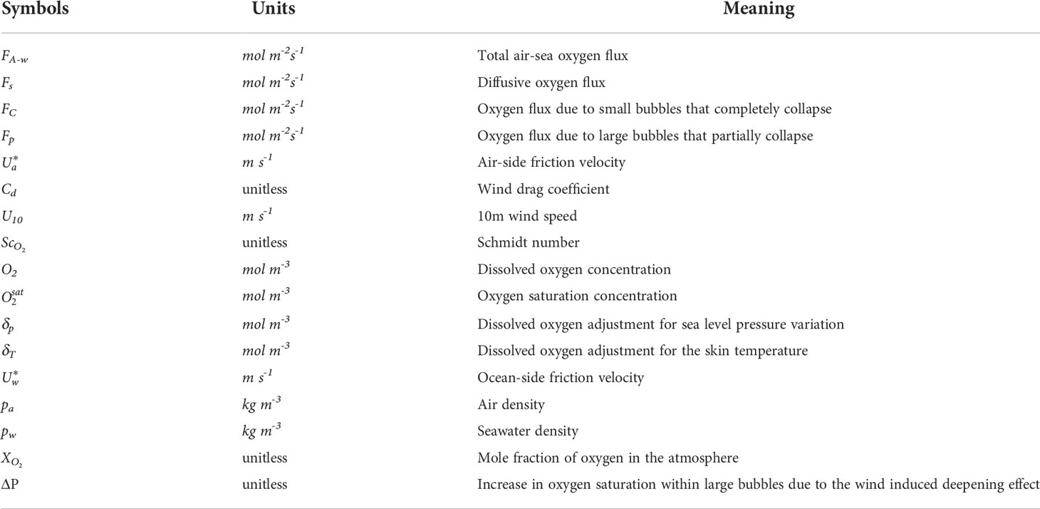
Table 1 The meaning of symbols used in Section 2.4.2 and their units.
Most seasonal variability of the MLD occurs in the extra-tropics and subpolar regions within the 30° to 70° latitude belt of the Northern Hemisphere (NH) and Southern Hemisphere (SH) (Figure 1). In the NH, the largest (deepest) MLD is found in the Atlantic Ocean (Figures 1B, E) with depths greater than 1000m, which occurs around 60°N in March. The mixed layer starts to become shallower in April and rapidly decreases to less than 40 m on average in June. The average MLD remains shallower than 50 m between June and September for the global ocean and in each of the major ocean basins. The deepening of the ML starts in September and continues until it reaches the maximum value once again in March. The MLD in the SH shows a similar annual cycle, but differs by six months. The largest annual variation in the SH occurs in the Southern Ocean. The basin MLD climatology (Figures 1B–D, G–I) shows basin scale differences among the three basins. A full-cycle deep ML belt is formed in the Southern Ocean during SH winter between 40 and 60°S (spatial plots, not shown). The belt is shallowest in the Atlantic Ocean and deepest in the Pacific Ocean. The center location of the Southern Ocean ML belt is around 40° S in the Indian Ocean (Figure 1C) and shifts to 51°S in the Pacific Ocean (Figure 1D). The belt is much shallower in the Atlantic Ocean centered around 53°S. The monthly time series of average MLD climatologies between 30° and 70° in Figures 1F–I also shows a strong annual cycle in the subtropics and subpolar regions.
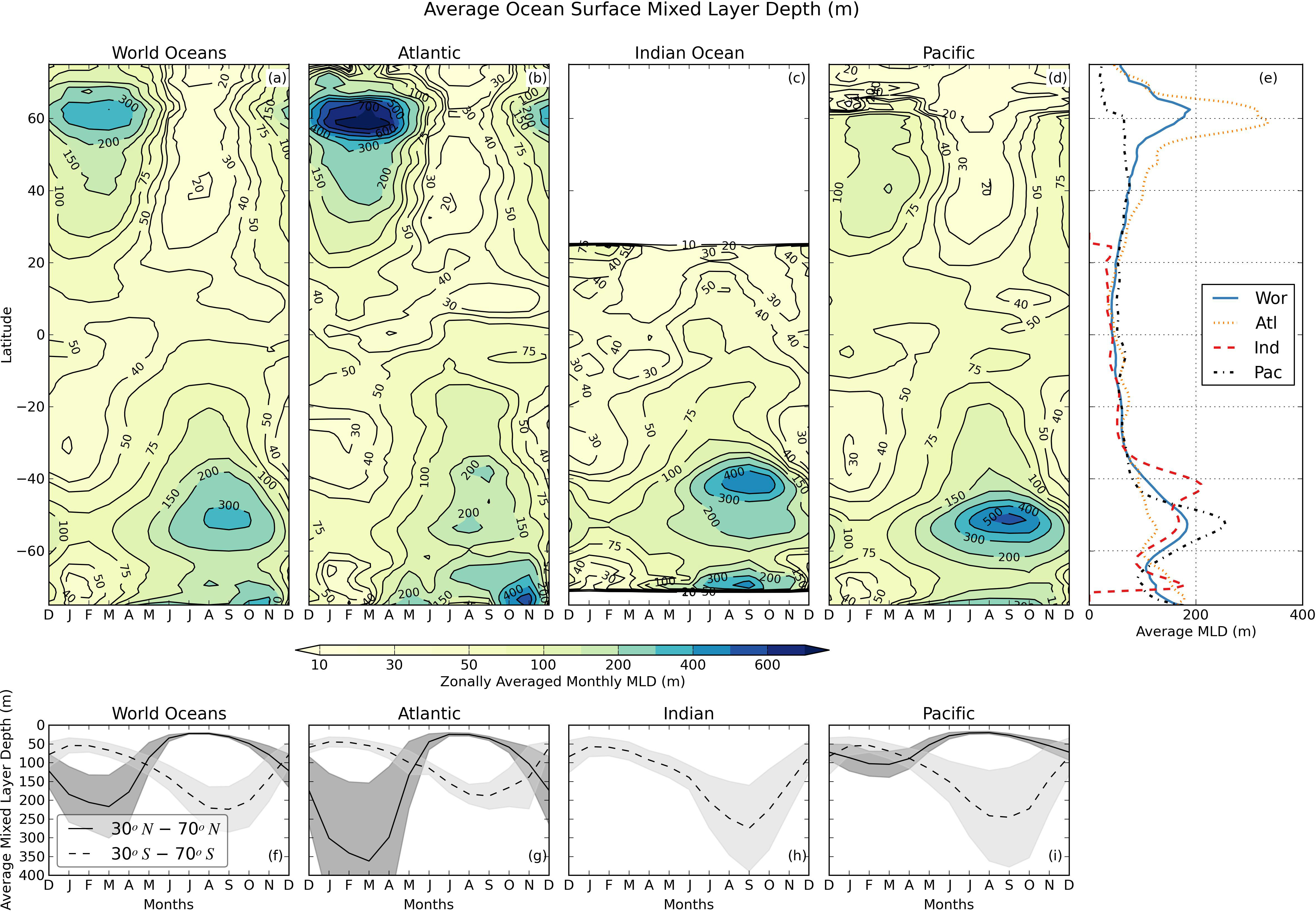
Figure 1 Average climatology of mixed layer depth (MLD) in meters. Zonally averaged monthly MLD for the (A) World, (B) Atlantic, (C) Indian, and (D) Pacific Ocean. Same colorbar is used for panels (A–D) as shown below them. The contour lines are 20, 30, 40, 50, 75, 100, 150, 200, 300, 400, 500, 600 and 700m. (E) Zonal and annual average of MLD as a function of latitude for the World Ocean and the three major ocean basins. Zonally averaged monthly time series estimate of the mixed layer depth for the subtropics and mid-latitudes between 30° and 70° for both Northern Hemisphere (NH, solid black) and Southern Hemisphere (SH, dashed black) for (F) World, (G) Atlantic, (H) Indian, and (I) Pacific Ocean, respectively. The shadow areas in (F–I) represent the data variability between one standard deviation (SD) above and one standard deviation below the average. The standard deviation is estimated based on the zonal averages shown in the plots (A–D) above.
Similar to the MLD seasonal variations, the largest seasonal changes in O2C also occur in the extra-tropics and subpolar regions between 30° and 70° of the NH and SH (Figure 2). In the NH, the largest seasonal peak (>110.0 mol/m2) occurs between February and April and centered near 60°N (Figure 2A), which is when and where the MLD is deepest in the NH (Figure 1). The smallest O2C (<10.0 mol/m2) occurs during summer between July and September in the NH. In the SH, the largest seasonal peak occurs approximately in September and centered at 55°S in the southern Pacific Ocean. The magnitude of the SH peak (~90.0 mol/m2) for the global ocean is slightly smaller than that of the NH. The center locations of the Southern Ocean O2C peaks in the three basins (Figures 2B, C) are consistent with the center locations of the deepest MLD shown in Figure 1. In the tropical and subtropical regions, the seasonal variations are smaller compared to those in high latitudes. As would be expected, the seasonal and spatial variations of the ML O2C for both global and the three major basins (Figure 2) are highly correlated with the seasonal and spatial distributions of the MLD (Figure 1) by comparing the two figures. In the northern Atlantic and southern Pacific, the mixed layer has larger seasonal variations and can hold 10+ times more O2 content in the winter than that in the summer. Although MLD plays a dominant role in determining the peak O2C in the winter, the O2 concentration might be also larger in the winter than that in the fall due to enhanced air-sea flux and thermal-induced solubility increase (Najjar and Keeling, 1997; Najjar and Keeling, 2000; Garcia et al., 2005a). The winter O2C peak in the extra-tropics and subpolar results from the combination of mixed layer deepening and O2 solubility increase. The O2C seasonal variation in the northern Pacific is much smaller than that in the northern Atlantic. The annual averaged O2C in Figure 2E also shows huge spatial differences among different basins and the global ocean.
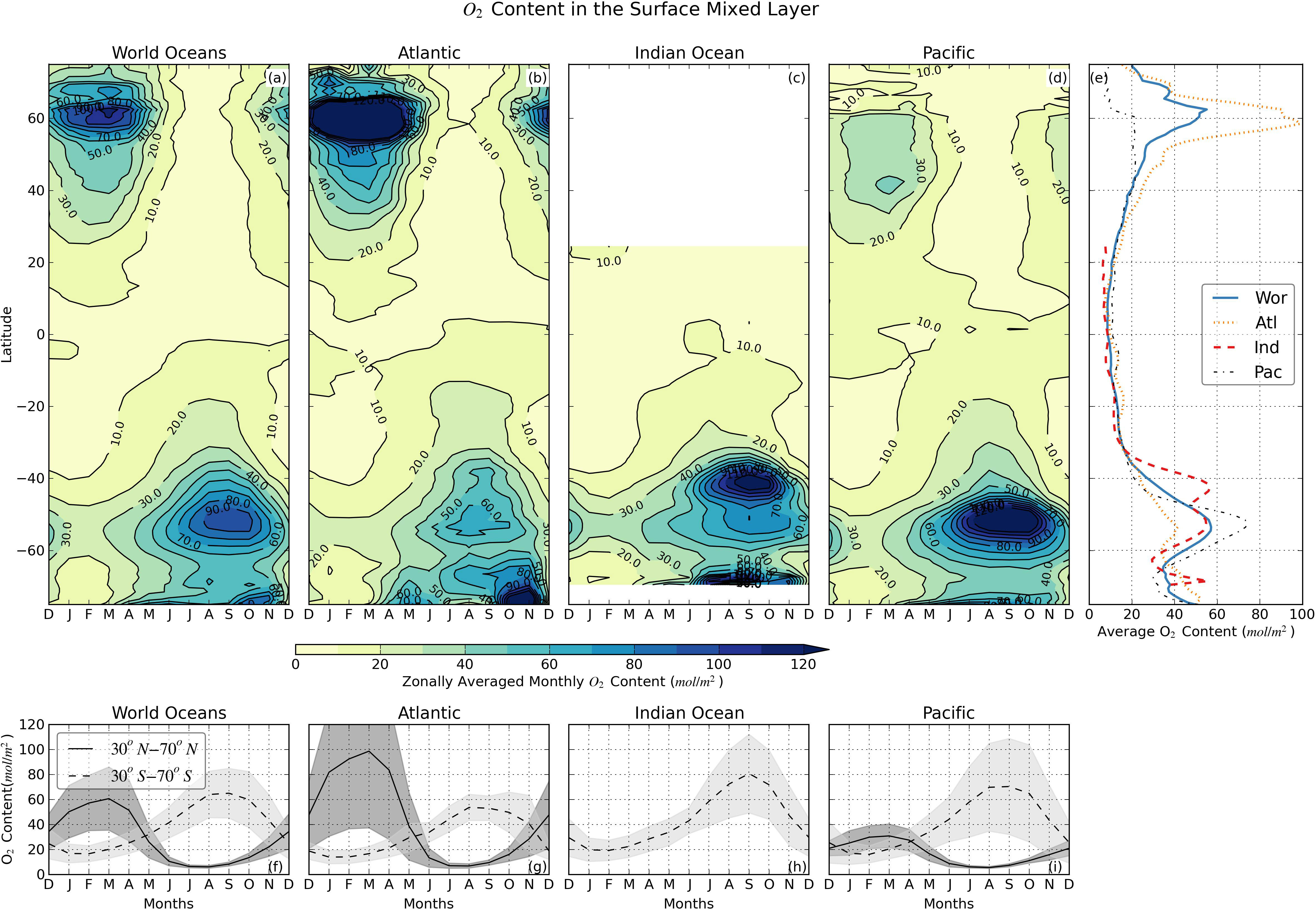
Figure 2 Climatology of area-averaged O2C in the surface mixed layer (mol/m2). Zonally averaged monthly O2C in the mixed layer for the (A) World, (B) Atlantic, (C) Indian, and (D) Pacific Ocean. Same colorbar is used for panels (A–D) as shown below them. The contour interval is 10.0 mol/m2. (E) Annual zonally-averaged O2C for the world ocean and the three major basins. Monthly time series estimate of the O2C between 30° and 70° latitude for the (F) World, (G) Atlantic, (H) Indian and (I) Pacific Ocean, respectively. The shadow areas in (F–I) represent the data variability (±1 SD). Note O2C in this figure is area-averaged to compare the values of the world ocean with the three basins.
Oxygen content shows the total O2 mass variations in the surface mixed layer, which is highly correlated with the mixed layer thickness (depth). The average O2 concentration in the mixed layer, O2m, is a variable that less depends on the mixed layer depth. In Figure 3, we show the zonally-averaged mean O2 concentration in the ML for the global ocean and the three major basins. Interestingly, the seasonal variations and spatial distributions of O2m are very similar for the global ocean and the three major basins (Figures 3A–D), even though their respective O2C distributions (Figure 2) are quite different. The annual averaged O2m for the global and the three basins are also very similar and mostly a function of latitude (Figure 3E). That is because the water in the mixed layer is saturated or near-saturated (O2 saturation >90% in the ML) for the global ocean and the three basins (Figure S1 in the Supplemental Material) throughout the year in the mixed layer and the mean O2 concentration becomes mainly a function of the O2 solubility of the water, which is lowest at tropical regions and increases towards polar regions (Keeling and Garcia, 2002). Although the O2 solubility is a function of temperature and salinity, temperature is the main driver for the latitudinal O2 solubility increase towards polar regions because temperature field in the mixed layer is also a function of latitudes (Boyer et al., 2018; Garcia et al., 2018; Locarnini et al., 2018). The maximum O2m is typically observed in May in the NH and in December or January in the SH (Figures 3F–I) when the oxygen saturation reaches 100% (Figure S1). The minimum O2m usually happens in September in the NH (Figures 2F, G, I). The contour lines for the O2m in the SH are flatter between 30°S and 60°S than those in the NH and the seasonal variations are not as obvious as those for the NH. O2m minimum is observed between September and November south of 60°S (Figure 3), when and where the oxygen saturation is lowest (Figure S1). The time series in Figures 3F-I also showed similarities regarding the seasonal variations in the global and basin averaged O2m.
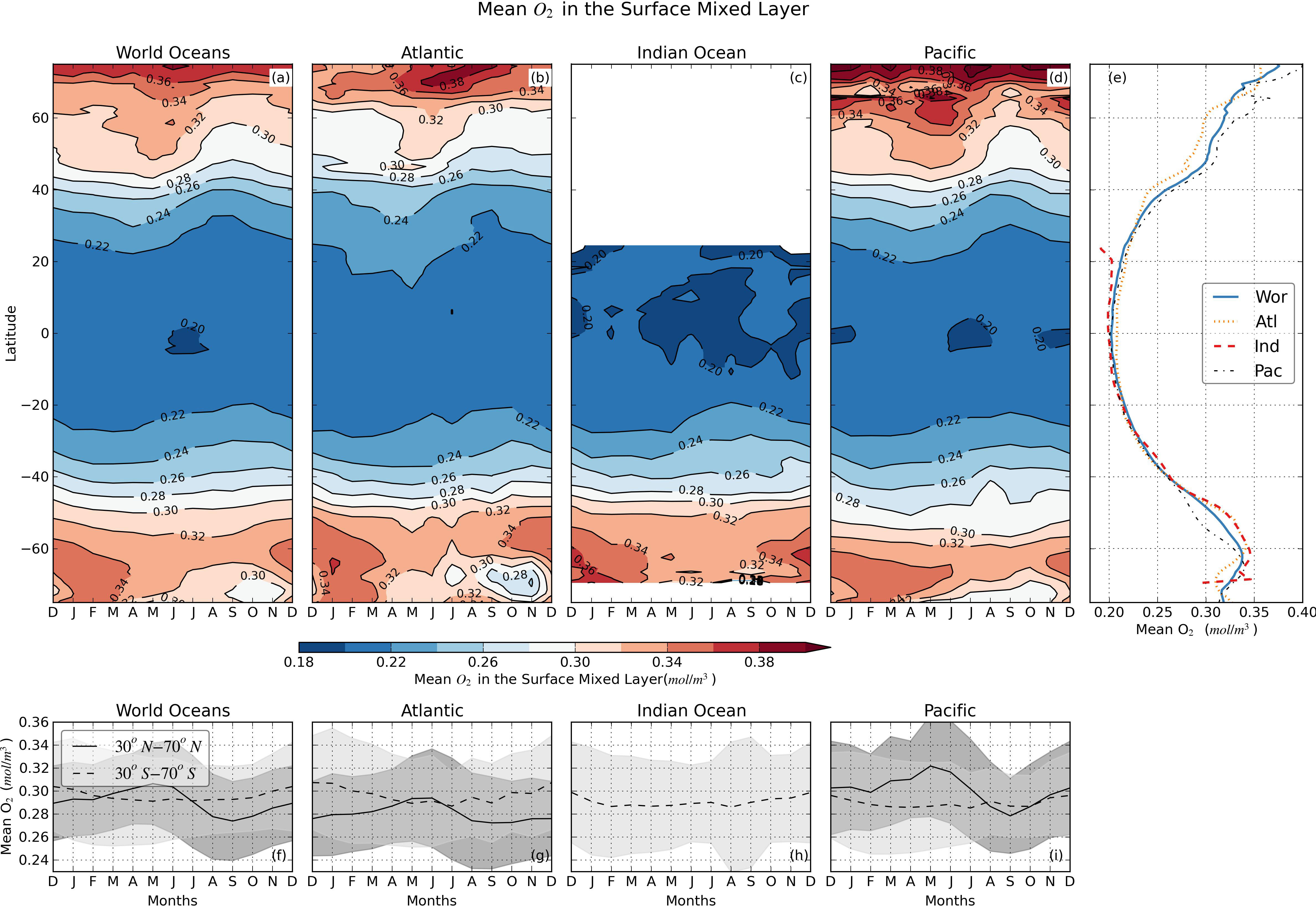
Figure 3 Climatology of mean O2 concentration in the surface ML (mol/m3). Zonally averaged monthly mean oxygen concentration in the surface mixed layer for the (A) World, (B) Atlantic, (C) Indian, and (D) Pacific Ocean. Same colorbar used for panels (A–D) as shown below them. The contour interval is 0.02 mol/m3. (E) Annual zonally averaged oxygen for the world ocean and the three major basins. Monthly time series estimate of the mean oxygen between 30° and 70° for both northern Hemisphere (solid black) and Southern Hemisphere (dashed black) for the (F) World, (G) Atlantic, (H) Indian and (I) Pacific Ocean, respectively. The shadow areas in (F–I) represent the data variability.
In this section, we apply the O2 mass balance model (Section 2.4) to study the controlling factors of O2m and O2C annual cycle for the global ocean. Entrainment, air-sea oxygen flux and “biological” O2 production are the three major controlling factors that are considered in this simple model to examine the relative importance of each factor in each month. Figures 4A–D show the zonally-averaged monthly values for the four terms in Eq. (2). For all the terms examined, positive means adding oxygen to the mixed layer and negative means losing oxygen from the mixed layer, either to the deeper layer or to the atmosphere. In the case of air-sea flux, negative means outgassing and positive ingassing. The seasonality of the four terms is most significant between 30˚ and 70˚ for both NH and SH (Figure 4). At high and mid-latitudes, the oxygen annual cycle can be separated into four stages based on the four terms in Figure 4. During the spring, when the mixed layer depth shoals (Figure 1), the oxygen content begins to decrease with time from the maximum content values (Figures 2A, F, 4A, E). The entrainment term also decreases and weakens to zero due to the shoaling of the mixed layer (Figures 4B, F). The air-sea O2 ingassing weakens and a reversal to outgassing occurs at middle to late spring (Figures 4C, G). The biologically-produced oxygen increases rapidly and peaks in late spring (Figures 4D, H). In the summer, the oxygen content change is slightly negative and small (Figure 4A). The outgassing of oxygen is balanced with the oxygen produced by biological activity (Figure 4). In the fall, outgassing transitions to ingassing due to solubility changes (colder = more soluble) and oxygen starts to transfer downward via entrainment (Figures 4B, C). Biological processes change from a net source (production) to a net sink (consumption). During the winter, the entrainment continues transferring a large amount of oxygen into the deepwater. The biological activity also uses up oxygen in the ML. The air-sea ingassing is the primary source of oxygen in the ML at high and mid-latitudes (>30˚ latitude). In the tropical regions between 30˚S and 30˚N, the annual net oxygen content change and entrainment are near zero (Figure 4I) suggesting that the air-sea flux is nearly balanced by the biological activity and other forcing processes that are not considered in Eq. (2).
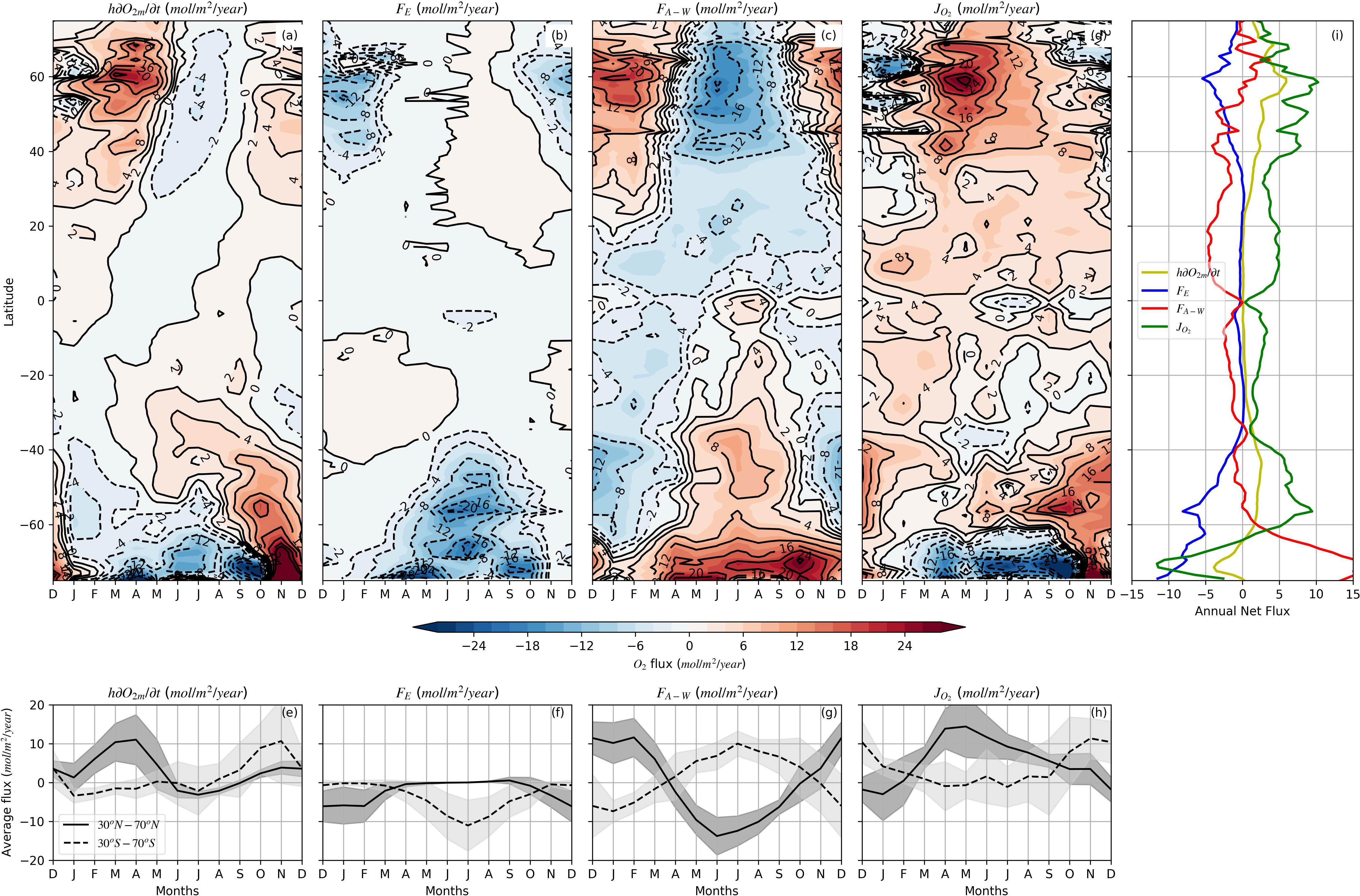
Figure 4 Zonally averaged mixed layer (A) oxygen content change, (B) entrainment, (C) air-sea O2 flux and (D) residuals (“biological” O2 production). Same colorbar is used for panels (A–D) as shown below them. Monthly time series estimate between 30° and 70° for (E) oxygen content change, (F) entrainment, (G) air-sea O2 flux and (H) “biological” O2 production, respectively. (I) Annual zonally-averaged net O2 flux (change) for the terms shown in (A–D). The shadow areas in (E–H) represent the data variability (±1 SD).
In the high and mid-latitudes of the NH, the period of positive oxygen content changes lasts for about 8 months (from September until April, Figure 4A), which yields a net annual oxygen increase in the ML between 25°N and 75°N (Figure 4I). The annual oxygen content change between 25°S and 25°N is about zero. In the SH, the annual oxygen content change is positive between 25°S and 62°S, but negative between 62°S and 75°S. The annual entrainment flux is always negative and only significant in the high and mid-latitudes (Figure 4I). The annual net air-sea O2 flux is predominately ingassing in the high latitudes and outgassing in the mid and low latitudes. The annual net biological O2 production in the ML is positive for most regions of the global ocean except for the high latitudes near Antarctic, suggesting biological activity contributes net O2 to the ML on a global scale.
To better demonstrate the relative importance of the three controlling factors on the right-hand side of Eq. (2), in Figure 5, we replot the monthly time series shown in Figures 4E–H using histograms. Figures 5A, C display the actual flux values in mole m-2 yr-1 in the NH and SH, respectively; while Figures 5B, D show the relative percentage (importance) of the magnitude of the three factors by scaling their total magnitude to 100% in each month. We also superimpose the mixed layer depth on the histograms in Figures 5A, C to show the seasonality of the MLD. In the winter, air-sea flux is the dominant factor, controlling 50%-70% of the oxygen content change in both NH and SH. Biological activity becomes a dominant controlling factor in early spring (50-80%). Between late spring and early fall, the air-sea flux plays a slightly larger role (50-60%) than the biological activity (40-50%). The entrainment effect is only strong from late fall to early spring (contributing to 30%-40% of the O2C change, Figure 5). Air-sea flux is positive (ingassing) in the winter and negative (outgassing) in the summer in most regions (Figure 4C). In most months, it controls 40%-60% of the relative O2C change (Figure 5). Biological activity produces oxygen in spring and summer and consumes oxygen in fall and winter in the ML based on the Jo2 estimate (Figure 4D). Biological activity plays a relatively larger role in the spring/summer (40-50%) than that in the fall/winter (10-30%, Figure 5).
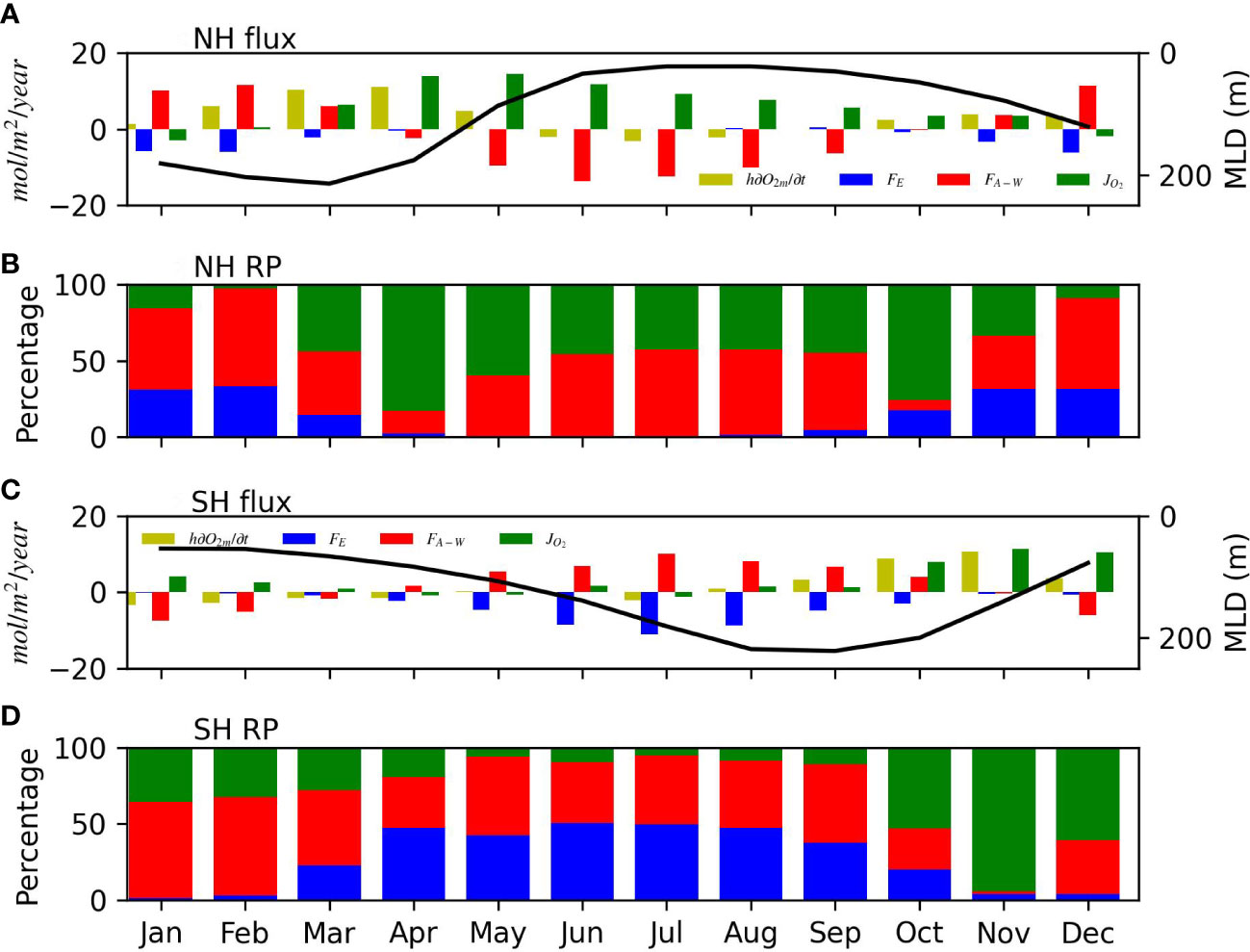
Figure 5 (A) Monthly bar-chart of the four terms in Eq. (2) for the Northern Hemisphere (NH) between 30°N and 70°N. This is a replot of the monthly time series shown in Figures 4E–H. Superimposed black line is the average mixed layer depth between 30°N and 70°N to show the seasonality of the MLD with the four terms. (B) Relative percentage (RP) of the magnitude (absolute value) of the three terms on the right-hand side of Eq. (2) to show the relative importance of each term in controlling O2C change in each month in the NH between 30°N and 70°N. Blue: entrainment, red: air-sea flux, and green: “biological” oxygen production. (C) Monthly bar-chart of the four terms in Eq. (2) for the Southern Hemisphere (SH) between 30°S and 70°S. Similar notations are used as in (A). (D) RP of the magnitude of the three terms in Eq. (2) between 30°S and 70°S. Similar notations are used as in (B).
Based on the above analysis, the oxygen content and O2m annual cycle in the surface mixed layer is controlled by multiple complicated processes that non-linearly correlated with the mixed layer depth. Some of the processes are directly related to the mixed layer depth annual cycle (e.g. entrainment). However, some of the processes are more determined by other factors (e.g. air-sea flux and biological activity), which only indirectly relate to the mixed layer depth changes. The thickness of the mixed layer is determined by wind forcing and heating from the atmosphere. Wind forcing is also a key parameter determining the air-sea oxygen flux at sea surface (see Section 2.4.2). Heating from the atmosphere affects the water temperature, which further affects the oxygen solubility and mixed layer depth. Variations in mixed layer affect the rate of air-sea oxygen flux between the atmosphere and deeper ocean, the capability of the ocean to store oxygen and nutrient supplies to support the growth of phytoplankton. All these processes interact each other and build up complex linkages between mixed layer depth and oxygen concentration/content annual cycle in the upper ocean. The simple mass balance model effectively demonstrates the relative importance of the three essential factors in different seasons for the upper ocean oxygen dynamics in the global ocean. This is also valuable for improving our understanding of overall biology activity in the surface mixed layer. In the following section, we will discuss more about biologically-produced oxygen and relate it to the net community production in the mixed layer for the global ocean.
The seasonality of JO2 follows our traditional understanding of biologically-produced oxygen patterns (producing oxygen in spring/summer and consuming oxygen in fall/winter). However, it is difficult to directly validate the JO2 estimates due to the lack of biological O2 production observations in the mixed layer for the global ocean. We convert JO2 to net community production (NCP) following Craig and Hayward (1987); Emerson (1987); Spitzer and Jenkins (1989); Emerson et al. (2008) and Yang et al. (2017) and compare our results with previous NCP estimates. Assuming a ΔO2:ΔC ratio of 1.45 (Hedges et al., 2002; Emerson and Stump, 2010; Bushinsky and Emerson, 2015), JO2 is converted to NCP and shown in Figure 6. Our estimates in Figure 6 provide a global view of the seasonal variations of the NCP for the world ocean based on the oxygen mass balance. Our estimates of zonal annual net community production (ANCP, Figure 6B) range from approximately 0.5 mol C m-2 year-1 to ~6.0 mol C m-2 year-1 except for south of 60˚S, which can be less than -5.0 mol C m-2 year-1. NCP in mid and high latitudes is largest in the spring and smallest in the winter (Figures 6A, C), consistent with the typical seasonal biological activity in the ocean. The global average ANCP is 3.06±1.61 mol C m-2 year-1 (mean±SD) between 60˚S and 60˚N. The average ANCP in the NH between 0 and 60˚N is 3.69±1.38 mol C m-2 year-1, which is much larger than the average value (2.41 ±1.57 mol C m-2 year-1) in the SH (0-60 ˚S). Similar hemispheric asymmetry has been reported in Quay et al. (2009) in the Pacific with subtropical ANCP in the north Pacific (2.6±0.6 mol C m-2 year-1) being twice that in the South Pacific (1.3±0.4 mol C m-2 year-1). Our results suggest the ANCP hemispheric asymmetry may be a global phenomenon. The causes of asymmetric ANCP distribution between NH and SH are unclear and could inspire further investigation. Our global average ANCP estimates are comparable to previous studies at fixed stations or in regional seas. ANCP at different long-term fixed stations are estimated to be from 1.9-3.8 mol C m-2 yr-1 from 10+ year time series (Keeling et al., 2004; Emerson, 2014). Stanley et al. (2010) calculated the mean NCP in the equatorial Pacific to be 1.2~1.5 mol C m-2 yr-1 based on data from a 2-month summer cruise. Yang et al. (2017) estimated the ANCP in the subtropical Pacific Ocean to be 0~2.4 mol C m-2 yr-1 using Argo oxygen data. ANCP estimates based on models range from 1.0 to 5.7 mol C m-2 yr-1, while satellite-based ANCP estimates range from 1.5 to 3.8 mol C m-2 yr-1 (Emerson, 2014). Haskell et al. (2020) reported similar total carbon export out of the euphotic zone (ANCP) of 3.2±0.6 to 4.5±0.5 mol C m-2 yr-1. Note, unlike using a variable mixed layer depth as in this study, in the previous ANCP estimates, fixed integral depth (e.g. deepest annual MLD, euphotic zone) is often used in the ANCP estimates, which makes it difficult to conduct a direct comparison among studies because different integral depths are used. Moreover, different assumptions and equations were used in different estimate methods, which makes the comparison further complicated. Nonetheless, all these estimates are for the ANCP in the upper ocean and a rough comparison can be still conducted by comparing the range and trend in different estimates. Large discrepancies might be seen when comparing ANCP from different estimate methods. Keep in mind, the ANCP estimated in this study is the ANCP within the mixed layer of the global ocean. A portion of the annual productivity between summer MLD and euphotic depth is not included in our ANCP estimate when the MLD is shallower than the euphotic depth.
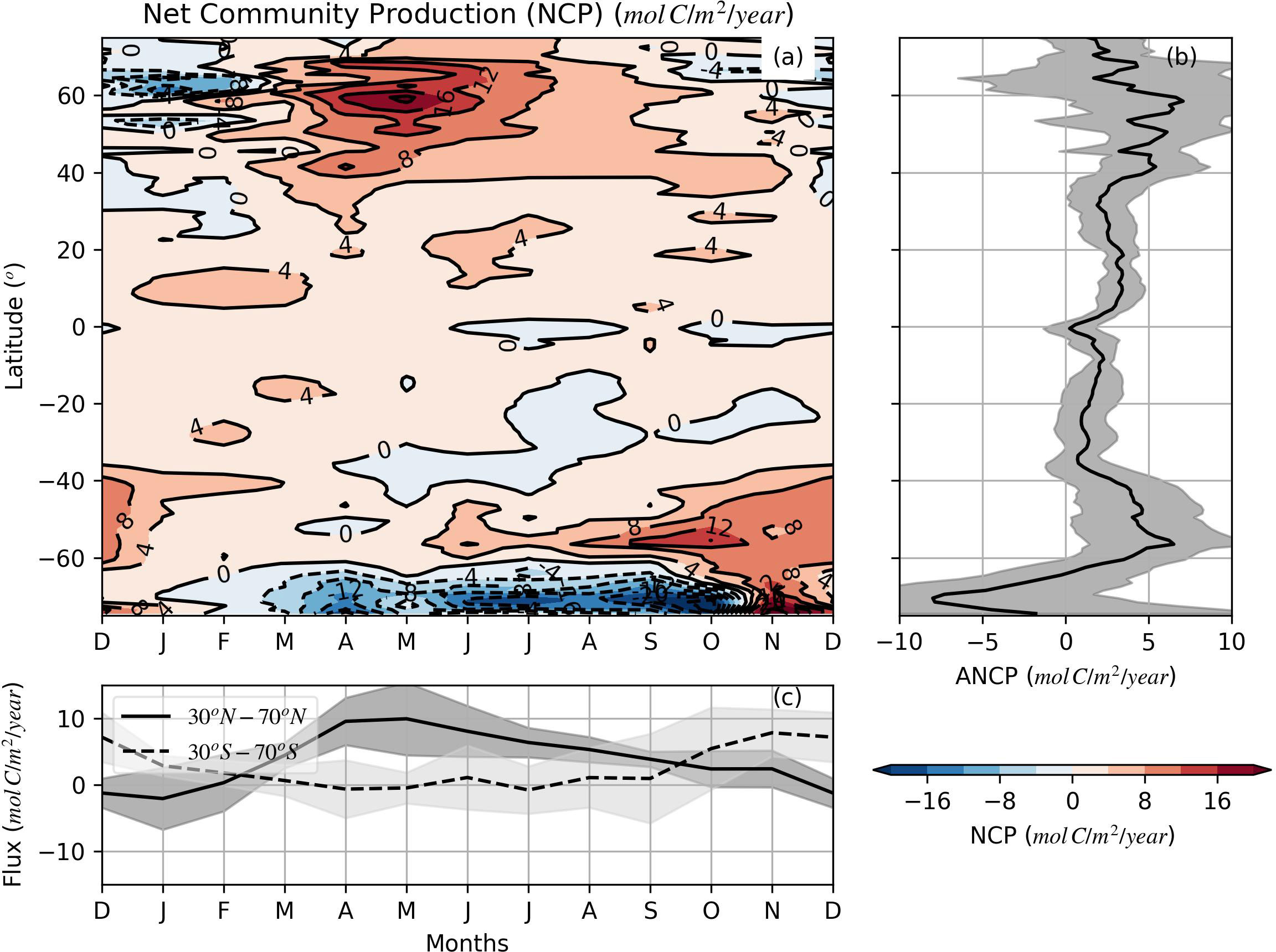
Figure 6 (A) Zonally averaged mixed layer net community production (NCP) determined by the O2 mass balance model. (B) Zonally-averaged annual net community production (ANCP). (C) Monthly time series estimate of NCP between 30° and 70° for both NH and SH. The shadow areas in (B, C) represent the data variability (±1 SD).
From our mass balance model, the global ANCP (60˚S-60˚N) in the mixed layer is estimated at 859.7±73.8 Tmol C yr-1, which is slightly larger than the estimate (781±393 Tmol C yr-1) from a satellite-based model in the euphotic zone (Westberry et al., 2012). ANCP is difficult to quantify on a global scale and estimates of ANCP (or sometimes carbon export production) based on different methods vary considerably, from 250 to more than 2800 Tmol C yr-1 (Sherr and Sherr, 1996; Laws et al., 2000; del Giorgio and Duarte, 2002; Najjar et al., 2007; Emerson, 2014). Our global ANCP estimate is within the range, but close to the lower end compared to some of the previous estimates. This is likely due to the fact that a larger criterion (0.125 kg m-3) is used in our MLD definition. Integrating over a larger mixed layer thickness may include more community respiration in our calculation than some of the previous studies using 0.03 kg m-3 as their MLD criterion or surface satellite-based observations.
In the SH, between 30˚S and 60˚S, our ANCP estimates agree with previous calculations in Johnson et al. (2017) and Arteaga et al. (2019) in demonstrating a low value in subtropical region (30˚S-40˚S) and an increase in ANCP in the Polar Front Zone and Polar Arctic Zone (40˚S-55˚S, Figure 6B). Our negative JO2 and ANCP estimate near Antarctic with latitudes greater than 62˚S (Southern Seasonal Ice Zone) is consistent with the estimate in Trucco-Pignata et al. (2022) in the southeast Pacific, but quite different than that in Johnson et al. (2017), Arteaga et al. (2019) and Yang et al. (2021). Although the lowest, but still positive ANCP (1-2 mol C m-2 yr-1) was calculated by Johnson et al. (2017) and Arteaga et al. (2019) between 60˚S and 70˚S. Omitting diapycnal eddy diffusion might be one of the reasons why a negative value is calculated in our ANCP in the Seasonal Ice Zone, south of 62˚S. Yang et al. (2021) found the diapycnal eddy diffusion played an important role in determining the net annual mixed layer dissolved inorganic carbon on the West Antarctic Peninsula Shelf based on annual carbon budget from a subsurface mooring. Another reason of the negative ANCP might be associated with the large amplitude ingassing air-sea O2 flux (Figure 4). The Southern Ocean is an O2 unsaturated area throughout the year (Figure S1), which makes the diffusive O2 flux ingassing year-long (Ito et al., 2004). The magnitude of the wind is also relatively large throughout the year in that region, which helps the bubble induced O2 into the ocean. More investigation and observational data are needed to further examine the ANCP in the Southern Seasonal Ice Zone.
Despite the overall consistency of the seasonal variations in oxygen content and ANCP with former studies, there are a number of improvements that are needed and there are limitations in this simple oxygen mass balance model. Our air-sea oxygen flux is an update to the estimate made by Najjar and Keeling (2000). 20 more years of oxygen data collected after Najjar and Keeling (2000) paper are added in deriving the WOA18 oxygen climatology. The most updated wind fields, sea surface pressure and sea surface skin temperature monthly climatologies are used in our calculations, which should be more accurate benefiting from the development in satellite observations in recent 20 years. Furthermore, new bubble models that recently developed by Liang et al. (2013) and further improved by Emerson et al. (2019) are used to estimate the bubble-mediated oxygen ingassing, which is a significant improvement in estimation of air-sea gas flux. However, although Garcia et al. (2010) showed the standard error of data used to derive the WOA climatology in the majority of the open ocean could reach to 1-2%Sat, the accuracy of WOA18 oxygen climatology may still not high enough to precisely capture the fine-scale air-sea gas flux (Takeshita et al., 2013). The global oxygen observations to date are still too sparse, especially during winter time and in high latitudes. More observations are needed to improve the accuracy of WOA oxygen climatology.
In this simple model, both diapycnal and horizontal diffusion effects are not considered which might cause uncertainties and errors in the JO2 calculation. Larger turbulent diapycnal mixing is estimated during fall/winter than that in spring/summer, suggesting seasonal variations might exist in turbulent diffusivity based on heat and salt budgets in the North Pacific (Cronin et al., 2015). This also suggests that the errors due to ignorance of diapycnal mixing might be larger in fall/winter. Ignoring the horizontal advection and diffusion term in the model might also cause large errors/uncertainties in the frontal regions (e.g. Kuroshio Extension, Bushinsky and Emerson, 2018), which should be considered when studying the finer-scale studies in addition to the basin-wide and global-scale analyses. The uncertainties and errors in the O2 climatology, wind and current fields may also affect the JO2 estimates, especially in the regions with sparse O2 observations. A full oxygen mass budget may be needed in the future to evaluate the advection, diffusion and other effects (e.g. as in Bushinsky and Emerson, 2015; Bushinsky and Emerson, 2018) for the global ocean.
The spatial and seasonal evolutions of O2C and O2m in the surface ML are determined for the global ocean and the three major basins. An O2 mass balance model is utilized to quantify the entrainment, air-sea flux and biological activity in controlling the seasonal O2 content/concentration change. Based on the mass balance, from mid-fall until early spring in mid and high latitudes, the ML oxygen change is dominated by ingassing from air-sea flux and oxygen loss due to entrainment and biological consumption. The oxygen content change reaches a maximum in the spring due to increased biological oxygen production, while entrainment vanishes and air-sea exchange transitions from ingassing to outgassing. The oxygen content decreases with time due to the strong outgassing in the summer, which overcomes the oxygen produced by biological activity. The entrainment effect is insignificant in the summer. The model estimated mean ANCP ranges from ~0.5 mol C m-2 year-1 to ~6.0 mol C m-2 year-1 with an average value of 3.06±1.61 mol C m-2 year-1 between 60˚S and 60˚N latitude, comparable to previous estimates. The global ANCP is estimated at approximately 863.7±73.8 Tmol C yr-1, which is in good agreement with the estimate (781±393 Tmol C yr-1) based on the photosynthesis/respiration ratio and satellite-based observations (Westberry et al., 2012). The analyses presented here provide a global view at the factors controlling the oxygen concentration in the surface mixed layer and also provide a global estimate of the annual net community production based on the oxygen mass balance.
The original contributions presented in the study are included in the article/Supplementary Material. Further inquiries can be directed to the corresponding author.
ZW and HG contributed to conception and design of the study. ZW conducted mass balance model development and data analysis. JR developed the mixed layer depth climatology. TB and HG led the WOD and WOA management and updates. ZW wrote the first draft of the manuscript. JC contributed to funding acquisition. All authors contributed to the article and approved the submitted version.
This study was supported by NOAA NCEI and a NOAA grant 363541-191001-021000 (Northern Gulf Institute) at Mississippi State University.
The authors would like to thank the scientists and data providers for continuing to share their data, data managers and our NCEI colleagues for stewarding the data for long-term preservation, and the Ocean Climate Laboratory colleagues for continuing to enhance and maintain the WOD and WOA. Without this combined effort, data-based studies like this would not be possible. We thank Y. Lau for helping on air-sea oxygen flux calculation. We thank S. Cross, C. Paver, C. Bouchard, K. Larsen, H. Zhang and other NCEI colleagues for valuable conversations and comments.
The authors declare that the research was conducted in the absence of any commercial or financial relationships that could be construed as a potential conflict of interest.
All claims expressed in this article are solely those of the authors and do not necessarily represent those of their affiliated organizations, or those of the publisher, the editors and the reviewers. Any product that may be evaluated in this article, or claim that may be made by its manufacturer, is not guaranteed or endorsed by the publisher.
The Supplementary Material for this article can be found online at: https://www.frontiersin.org/articles/10.3389/fmars.2022.1001095/full#supplementary-material
Andreev A. G., Baturina V. I. (2006). Impacts of tides and atmospheric forcing variability on dissolved oxygen in the subarctic north pacific. J. Geophys. Res.: Oceans 111 (C07S10), 1–11. doi: 10.1029/2005JC003103
Arteaga L. A., Pahlow M., Bushinsky S. M., Sarmiento J. L. (2019). Nutrient controls on export production in the southern ocean. Global Biogeochem. Cycles 33 (8), 942–956. doi: 10.1029/2019GB006236
Barnes S. L. (1964). A technique for maximizing details in numerical weather map analysis. J. Appl. Meteorol. Climatol. 3 (4), 396–409. doi: 10.1175/1520-0450(1964)003<0396:ATFMDI>2.0.CO;2
Boyer T. P., Baranova O. K., Coleman C., Garcia H. E., Grodsky A., Locarnini R. A., et al. (2018). World Ocean Atlas 2018. NOAA Atlas NESDIS 87, 1–207.
Bushinsky S. M., Emerson S. (2015). Marine biological production from in situ oxygen measurements on a profiling float in the subarctic pacific ocean. Global Biogeochem. Cycles 29 (12), 2050–2060. doi: 10.1002/2015GB005251
Bushinsky S. M., Gray A. R., Johnson K. S., Sarmiento J. L. (2017). Oxygen in the southern ocean from argo floats: Determination of processes driving air-sea fluxes. J. Geophys. Res.: Oceans 122 (11), 8661–8682. doi: 10.1002/2017JC012923
Bushinsky S. M., Emerson S. R. (2018). Biological and physical controls on the oxygen cycle in the kuroshio extension from an array of profiling floats. Deep Sea Res. Part I: Oceanogr. Res. Papers 141, 51–70. doi: 10.1016/j.dsr.2018.09.005
Craig H., Hayward T. (1987). Oxygen supersaturation in the ocean: Biological versus physical contributions. Science 235 (4785), 199–202. doi: 10.1126/science.235.4785.199
Cronin M. F., Pelland N. A., Emerson S. R., Crawford W. R. (2015). Estimating diffusivity from the mixed layer heat and salt balances in the north pacific. J. Geophys. Res.: Oceans 120 (11), 7346–7362. doi: 10.1002/2015JC011010
de Boyer Montégut C., Madec G., Fischer A. S., Lazar A., Iudicone D. (2004). Mixed layer depth over the global ocean: An examination of profile data and a profile-based climatology. J. Geophys. Res.: Oceans 109 (C12), 1–20. doi: 10.1029/2004JC002378
del Giorgio P. A., Duarte C. M. (2002). Respiration in the open ocean. Nature 420 (6914), 379–384. doi: 10.1038/nature01165
Emerson S. (1987). Seasonal oxygen cycles and biological new production in surface waters of the subarctic pacific ocean. J. Geophys. Res.: Oceans 92 (C6), 6535–6544. doi: 10.1029/JC092iC06p06535
Emerson S. (2014). Annual net community production and the biological carbon flux in the ocean. Global Biogeochem. Cycles 28 (1), 14–28. doi: 10.1002/2013GB004680
Emerson S., Bushinsky S. (2016). The role of bubbles during air-sea gas exchange. J. Geophys. Res.: Oceans 121 (6), 4360–4376. doi: 10.1002/2016JC011744
Emerson S., Stump C. (2010). Net biological oxygen production in the ocean–II: Remote in situ measurements of O2 and N2 in subarctic pacific surface waters. Deep Sea Res. Part I: Oceanogr. Res. Papers 57 (10), 1255–1265. doi: 10.1016/j.dsr.2010.06.001
Emerson S., Stump C., Nicholson D. (2008). Net biological oxygen production in the ocean: Remote in situ measurements of O2 and N2 in surface waters. Global Biogeochem. Cycles 22 (3), 1–13. doi: 10.1029/2007GB003095
Emerson S., Yang B., White M., Cronin M. (2019). Air-sea gas transfer: Determining bubble fluxes with in situ N2 observations. J. Geophys. Res.: Oceans 124 (4), 2716–2727. doi: 10.1029/2018JC014786
Garcia H. E., Boyer T. P., Levitus S., Locarnini R. A., Antonov J. I. (2005a). Climatological annual cycle of upper ocean oxygen content anomaly. Geophys. Res. Lett. 32 (5), 1–4. doi: 10.1029/2004GL021745
Garcia H. E., Boyer T. P., Levitus S., Locarnini R. A., Antonov J. (2005b). On the variability of dissolved oxygen and apparent oxygen utilization content for the upper world ocean: 1955 to 1998. Geophys. Res. Lett. 32 (9), 1–4. doi: 10.1029/2004GL022286
Garcia H. E., Gordon L. I. (1992). Oxygen solubility in seawater: Better fitting equations. Limnol. oceanogr. 37 (6), 1307–1312. doi: 10.4319/lo.1992.37.6.1307
Garcia H. E., Keeling R. F. (2001). On the global oxygen anomaly and air-sea flux. J. Geophys. Res.: Oceans 106 (C12), 31155–31166. doi: 10.1029/1999JC000200
Garcia H. E., Locarnini R. A., Boyer T. P., Antonov J. I., Baranova O. K., Zweng M. M., et al. (2010). World Ocean Atlas 2009, Volume 3: Dissolved Oxygen, Apparent Oxygen Utilization, and Oxygen Saturation, NOAA Atlas NESDIS 70, edited by Levitus S. U.S. Gov. Print. Off., Washington, D. C.
Garcia H. E., Weathers K., Paver C. R., Smolyar I., Boyer T. P., Locarnini R. A., et al. (2018). World ocean atlas 2018, volume 3: Dissolved oxygen, apparent oxygen utilization, and oxygen Saturation.A. mishonov technical ed.;. NOAA Atlas NESDIS 83, 38.
Haskell W. Z., Fassbender A. J., Long J. S., Plant J. N. (2020). Annual net community production of particulate and dissolved organic carbon from a decade of biogeochemical profiling float observations in the northeast pacific. Global Biogeochem. Cycles 34 (10), e2020GB006599. doi: 10.1029/2020GB006599
Hedges J. I., Baldock J. A., Gélinas Y., Lee C., Peterson M. L., Wakeham S. G. (2002). The biochemical and elemental compositions of marine plankton: A NMR perspective. Mar. Chem. 78 (1), 47–63. doi: 10.1016/S0304-4203(02)00009-9
Huang Y., Fassbender A. J., Long J. S., Johannessen S., Bernardi Bif M. (2022). Partitioning the export of distinct biogenic carbon pools in the northeast pacific ocean using a biogeochemical profiling float. Global Biogeochem. Cycles 36 (2), e2021GB007178. doi: 10.1029/2021GB007178
IOC, SCOR and IAPSO (2010). The international thermodynamic equation of seawater–2010: Calculation and use of thermodynamic properties, intergovernmental oceanographic commission, manuals and guides no. 56. UNESCO Manuals Guides 56, 1–196.
Ito T., Follows M. J., Boyle E. A. (2004). Is AOU a good measure of respiration in the oceans? Geophys. Res. Lett. 31 (17), 1–4. doi: 10.1029/2004GL020900
Ito T., Long M. C., Deutsch C., Minobe S., Sun D. (2019). Mechanisms of low-frequency oxygen variability in the north pacific. Global Biogeochem. Cycles 33 (2), 110–124. doi: 10.1029/2018GB005987
Ito T., Minobe S., Long M. C., Deutsch C. (2017). Upper ocean O2 trends: 1958–2015. Geophys. Res. Lett. 44 (9), 4214–4223. doi: 10.1002/2017GL073613
Ito T., Takano Y., Deutsch C., Long M. C. (2022). Sensitivity of global ocean deoxygenation to vertical and isopycnal mixing in an ocean biogeochemistry model. Global Biogeochem. Cycles 36 (4), e2021GB007151. doi: 10.1029/2021GB007151
Jin X., Najjar R. G., Louanchi F., Doney S. C. (2007). A modeling study of the seasonal oxygen budget of the global ocean. J. Geophys. Res.: Oceans 112 (C05017), 1–19. doi: 10.1029/2006JC003731
Johnson K. S., Plant J. N., Dunne J. P., Talley L. D., Sarmiento J. L. (2017). Annual nitrate drawdown observed by SOCCOM profiling floats and the relationship to annual net community production. J. Geophys. Res.: Oceans 122 (8), 6668–6683. doi: 10.1002/2017JC012839
Kara A. B., Rochford P. A., Hurlburt ,. H. E. (2000). An optimal definition for ocean mixed layer depth. J. Geophys. Res. 105 (C7), 16803–16821. doi: 10.1029/2000JC900072
Kara A. B., Wallcraft A. J., Metzger E. J., Hurlburt H. E., Fairall C. W. (2007). Wind stress drag coefficient over the global ocean. J. Climate 20 (23), 5856–5864. doi: 10.1175/2007JCLI1825.1
Keeling C. D., Brix H., Gruber N. (2004). Seasonal and long-term dynamics of the upper ocean carbon cycle at station ALOHA near Hawaii. Global Biogeochem. Cycles 18 (4), 1–26. doi: 10.1029/2004GB002227
Keeling R. F., Garcia H. E. (2002). The change in oceanic O2 inventory associated with recent global warming. Proc. Natl. Acad. Sci. 99 (12), 7848–7853. doi: 10.1073/pnas.122154899
Keeling R. F., Shertz S. R. (1992). Seasonal and interannual variations in atmospheric oxygen and implications for the global carbon cycle. Nature 358 (6389), 723–727. doi: 10.1038/358723a0
Large W. G., Pond S. (1981). Open ocean momentum flux measurements in moderate to strong winds. J. Phys. oceanogr. 11 (3), 324–336. doi: 10.1175/1520-0485(1981)011<0324:OOMFMI>2.0.CO;2
Laws E. A., Falkowski P. G., Smith W. O. Jr., Ducklow H., McCarthy J. J. (2000). Temperature effects on export production in the open ocean. Global biogeochem. cycles 14 (4), 1231–1246. doi: 10.1029/1999GB001229
Liang J. H., Deutsch C., McWilliams J. C., Baschek B., Sullivan P. P., Chiba D. (2013). Parameterizing bubble-mediated air-sea gas exchange and its effect on ocean ventilation. Global Biogeochem. Cycles 27 (3), 894–905. doi: 10.1002/gbc.20080
Locarnini R. A., Mishonov A. V., Baranova O. K., Boyer T. P., Zweng M. M., Garcia H. E., et al. (2018). World ocean atlas 2018, volume 1: Temperature.A. mishonov technical ed.;. NOAA Atlas NESDIS 81, 52.
Manizza M., Keeling R. F., Nevison C. D. (2012). On the processes controlling the seasonal cycles of the air–sea fluxes of O2 and N2O: A modelling study. Tellus B: Chem. Phys. Meteorol. 64 (1), 18429. doi: 10.3402/tellusb.v64i0.18429
McDougall T. J., Barker P. M. (2011). Getting started with TEOS-10 and the Gibbs seawater (GSW) oceanographic toolbox. SCOR/IAPSO WG. 127, 1–28.
Najjar R. G., Jin X., Louanchi F., Aumont O., Caldeira K., Doney S. C., et al. (2007). Impact of circulation on export production, dissolved organic matter, and dissolved oxygen in the ocean: Results from phase II of the ocean carbon-cycle model intercomparison project (OCMIP-2). Global Biogeochem. Cycles 21 (3), 1–22. doi: 10.1029/2006GB002857
Najjar R. G., Keeling R. F. (1997). Analysis of the mean annual cycle of the dissolved oxygen anomaly in the world ocean. J. Mar. Res. 55 (1), 117–151. doi: 10.1357/0022240973224481
Najjar R. G., Keeling R. F. (2000). Mean annual cycle of the air-sea oxygen flux: A global view. Global biogeochem. cycles 14 (2), 573–584. doi: 10.1029/1999GB900086
Oschlies A., Brandt P., Stramma L., Schmidtko S. (2018). Drivers and mechanisms of ocean deoxygenation. Nat. Geosci. 11 (7), 467–473. doi: 10.1038/s41561-018-0152-2
Quay P., Emerson S., Palevsky H. (2020). Regional pattern of the ocean’s biological pump based on geochemical observations. Geophys. Res. Lett. 47 (14), e2020GL088098. doi: 10.1029/2020GL088098
Ren L., Riser S. C. (2009). Seasonal salt budget in the northeast pacific ocean. J. Geophys. Res.: Oceans 114 (C12), 1–11. doi: 10.1029/2009JC005307
Sherr E. B., Sherr B. F. (1996). Temporal offset in oceanic production and respiration processes implied by seasonal changes in atmospheric oxygen: The role of heterotrophic microbes. Aquat. Microb. Ecol. 11 (1), 91–100. doi: 10.3354/ame011091
Spitzer W. S., Jenkins W. J. (1989). Rates of vertical mixing, gas exchange and new production: Estimates from seasonal gas cycles in the upper ocean near Bermuda. J. Mar. Res. 47 (1), 169–196. doi: 10.1357/002224089785076370
Stanley R. H., Jenkins W. J., Lott D. E. III, Doney S. C. (2009). Noble gas constraints on air-sea gas exchange and bubble fluxes. J. Geophys. Res.: Oceans 114 (C11), 1–14. doi: 10.1029/2009JC005396
Stanley R. H., Kirkpatrick J. B., Cassar N., Barnett B. A., Bender M. L. (2010). Net community production and gross primary production rates in the western equatorial pacific. Global Biogeochem. Cycles 24 (4), 1–17. doi: 10.1029/2009GB003651
Stevenson J. W., Niiler P. P. (1983). Upper ocean heat budget during the Hawaii-to-Tahiti shuttle experiment. J. Phys. oceanogr. 13 (10), 1894–1907. doi: 10.1175/1520-0485(1983)013<1894:UOHBDT>2.0.CO;2
Takeshita Y., Martz T. R., Johnson K. S., Plant J. N., Gilbert D., Riser S. C., et al. (2013). A climatology-based quality control procedure for profiling float oxygen data. J. Geophys. Res.: Oceans 118 (10), 5640–5650. doi: 10.1002/jgrc.20399
Thomson R. E., Fine I. V. (2003). Estimating mixed layer depth from oceanic profile data. J. Atmos. Oceanic Technol. 20 (2), 319–329. doi: 10.1175/1520-0426(2003)020<0319:EMLDFO>2.0.CO;2
Toyoda T., Fujii Y., Kuragano T., Kamachi M., Ishikawa Y., Masuda S., et al. (2017). Intercomparison and validation of the mixed layer depth fields of global ocean syntheses. Climate Dyna 49 (3), 753–773. doi: 10.1007/s00382-015-2637-7
Trucco-Pignata P., Brown P., Bakker D., Venables H. (2022). Mixed layer oxygen budget in the southeast pacific sector of the southern ocean: Biological and physical controls from autonomous platform observations. 53rd Int. Colloquium Ocean Dyna (Belgium). 16-20 May 2022
Wanninkhof R. (2014). Relationship between wind speed and gas exchange over the ocean revisited. Limnol. Oceanogr.: Methods 12 (6), 351–362. doi: 10.4319/lom.2014.12.351
Wentz F. J., Scott J., Hoffman R., Leidner M., Atlas R., Ardizzone J. (2015). Remote sensing systems cross-calibrated multi-platform (CCMP) 6-hourly ocean vector wind analysis product on 0.25 deg grid, version 2.0. Remote Sens. Syst. Santa Rosa CA.
Westberry T. K., Williams P. J. L. B., Behrenfeld M. J. (2012). Global net community production and the putative net heterotrophy of the oligotrophic oceans. Global biogeochem. cycles 26 (4), 1–17. doi: 10.1029/2011GB004094
Woolf D. K. (1997). Bubbles and their role in gas exchange (Cambridge, UK: Cambridge University Press). Available at: doi.org/10.1017/CBO9780511525025.007.
Woolf D. K., Thorpe S. A. (1991). Bubbles and the air-sea exchange of gases in near-saturation conditions. J. Mar. Res. 49, 435–466. doi: 10.1357/002224091784995765
Yang B., Emerson S. R., Bushinsky S. M. (2017). Annual net community production in the subtropical pacific ocean from in situ oxygen measurements on profiling floats. Global Biogeochem. Cycles 31 (4), 728–744. doi: 10.1002/2016GB005545
Yang B., Emerson S. R., Peña M. A. (2018). The effect of the 2013–2016 high temperature anomaly in the subarctic northeast pacific (the “Blob”) on net community production. Biogeosciences 15 (21), 6747–6759. doi: 10.5194/bg-15-6747-2018
Yang B., Shadwick E. H., Schultz C., Doney S. C. (2021). Annual mixed layer carbon budget for the West Antarctic peninsula continental shelf: Insights from year-round mooring measurements. J. Geophys. Res.: Oceans 126 (4), e2020JC016920. doi: 10.1029/2020JC016920
Keywords: dissolved oxygen, oxygen content, global ocean, surface mixed layer, climatological annual cycle, mass balance model, net community production, World Ocean Atlas
Citation: Wang Z, Garcia HE, Boyer TP, Reagan J and Cebrian J (2022) Controlling factors of the climatological annual cycle of the surface mixed layer oxygen content: A global view. Front. Mar. Sci. 9:1001095. doi: 10.3389/fmars.2022.1001095
Received: 22 July 2022; Accepted: 30 September 2022;
Published: 27 October 2022.
Edited by:
Alex J. Poulton, Heriot-Watt University, United KingdomReviewed by:
Yibin Huang, National Oceanic and Atmospheric Administration (NOAA), United StatesCopyright © 2022 Wang, Garcia, Boyer, Reagan and Cebrian. This is an open-access article distributed under the terms of the Creative Commons Attribution License (CC BY). The use, distribution or reproduction in other forums is permitted, provided the original author(s) and the copyright owner(s) are credited and that the original publication in this journal is cited, in accordance with accepted academic practice. No use, distribution or reproduction is permitted which does not comply with these terms.
*Correspondence: Zhankun Wang, Wmhhbmt1bi53YW5nQG5vYWEuZ292
Disclaimer: All claims expressed in this article are solely those of the authors and do not necessarily represent those of their affiliated organizations, or those of the publisher, the editors and the reviewers. Any product that may be evaluated in this article or claim that may be made by its manufacturer is not guaranteed or endorsed by the publisher.
Research integrity at Frontiers
Learn more about the work of our research integrity team to safeguard the quality of each article we publish.