Simulations of sea fog case impacted by air–sea interaction over South China Sea

A sea fog event in the South China Sea was simulated using a coupled ocean–atmosphere model (WRF for the atmosphere and ROMS for the ocean). Offshore and onshore visibility, liquid water content, air temperature, humidity, and wind speed observations and MICAPS data were utilized to validate the model results. The results of the coupled model were also compared with those of the uncoupled atmosphere model. Sea fog duration in the coupled model was closer to offshore and onshore observations, but the uncoupled model emptily forecasted offshore fog, and underreported onshore fog. Air–sea temperature difference played an important role in regulating the formation and dissipation of sea fog. The decrease of sea surface temperature in the coupled model cooled the low-level atmosphere, promoted the condensation of low-level water vapor, and increased the low-level water vapor. The decrease of air–sea temperature difference strengthened the low-level stable stratification, which weakened the horizontal wind speed and favored the formation and development of sea fog. Rising wind speed was the major driver of fog dissipation.

1 Introduction

Sea fog formation and dissipation are related to many physical, chemical, and sea-surface conditions on different temporal and spatial scales. Fog-related physical parameters range from aerosols (including condensation nuclei) to processes on synoptic and hemisphere scales. Given that a typical fog condensation nuclei diameter is 0.1 μm (10^-5 cm) or lower, and relevant synoptic scale events are on a scale of 10⁸ cm or larger, the ratio of length scales for sea fog was conservatively estimated to be 10¹³ (Koračin and Dorman, 2017). In sea fog research, formation, evolution, and dissipation remain the focus, but these are also barriers to progress. Sea fog is a boundary layer phenomenon, so its formation and evolution are strongly affected by the sea surface temperature (SST) and thermodynamic flux at the air–sea interface (Heo and Ha, 2010).

As supercomputers develop and are increasingly used in meteorology, numerical simulations based on atmospheric motion and thermodynamic equations have been adopted as an approach in sea fog formation and dissipation research. Previously, numerical simulations were one-dimensional (1D) or two-dimensional and explored the basic physical process of fog evolution (Fisher and Caplan, 1963; Barker, 1977; Oliver et al., 1978). With numerical modeling development, three-dimensional (3D) models have been used to study the complex physical process. The simulation of 3D fog structure emphasizes the effects of inversion layer (Nakanishi, 2000), cloud-top long-wave radiation (Koračin et al., 2001), land–sea difference (Zhang et al., 2009), and complex interactions between advection, weather evolution, and local circulation (Koračin et al., 2005). Compared with satellite cloud images and microphysical parameter observations, the cloud–water mixing ratio, liquid water content, and droplet number concentration in the model are the main factors affecting the atmospheric horizontal visibility distribution (Fu et al., 2004; Gultepe and Milbrandt, 2007). With the development of 3D numerical simulation study, physical processes in sea fog formation and dissipation are more realistically reflected. Based on a coupled ocean-atmosphere model that considered SST and sea–air interaction, Heo and Ha (2010) showed that a decrease in SST was able to cool the atmosphere and initiate condensation of advective moist air and stable stratification. As detailed physical parameterization is lacking in 3D modeling but can be realized in 1D modeling, coupling 3D and 1D models is considered beneficial for fog simulations (Kim and Yum, 2010; Kim and Yum, 2012). Many other meaningful studies have been conducted, including the improvement of data assimilation of initial fields (Gao et al., 2010; Wang et al., 2012), selection and improvement of cloud microphysics and boundary layer schemes (Huang and Peng, 2017; Rao et al., 2019), selection of vertical resolution for studying the role of turbulence and fog top radiation (Yang and Gao, 2016), regional climate models for studying fog climate characteristics (O’Brien et al., 2013), ensemble forecasts based on different models and/or parameterization schemes (Zhou and Du, 2010), the influence of aerosols on sea fog processes (Wang, 2015; Yan et al., 2020; Yan et al., 2021), and interconversion between stratus and sea fog (Huang et al., 2015).

As sea fog formation requires sufficient water vapor and stable atmospheric stratification, it is not only related to meteorological factors such as temperature and humidity, but also to sea-surface conditions (Wang, 1985; Koračin et al., 2001; Zhang et al., 2009). For example, small horizontal SST changes can have a large impact on the vertical structure of the marine atmospheric boundary layer (Skyllingstad et al., 2007) and facilitate fog formation (Hu and Zhou, 1997), while a low SST can cool the air temperature and reduce surface wind speed, creating a prominent inversion layer favorable for fog formation (Tokinaga and Xie, 2009). The Guangdong Coast is one of the areas with the most sea fog events in China (Zhang and Bao, 2008), with more than 20 fog days in the Qiongzhou Strait and the Pearl River Estuary during the fog season (Qu et al., 2008). The types and spatial distribution of sea fog events over the South China Sea and along the coast indicate that advective fog is more common along the Guangdong Coast (Wang, 1985; Huang et al., 2015; Koračin and Dorman, 2017), and sea fog over the South China Sea occurs mainly within two latitudes in the coastal area (Han et al., 2021). Sea fog studies over the South China Sea and coastal areas have generally focused on the analysis of observations from stations along the coast or on islands. Given the lack of offshore stations and the requirement for a regular distribution, observations can be combined with numerical simulations to study sea fog formation and dissipation. Although Huang et al. (2016) has been simulated a sea fog study on the southern China coast, sea fog numerical simulation studies over the South China Sea are still rare. Moreover, Heo and Ha (2010) examined the effects of air-sea interaction on the sea fog over the Yellow Sea. South China Sea fog dynamics are different than that over the Yellow Sea (Koračin and Dorman, 2017). Therefore, the effects of air-sea interaction on the sea fog over the South China Sea need to be further studied. The Coupled Ocean-Atmosphere-Wave-Sediment Transport (COAWST) modelling system has been applied in examining coastal processes at regional scales (Olabarrieta et al., 2011; Carniel et al., 2016; Ricchi et al., 2016 and Olabarrieta et al., 2012; Kumar and Nair, 2015; Kumar and Vimlesh, 2016). In the present study, we used COAWST modelling system(Weather Research and Forecasting (WRF) for the atmosphere and Regional Ocean Modelling System (ROMS) for the ocean) to simulate sea fog over the South China Sea based on offshore and coastal observations, and focused on the effects of sea-air interactions on sea fog formation and dissipation.

2 Data source and model introduction

2.1 Data source

Observation instruments, including an FM-100 fog droplet spectrometer (DMT Co., USA) and the TRM-ZS4 Environmental Gradient Meteorological Observation System, were carried onboard the “Haike 68” research vessel to conduct sea fog observations at a fixed point in the northwest South China Sea (110.86°E, 21.02°N). Relevant instruments were mounted on the vessel mast approximately 10-m above the deck, and observations were conducted from March 8th to 18th, 2017. Liquid water content (LWC) was measured with a sampling frequency of 1 Hz using the FM-100 droplet spectrometer. The TRM-ZS4 system was used to measure general meteorological elements, including air temperature, humidity, and wind speed, with one datum collected per minute for each parameter. Hourly onshore sea fog data were obtained from the Xuwen National General Meteorological Station (110.18°E, 20.33°N) on the northern side of the Qiongzhou Strait, including variables such as visibility, air temperature, humidity, and wind speed. Meteorological Information Comprehensive Analysis and Process System (MICAPS) data were used to verify model capability, for which data were observations of the simulated area every three hours, including 2 m air temperature and 10 m horizontal wind speed.

2.2 Model introduction

The Model Coupling Toolkit (MCT) was used to couple the atmospheric and oceanic models. During the model initialization stage, the MCT internally recorded the domain decomposition for the atmosphere and ocean models, the variables were transferred, and their direction of transfer between the different model components was initialized. The atmospheric model supplied heat and momentum fluxes to the oceanic model according to a boundary-layer parameterization scheme, while the oceanic model contributed the sea-surface temperature field to the atmospheric model. When the coupled model ran, the integral of different components was conducted independently, and the variables were exchanged at preset coupling times. In contrast to the SST in the uncoupled model, where the initial settings were retained during the entire simulation period, SST in the coupled model was updated every 30 min. The coupled Ocean-Atmosphere model and uncoupled model were set as control and sensitivity experiments, respectively, to investigate the effects of air–sea interaction on the evolution of sea fog. For a detailed description of the coupled ocean-atmosphere model and model configuration, please refer to the report of Warner et al. (2010).

3 Case overview and model experimental design

3.1 Synoptic background and satellite image

Figure 1 shows the sea level pressure (SLP) (contour), wind (barb), and temperature (number) at 2000BJT on March 10th, 2017 from MICAPS. The high-pressure system centered over the East China Sea. The South China Sea was located behind the high-pressure system, which is the favorable synoptic weather system for the occurrence of advection cooling sea fog. The cold front intruded the northern coast of the South China Sea. The southerlies transported warm and moist air from the South China Sea, which were cooled by the underlying surface, resulting the formation of sea fog. The sea fog could be identified over the north South China Sea at 1435BJT on March 11th, 2017 using a MODIS true color image, which was a relatively uniform, dull, and soft image without obvious columnar structure.

FIGURE 1

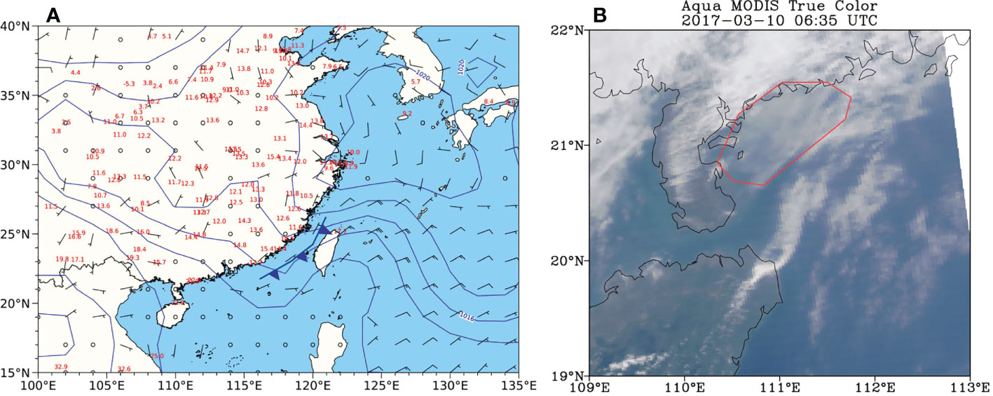
Figure 1 SLP (contour), wind (barb), and temperature (number) at 2000BJT on March 10th, 2017 (A), and the MODIS infrared true color at 1435BJT on March 10th, 2017 (B).

3.2 Offshore and onshore observations

The air temperature, humidity, wind speed, and fog duration at the offshore station (point A in Figure 3; 110.86°E, 21.02°N) from 1200BJT on March 10th to 1200BJT on March 11th, 2017 are displayed inFigure 2A. According to Kunkel (1984), the fog extinction coefficient is correlated with LWC: a horizontal visibility of less than 1 km suggests LWC is greater than 0.018 g/m³ at a height of 5 m and 0.027 g/m³ at a height of 30 m. Hence, in our study, according to the principle of linear interpolation, an LWC greater than 0.02 g/m³ at 10 m was considered as a sign of sea fog. As suggested by the observed LWC time series, sea fog took place rapidly and formed after 21:00 on March 10th, and lasted until 06:00 on March 11th (marked as a shaded area in Figure 2A). The 10 m air temperature had an obvious decline from before sea fog formation to the first hour after its formation, then slightly increased in the subsequent fog evolution process, and dropped after the fog dissipated. The humidity rose before and during the sea fog event.

FIGURE 2

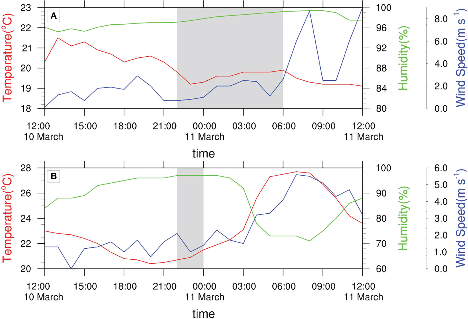
Figure 2 Time series of wind speed, air temperature, humidity, and fog duration (gray shaded areas) for station (A) and station (B) in Figure 3.

Figure 2B shows the 2 m air temperature, 2 m humidity, 10 m wind speed, and fog duration at the onshore Xuwen observation station (point B in Figure 3; 110.18°E, 20.33°N) from 1200BJT on March 10th to 1200BJT on March 11th, 2017. Although sea fog is defined as a weather event in which a large number of water droplets or ice crystals are suspended in the atmospheric boundary layer and cause atmospheric visibility at sea (including on shores and islands) to drop below 1 km (Wang, 1985), the visibility threshold for fog formation at the onshore station was set at 1100 m (fog occurred in the prior hour) or 900 m (no fog occurred in the prior hour) in this study, as the Belfort Model 6000 Visibility Sensor may have an error of ±10%. The duration of onshore sea fog was approximately two hours from 22:00 to 24:00 on March 10th (marked as the shaded area in Figure 2B), which was shorter than the duration of offshore sea fog. The wind speed increased before sea fog formation, favoring the transport of moisture from the sea to the onshore station, which resulted in slight increases in humidity and sea fog formation.

FIGURE 3

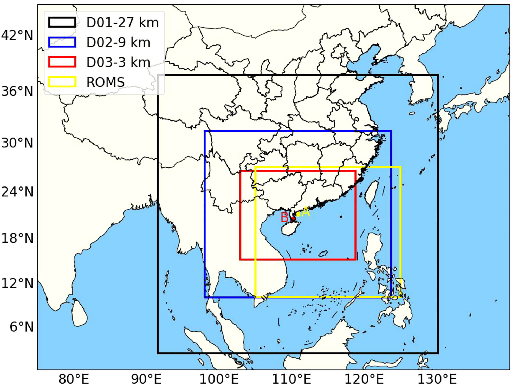
Figure 3 Simulation domains of the models (black, blue, and red boxes are the simulation domains of the three-layer atmospheric model, the yellow box is the simulation domain of the oceanic model, and the stations marked by A and B are the offshore and onshore observation stations, respectively).

3.3 Model experimental design

With one offshore observation station (110.86°E, 21.02°N) at the center, the atmospheric model consisted of three nested layers with spatial resolutions of 3, 9, and 27 km, respectively. The coupled Regional Ocean Model System (ROMS) model was composed of the WRF model’s innermost oceanic layer and the land to the west (the yellow frame in Figure 3). To improve the vertical resolution of the near-surface layer, the atmospheric model was divided into 66 layers, and the ocean model 40 layers. Major parameterization schemes for the atmospheric model were as follows: MYNN2.5 (Sukoriansky et al., 2005) for the boundary layer; New Thompson (Thompson et al., 2008) as the microphysical scheme; RRTM (Mlawer et al., 1997) for longwave radiation; Dudhia (Dudhia, 1989) for shortwave radiation; Noah (Chen and Dudhia, 2001) for the land surface process; New Kain-Fritsch (Kain, 2004) for the outer layer of cumulus but no scheme for the innermost layer, and the Monin-Obukhov scheme (Zhang and Anthes, 1982) for the near-surface layer (Table 1). Gridpoint Statistical Interpolation was used in the atmospheric model of both the coupled and uncoupled models for cyclic assimilation every 6 h. The assimilated data were regular Global Telecommunication System (GTS) observations of the ground and automatic stations. ERA5 reanalysis data were used in the WRF model as the initial field and boundary condition driver with a horizontal resolution of 0.25°, 37 vertical layers, and a temporal resolution of 6 h. The hindcasts data in the HYCOM model were used in the ROMS model as the initial field and boundary condition driver with a horizontal resolution of 0.08°, 40 vertical layers, and a temporal resolution of 24 h.

TABLE 1

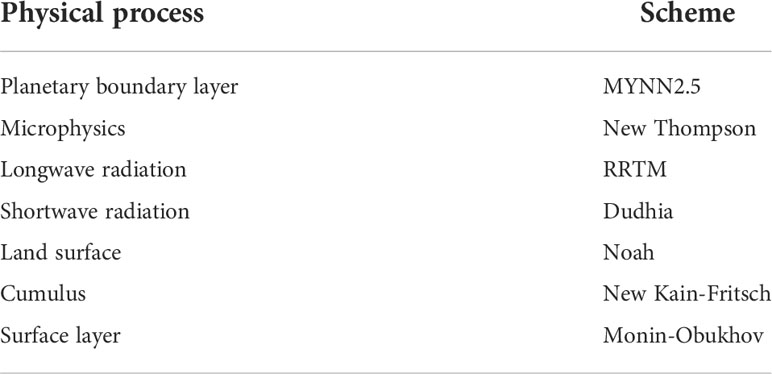
Table 1 Major parameterization schemes.

4 Results of model simulation

4.1 Model validation and analysis

MICAPS data and observation data of sea and offshore stations are used to validate the model results in this section.

4.1.1 Spatiotemporal distribution of root-mean-square error

To interpret the deviation of model data from the measured MICAPS data for the innermost zone (3 km, D03), the root-mean-square error (RMSE) spatiotemporal distributions of the 2 m air temperature and 10 m wind speed were constructed. According to the RMSE spatial distribution of 2 m air temperature in the northwest of the South China Sea (Figures 4A, B), the coupled model RMSE was lower than that of the uncoupled model on both sides of the Qiongzhou Strait, while the uncoupled model RMSE was smaller in the Pearl River Delta region. The 2 m air-temperature RMSE (Figure 4C) of the coupled model was lower than that of the uncoupled model, yet they had the same trend; both models reached a maximal RMSE during 1400BJT to 1700BJT (Beijing time) on March 10th, but the uncoupled model RMSE was approximately 1.6 times that of the coupled model at this time.

FIGURE 4

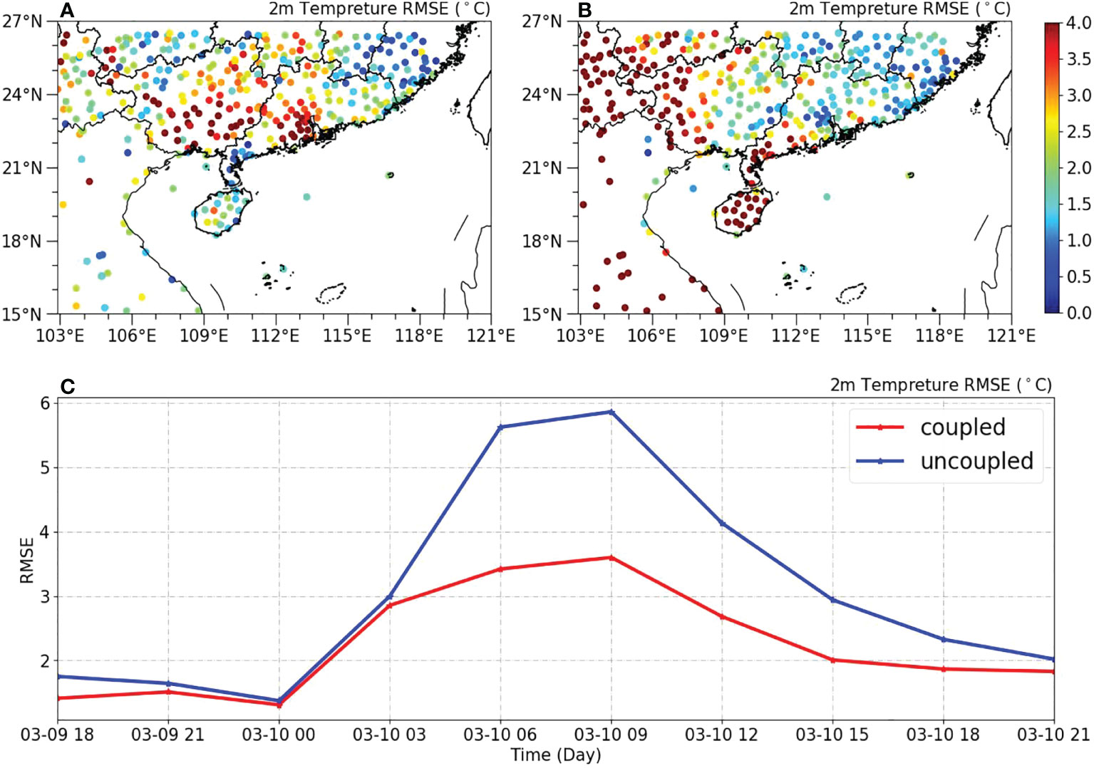
Figure 4 Spatial distribution of 2 m air temperature RMSE for (A) the coupled model and (B) the uncoupled model) and (C) time series.

The RMSE spatial distribution of the 10 m wind speed for the coupled model (Figure 5A) was consistent with that of the uncoupled model (Figure 5B), and the maximum RMSE errors for both models were present near the northwest boundary of the simulated area. The RMSE in the coastal area was mostly below 2 m/s for both models. According to the RMSE time series (Figure 5C), after 1400BJT on March 10th, the RMSE of the two models followed the same trend, yet the coupled model had a slightly larger RMSE. The maximum wind speed RMSE difference between the two models was below 0.6 m/s in the studied period.

FIGURE 5

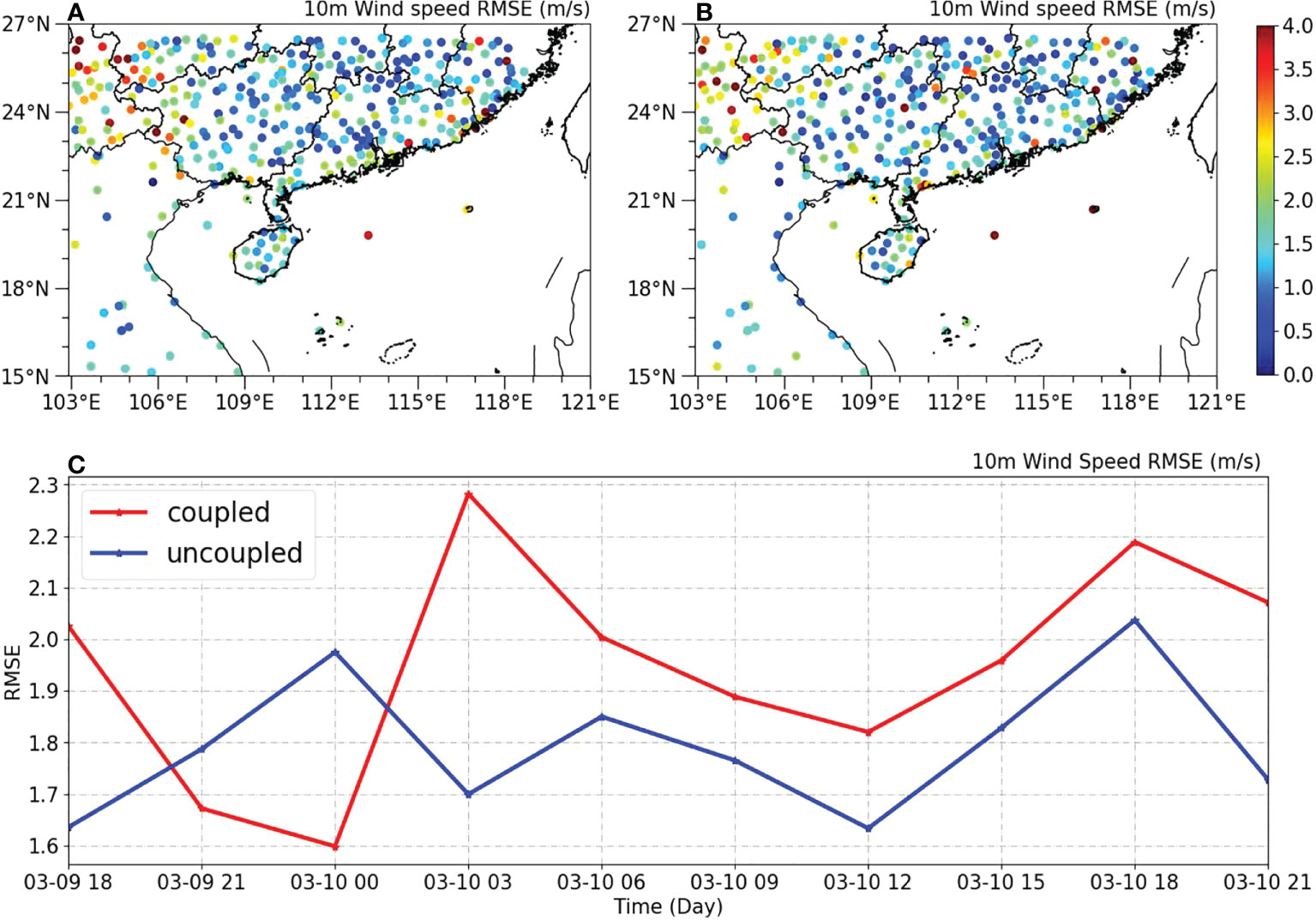
Figure 5 Spatial distribution of 10 m wind speed RMSE for (A) the coupled model and (B) the uncoupled model and (C) time series.

4.1.2 Sea fog simulation compared with offshore and onshore observation

The air temperature, humidity, wind speed, and fog duration observed at the offshore station (110.86°E, 21.02°N) and onshore Xuwen observation station (110.18°E, 20.33°N) were used to confirm the simulation results of the coupled and uncoupled models (Figures 2 and 6). Compared with the offshore station (Figure 2A), the 2 m temperature from the coupled model (Figure 6A) had a similar trend, while that from the uncoupled model was clearly different. The humidity of the coupled model (Figure 6B) reached 100% during the sea fog event, while the that from of the uncoupled model decreased, different from the trend seen in the observations. For simulation results and observations, increasing wind speed led to fog dissipation. The fog in the coupled model dissipated one hour later than that in the observations, which was related to observed light rain, while dissipation in the uncoupled model was one hour earlier, and a fog forecast from 0800BJT to 1100BJT on March 11th was lacking.

FIGURE 6

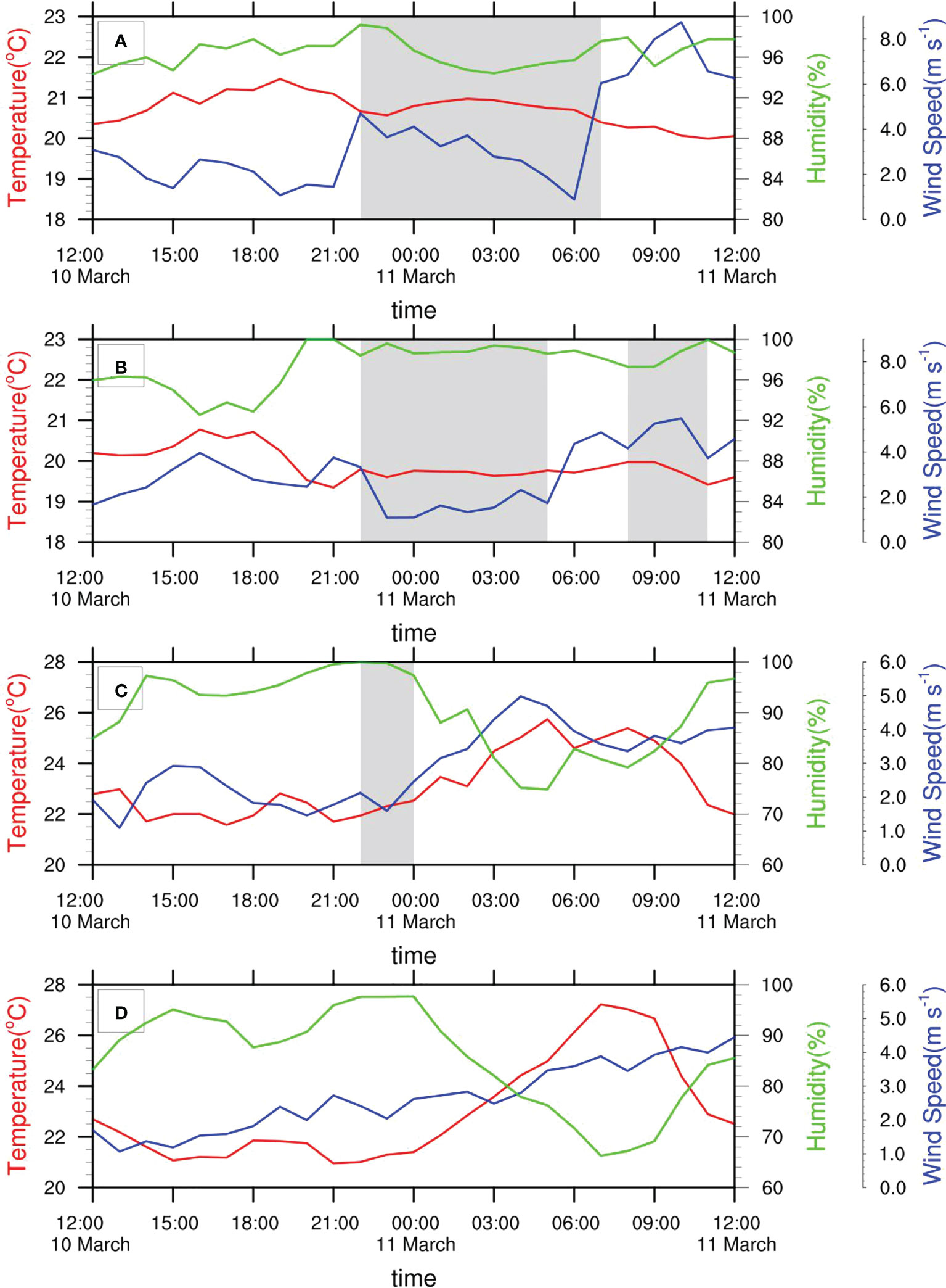
Figure 6 Time series of wind speed, air temperature, humidity, and fog duration (gray shaded areas) at station A [(A) for the coupled model; (B) for the uncoupled model] and station B (C) for the coupled model; (D) for the uncoupled model.

The 2 m air temperature, 2 m humidity, 10 m wind speed, and fog duration at the onshore Xuwen observation station (Figure 2B) were used to further check the simulation results of the coupled and uncoupled models (Figures 6C, D). Unlike the different heights adopted in the observation and simulation during the offshore phase, the height for the simulation was the same as that for observation at the land station, which brought the coupled and uncoupled model output trends closer to observations before and after the fog. For fog evolution, the coupled-model (Figure 6C) fog duration output was consistent with the observed duration, while no fog was forecasted by the uncoupled model (Figure 6D), most likely resulting from the stronger simulated wind and lower humidity.

The coupled model had lower 2 m air temperature RMSE than the uncoupled model, compared with MICAPS data (Figure 4). In addition, the coupled model simulated the duration of the sea fog closer to offshore observations, while the sea fog dissipated one hour earlier and a false fog event was occurred in the uncoupled model (Figures 2A,6A, B). The comparison with the measured visibility observed at the onshore Xuwen station (Figure 2B) showed that the coupled model forecasted fog duration more precisely, and the uncoupled model failed to forecast a fog event. Those results indicated that the coupled model simulated the sea fog better than the uncoupled model.

4.2 Effects of air–sea interaction

Taking LWC>0.02 g·m^-3 as the threshold for fog formation, according to the coupled and uncoupled model simulations, the fog moved from the coast of Western Guangdong to the Qiongzhou Strait on March 11th (not shown). According to spatial distribution of LWC at the lowest model level from the coupled and uncoupled models at 0700BJT on March 11th (Figure 7), the fog was smaller in area and weaker in the uncoupled model than in the coupled model. Within the target area marked by the black rectangular frame in Figure 7, a large area of strong fog was forecasted by the coupled model, while no fog was forecasted by the uncoupled model. The coupled and uncoupled model outputs differed for the areas east and west of the target area, but the difference was not obvious at other times.

FIGURE 7

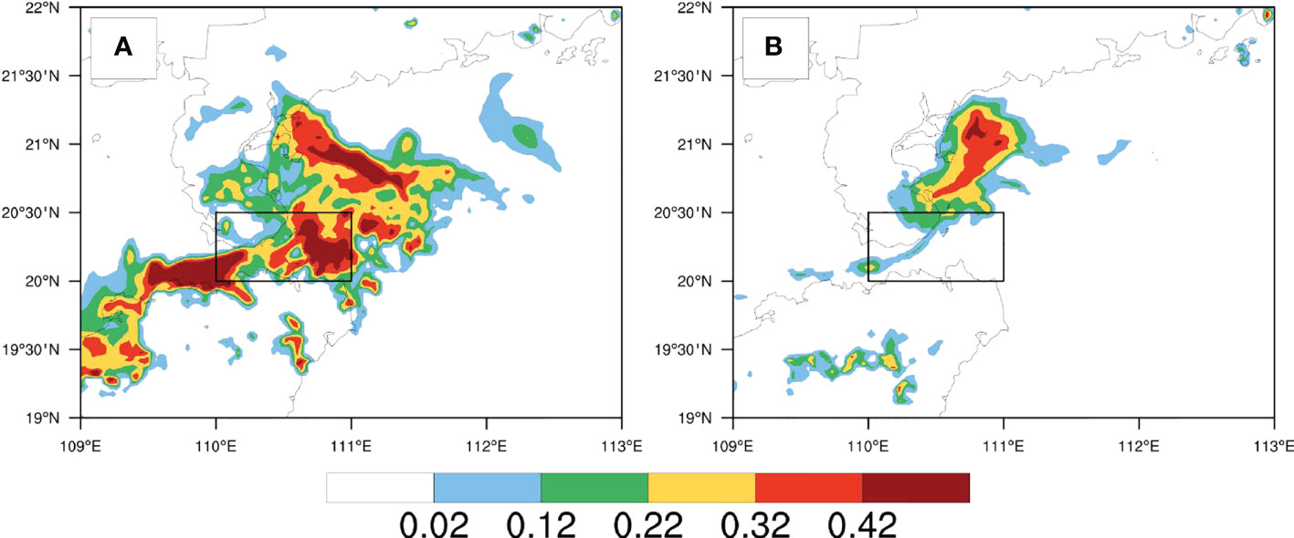
Figure 7 Spatial distribution of LWC (g·m^-3) at the lowest model level at 0700BJT on March 11th, 2017 as forecasted by (A) the coupled model and (B) the uncoupled model.

To clarify the different results in terms of fog area and intensity in the target area, the coupled and uncoupled model simulation results were compared and the sea–air interactions analyzed. The maximum LWC exceeded 0.42 g·m^-3 at 0700BJT on March 11th, and the average LWC might have been greater than 0.02 g·m^-3 for the uncoupled model, as there were a few scattered large-LWC-value zones in the target area (Figure 7). Therefore, when judging whether fog forms in the target area, the size of the fog area should also be considered. Against the criterion that fog forms when the LWC of three-fourths of the target area exceeds the threshold of 0.02 g·m^-3, no fog formed in the uncoupled model, while fog lasted from 0300BJT to 0800BJT on March 11th in the coupled model (the gray shaded area in Figure 8A).

FIGURE 8

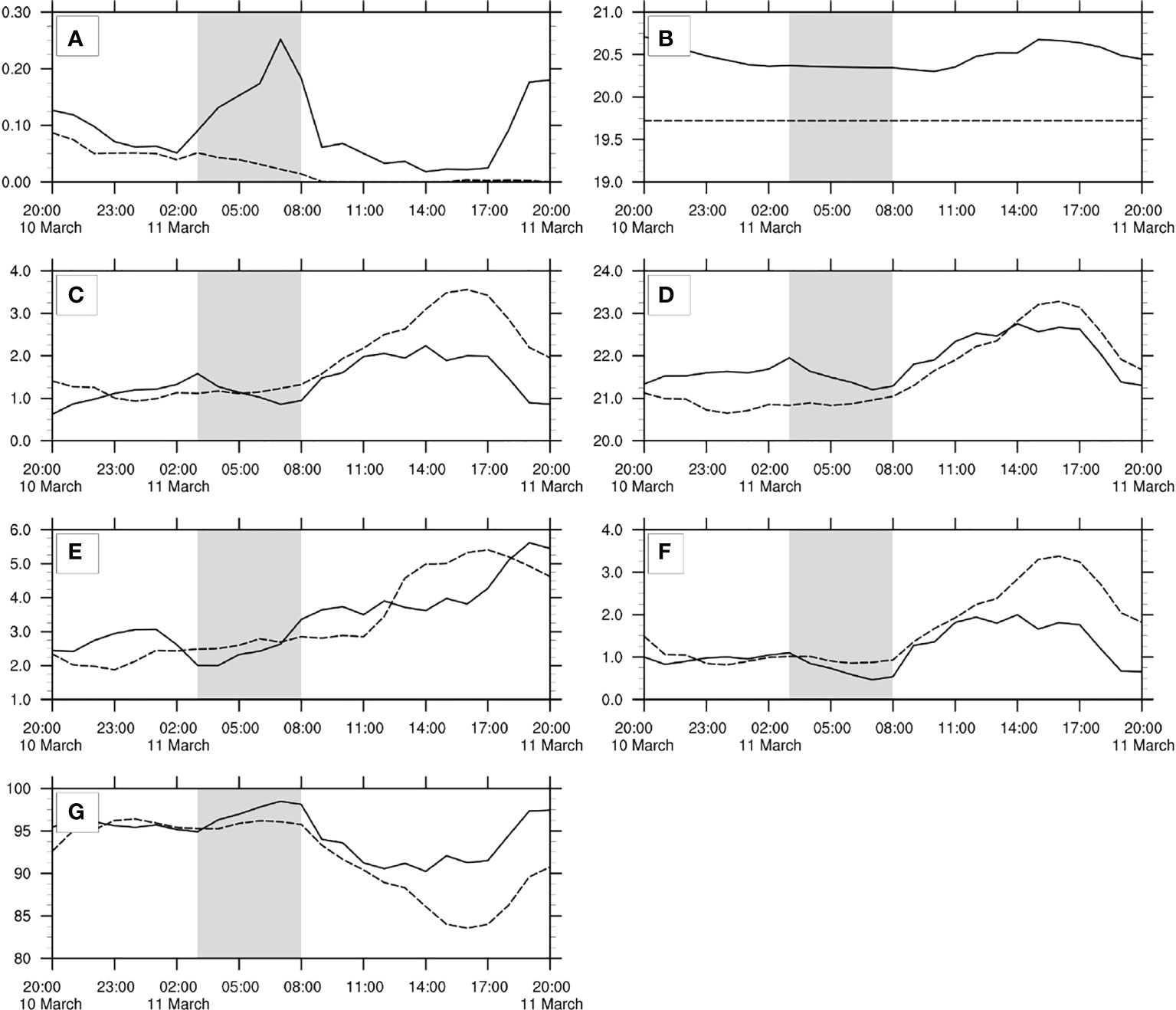
Figure 8 Temporal evolution of (A) LWC (g·m^-3), (B) SST (℃), (C) ASTD (℃), (D) 2 m air temperature (℃), (E) wind speed (m·s^-1), (F) ADTD (℃), and (G) 2 m relative humidity (%) average value over the target area (marked by the black rectangular frame in Figure 7) by using the coupled (solid line) and uncoupled (dashed line) models.

SST average value over the target area (marked by the black rectangular frame in Figure 7) in the coupled model was slightly higher than that in the uncoupled model with constant SST, but it clearly decreased before fog formation (Figure 8B). LWC showed the opposite trend to ASTD in the coupled model (Figure 8C), and the shift in LWC was one hour earlier than that of ASTD, which was most likely due to LWC being an average value for the entire area (given fog does not form simultaneously in an area). The change of ASTD was small during pre-fog and fog processes in the uncoupled model, and the fog simulation failed. The influence of ASTD on fog evolution should be analyzed by three factors. Firstly, the low-level atmosphere was cooled by cold water prior to fog formation, which reduced the 2 m temperature of the fog process and promoted the condensation of water vapor at low levels (Figure 8D). Secondly, wind speed in the coupled model decreased significantly before fog formation and was weaker than in the uncoupled model during fog evolution (Figure 8E), suggesting that decreasing ASTD made the low-level stratification more stable and reduced low-level wind speed. However, wind speed in the coupled model exceeded that in the uncoupled model after 0700BJT, corresponding to fog dissipation. Finally, the 2 m air temperature decreased during fog evolution and caused a significant decrease in air-dew point temperature difference (ADTD) (Figure 8F). Because a smaller ADTD can cause higher humidity, this led to an increase in 2 m humidity during fog evolution (Figure 8G). In general, ASTD affects the evolution of sea fog by lowering the temperature, increasing the humidity, and strengthening the low-level atmospheric stable stratification.

Equations (1) and (2) are empirical equations for sensible and latent heat fluxes, respectively:

$\begin{array}{ll}SHF=\rho C_p{c}_{h}U\left(T_s-T_a\right)& (1)\end{array}$

$\begin{array}{ll}\text{LHF }=\rho {\text{L}}_{\text{e}}{c}_{e}U\left(q_s-q_a\right)& (2)\end{array}$

where ρ is the density of air; L_e is the latent heat of evaporation for water; C_p is the specific heat of air at constant pressure; c_e and c_h are the water vapor transfer coefficient and heat exchange coefficient, respectively, U is the mean wind speed at a. height of 10 m; T_s and T_a are the potential temperatures of air at the sea surface and near-surface atmosphere, respectively; and q_s and q_a are the specific humidity of air at the sea surface and near-surface atmosphere, respectively (Yu and Weller, 2007).

From the difference of sensible heat flux and latent heat flux average value over the target area (marked by the black rectangular frame in Figure 7) between the coupled and non-coupled models, the main characteristics of the influence of air–sea interaction on sea fog are the negative sensible heat flux before fog and the negative latent heat flux during fog (Figure 9). The decrease of SST before fog cools the atmosphere through sensible heat flux exchange. Latent heat flux in the coupled model was negative at the beginning of fog formation. In the empirical equation for latent heat flux, q_s and q_a are the specific humidity of the sea surface and near-surface atmosphere, respectively, so when the latent heat flux is negative, it means that q_s is smaller than q_a, which indicates condensation caused by oversaturation. The negative latent heat flux at the beginning of fog for the coupled model was related to the drop in SST prior to fog formation, as well as the drop in 2 m air temperature during fog evolution that led to condensation and stable stratification in the near-surface area. Therefore, advective fog formation and evolution depend not only on SST cooling the atmosphere through sensible heat flux exchange, but also on the effect of the negative latent heat flux during the condensation of advective moist air.

FIGURE 9

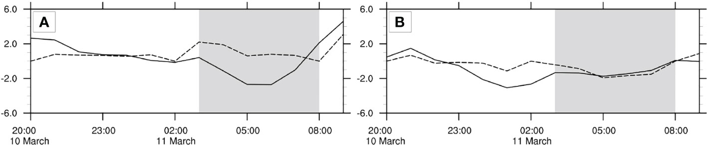
Figure 9 Temporal evolution of (A) latent heat flux (W·m^-2) and (B) sensible heat flux (W·m^-2) average value over the target area (marked by the black rectangular frame in Figure 7) by using the coupled (solid line) and uncoupled (dashed line) models.

To confirm the effect of the decrease in ASTD, Figure 10 shows the vertical-time profiles of air temperature, horizontal wind speed, and relative humidity average value over the target area (marked by the black rectangular frame in Figure 7). Corresponding to extremely low SST in the uncoupled model (Figure 8B), the temperature profiles between the two simulations suggest that the temperature in the uncoupled simulation is noticeably lower than that in the coupled simulation (Figure 10A). Due to the exchange of heat flux caused by the SST decline of the coupled model, there is an obvious inversion layer below 200 m before and at the beginning of fog, which increases the stability of the low layer and limits the mixing with the upper air. The horizontal wind speed on the sea surface before fog formation in the coupled mode is significantly lower than that at a height of 200 m, so the air–sea interaction leads to the decrease of sea surface wind and the increase of upper wind speed (Figure 10B). The decrease of low-level temperature after fog formation promoted the condensation of water vapor (Figure 10C), while the decrease of wind vertical shear led to the thickening of the humidity layer. In the dissipation stage, the increase of wind speed led to the decrease of low-level humidity. In contrast, the SST in the uncoupled model remained unchanged, and air temperature was mainly affected by diurnal variation. Therefore, there was a weaker inversion layer (Figure 10D), stronger vertical mixing (Figure 10E), and lower humidity (Figure 10F) in the uncoupled model.

FIGURE 10

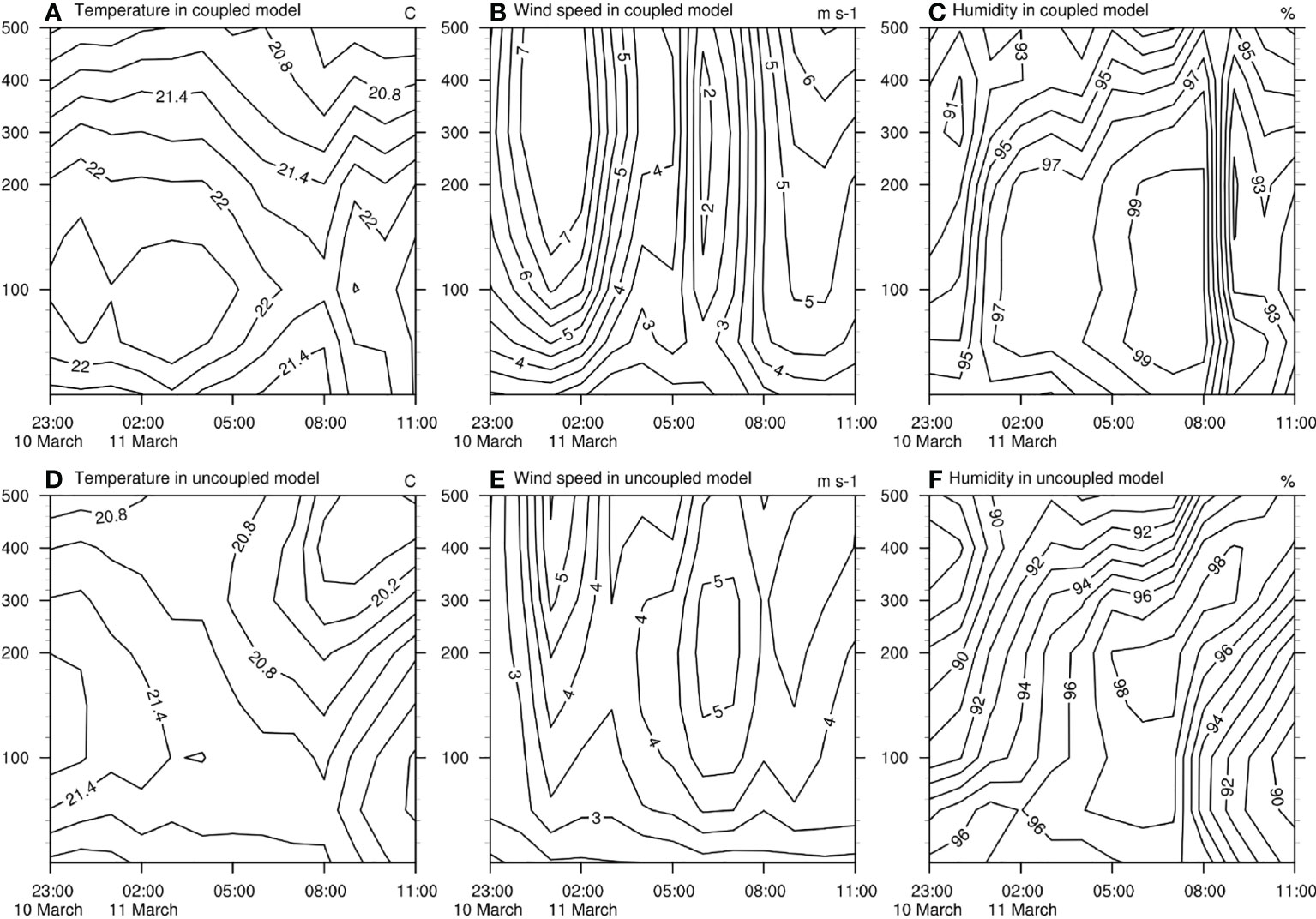
Figure 10 Vertical time profiles of (A) air temperature (℃), (B) horizontal wind speed (m·s^-1), and (C) relative humidity (%) average value over the target area (marked by the black rectangular frame in Figure 7) at 0200BJT (black), 0500BJT (green), and 0900BJT (red) for the coupled model. (D–F) same as (A–C), but for the uncoupled model.

The sea–air interactions impacting on sea fog were investigated by comparing the differences of SST, ASTD, sensible and latent heat fluxes, wind and temperature between coupled and uncoupled model simulation results in terms of fog area and intensity in the target area. In the coupled model, the decrease of SST before fog formation (Figure 8A) cooled the low-level temperature (Figure 8D) through the negative sensible heat flux (Figure 9B) and increased the low-level humidity (Figure 8G) through negative latent heat flux (Figure 9A). These exchanges of sensible and latent heat fluxes resulted in an obvious inversion layer below 200 m (Figure 10A) before and at the beginning of the fog, which increased low-level stability, and limited mixing with upper air (Figure 10B). These processes of forming fog failed in the uncoupled model. Those results indicated that the processes of cooling, humidification, and strong low-level stability impacted by air–sea interaction had important influences on the formation and evolution of sea fog.

5 Conclusion and discussion

Ocean-atmosphere coupled and uncoupled models were used to simulate one sea fog event. Unlike the constant SST in the uncoupled model, SST in the coupled model was updated at preset times, thus realizing the exchange of momentum and heat between the ocean and the atmosphere. Since sea fog is caused due to complex interactions between atmospheric and oceanic environments (Yun and Ha, 2022), this study investigated the effects of air–sea interactions on the formation, evolution, and dissipation of sea fog.

Against MICAPS data, the 2 m air temperature RMSE of the coupled model was lower than that of the uncoupled model, but the 10 m wind speed RMSE of the two models was similar. Sea fog duration in the coupled model was closer to offshore observations, but fog dissipated one hour earlier in the uncoupled model, and another fog event was reported afterwards, which was an error because fog was not actually observed. For onshore simulations, the coupled model forecasted fog duration more precisely, but the uncoupled model failed to forecast a fog event that, according to measured visibility, was observed at the onshore Xuwen station.

For the results of the coupled model, the air–sea interaction mainly affected the formation and evolution of sea fog through cooling, humidification, and strengthening the lower atmospheric stable stratification. The SST decreased before fog formation, cooling the low-level temperature through the negative sensible heat flux exchange and increasing the low-level humidity through negative latent heat flux exchange. These exchanges of sensible and latent heat fluxes at the air–sea interface before and at the beginning of the fog resulted in an obvious inversion layer below 200 m, increased low-level stability, and limited mixing with upper air. These processes of forming fog failed in the uncoupled model. In the fog dissipation stage, the enhancement of vertical mixing and the increase of low-level wind speed made the low-level humidity decrease.

Sea fog is an important weather phenomenon in the South China Sea because of its industrial impacts on ocean traffic, coastal ecosystems, and the energy balance of the climate system (Clement et al., 2009; Oliphant et al., 2021). Sea fog is not only affected by surface features but is also sensitive to aerosol characteristics (LaDochy, 2005; Boutle et al., 2018). Guangdong Province near the South China Sea is one of China’s well-developed industrial regions, with associated large quantities of aerosol emissions. Importantly, aerosols are the key to fog water nucleation. Therefore, numerical simulations including chemical components are also worthy of further study in the future.

Data availability statement

The original contributions presented in the study are included in the article/supplementary material. Further inquiries can be directed to the corresponding authors.

Author contributions

Conceptualization: LH, SZ, and FX; method: LH, FX, JL, and JX; software: LH, SZ, and ZL; data curation: LH, GY, and SC; writing—original draft preparation: LH, FX, and SZ; writing—review and editing: LH, FX, JL, and JX; visualization: LH, GY, SC, and JD; all authors contributed to the article and approved the submitted version.

Funding

The study was supported by the Key Area R&D Program of Guangdong Province, China (Grant no. 2020B0101130021), Guangxi Key Research and Development Program (Grant no. AB20159013), the National Key R&D Program of China (Grant no. 2018YFA0605604), the Strategic Priority Research Program of Chinese Academy of Sciences (Grant no. XDA20060503), and the National Natural Science Foundation of China (Grant nos. 41675136 and 41875170).

Conflict of interest

The authors declare that the research was conducted in the absence of any commercial or financial relationships that could be construed as a potential conflict of interest.

Publisher’s note

All claims expressed in this article are solely those of the authors and do not necessarily represent those of their affiliated organizations, or those of the publisher, the editors and the reviewers. Any product that may be evaluated in this article, or claim that may be made by its manufacturer, is not guaranteed or endorsed by the publisher.

References

Barker E. H. (1977). A maritime boundary-layer model for the prediction of fog. Boundary-Layer Meteorology. 11 (3), 267–294.

Google Scholar

Boutle I., Price J., Kudzotsa I., Kokkola H., Romakkaniemi S. (2018). Aerosol–fog interaction and the transition to well-mixed radiation fog. Atmos. Chem. Phys. 18 (11), 7827–7840.

Google Scholar

Carniel S., Barbariol F., Benetazzo A., Bonaldo D., Falcieri F. M., Miglietta M. M., et al. (2016). Scratching beneath the surface while coupling atmosphere, ocean and waves: analysis of a dense water formation event. Ocean. Modeling. 101, 101–112.

Google Scholar

Chen F., Dudhia J. (2001). Coupling an advanced land surface-hydrology model with the Penn state–NCAR MM5 modeling system. part I: Model implementation and sensitivity. Monthly. weather. Rev. 129 (4), 569–585.

Google Scholar

Clement A. C., Burgman R., Norris J. R. (2009). Observational and model evidence for positive low-level cloud feedback. Science 325, 460–464.

PubMed Abstract | Google Scholar

Dudhia J. (1989). Numerical study of convection observed during the winter monsoon experiment using a mesoscale two-dimensional model. J. Atmospheric. Sci. 46 (20), 3077–3107.

Google Scholar

Fisher E. L., Caplan P. (1963). An experiment in numerical prediction of fog and stratus. J. Atmospheric. Sci. 20 (5), 425–437.

Google Scholar

Fu G., Wang J. Q., Zhang M. G., Guo J. T., Guo M. K., G K. C. (2004). An observational and numerical study of a sea fog event over the yellow Sea on 11 apri. Peiodical. Ocean. Univ. China 34 (05), 720–726. doi: 10.16441/j.cnki.hdxb.2004.05.006(in Chinese

CrossRef Full Text | Google Scholar

Gao S. H., Qi Y. L., Zhang S. B., Fu G. (2010). Initial conditions improvement of Sea fog numerical modeling over the yellow Sea by using cycling 3DVAR part I :WRF numerical experiments. Peiodical. Ocean. Univ. China 40 (10), 1–9. doi: 10.16441/j.cnki.hdxb.2010.10.001(in Chinese

CrossRef Full Text | Google Scholar

Gultepe I., Milbrandt J. A. (2007). Microphysical observations and mesoscale model simulation of a warm fog case during FRAM project. Pure. Appl. Geophysics. 164 (6), 1161–1178. doi: 10.1007/s00024-007-0212-9

CrossRef Full Text | Google Scholar

Han L. G., Long J. C., Xu F., Xu J. J. (2022). Decadal shift in sea fog frequency over the northern south China Sea in spring: Interdecadal variation and impact of the pacific decadal oscillation. Atmospheric. Res. 265. doi: 10.1016/j.atmosres.2021.105905

CrossRef Full Text | Google Scholar

Heo K. Y., Ha K. J. (2010). A coupled model study on the formation and dissipation of sea fogs. Monthly. Weather. Rev. 138 (4), 1186–1205. doi: 10.1175/2009MWR3100.1

CrossRef Full Text | Google Scholar

Huang H. J., Liu H. N., Huang J., Mao W. K., Bi X. Y. (2015). Atmospheric boundary layer structure and turbulence during Sea fog on the southern China coast. Monthly. Weather. Rev. 143 (5), 1907–1923. doi: 10.1175/MWR-D-14-00207.1

CrossRef Full Text | Google Scholar

Huang H. J., Zhan G. W., Liu C. X., Tu J., Mao W. K. (2016). A case study of numerical simulation of sea fog on the southern China coast. J. Trop. Meteorology. 22 (4), 497–507. doi: 10.16555/j.1006-8775.2016.04.005

CrossRef Full Text | Google Scholar

Huang Y., Peng X. ,. D. (2017). The impact of an improved planetary boundary layer parameterization scheme on the simulation of fog. Chin. J. Atmospheric. Sci. 41 (03), 533–543. doi: 10.3878/j.issn.1006-9895.1606.16152(in Chinese

CrossRef Full Text | Google Scholar

Hu R. J., Zhou F. X. (1997). A numerical study on the effect of air-sea conditions on the process of seafog. J. Ocean. Univ. Qingdao. 27 (03), 16–24.

Google Scholar

Kain J. S. (2004). The kain-fritsch convective parameterization: an update. J. Appl. meteorology. 43 (1), 170–181.

Google Scholar

Kim C. K., Yum S. S. (2010). Local meteorological and synoptic characteristics of fogs formed over incheon international airport in the west coast of Korea. Adv. Atmospheric. Sci. 27 (4), 761–776. doi: 10.1007/s00376-009-9090-7

CrossRef Full Text | Google Scholar

Kim C. K., Yum S. S. (2012). A numerical study of sea-fog formation over cold sea surface using a one-dimensional turbulence model coupled with the weather research and forecasting model. Boundary-Layer Meteorology. 143 (3), 481–505. doi: 10.1007/s10546-012-9706-9

CrossRef Full Text | Google Scholar

Koračin D., Businger J. A., Dorman C. E., Lewis J. M. (2005). Formation, evolution, and dissipation of coastal sea fog. Boundary-Layer Meteorology. 117 (3), 447–478. doi: 10.1007/s10546-005-2772-5

CrossRef Full Text | Google Scholar

Koračin D., Dorman C. E. (2017). Marine fog: Challenges and advancements in observations, modeling, and forecasting (Berlin: Springer), 540.

Google Scholar

Koračin D., Lewis J., Thompson W. T., Dorman C. E., Businger J. A. (2001). Transition of stratus into fog along the California coast: Observations and modeling. J. Atmospheric. Sci. 58 (13), 1714–1731.

Google Scholar

Kumar V. S., Nair A. M. (2016). Inter-annual variations in wave spectral characteristics at a location off the central west coast of India. Ann. Geophys. 33, 159–167. doi: 10.5194/angeo-33-159-2015

CrossRef Full Text | Google Scholar

Kumar R. P., Vimlesh P. (2016). Upper oceanic response to tropical cyclone phailin in the bay of bengal using a coupled atmosphere-ocean model. Ocean. Dynamics 67 (1), 51–64.

Google Scholar

LaDochy S. (2005). The disappearance of dense fog in Los Angeles: another urban impact? Phys. Geogr. 26 (3), 177–191.

Google Scholar

Mlawer E. J., Taubman S. J., Brown P. D., Iacono M. J., Clough. S. A. (1997). Radiative transfer for inhomogeneous atmospheres: RRTM, a validated correlated-k model for the longwave. J. Geophysical. Research.: Atmospheres. 102 (D14), 16663–16682. doi: 10.1029/97jd00237

CrossRef Full Text | Google Scholar

Nakanishi M. (2000). Large-Eddy simulation of radiation fog. Boundary-layer. meteorology. 94 (3), 461–493.

Google Scholar

O’Brien T. A., Sloan L. A., Chuang P. Y., Faloona I. C., Johnstone J. A. (2013). Multidecadal simulation of coastal fog with a regional climate model. Climate Dynamics. 40 (11-12), 2801–2812. doi: 10.1007/s00382-012-1486-x

CrossRef Full Text | Google Scholar

Olabarrieta M., Warner J. C., Armstrong B., He R., Zambon J. B. (2012). Ocean–atmosphere dynamics during hurricane Ida and Nor’Ida: an application of the coupled ocean–atmosphere-wave-sediment transport (COAWST) modeling system. Ocean. Model. 43-44, 112–137. doi: 10.1029/2011JC007387

CrossRef Full Text | Google Scholar

Olabarrieta M., Warner J. C., Kumar N. (2011). Wave-current interaction in willapa bay. J. Geophys. Res. 116, C12014. doi: 10.1029/2011JC007387

CrossRef Full Text | Google Scholar

Oliphant A. J., Baguskas S. A., Fernandez D. M. (2021). Impacts of low cloud and fog on surface radiation fluxes for ecosystems in coastal California. Theor. Appl. Climatol. 144 (1), 239–252.

Google Scholar

Oliver D. A., Lewellen W. S., Williamson G. G. (1978). The interaction between turbulent and radiative transport in the development of fog and low-level stratus. J. Atmospheric. Sci. 35 (2), 301–316.

Google Scholar

Qu F. Q., Liu S. D., Yi Y. M., Huang J. (2008). The observation and analysis of a Sea fog event in south China Sea. J. Trop. Meteorology. 24 (5), 490–496. doi: 10.3724/SP.J.104,7.2008.00014/

CrossRef Full Text | Google Scholar

Rao L. J., Gao S. ,. H., Zhang K. (2019). Impact of boundary layer and cloud microphysics schemes in WRF model on numerical simulation of two yellow Sea fog cases. Adv. Meteorological. Sci. Technol. 9 (06), 12–19. doi: 10.3969/j.issn.2095-1973.2019.06.002(in Chinese

CrossRef Full Text | Google Scholar

Ricchi A., Miglietta M. M., Falco P. P., Bergamasco A., Benetazzo A., Bonaldo D., et al. (2016). On the use of a coupled ocean-atmosphere-wave model during an extreme cold air outbreak over the Adriatic Sea. Atmos. Res. 172–173, 48–85. doi: 10.1016/j.atmosres.2015.12.023

CrossRef Full Text | Google Scholar

Skyllingstad E. D., Vickers D., Mahrt L., Samelson R. (2007). Effects of mesoscale sea-surface temperature fronts on the marine atmospheric boundary layer. Boundary-Layer Meteorology. 123 (2), 219–237. doi: 10.1007/s10546-006-9127-8

CrossRef Full Text | Google Scholar

Sukoriansky S., Galperin B., Perov V. (2005). Application of a new spectral theory of stably stratified turbulence to the atmospheric boundary layer over sea ice. Boundary-layer. meteorology. 117 (2), 231–257. doi: 10.1007/s10546-004-6848-4

CrossRef Full Text | Google Scholar

Thompson G., Field P. R., Rasmussen R. M., Hall W. D. (2008). Explicit forecasts of winter precipitation using an improved bulk microphysics scheme. Part II: Implementation of a new snow parameterization. Monthly. Weather. Rev. 136 (12), 5095–5115. doi: 10.1175/20,08MWR2387.1

CrossRef Full Text | Google Scholar

Tokinaga H., Xie S. P. (2009). Ocean tidal cooling effect on summer sea fog over the Okhotsk Sea. J. Geophysical. Res. Atmospheres. 114, D104102. doi: 10.1029/2008JD011477

CrossRef Full Text | Google Scholar

Wang B. H. (1985) (Sea fog.China Ocean Press), 330.

Google Scholar

Wang B. (2015). “Comparison of the aerosol effect in the numerical simulation of sea fog and land fog,” in Master thesis(Ocean University of China (in Chinese).

Google Scholar

Wang Y. M., Gao S. H., Sun J. L., Zhang S. P. (2012). Assimilating MTSAT-derived humidity in nowcasting Sea fog over the yellow Sea. Weather. Forecasting. 29 (2), 205–225. doi: 10.1175/WAF-D-12-00123.1

CrossRef Full Text | Google Scholar

Warner J. C., Armstrong B., He R., Zambon J. B. (2010). Development of a coupled ocean–atmosphere–wave–sediment transport (coawst) modeling system. Ocean. Model. 35 (3), 230–244.

Google Scholar

Yang Y., Gao S. H. (2016). Sensitivity study of vertical resolution in WRF numerical simulation for sea fog over the yellow sea. Acta Meteorologica. Sin. 74 (06), 974–988. doi: 10.11676/qxxb2016.062(in Chinese

CrossRef Full Text | Google Scholar

Yan S. Q., Zhu B., Huang Y., Zhu J., Kang H. Q., Lu W., et al. (2020). To what extents do urbanization and air pollution affect fog? Atmospheric. Chem. Phys. 20, 5559–5572.

Google Scholar

Yan S. Q., Zhu B., Zhu T., Shi C. E., Liu D. Y., Kang H. Q., et al. (2021). The effect of aerosols on fog lifetime: observational evidence and model simulations. Geophysical. Res. Lett. 48 (2), e2020GL61803. doi: 10.1029/2020GL091156

CrossRef Full Text | Google Scholar

Yun J., Ha K. J. (2022). Physical processes in Sea fog formation and characteristics of turbulent air-Sea fluxes at socheongcho ocean research station in the yellow Sea. Front. Mar. Sci. 9. doi: 10.3389/fmars.2022.825973

PubMed Abstract | CrossRef Full Text | Google Scholar

Yu L., Weller R. A. (2007). Objectively analyzed air-sea heat fluxes for the global ice-free ocean-2005). Bull. Am. Meteorological. Soc. 88 (4), 527–540. doi: 10.1175/BAMS-88-4-527

CrossRef Full Text | Google Scholar

Zhang D. L., Anthes R. A. (1982). A high-resolution model of the planetary boundary layer–sensitivity tests and comparisons with SESAME-79 data. J. Appl. Meteorology. 21 (11), 1594–1609.

Google Scholar

Zhang S. P., Bao X. W. (2008). The main advances in Sea fog research in China. Peiodical. Ocean. Univ. China 38 (03), 359–366.

Google Scholar

Zhang S. P., Xie S. P., Liu Q. Y., Yang Y. Q., Wang X. G., Ren Z. P. (2009). Seasonal variations of yellow Sea fog: Observations and mechanisms. J. Climate 22 (24), 6758–6772. doi: 10.1175/2009JCLI2806.1

CrossRef Full Text | Google Scholar

Zhou B. B., Du J. (2010). Fog prediction from a multimodel mesoscale ensemble prediction system. Weather. Forecasting. 25 (1), 303–322. doi: 10.1175/2009WAF2222289.1

CrossRef Full Text | Google Scholar