Predictability Limit of Monsoon Intraseasonal Precipitation: An Implication of Central Indian Ocean Mode

The prediction of monsoonal precipitation during Indian summer monsoon (ISM) remains difficult. Due to the high correlation between the Central Indian Ocean (CIO) mode index and the ISM precipitation variability, the predictability limit of the CIO mode index is investigated by the non-linear local Lyapunov exponent (NLLE) method in observations. Results show that the predictability limit of the CIO mode index can reach 38 days during boreal summer (from June to September), which is close to the upper predictability limit of intraseasonal precipitation (up to 40 days), and higher than the predictability limits of dynamical monsoon indices (under 3 weeks) and boreal summer intraseasonal oscillation (BSISO) indices (around 30 days). Such high predictability limit of the CIO mode index is mainly attributable to the long predictability limits from the intraseasonal sea surface temperature (SST) and intraseasonal zonal wind, which are the components of the CIO mode. As a result, the CIO mode is expected to extend the predictability of monsoonal precipitation, and benefits to improve the prediction skills of the ISM.

Plain Language Summary

Indian summer monsoon rainfall is an important cause of droughts and floods in the East Africa, South Asia and the surrounding of the Indian Ocean during boreal summer. The monsoonal precipitation is mainly characteristic by intraseasonal variability with a period of 20–100 days. Previous dynamical and statistical forecasts have shown that the forecast of intraseasonal precipitation is around 3 weeks. After that, it is hard to accurately predict the intraseasonal component of monsoonal precipitation. However, our result found that the predictability limit of the Central Indian Ocean (CIO) mode index can reach 38 days, which is much close to the upper predictability limit of intraseasonal precipitation (∼40 days). The CIO mode captures the interaction between atmosphere and ocean, and its index has a high correlation with monsoonal precipitation. Therefore, we call for the usage of the CIO mode index in the improvement of rainfall prediction during Indian summer monsoon.

Introduction

Precipitation during Indian summer monsoon (ISM) is the lifeline of billions of people living on the rim of the Indian Ocean. One of its major components is the intraseasonal variability, which is commonly known as the monsoon intraseasonal oscillation (MISO; Goswami, 2005; Shukla, 2014). MISO can account for above 60% of total precipitation variance over the Bay of Bengal (BoB, Goswami, 2005; Waliser, 2006) during the ISM. Therefore, a better prediction of monsoonal precipitation requires a better prediction on the intraseasonal rainfall anomalies.

The prediction skill of the ISM precipitation has been extensively studied, although the prediction remains challenging in contemporary climate models (e.g., Wang et al., 2004; Sabeerali et al., 2013). Overall, the forecast of monsoonal precipitation is constrained to about 3 weeks. Usually, forecast is categorized as dynamical forecast and statistical forecast. For the dynamical forecast, the prediction skill for total rainfall ranges from 2 to 3 weeks among different models (e.g., Fu et al., 2007; Abhilash et al., 2014; Jie et al., 2017). The prediction skill for intraseasonal rainfall during ISM is a little higher, which is up to 3 weeks (e.g., Goswami and Xavier, 2003; Fu et al., 2013).

A temporal index is usually employed for the statistical forecast. A plenty of monsoon indices were proposed as measures of the ISM precipitation, such as the Webster–Yang index (WYI, Webster and Yang, 1992), the South Asian Monsoon index (SAMI, Goswami et al., 1999), the South-East Asian Monsoon index (SEAMI, Wang and Fan, 1999), and the Indian summer monsoon index (ISMI, Wang et al., 2001). All of them are good indicators of Asian summer monsoon and have been widely used in the prediction and forecast studies of the ISM precipitation from seasonal to interannual timescales. These indices using high-frequency data (such as daily data) are also applied for the forecast on intraseasonal variabilities (e.g., Chattopadhyay et al., 2008). All monsoon indices have the similar intraseasonal variabilities as those of monsoonal precipitation (Sahai and Chattopadhyay, 2006). Besides the indices for whole monsoon, several indices were generated specifically for MISO. They are developed to represent the spatial structures and temporal variabilities of convection associated with boreal summer intraseasonal oscillation (BSISO) over the tropical Indian Ocean. Using outgoing longwave radiation (OLR), a bimodal intraseasonal oscillation (ISO) index and OLR MJO index (OMI) were developed by Kikuchi et al. (2012) and Kiladis et al. (2014), respectively. Besides, Lee et al. (2013) suggested two real-time indices (i.e., BSISO1 and BSISO2) using daily anomalies of OLR and zonal winds at 850 hPa (referred to as U850 hereafter). Recently, Zhou et al. (2017a) proposed a Central Indian Ocean (CIO) mode, obtained by the first combined Empirical Orthogonal Function (C-EOF) mode of intraseasonal sea surface temperature (SST) and U850 over the tropical Indian Ocean. The corresponding principal component (PC), which is referred to as the CIO mode index, has a high simultaneous correlation with monsoonal rainfall variability during ISM (Zhou et al., 2017a; Qin et al., 2020, 2021; Meng et al., 2021). Such close relationship between the CIO mode and the ISM rainfall was also confirmed in state-of-the-art models, including the Community Earth System Model (CESM; Zhou et al., 2018) and the Subseasonal-to-Seasonal (S2S) models (Qin et al., 2020). Moreover, the CIO mode shows a non-significant linear correlation with El Niño–Southern Oscillation (ENSO), Indian Ocean Dipole (IOD) (Zhou et al., 2017b), or Madden-Julian Oscillation (MJO) (Li et al., 2020). Thus, the CIO mode is expected to be beneficial for improving the prediction of MISO and the ISM precipitation as an independent predictand.

According to Ding and Li (2007), the non-linear local Lyapunov exponent (NLLE) method provides a new approach to quantify the predictability limit of various variables in observations. Since the non-linear behavior of error growth is well considered in the NLLE method, it is proved that the predictability calculated with observations is close to the upper limit of predictability (Ding and Li, 2007, Ding et al., 2008, 2010; Li et al., 2018). Using this method, Ding et al. (2010, 2011) reported that the predictability limits of MJO and MISO are close to 5 weeks. Given the close relationship of the CIO mode with MISO and the ISM precipitation, we are motivated to check the predictability limit of the CIO mode in observations. In this study, the NLLE method is used to calculate the predictability limits of the CIO mode index and various other monsoon indices, compared with the predictability limit of ISM precipitation. The remainder of this paper is organized as follows. The data and method are described in section “Data and Methods.” In section “Results,” the predictability limits of difference ISM/BSISO indices (including the CIO mode index) are calculated and possible mechanisms are explored. Finally, section “Summary and Discussion” presents conclusions and discussion.

Data and Methods

Data

The atmospheric and oceanic variables, including the wind velocities, outgoing longwave radiation, and SSTs, are obtained from the European Center for Medium-Range Weather Forecast (ECMWF) ERA5 reanalysis dataset (Hersbach et al., 2019) with a resolution of 0.25° latitude × 0.25° longitude. To verify the robustness, the daily atmospheric variables from the US National Centers for Environmental Prediction (NCEP, Kalnay et al., 1996) and the SST data from the National Oceanic and Atmospheric Administration (NOAA) Optimum Interpolated SST (OISST, Reynolds et al., 2007) are also used. Rainfall data are obtained from the Tropical Rainfall Measuring Mission (TRMM 3B42 product, Huffman et al., 2007), which are available since 1998.

The monsoon and BSISO indices used in this study are listed in Table 1. All of them are calculated with the ERA5 products, except the bimodal ISO index and the OMI, which are downloaded from http://apdrc.soest.hawaii.edu/datadoc/bimodal_ISO_index.php and https://psl.noaa.gov/mjo/mjoindex/, respectively.

TABLE 1

Table 1. List of the CIO mode index, monsoon indices and BSISO indices used in this study.

Method

Following Ding and Li (2007), the NLLE method is used to examine the predictability limit of all indices and variables in a time series. The NLLE (λ) is defined as

$\mathrm{\lambda }(x_0,{\mathrm{\delta }}_0,\mathrm{\tau })=\frac{1}{\mathrm{\tau }}ln\frac{||{\mathrm{\delta }}_1||}{||{\mathrm{\delta }}_0||},(1)$

where x₀ denotes the initial state in the phase space, τ is a time interval, δ₀ is the initial error, and δ₁ is the error after τ (see Ding and Li, 2007; Ding et al., 2008, 2011 for more details about the NLLE method). NLLE is employed to quantitatively estimate the predictability limit by investigating the evolution of the distance between initially local dynamical analogs from the observed time series (see Supplementary Material for more details of the NLLE algorithm). NLLE is more suitable for determining the predictability in chaotic system (which the atmosphere and the ocean presumably are) than traditional Lyapunov exponents (Rogberg et al., 2010; Li and Ding, 2011).

The study period is from 1998 to 2014. We checked that the qualitatively same results can be obtained with data for a longer period from 1998 to 2020 (not shown). All intraseasonal oscillations are obtained with a 20–100-day band-pass Butterworth filter. The Student’s t-test is used for the statistical significant difference between the population means.

Results

The standard deviation of intraseasonal precipitation during boreal summer (June-September) is pronounced over the BoB (Figure 1A), where the climatological mean precipitation is also large. A daily precipitation index is thereby defined as the mean intraseasonal precipitation within 85–100°E and 10–24°N (green box in Figure 1A) and it is used as a measurement of monsoonal precipitation variability during ISM. The mean error growth of the precipitation index during boreal summer is shown with a red line in Figure 1B, using the NLLE method. The x-axis in Figure 1B is the time interval τ in Eq. 1. The y-axis represents the mean error of lnΦ=λ⋅τ, i.e., the product of the NLLE and the time interval. According to Ding and Li (2007), ln⁡Φ increases nearly monotonically with the increase of τ. When τ is large enough, ln⁡Φ increases slowly and reaches a saturation level asymptotically (Ding and Li, 2007), at which point almost all information on initial states is lost and the prediction becomes inaccurate. Therefore, the predictability limit is defined as the lead time when the error reaches its saturation level. Practically, the τ, when the error reaches 98% of its saturation value, is specified as the predictability limit of the time series, so that the uncertainty due to the slow increase of ln⁡Φ can be largely reduced (Li and Ding, 2011). In this study, the saturation value for ln⁡Φ is calculated with the mean ln⁡Φ between τ = 60 days and τ = 80 days. The error growth curve of the intraseasonal precipitation index (green box in Figure 1A) is shown with the red line in Figure 1B. The saturation value is 3.51 (black dashed line in Figure 1B) when τ = 40 days (green line in Figure 1B). Hence, the predictability limit of monsoonal precipitation during ISM is 40 days (listed in Table 2), and this is the reference for the following analyses. In addition, it has been checked that the predictability limit of monsoonal precipitation is similar over the Indian continent (not shown), which indicates the robustness of the result.

FIGURE 1

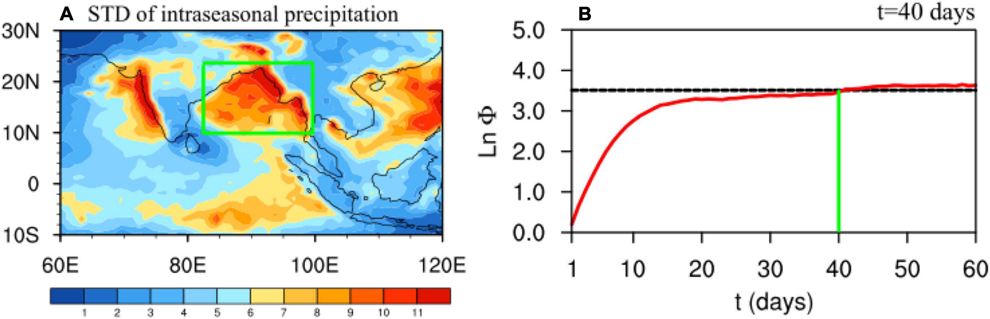
Figure 1. (A) The standard deviation of intraseasonal precipitation (mm/day) during boreal summer (June–September). (B) Mean error growth (red line) of the regional mean daily intraseasonal precipitation during boreal summer over 85–100°E and 10–24°N (green box in A) calculated by the NLLE method. The black dashed line marks the 98% level of the saturation value. The green line marks the predictability limit of 40 days.

TABLE 2

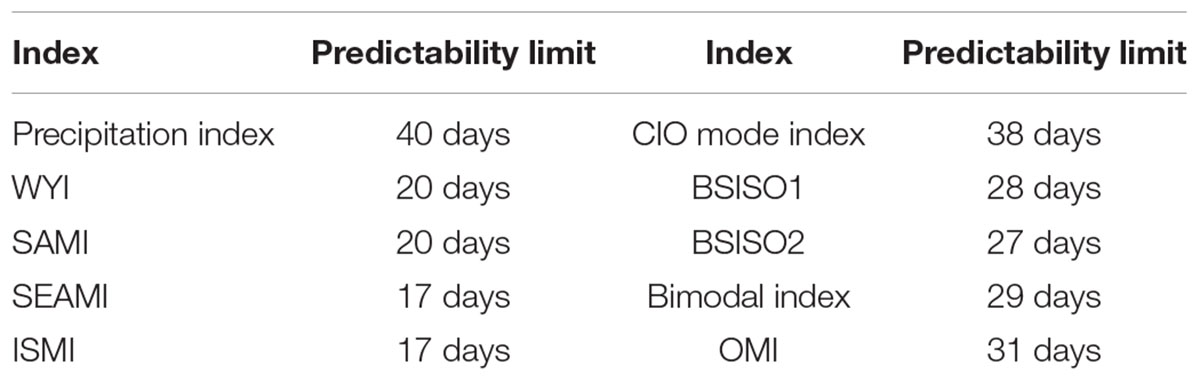
Table 2. The predictability limits of the indices (listed in Table 1) during boreal summer (June–September).

By analogy, the predictability limits (ln⁡Φ) of various dynamical monsoon and MISO indices (listed in Table 1) during boreal summer are examined with the NLLE method (Figure 2). When τ = 20 days, the mean error growth curves of the WYI (Figure 2A) and SAMI (Figure 2B) reach 98% of the saturation values (3.82 and 3.92, respectively). The predictability limits for the SEAMI (Figure 2C) and ISMI (Figure 2D) are about 17 days (listed in Table 2), and their 98% saturation levels are 3.70 and 3.67 (black dashed lines), respectively. All above monsoon indices have a predictability limit below 3 weeks, which is much lower than that of the precipitation index (∼40 days in Figure 1B). Hence, it is hard to fully materialize the predictability of monsoonal precipitation using the monsoon indices after four pentads. Using the NLLE method, the predictability limits of different BSISO indices (listed in Table 1) are also investigated (Figure 3). The 98% of the saturation values (black dashed lines in Figure 3) are 3.49, 3.38, 3.99, and 4.02 for BSISO1, BSISO2, the bimodal ISO index and OMI, respectively. The corresponding predictability limits are 28, 27, 29, and 31 days (listed in Table 2). Overall, the predictability limits of BSISO indices are around 30 days. Such a result is consistent with Ding et al. (2011), who applied the NLLE method and examined OLR, U850, and velocity potential at 200 hPa separately from May to September. Their results showed that the BSISO predictability limit was between 29 and 32 days. Comparing with the monsoon indices obtained with daily winds, all BSISO indices have longer predictability limits, although they are still shorter than the predictability limit of intraseasonal monsoonal precipitation (∼40 days in Figure 1B). Since the components are easier to forecast after removing the noises by filtering, one may envisage that the use of temporal filtering artificially prolongs the forecast skill. However, the influence of the filtered background noise is about 7 days (Seo et al., 2009; Ding et al., 2010), which is much lower than the predictability limit of intraseasonal oscillations. Thus, we can surmise that the estimated predictability of the intraseasonal variables is from the real signal of the physical process rather than the band-pass filtering.

FIGURE 2

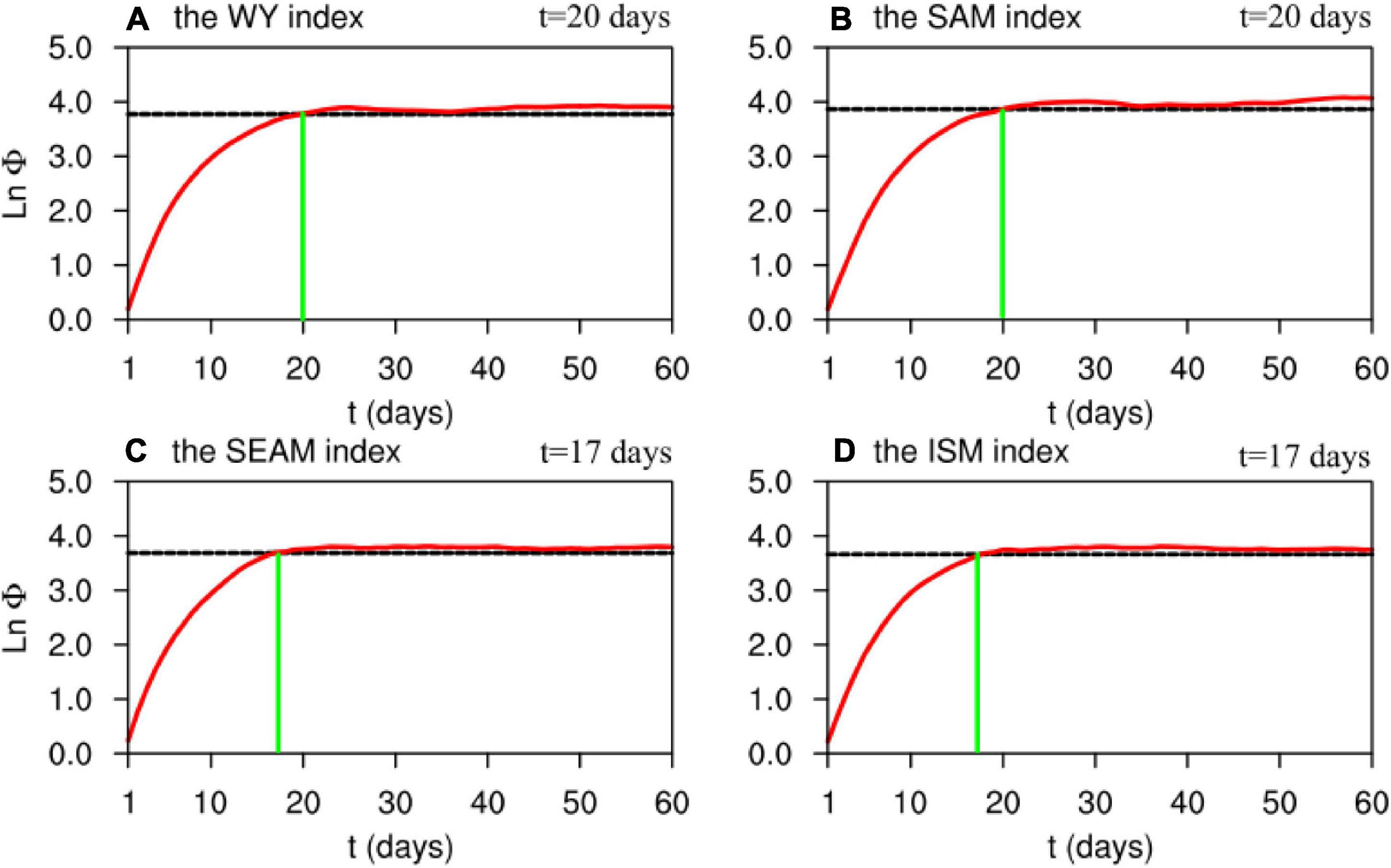
Figure 2. (A–D) Mean error growth (red line) of monsoon indices listed in Table 1. The black dashed line in each panel represents the 98% level of the saturation value. All results are based on the ERA5 reanalysis.

FIGURE 3

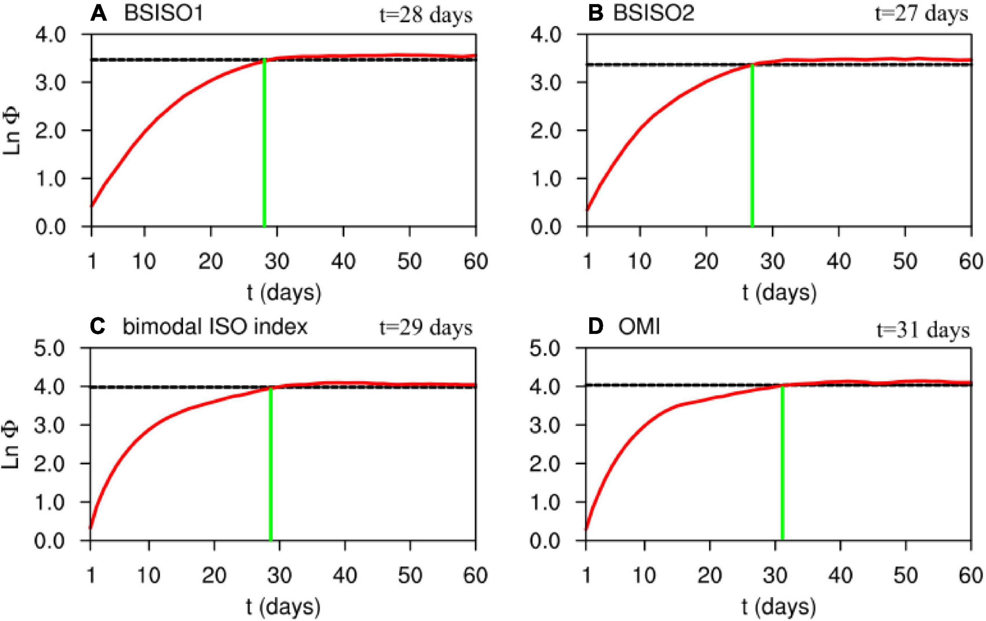
Figure 3. Same as Figure 2, but for (A) BSISO1 index, (B) BSISO2 index, (C) bimodal ISO index, and (D) OMI.

Previous studies have proven that the CIO mode is closely related to the ISM precipitation variability during boreal summer (Zhou et al., 2017a,2018). The CIO mode is obtained by the first C-EOF mode between intraseasonal SST anomalies and intraseasonal U850 anomalies. The CIO mode is robust and not sensitive to different reanalysis products, as shown with different data in Figures 4A,B. The positive phase of the CIO mode captures warm intraseasonal SST anomalies in the tropical Indian Ocean and an anti-cyclonic gyre in the lower troposphere over the Indian monsoon region. Such spatial structure is mainly attributable to less cloud due to an anticyclone, which allows more solar radiation onto the sea surface (Zhou et al., 2017a). The principal component of the first C-EOF mode is used as the CIO mode index (Figure 4C). The correlation coefficient of the two CIO mode indices is 0.98, which is significant at a 99% confidence level. Additionally, they have a high correlation with intraseasonal precipitation index during boreal summer (higher than 0.8). Figure 5 shows the correlation coefficients between the CIO mode index and the intraseasonal precipitation during boreal summer (from June to September). They are higher than 0.6 over the BoB (significant at the 99% confidence level), which implies a better prediction of ISM precipitation via the CIO mode index. The corresponding mean error growth curves (ln⁡Φ) of the CIO mode indices, which are obtained with different data, are shown in Figure 6. For the red line in Figures 6A,B, the saturation value is 3.62 (3.65). In both cases, the predictability limits of the CIO mode index are consistently around 38 days (listed in Table 2), which is closer to the predictability limit of monsoonal precipitation during ISM than other monsoon and BSISO indices.

FIGURE 4

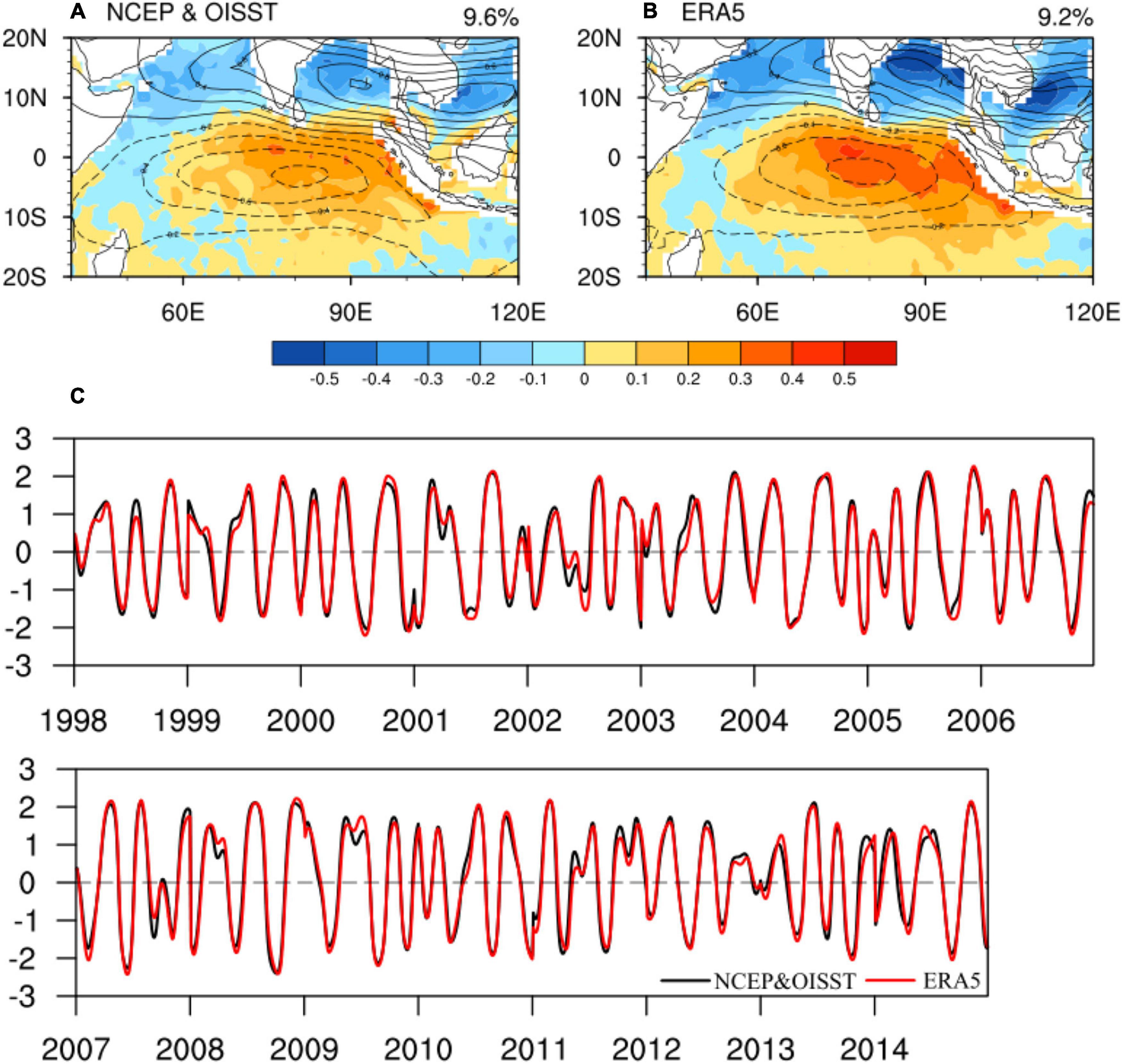
Figure 4. The positive phase of the CIO mode calculated with (A) NCEP and OISST and (B) ERA5 during the period of 1998–2014. The reddish is for the positive SST anomaly and the bluish is for the negative SST mode anomaly (°C). Solid contours are for positive zonal winds (westerly winds; m/s) and the dashed contours are for negative zonal winds (easterly winds). (C) The CIO mode indices associated with (A) (black line) and (B) (red line).

FIGURE 5

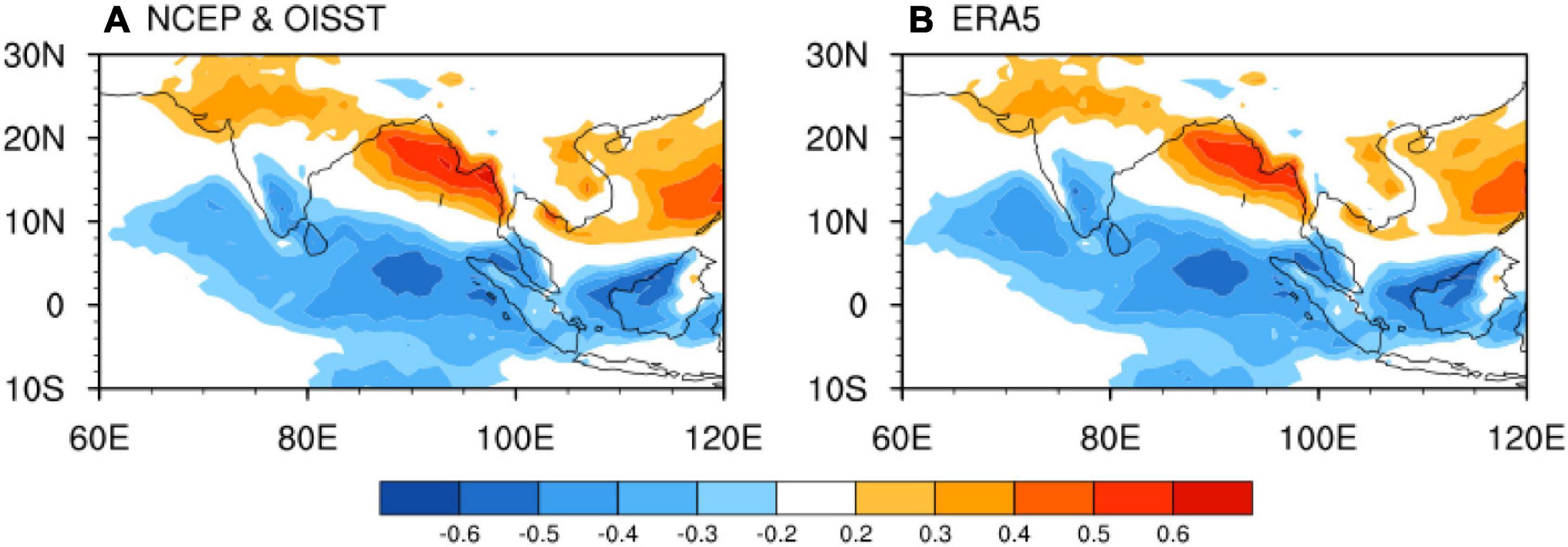
Figure 5. Correlation coefficients between intraseasonal precipitation anomalies and the CIO mode index obtained with (A) NCEP and OISST and (B) ERA5 during boreal summer (June–September).

FIGURE 6

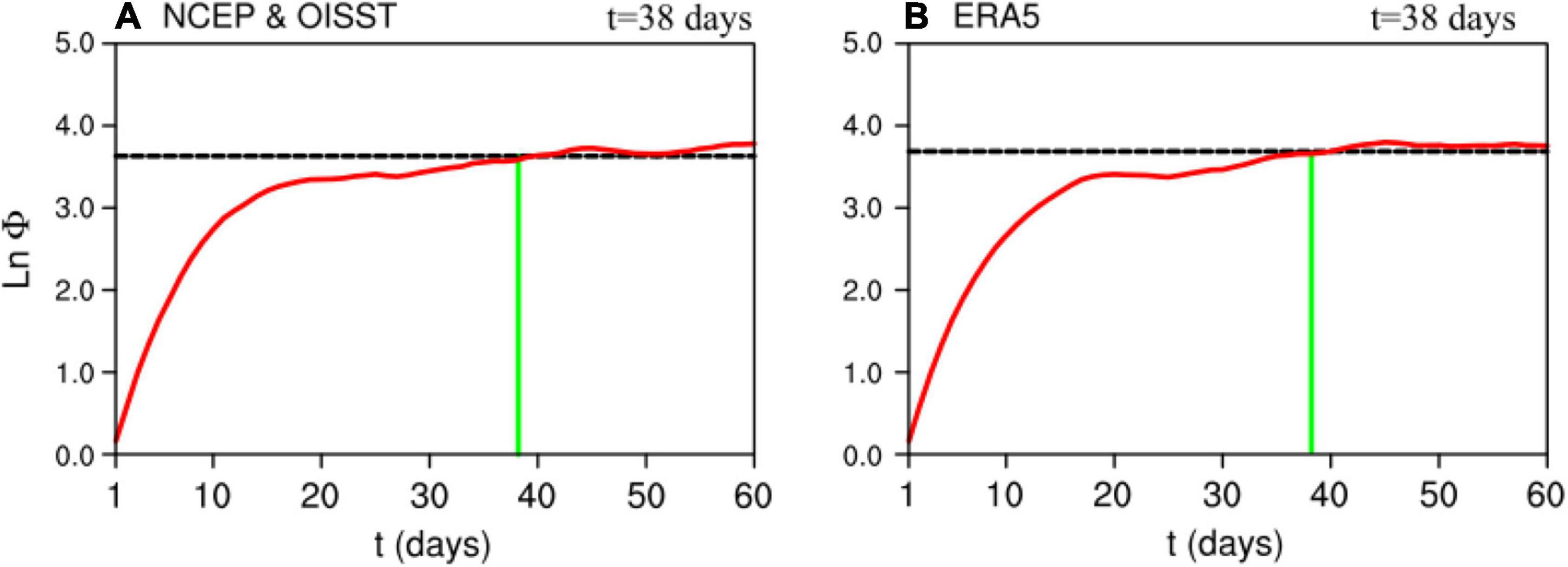
Figure 6. Mean error growth (red line) of the CIO mode index during boreal summer obtained with (A) NCEP and OISST and (B) ERA5. The black dashed line represents the 98% level of the saturation value.

To explore the reasons for the long predictability limit of the CIO mode index, the spatial distribution of the predictability limits of all key variables are calculated, including intraseasonal SST anomalies (Figure 7A), U850 anomalies (Figure 7B), and OLR anomalies (Figure 7C). For each grid point in Figures 7A–C, the NLLE method is applied to the time series at this grid point, and the predictability limit is determined following the same procedure as above. The right column in Figure 7 shows the ratio between the intraseasonal variance of each variable and its total variance. The specialty of the CIO mode, compared with all other indices, resides in the adoption of intraseasonal SST anomalies in technics. The predictability limit of intraseasonal SSTs is longer than 40 days over the tropical Indian Ocean (0–10°N, 60–95°E) and the western part of BoB (Figure 7A), where the intraseasonal SST anomalies are also large during the positive phase of CIO mode (contours in Figure 7D). The regions with long SST predictability limits also have significant intraseasonal SST variabilities, which is very likely to favor the high predictability of the CIO mode index. The other variable for the CIO mode is intraseasonal U850. The predictability limits of intraseasonal U850 are longer than 40 days from 15°N to the equator in the Northern Hemisphere and from 10°S to the equator in the Southern Hemisphere (Figure 7B), which are consistent with the two branches in the anticyclone of U850 in the CIO mode (contours in Figure 7E). Moreover, the intraseasonal U850 is also pronounced in these two regions (Figure 7E; Zhou et al., 2017b; Qin et al., 2020, 2021), so that large U850 variation contributes to high predictability of U850 which should be consequently favorable for high predictability of the CIO mode index. Furthermore, the CIO mode captures the coherent variabilities between the ocean and the atmosphere at the intraseasonal timescales. Figure 8A shows the first EOF mode of intraseasonal SST anomalies alone (without a combination with intraseasonal U850 anomalies). The spatial pattern is a west-east dipole structure, and its time series do not have a significant relation with monsoonal precipitation (Figure 8B). However, it is not the IOD, since the EOF is conducted with the intraseasonal variabilities. The central tropical Indian Ocean is the node of the SST-alone mode, where the variation is small. The different spatial patterns between the CIO mode and the SST-alone mode are attributable to the ocean-atmosphere interactions, since the former seeks the maximum co-variance between the intraseasonal SST anomalies and intraseasonal U850 anomalies. Therefore, the match between the long predictability limit of SST in the central tropical Indian Ocean (Figure 7A) and the CIO mode (Figure 7D) sheds light on the importance of the ocean-atmosphere interaction, which is well captured by the CIO mode, for improving the intraseasonal monsoonal rainfall. Moreover, it is pointed out by Ding et al. (2010) that the initial conditions may play an important role in determining the rapid initial error growth, but subsequently the error growth may be more strongly influenced by the slowly varying boundary conditions, such as the SSTs. In contrast, other MISO indices adopt OLR alone (such as Bimodal ISO index and OMI) or a combination between U850 and OLR (such as BSISO1 and BSISO2). The OLR has maximum predictability limits along the Somali coast and the western tropical Indian Ocean. However, these regions are not the key regions for convection during the ISM. Therefore, pronounced OLR anomalies in the monsoon region, particularly over the BoB, contribute little to prolong the predictability of the MISO indices which are built on the OLR alone. BSISO1 and BSISO2 are likely to be subject to the low predictability of OLR anomalies in the monsoon region (particularly over the BoB), since OLR is one component in these two indices. Moreover, as shown in Figures 2, 3 in Lee et al. (2013), the OLR anomalies in the first four EOF modes are weak along the Somali coast, so that the high predictability of OLR in that region cannot be utilized. In addition, for BSISO1, the U850 anomalies of the second EOF mode are small from 10°S to the equator (Figure 2 in Lee et al., 2013). As a result, BSISO1 cannot take advantage of the long predictability of U850 in the Southern Hemisphere (Figure 7B). Similarly, for BSISO2, the U850 anomalies from 10°S to the equator are small (Figure 3 in Lee et al., 2013), and the high predictability of U850 cannot be fully taken advantage of, either.

FIGURE 7

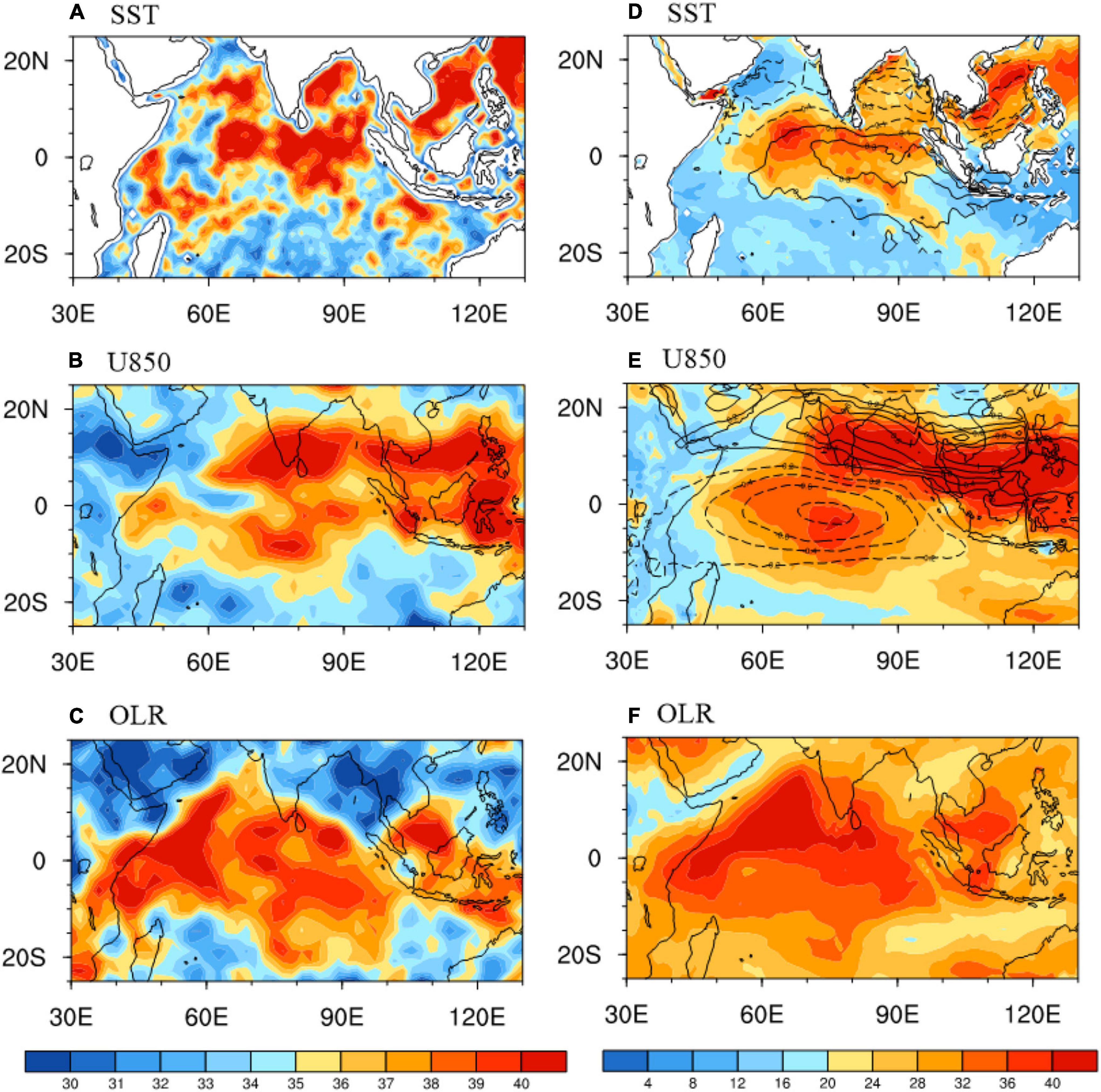
Figure 7. (A) Spatial distribution of the predictability limits of intraseasonal SST during boreal summer from 1998 to 2014. (B,C) Are the same as (A), but for intraseasonal U850 and intraseasonal OLR. (D) Ratio between the intraseasonal variance and the total variance of SST during boreal summer from 1998 to 2014. The superimposed contours are the SST mode of the positive CIO mode (same as the color shades in Figure 4B). (E,F) Are the same as (D), but for U850 and OLR. The contours in (E) are the U850 mode of the positive CIO mode (same as the contours in Figure 4B). All the results are based on the ERA5 reanalysis.

FIGURE 8

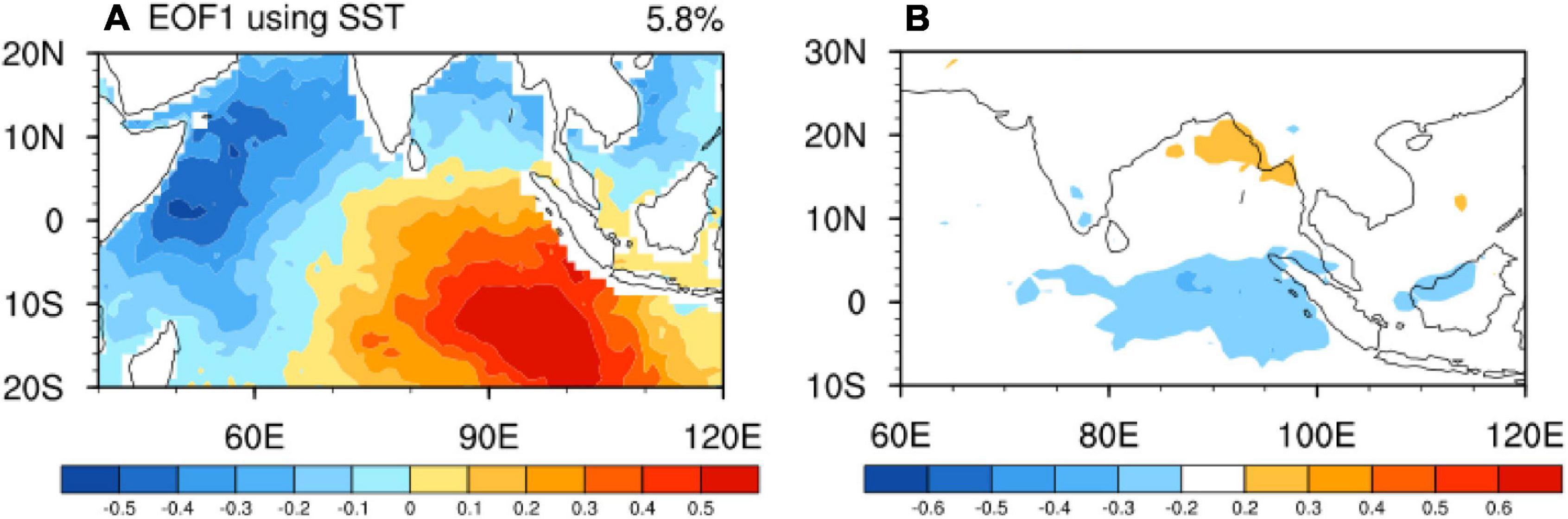
Figure 8. (A) The spatial structure of the first EOF mode using SST (°C) calculated with ERA5 reanalysis during the period of 1998–2014. (B) Correlation coefficients between intraseasonal precipitation anomalies and the PC1 during boreal summer (June–September).

Summary and Discussion

Given the close relationship between the CIO mode and the ISM precipitation variability, the predictability limit of the CIO mode index is examined using the NLLE method, which provides a quantitative estimate on the atmospheric and oceanic predictability. It shows that the predictability limit of the CIO mode index can reach 38 days during boreal summer (June–September), which is not sensitive to different reanalysis products. The predictability limit of the CIO mode index is higher than that of well-known monsoon indices and BSISO indices based on the NLLE method. It is also found that the intraseasonal SST and U850 have a large variance in the ISM region with the predictability limits over 40 and 45 days, respectively, which are higher than that of intraseasonal OLR. As a result, the CIO mode index shows a longer predictability limit, which is expected to improve the practical prediction skill of monsoon precipitation during the ISM.

Based on the improvements in the simulation of climate models, the prediction skill of monsoons has significantly improved in recent decades (Liu et al., 2013). However, it is confirmed by model studies, such as in the NCEP Climate Forecast System version 2 (CFSv2, Liu et al., 2013) and the S2S database (Jie et al., 2017), that the high skills of monsoon indices are only about 2 weeks. Some studies discovered the important effects of air-sea interactions in improving the prediction skill of monsoon in models (e.g., Yoo et al., 2006; Fu et al., 2007, 2008; Goswami et al., 2014; Chowdary et al., 2016). As shown with the CIO mode, a better reproduction of coordinated variation between the atmosphere and the ocean can help to extend monsoonal precipitation forecast and predict the ISM more accurately.

Although the number of studies on intraseasonal to seasonal variabilities including the prediction of the monsoon onset and retreat has increased in recent years (e.g., Fu et al., 2007; Liu et al., 2013; Zhou and Murtugudde, 2014; Jie et al., 2017; Zhou et al., 2019), the prediction of the amplitude and frequency of monsoon rainfall remains difficult. Since the CIO mode index has a high linear correlation with the monsoon precipitation, it provides a new avenue to capture the amplitude and frequency of the ISM. Besides, it is worth to discover the linkage between the CIO mode and the onset/withdraw dates of ISM. Moreover, previous studies also revealed that the CIO mode represents the mechanistic link between the thermodynamic and dynamic fields during the ISM not only in observations but also in current models (Zhou et al., 2017a,2018; Li et al., 2020; Qin et al., 2020, 2021). However, unfortunately, the simulation of the CIO mode is still a challenge in state-of-the-art models. The biases in the CIO mode simulation are mainly attributable to the weak meridional gradient of low-level background zonal winds, which reduces the barotropic kinetic energy conversion from the background state to intraseasonal variabilities. In addition, the force and response relation between the atmosphere and the ocean associated with the CIO mode is even opposite in CESM (Zhou et al., 2018). Further improvements in convection parameterization schemes by numerical experiments may help us to better understand the important roles of the air-sea interactions and barotropic instability for the CIO mode generation, which will in turn be helpful for the betterment of MISO and the ISM precipitation forecast.

Data Availability Statement

The original contributions presented in the study are included in the article/Supplementary Material, further inquiries can be directed to the corresponding author/s.

Author Contributions

JQ, LZ, RD, and BL contributed to conception and design of the study. All authors contributed to the article and approved the submitted version.

Funding

This work was supported by grants from the National Natural Science Foundation of China (Nos. 42106003, 42076001, and 42125601), the Fundamental Research Funds for the Central Universities (No. B210202142), Innovation Group Project of Southern Marine Science and Engineering Guangdong Laboratory (Zhuhai) (No. 311020004), and the Oceanic Interdisciplinary Program of Shanghai Jiao Tong University (No. SL2020PT205).

Conflict of Interest

The authors declare that the research was conducted in the absence of any commercial or financial relationships that could be construed as a potential conflict of interest.

Publisher’s Note

All claims expressed in this article are solely those of the authors and do not necessarily represent those of their affiliated organizations, or those of the publisher, the editors and the reviewers. Any product that may be evaluated in this article, or claim that may be made by its manufacturer, is not guaranteed or endorsed by the publisher.

Acknowledgments

We thank Jianping Li and RD for developing the NLLE method. All observation data and reanalysis products for this manuscript are properly cited and referred to in the reference list.

Supplementary Material

The Supplementary Material for this article can be found online at: https://www.frontiersin.org/articles/10.3389/fmars.2021.809798/full#supplementary-material

References

Abhilash, S., Sahai, A., Borah, N., Chattopadhyay, R., Joseph, S., Sharmila, S., et al. (2014). Prediction and monitoring of monsoon intraseasonal oscillations over Indian monsoon region in an ensemble prediction system using CFSv2. Clim. Dyn. 42, 2801–2815. doi: 10.1007/s00382-013-2045-9

CrossRef Full Text | Google Scholar

Chattopadhyay, R., Sahai, A., and Goswami, B. (2008). Objective identification of nonlinear convectively coupled phases of monsoon intraseasonal oscillation: implications for prediction. J. Atmos. Sci. 65, 1549–1569. doi: 10.1175/2007JAS2474.1

CrossRef Full Text | Google Scholar

Chowdary, J., Parekh, A., Ojha, S., Gnanaseelan, C., and Kakatkar, R. (2016). Impact of upper ocean processes and air–sea fluxes on seasonal SST biases over the tropical Indian Ocean in the NCEP Climate Forecasting System. Int. J. Climatol. 36, 188–207. doi: 10.1002/joc.4336

CrossRef Full Text | Google Scholar

Ding, R., and Li, J. (2007). Nonlinear finite-time Lyapunov exponent and predictability. Phys. Lett. A 364, 396–400. doi: 10.1016/j.physleta.2006.11.094

CrossRef Full Text | Google Scholar

Ding, R., Li, J., and Ha, K. (2008). Trends and interdecadal changes of weather predictability during 1950s–1990s. J. Geophys. Res. 113:D24112. doi: 10.1029/2008JD010404

CrossRef Full Text | Google Scholar

Ding, R., Li, J., and Seo, K. (2010). Predictability of the Madden-Julian oscillation estimated using observational data. Mon. Weather Rev. 138, 1004–1013. doi: 10.1175/2009MWR3082.1

CrossRef Full Text | Google Scholar

Ding, R., Li, J., and Seo, K. (2011). Estimate of the predictability of boreal summer and winter intraseasonal oscillations from observations. Mon. Weather Rev. 139, 2421–2438. doi: 10.1175/2011MWR3571.1

CrossRef Full Text | Google Scholar

Fu, X., Lee, J., Wang, B., Wang, W., and Vitart, F. (2013). Intraseasonal forecasting of the Asian summer monsoon in four operational and research models. J. Clim. 26, 4186–4203. doi: 10.1175/JCLI-D-12-00252.1

CrossRef Full Text | Google Scholar

Fu, X., Wang, B., Waliser, D., and Tao, L. (2007). Impact of atmosphere-ocean coupling on the predictability of monsoon intraseasonal oscillations. J. Atmos. Sci. 64, 157–174. doi: 10.1175/JAS3830.1

CrossRef Full Text | Google Scholar

Fu, X., Yang, B., Bao, Q., and Wang, B. (2008). Sea surface temperature feedback extends the predictability of tropical intraseasonal oscillation. Mon. Weather Rev. 136, 577–597. doi: 10.1175/2007MWR2172.1

CrossRef Full Text | Google Scholar

Goswami, B. N. (2005). “South Asian monsoon,” in Intraseasonal Variability in the Atmosphere-Ocean Climate System, eds W. K. M. Lau and D. E. Waliser (Berlin: Springer), 19–61. doi: 10.1007/3-540-27250-X_2

CrossRef Full Text | Google Scholar

Goswami, B., and Xavier, P. (2003). Potential predictability and extended range prediction of Indian summer monsoon breaks. Geophys. Res. Lett. 30:1966. doi: 10.1029/2003GL017810

CrossRef Full Text | Google Scholar

Goswami, B., Deshpande, M., Mukhopadhyay, P., Saha, S., Rao, S. A., and Murthugudde, R. (2014). Simulation of monsoon intraseasonal variability in NCEP CFSv2 and its role on systematic bias. Clim. Dyn. 43, 2725–2745. doi: 10.1007/s00382-014-2089-5

CrossRef Full Text | Google Scholar

Goswami, B., Krishnamurthy, V., and Annmalai, H. (1999). A broad-scale circulation index for the interannual variability of the Indian summer monsoon. Q. J. R. Meteorol. Soc. 125, 611–633. doi: 10.1002/qj.49712555412

CrossRef Full Text | Google Scholar

Hersbach, H., Bell, B., Berrisford, P., Horányi, A., Sabater, J. M., Nicolas, J., et al. (2019). Global reanalysis: goodbye ERA-Interim, hello ERA5. ECMWF Newsl. 159, 17–24. doi: 10.21957/vf291hehd7

CrossRef Full Text | Google Scholar

Huffman, G., Bolvin, D., Nelkin, E., Wolff, D., Adler, R., Gu, G., et al. (2007). The TRMM multisatellite precipitation analysis (TMPA): quasi-global, multiyear, combined-sensor precipitation estimates at fine scales. J. Hydrometeorol. 8, 38–55. doi: 10.1175/JHM560.1

CrossRef Full Text | Google Scholar

Jie, W., Vitart, F., Wu, T., and Liu, X. (2017). Simulations of the Asian summer monsoon in the sub-seasonal to seasonal prediction project (S2S) database. Q. J. R. Meteorol. Soc. 143, 2282–2295. doi: 10.1002/qj.3085

CrossRef Full Text | Google Scholar

Kalnay, E., Kanamitsu, M., Kistler, R., Collins, W., Deaven, D., Gandin, L., et al. (1996). The NCEP/NCAR 40-year reanalysis project. Bull. Am. Meteorol. Soc. 77, 437–472.

Google Scholar

Kikuchi, K., Wang, B., and Kajikawa, Y. (2012). Bimodal representation of the tropical intraseasonal oscillation. Clim. Dyn. 38, 1989–2000. doi: 10.1007/s00382-011-1159-1

CrossRef Full Text | Google Scholar

Kiladis, G., Dias, J., Straub, K. H., Wheeler, M., Tulich, S. N., Kikuchi, K., et al. (2014). A comparison of OLR and circulation-based indices for tracking the MJO. Mon. Weather Rev. 142, 1697–1715. doi: 10.1175/MWR-D-13-00301.1

CrossRef Full Text | Google Scholar

Lee, J., Wang, B., Wheeler, M., Fu, X., Waliser, D., and Kang, I. (2013). Real-time multivariate indices for the boreal summer intraseasonal oscillation over the Asian summer monsoon region. Clim. Dyn. 40, 493–509. doi: 10.1007/s00382-012-1544-4

CrossRef Full Text | Google Scholar

Li, B., Ding, R., Li, J., Xu, Y., and Li, J. (2018). Asymmetric response of predictability of East Asian summer monsoon to ENSO. SOLA 14, 52–56. doi: 10.2151/sola.2018-009

PubMed Abstract | CrossRef Full Text | Google Scholar

Li, B., Zhou, L., Wang, C., Gao, C., Qin, J., and Meng, Z. (2020). Modulation of tropical cyclone genesis in the Bay of Bengal by the Central Indian Ocean mode. J. Geophys. Res. 125:e2020JD032641. doi: 10.1029/2020JD032641

CrossRef Full Text | Google Scholar

Li, J., and Ding, R. (2011). Temporal-Spatial distribution of atmospheric predictability limit by local dynamical analogs. Mon. Weather Rev. 139, 3265–3283. doi: 10.1175/MWR-D-10-05020.1

CrossRef Full Text | Google Scholar

Liu, X., Yang, S., Li, Q., Kumar, A. S., Weaver, S., and Liu, S. (2013). Subseasonal forecast skills and biases of global summer monsoons in the NCEP Climate Forecast System version 2. Clim. Dyn. 42, 1487–1508. doi: 10.1007/s00382-013-1831-8

CrossRef Full Text | Google Scholar

Meng, Z., Zhou, L., Murtugudde, R., Yang, Q., Pujiana, K., and Xi, J. (2021). Tropical oceanic intraseasonal variabilities associated with central Indian Ocean mode. Clim. Dyn. 1–20. doi: 10.1007/s00382-021-05951-1

CrossRef Full Text | Google Scholar

Qin, J., Zhou, L., Li, B., and Murtugudde, R. (2020). Simulation of Central Indian Ocean Mode in S2S models. J. Geophys. Res. Atmos. 125:e2020JD033550. doi: 10.1029/2020JD033550

CrossRef Full Text | Google Scholar

Qin, J., Zhou, L., Meng, Z., Li, B., Lian, T., and Murtugudde, R. (2021). Barotropic energy conversion during Indian summer monsoon: implication of central Indian Ocean mode simulation in CMIP6. Clim. Dyn. doi: 10.21203/rs.3.rs-715759/v1

CrossRef Full Text | Google Scholar

Reynolds, R. W., Smith, T. M., Liu, C., Chelton, D. B., Casey, K. S., and Schlax, M. G. (2007). Daily high-resolution-blended analyses for sea surface temperature. J. Clim. 20, 5473–5496. doi: 10.1175/2007JCLI1824.1

CrossRef Full Text | Google Scholar

Rogberg, P., Read, P., Lewis, S., and Montabone, L. (2010). Assessing atmospheric predictability on Mars using numerical weather prediction and data assimilation. Q. J. R. Meteorol. Soc. 136, 1614–1635. doi: 10.1002/qj.677

CrossRef Full Text | Google Scholar

Sabeerali, C. T., Ramu Dandi, A., Dhakate, A., Salunke, K., Mahapatra, S., and Rao, S. A. (2013). Simulation of boreal summer intraseasonal oscillations in the latest CMIP5 coupled GCMs. J. Geophys. Res. Atmos. 118, 4401–4420. doi: 10.1002/jgrd.50403

CrossRef Full Text | Google Scholar

Sahai, A. K., and Chattopadhyay, R. (2006). An Objective Study of Indian Summer Monsoon Variability Using the Self Organizing Map Algorithms. IITM Research Report, No.113. Pune: Indian Institute of Tropical Meteorology.

Google Scholar

Seo, K., Wang, W., Gottschalck, J., Zhang, Q., Schemm, J., Higgins, W., et al. (2009). Evaluation of MJO forecast skill from several statistical and dynamical forecast models. J. Clim. 22, 2372–2388. doi: 10.1175/2008JCLI2421.1

CrossRef Full Text | Google Scholar

Shukla, R. P. (2014). The dominant intraseasonal mode of intraseasonal South Asian summer monsoon. J. Geophys. Res. Atmos. 119, 635–651. doi: 10.1002/2013JD020335

CrossRef Full Text | Google Scholar

Waliser, D. E. (2006). “Intraseasonal variability,” in The Asian Monsoon, ed. B. Wang (Berlin: Springer), 203–257.

Google Scholar

Wang, B., and Fan, Z. (1999). Choice of South Asian summer monsoon indices. Bull. Am. Meteorol. Soc. 80, 629–638.

Google Scholar

Wang, B., Kang, I. S., and Lee, J. Y. (2004). Ensemble simulations of Asian–Australian monsoon variability by 11 AGCMs. J. Clim. 17, 803–818.

Google Scholar

Wang, B., Wu, R., and Lau, K. (2001). Interannual variability of the asian summer monsoon: contrasts between the Indian and the western north pacific–east Asian monsoons*. J. Clim. 14, 4073–4090.

Google Scholar

Webster, P., and Yang, S. (1992). Monsoon and Enso: selectively interactive systems. Q. J. R. Meteorol. Soc. 118, 877–926. doi: 10.1002/qj.49711850705

CrossRef Full Text | Google Scholar

Yoo, S., Yang, S., and Ho, C. (2006). Variability of the Indian Ocean sea surface temperature and its impacts on Asian-Australian monsoon climate. J. Geophys. Res. 111:D03108. doi: 10.1029/2005JD006001

CrossRef Full Text | Google Scholar

Zhou, L., and Murtugudde, R. (2014). Impact of northward-propagating intraseasonal variability on the onset of Indian summer monsoon. J. Clim. 27, 126–139. doi: 10.1175/JCLI-D-13-00214.1

CrossRef Full Text | Google Scholar

Zhou, L., Murtugudde, R., Chen, D., and Tang, Y. (2017a). A Central Indian Ocean mode and heavy precipitation during the Indian summer monsoon. J. Clim. 30, 2055–2067. doi: 10.1175/JCLI-D-16-0347.1

CrossRef Full Text | Google Scholar

Zhou, L., Murtugudde, R., Chen, D., and Tang, Y. (2017b). Seasonal and interannual variabilities of the central Indian Ocean mode. J. Clim. 30, 6505–6520. doi: 10.1175/JCLI-D-16-0616.1

CrossRef Full Text | Google Scholar

Zhou, L., Murtugudde, R., Neale, R. B., and Jochum, M. (2018). Simulation of the Central Indian Ocean mode in CESM: implications for the Indian summer monsoon system. J. Geophys. Res. Atmos. 123, 58–72. doi: 10.1002/2017JD027171

CrossRef Full Text | Google Scholar

Zhou, Z. Q., Zhang, R., and Xie, S. P. (2019). Interannual variability of summer surface air temperature over central India: implications for monsoon onset. J. Clim. 32, 1693–1706. doi: 10.1175/JCLI-D-18-0675.1

CrossRef Full Text | Google Scholar