Alongshore Propagation of Subtidal Sea Level Fluctuations Around the Korean Peninsula Over Varying Stratification and Shelf Topography

Introduction

Understanding subtidal (defined as a period from 3 to 20 days) coastal sea level variability is important for effectively adapting to rising global and regional sea levels (Stammer et al., 2013). Subtidal coastal sea level variability is often explained by alongshore propagating coastal-trapped waves (CTWs), which play an important role in coastal ocean circulation and turbulent mixing on continental slopes (Hughes et al., 2019; Schlosser et al., 2019). The CTWs generated by alongshore wind forcing propagate thousands of kilometers away along the coast with changing phase speeds due to local density stratification and shelf bottom topography (Wang and Mooers, 1976; Huthnance, 1978; Brink, 1982; Battisti and Hickey, 1984; Hughes et al., 2019; Schlosser et al., 2019). The subtidal sea level fluctuations in many coastal areas related to stratification and shelf topography have been studied using a classical CTW model; for example, phase speeds ranging from 2.72 to 14.10 m s^–1 off the South African coast varying with shelf widths of 10–100 km (Schumann and Brink, 1990) and phase speeds ranging from 1.83 to 4.43 m s^–1 off the west coast of India varying with shelf widths of 50–80 km (Amol et al., 2012).

However, owing to the assumptions of classical CTW theory, namely a straight coastline or limited consideration for external forcing (e.g., only alongshore wind forcing is considered), the CTW model often results in sea level fluctuations that are significantly different from the observations (Cho et al., 2014; Brunner et al., 2019). Recent studies have pointed out that the classic CTW model is not universally applicable to most coastlines that do not meet the required assumptions of a straight coastline with similar shelf topography (Brunner et al., 2019). The coastal areas around the Korean Peninsula (KP) are one such region where the assumptions for the CTW model cannot be optimally satisfied (Figure 1). The regions off the coasts around the KP consist of contrasting shelf topographies between the west and south coasts with a shallow and gentle (<0.003) slope connected to the Yellow and East China Sea and the east coast with a deep and steep (>0.01) slope connected to the East Sea (Japan Sea). Despite some previous studies explaining the subtidal coastal sea level fluctuations around the KP based on the classical CTW model under varying conditions of stratification and shelf topography (Lee and Chung, 1982; Lyu et al., 2002; Cho et al., 2014), the reasons for the significant difference between the observed (6.1–15.6 m s^–1) and modeled (4.6–10.3 m s^–1) propagation speeds are still poorly understood (Cho et al., 2014). In contrast, the subtidal sea level fluctuations off the east coast of the KP are also related to non-isostatic sea level responses to atmospheric pressure disturbances over a period of 2–20 days (Lyu et al., 2002; Nam et al., 2004; Jung et al., 2008), as well as a local upwelling/downwelling response to alongshore wind forcing beyond CTW dynamics (Park and Nam, 2018). Thus, our understanding of subtidal sea level fluctuations around the KP is far from complete; for example, how well the subtidal sea level fluctuations can be explained using the classic CTW and other dynamics beyond CTWs are poorly understood.

FIGURE 1

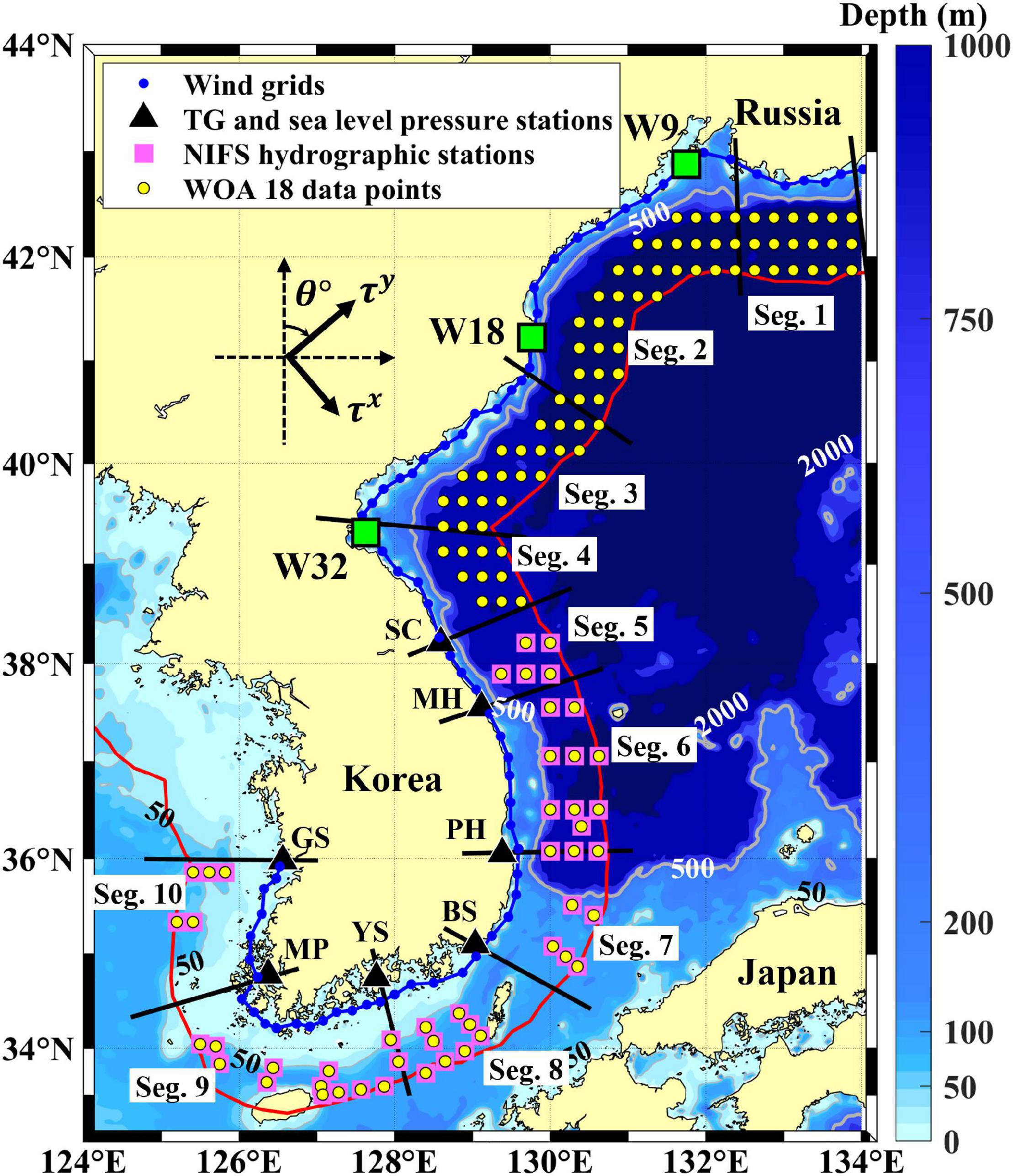
Figure 1. Bottom topography around the Korean Peninsula (KP). Water depth is shown with colors and contours, where 50 and 500 m isobaths are highlighted by thin and thick lines, respectively. Coastal zones (between coastline denoted with blue line and offshore boundary 100 km distant from the coastline denoted with red line) off the north coast (Segs. 1–4), east coast (Segs. 5–7), south coast (Segs. 8–9), and west coast (Seg. 10) of the KP are divided into 10 segments (Segs. 1–10; labeled) as marked by thick black lines. The grid points for wind stress data (wind grids) are denoted by blue circles along the coast. Locations of the tide-gauge (TG) sea level stations along the coasts around the KP, three wind grids (W9, W18, and W32), stations for the South Korea National Institute of Fisheries Science (NIFS) hydrographic observation, and World Ocean Atlas 2018 (WOA18) data grids are denoted with black triangles, green squares, pink squares, and yellow circles, respectively. The coordinate system for sea surface wind stresses (τ^x, τ^y) and currents, with a rotation angle, θ, measured clockwise from the north, are marked with thick arrows.

This study aims to (1) Characterize alongshore propagations of subtidal sea level fluctuations observed around the KP, (2) Address the characteristics of modeled leading mode wind-forced CTWs propagating along the coasts under seasonally varying stratification, and (3) Discuss common and consistent features and differences between observed and modeled alongshore propagations. The observational data and CTW model applied in this study are described in section “Data and Methods.” Both the observational and modeling results are presented in section “Results” and discussed in section “Discussion,” the conclusions are presented in section “Conclusion.”

Data and Methods

Data Sources

Sea levels recorded every minute and averaged with an interval of 1 h at seven coastal tide-gauge (TG) stations around the KP – Sokcho (SC), Mukho (MH), Pohang (PH), Busan (BS), Yeosu (YS), Mokpo (MP), and Gunsan (GS) – were used in this study (Figure 1). The TG sea level data spans 21 years, from January 1997 to December 2017. Sea level fluctuations on the west and south coasts (BS, YS, MP, and GS) are generally much larger due to a higher tidal range of up to several meters, as compared with that along the east coast (SC, MH, and PH). Hourly sea level atmospheric pressures observed near the TG stations were used to correct the TG sea levels for the effect of atmospheric pressure loading required to extract sea level fluctuations dynamically linked to subsurface pressure perturbation.

Sea surface wind stress data from Copernicus Marine Environment Monitoring Service (CMEMS) blended satellite-observed wind products with a time interval of 6 h and a spatial resolution of 0.25° × 0.25° were used to simulate the wind-driven subtidal coastal sea level fluctuations. Such blended wind products have been widely used, but low performances for coastal areas compared to offshore areas have been reported (Bentamy, 2019). Moreover, satellite-observed wind products may have an issue with quality, often yielding significant differences from in situ measured winds, as also reported for the study region, e.g., near the east coast of the KP due to the orographic effect (Nam et al., 2005). Although recent satellite wind products such as the CMEMS blended wind provide reasonable patterns of spatio-temporal wind variations (Bentamy et al., 2021), the data were compared with the wind products of Modern-Era Retrospective analysis for Research and Applications version 2 (MERRA2) with a time interval of 6 h and a spatial resolution of 0.50° × 0.33° (Gelaro et al., 2017). The CMEMS and MERRA2 wind stress data at 74 grid points (W1–W74) from January 1997 to December 2017 were selected to use considering the typical wavelength of mode-1 CTWs (100–1,000 km) and the locations of the seven TG stations (Figure 1 and Supplementary Table 1).

Bottom topography data gridded with 2-arc minute grids within 100 km of the coastline were used to characterize the shelf topography. To characterize the seasonal density stratifications around the KP, vertical profiles of the water temperature (T) and practical salinity (S) were obtained from ship-based hydrographic data provided by the South Korea National Institute of Fisheries Science (NIFS). The NIFS hydrographic data collected at 15 standard depths (0, 10, 20, 30, 50, 75, 100, 125, 150, 200, 250, 300, 350, 400, and 500 m; red horizontal grid lines in Figure 2k) have been provided on a bi-monthly basis at nominal stations around the KP since 1961; the data collected at selected stations around the KP (offshore region 50–100 km distant from the coast; pink squares in Figure 1) from 1997 to 2017 were used here. To supplement the hydrographic data, particularly for the northern part of the east coast of the KP where NIFS data are not available (Figure 1), World Ocean Atlas 2018 (WOA18) data were used, which are monthly averaged annual vertical climatology (12 datasets) profiles of temperature and salinity, constructed with a spatial resolution of 0.25° × 0.25°. The 82 grids from the WOA18 data around the northern part of the east coast of the KP and an additional 48 grids from the WOA18 data matching the NIFS stations were selected (Figure 1).

FIGURE 2

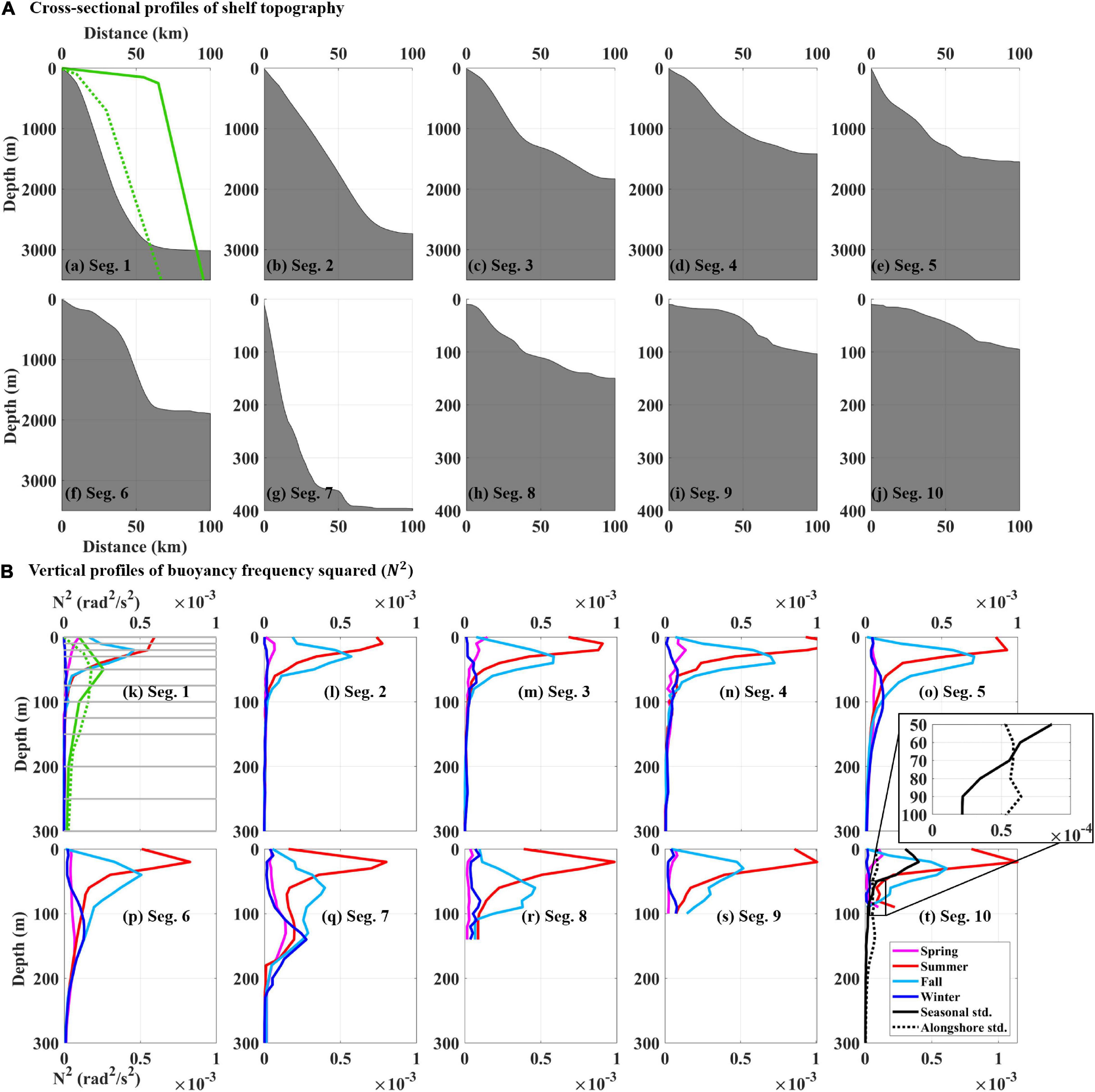
Figure 2. (A) Cross-sectional profiles of the shelf topography within the coastal area around the KP [Segs. 1–10; from (a–j)] and (B) vertical profiles of the squared buoyancy frequency (N²) averaged over four seasons (spring, summer, fall, and winter; pink, red, sky blue, and blue colors, respectively) for 10 segments [Segs. 1–10; from (k–t)] at the upper 300 m. In (a–j), water depth (y-axis) ranges from the surface to 3,500 m for Segs. 1–6 and 400 m for Segs. 7–10, respectively. In (a,k), the cross-sectional profiles of shelf topography and vertical profiles of N² for the East Australian coast (Church et al., 1986) and west coast of Peru (Brink, 1982; Illig et al., 2018) are overlaid with green solid and dotted lines, respectively. In (k), the 15 standard depths of the NIFS hydrographic observations are denoted by gray horizontal lines. In (t), standard deviations from the seasonal-mean and alongshore-mean N² (seasonal std. and alongshore std.) are shown with black solid and dashed lines, respectively, and zoomed in at depths 50–100 m.

Data Processing

The coastline was defined as a location where the water depth is ≤10 m, matching grids for wind stress data (wind grids) in an alongshore interval of 14–40 km. Local coastline directions were determined as the direction connecting two neighboring coastline locations. A local coordinate system was used to determine the alongshore (y) and cross-shore (x) directions, where the alongshore direction was defined as a direction rotated clockwise from due north by θ, which is the same as the local coastline direction by definition (Supplementary Table 1 and Figure 1). The sea surface wind stress was decomposed into alongshore (τ^y) and cross-shore (τ^x) components as ${\mathrm{\tau }}^y={\mathrm{\tau }}_0^{x}sin(\mathrm{\theta })+{\mathrm{\tau }}_0^{y}cos(\mathrm{\theta })$ and ${\mathrm{\tau }}^x={\mathrm{\tau }}_0^{x}cos(\mathrm{\theta })-{\mathrm{\tau }}_0^{y}sin(\mathrm{\theta })$ with positive up-shelf (e.g., poleward on the east coast, eastward on the south coast, and equatorward on the west coast) and positive seaward, respectively, where ${\mathrm{\tau }}_0^x$ and ${\mathrm{\tau }}_0^y$ denote the eastward and northward wind stresses, respectively. The term “remote,” as opposed to “local,” location was defined here as a location more distant than one wind stress or coastline grid away from the reference location. To the north of the northernmost TG station (SC) along the east coast, three grids for wind stress (W9, W18, and W32; squares in Figure 1), which well-represent regional wind patterns, were selected for comparisons of regional wind and observed TG sea levels (η_obs). The 6-hourly alongshore and cross-shore wind stresses (τ^y and τ^x) from both CMEMS and MERRA2 wind products were linearly interpolated to yield hourly time-series matching η_obs. The ocean tides were removed from η_adj using the tidal level prediction program known as the Unified Tidal Analysis and Prediction (UTide) developed for the MATLAB software (Codiga, 2011). A band-pass filter (5th order Butterworth) with high and low cut-off frequencies of 1/3 and 1/20 cpd was applied to all time-series of TG sea levels (η_obs), atmospheric pressures (P), and alongshore and cross-shore wind stresses (τ^y and τ^x). The observed and modeled sea levels were normalized, e.g., $\tilde{\mathrm{\eta }}=\frac{\mathrm{\eta }-\mathrm{\mu }}{\mathrm{\sigma }}$, for comparison among the various sea levels, where μ, σ, and $\tilde{\mathrm{\eta }}$ are the mean, standard deviation, and normalized form of η, respectively.

To directly link the ocean dynamics (subsurface ocean pressure) to sea level, the sea level response to atmospheric pressure should be removed from the observed sea level. As fast movement of the atmospheric pressure patterns over a large (e.g., synoptic) spatial scale causes nearly homogeneous sea levels observed at neighboring TG stations and minimization of the phase differences, fast propagations of the subtidal sea level fluctuations may be derived unless the sea level response to atmospheric pressure can be effectively removed from the observation. In general, the sea level response to atmospheric pressure is isostatic and is known as an inverted barometer (η₁). For example, the sea level drops by 1 cm in response to an atmospheric pressure rise of 1 hPa as follows (Wunsch and Stammer, 1997):

${\mathrm{\eta }}_{IB}=-(P-P_0)/{\mathrm{\rho }}_{0}g(1)$

where ρ₀, g, and P₀ are the reference density (=1,000 kg m^–3), gravity acceleration, and the reference pressure (=1013.25 hPa), respectively. However, the sea level response to atmospheric pressure loading becomes non-isostatic for a period of 2–20 days owing to the Helmholtz-like resonance occurring in a semi-closed deep basin connected to the outside through narrow and shallow straits, as in the case of the East Sea (Lyu et al., 2002; Nam et al., 2004); the effective removal of the sea level response to atmospheric pressure is not possible using η_IB. The non-isostatic sea level response (η_a) considering the realistic bottom topography can be expressed as a function of time t, following Inazu et al. (2006), as:

${\mathrm{\eta }}_a=G{\mathrm{\eta }}_{IB}(2)$

where the amplitude of non-isostatic sea level response is modified using G, the gain departure from the isostatic case as a function of time departure t − Δt, where Δt is time lag from the isostatic sea level response to atmospheric pressure (where G = 1.0 cm hPa^–1 and Δt = 0) for each TG station (Supplementary Table 2). Thus, the adjusted sea levels (η_adj) were calculated from η_adj   =η_obs − η_a at the corresponding TG stations to extract the sea level components dynamically linked to subsurface pressure.

To estimate the observed propagation speeds (OPS) of subtidal sea level fluctuations and the modeled phase speed (MPS) of the mode-1 CTW around the KP over four seasons (spring; MAM, summer; JJA, fall; SON, winter; DJF), the coastal area around the KP was divided into 10 segments (Segs. 1–10) based on the alongshore changes in the coastline curvature and shelf topography of Segs. 1–4 and the locations of the TG stations for Segs. 5–10 (Figure 1). Four coastal zones were defined based on the maximum water depth (North Zone: Segs. 1–4; East Zone: Segs. 5–7; South Zone: Segs. 8–9; and West Zone: Seg. 10). A total of 84 periods (21 years × 4 seasons) of 3-month-long time-series of sea levels were constructed for each TG station. A few cross-shore profiles of the bottom topography were averaged to estimate a representative shelf topography across the segment (Figures 2a–j). The total water depth offshore (seaward) of the slope was assumed to be constant. The alongshore distances between two TG stations were calculated by the summation of the distance of coastline grids between the two TG stations (Table 1). The mean time lag in each segment was calculated by averaging the time lags with the maximum correlation between η_adj at two TG stations. The OPS in each segment was calculated by dividing the alongshore distances by the mean time lag (Table 1).

TABLE 1

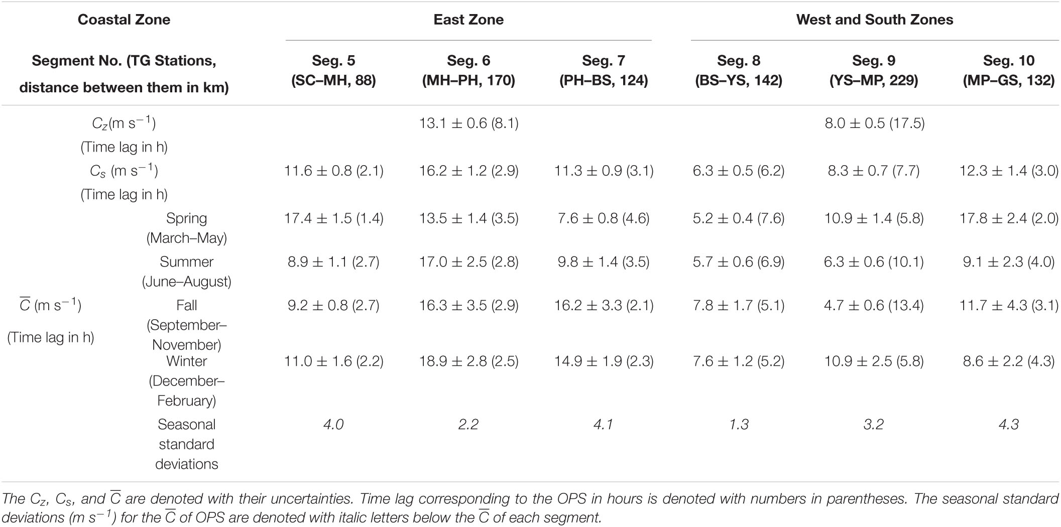
Table 1. C_z and C_s of the observed propagation speeds (OPS, m s^–1) in two coastal zones (East Zone, West and South zones collectively), for six segments (Segs. 5–10), and the $\overline{C}$ of the OPS for four seasons (spring, summer, fall, and winter) and six segments.

The vertical profiles of NIFS T and S were quality controlled and quality assured following (Bushnell and Worthington, 2016). First, outliers exceeding the global ranges of T (from −2.5 to 40°C) and S (from 2 to 41) were removed. Next, outliers exceeding three standard deviations from the monthly climatological mean of T (ranging from 0.2 to 33°C) and S (ranging from 27.1 to 35.7°C) at each station and depth were removed. Conservative temperature (T_C), absolute salinity (S_A), and the density (ρ) at the surface pressure (zero dbar) were calculated from NIFS T and S using the Gibbs Seawater Oceanographic Toolbox (McDougall and Barker, 2011). To prevent vertical density inversion, data with higher density at upper than lower depth levels were removed from the analysis. A vertical profile of the buoyancy frequency squared (N²) at each station was estimated using:

$N^2=-\frac{g}{{\mathrm{\rho }}_0}\frac{\partial \mathrm{\rho }}{\partial z}(3)$

All N² profiles were vertically interpolated at intervals of 1 m and were averaged over each season and segment. The N² derived from WOA18 data ($N_W^2$) were used as reference and compared with the N² derived from NIFS data $(N_{obs}^2$) for the same season and segment (Segs. 5–10); the difference was within 3% and quantified as $|1-N_W^2/N_{obs}^2|$. A few N² profiles averaged over each segment were used to represent N² profiles in the segment (Figures 2k–t).

To analyze the sea level response to (P − P₀), periods of strong and weak (τ^y) fluctuations were selected based on the variance averaged over the total period for the subtidal time scale using the MATLAB toolbox for wavelet analysis (Torrence and Compo, 1998). Periods of “weak” and “strong” fluctuations of atmospheric pressure were defined as the periods when the subtidal (P − P₀) variance was lower and higher than the temporal mean (= 0.25), respectively. In addition, the time-series of (P − P₀), η_obs, η_obs − η_IB, and η_obs − η_a (η_adj) were compared for 2-day-long periods for both weak (13–15 July 2007) and strong (22–24 March 2012) (P − P₀) fluctuations.

Wind-Forced CTW Model and Its Application

The cross-sectional modal structure (F), frictional decaying coefficient (a), wind coupling coefficient (b), and MPS (c) were computed using the wind-forced CTW model. For linear, hydrostatic, Boussinesq, f-plane, free-surface, and long wave approximations, the equation of motion can be solved by expanding the subsurface oceanic perturbation pressure, p, as a sum of modes. Here, the subsurface perturbation pressure corresponds to the pressure due to the adjusted (not observed) sea level (η_adj), i.e., p  =ρ₀gη_adj = ρ₀g(η_obs − η_a). To incorporate the non-isostatic sea level response to atmospheric pressure in the region, Eq. (2) instead of Eq. (1) was used in this study. Each mode contribution is a multiplication of the cross-sectional modal structure (F) and time- and alongshore varying amplitude (ϕ) as follows:

$p(x,y,z,t)=\sum _{n=1}^{\mathrm{\infty }}{F}_n(x,z){\mathrm{\varphi }}_n(y,t)(4)$

where z is the vertical coordinate, t is the time, and F_n is the normalized F of the n-th mode, which is weighted by the amplitude of the n-th mode CTWs, such that ϕ_n is as follows (Battisti and Hickey, 1984; Clarke and Van Gorder, 1986):

${\left({\mathrm{\varphi }}_n\right)}_y-c_n^{-1}{\left({\mathrm{\varphi }}_n\right)}_t+\sum _m{a}_{nm}{\mathrm{\varphi }}_m=b_n{\mathrm{\tau }}^y(y,t)(5)$

where a_nm is the frictional decay coefficient of the n-th mode to m-th mode, which is calculated as (Jordi et al., 2005; Cho et al., 2014):

$\begin{array}{c}{a}_{nm}=\frac{1}{f}\underset{0}{\overset{\mathrm{\infty }}{\int }}{F}_n(x,h){\left\{r{\left[F_m(x,h)\right]}_x\right\}}_{x}dx\hfill \\ +{\frac{1}{f}\underset{h}{\overset{0}{\int }}\frac{F_n(x,z){\left[F_m(x,z)\right]}_{x}r}{h\left(x\right)}|}_{x=0}dz\hfill \end{array}(6)$

where h(x) is the cross-shore profile of water depth across the segment, f is the Coriolis parameter at each latitude, and r is the bottom friction coefficient (Clarke and Van Gorder, 1986; Jordi et al., 2005; Cho et al., 2014). In Eq. (5), the b_n and c_n are the wind coupling coefficient and MPS of n-th mode CTWs, respectively, where b_n is calculated as follows (Jordi et al., 2005; Cho et al., 2014):

$b_n=\frac{1}{h\left(0\right)}\underset{h\left(0\right)}{\overset{0}{\int }}{F}_n(0,z)dz(7)$

The frictional decay coefficient a and wind coupling coefficient b represent the bottom stress of friction and surface wind stress associated with bottom topography and density stratification affecting the CTW propagation in a certain mode (Brink, 1982, 1991; Battisti and Hickey, 1984). The amplitude of mode-1 CTWs (ϕ₁) can be calculated, in an integrating form, as a function of the distance (y) from the origin (y = 0) and time (t) as follows (Battisti and Hickey, 1984; Clarke and Van Gorder, 1986):

$\begin{array}{c}{\mathrm{\varphi }}_1(y,t)={\mathrm{\varphi }}_1(0,t-\underset{0}{\overset{y}{\int }}{c}_1^{-1}d\xi )\exp \left(-\underset{0}{\overset{y}{\int }}{a}_{11}d\xi \right)\hfill \\ +\underset{0}{\overset{y}{\int }}{b}_1\left(\xi \right){\mathrm{\tau }}^y(\xi ,t-\underset{\xi }{\overset{y}{\int }}{c}_1^{-1}d{\xi }^{\prime })\hfill \\ \exp \left(-\underset{\xi }{\overset{y}{\int }}{a}_{11}d{\xi }^{\prime }\right)d\xi \hfill \end{array}(8)$

where the ϕ₁ at the origin (y = 0) was set to zero following previous studies on CTWs in the region (Cho et al., 2014; Park and Nam, 2018). This boundary condition is justified as the wind stresses at up-shelf grids around the origin was not large compared to those at down-shelf grids (e.g., W9, W18, and W32) so that inclusion of wind stresses at the up-shelf grids does not change the results significantly. The MATLAB code package “bigr.m” was used to calculate the CTW parameters (Brink, 2018). Multiple cross-shore profiles of bottom topography across the shelf within each segment and vertical N² profiles averaged over each segment area were used as the inputs for the CTW model to represent the topographic and stratification condition of the segment (Figure 2). Considering the assumption of alongshore uniformity for the CTW model, each segment was divided considering alongshore changes (in order of magnitude comparable to wavelength of the CTWs) in coastline direction, cross-shore shelf topography, and stratification. The applicability of the CTW theory assuming straight coastline and uniform along-shelf conditions was tested by comparing the results with observations. The f and r were fixed to constants of 8.803 × 10^–5 s^–1 and 0.005 cm s^–1, respectively (Cho et al., 2014). Results for the MPS were not sensitive (<1% change) to the selection of r in a reasonable range (from 0.005 to 0.1). The grid size was set to 100 (cross-shore) by 30 (vertical), and the width of the domain (maximum x) was set to 200 km, where the water depth was set to be constant for x > 100 km (seaward of the slope) (Cho et al., 2014).

Both OPS and MPS were averaged over each season, segment, and coastal zone (Tables 1, 2). The season-mean OPS and MPS ($\overline{C}$) were calculated based on data from the corresponding season over the total period of 21 years, namely 84 separate periods (21 years and four seasons). The segment-mean OPS and MPS (C_s) and coastal zone-mean speeds (C_z) were calculated based on data for corresponding seasons and segments, i.e., for 252 separate periods (21 years × 4 seasons × 3 segments) for each coastal zone. The mean speeds were obtained by weighted-averaging the OPS and MPS over the season, segment, and coastal zone, where the weights are derived from the maximum correlation coefficients among the TG sea level fluctuations. The $\overline{C}$ variability were quantified from interannual spreads using standard errors calculated as $\frac{\mathrm{\sigma }}{\sqrt{Y}}$ (σ: standard deviation of season-mean OPS and MPS in each year and Y is the number of samples set to 21). Similarly, variability in C_s and C_z was estimated based on the standard errors as $\frac{{\mathrm{\sigma }}^{\prime }}{\sqrt{Y^{\prime }}}$ [σ′: standard deviation of the segment-mean or coastal zone-mean OPS and MPS in each segment or coastal zone and Y′ is the number of samples set to 84 (segment-mean) or 252 (coastal zone-mean)].

TABLE 2

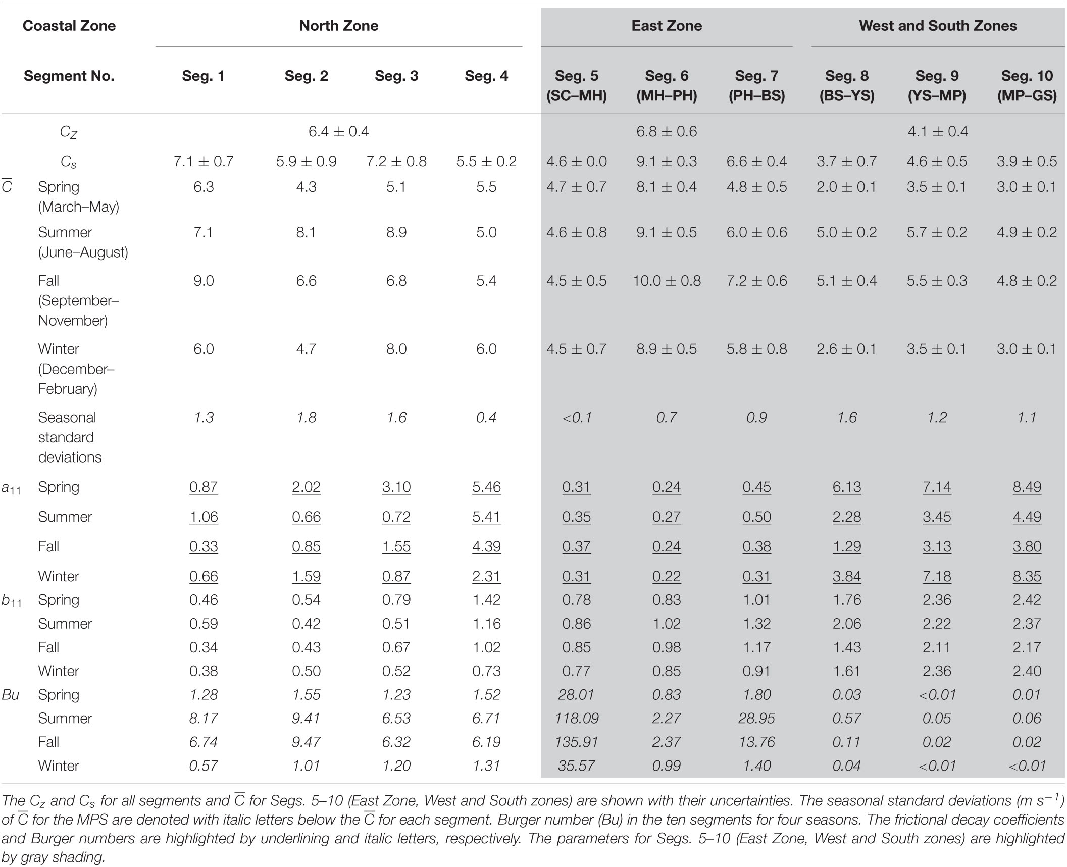
Table 2. C_z and C_s of the modeled phase speeds (MPS, c₁: m s^–1) of the first CTW mode (n = 1) in three coastal zones (North Zone, East Zone, West and South zones collectively) and for ten segments (Segs. 1–10), and the $\overline{C}$ of the MPS, frictional decay coefficients (a₁₁: 10^–9 cm^–1), and wind coupling coefficients (b₁: s^1/2 cm^–1/2) of the first CTW mode for four seasons (spring, summer, fall, and winter) and ten segments.

The CTW model results for four seasons and 10 segments were compared in terms of four parameters, estimated separately from the model: (1) Total water depth (H_i); (2) Shelf width (W_i) or the distance between the coastal wall and shelf break in segment C_s; (3) Vertical density difference (D_i,j) between the lower boundary of the seasonal thermocline (seasonal thermocline set to 70 m) and the bottom; and (4) Depth-averaged buoyancy frequency squared (M_i,j) for segment i and season j. These parameters were estimated to quantify the bottom topography and density stratification used as the model inputs, and to discuss the model results in this region in comparison to those in other regions. Here, the shelf break was defined as the location closest to the coastal wall where the bottom slope exceeds the mean bottom slope over the segment. The H_i and W_i are parameters characterizing shelf topography, whereas D_i,j and M_i,j are the stratification conditions, defined as:

$D_{i,j}=\frac{{\mathrm{\rho }}_0}{g}\underset{H_i}{\overset{70}{\int }}{N}_{i,j}^{2}dz(9)$

$M_{i,j}=\frac{1}{H_i}\underset{H_i}{\overset{0}{\int }}{N}_{i,j}^{2}dz(10)$

where $N_{i,j}^2$ is the buoyancy frequency squared (N²) averaged over segment i and season j. Note that D_i,j was calculated below d_th, i.e., the depth where the standard deviation of the alongshore-mean exceeds that of the season-mean N² (Figure 2t). The Burger number, $B{u}_{i,j}\equiv \frac{N_{i,j}^{2}h{\left(W_i\right)}^2}{f^2{W}_i^2}$, at the shelf break for each season and segment was estimated to diagnose the relative importance between stratification and bottom relief, e.g., CTWs are more baroclinic (barotropic) for Bu ≫ 1 (Bu ≪ 1).

Decomposition of Wind-Driven Coastal Sea Level

Subtidal coastal sea level variations modeled using the classic wind-forced CTW theory and local and remote wind forcing beyond CTW dynamics were assumed to be a linear sum of three components:

${\mathrm{\eta }}_{mod}={\mathrm{\eta }}_1+{\mathrm{\eta }}_2+{\mathrm{\eta }}_3(11)$

where η₁, η₂, and η₃ denote sea level fluctuations due to (1) The alongshore propagation of wind-forced CTWs, (2) Local upwelling/downwelling response to local alongshore wind stress, τ^y, and (3) Sea level set-up/set-down by cross-shore wind stress, τ^x, respectively. The CTW dynamics underlying η₁ are associated with the balances among the pressure gradient, bottom frictional stress, and surface wind stress in the alongshore direction, e.g., $fu=-\frac{1}{\mathrm{\rho }f}\frac{\partial p^2}{\partial x\partial t}-\frac{1}{\mathrm{\rho }}\frac{\partial p}{\partial y}+\frac{1}{\mathrm{\rho }}\frac{\partial ({\mathrm{\tau }}_s^y-{\mathrm{\tau }}_b^y)}{\partial z}$ where ${\mathrm{\tau }}_s^y$ and ${\mathrm{\tau }}_b^y$ are the alongshore surface wind stress and bottom frictional stress, respectively, and geostrophic balance in the cross-shore direction. The η₂ value was derived from dynamics distinctly different from the CTW dynamics where the alongshore balance between the alongshore Coriolis force (due to non-zero cross-shore currents) and alongshore surface wind stress via cross-shore Ekman transport, e.g., $fu=\frac{1}{\mathrm{\rho }}\frac{\partial {\mathrm{\tau }}_s^y}{\partial z}$, yielding alongshore current v as a time-integrated form of alongshore wind stress, along with the thermal wind relationship in the cross-shore direction. Details on the dynamics deriving η₂ are available from supporting information in Park and Nam (2018). The main difference between the dynamics of η₁ and η₂ is whether to allow the pressure gradient in the alongshore direction (η₁) or not (η₂), e.g., uniform pressure in the alongshore direction. Unlike the geostrophic balance (thermal-wind relationship) in cross-shore directions in the other two dynamics, the last term, η₃, is not derived from the cross-shore geostrophic balance but non-negligible cross-shore wind stress where coastal set-up (set-down) is associated with the balance among the cross-shore pressure gradient, cross-shore Coriolis force due to the alongshore current, and surface wind stress in the cross-shore direction, e.g., $-fv=-\frac{1}{\mathrm{\rho }}\frac{\partial p}{\partial x}+\frac{{\mathrm{\tau }}_s^x}{\mathrm{\rho }}$ (Liu and Weisberg, 2007). The η₃ dynamics yield subtidal fluctuations of barotropic and baroclinic currents and sea level set-up/set-down primarily by the cross-shore wind stress, and may play a role in certain conditions, as in Liu and Weisberg (2007). Alongshore propagations of the coastal set-up (set-down) sea level were assumed to be governed by the balance between the alongshore pressure gradient and bottom friction, following mode-1 CTW dynamics.

The η₁ was directly calculated from the output of the CTW model (mode-1 CTWs), i.e., the perturbation pressure, P₁(0) = F₁(0, z)ϕ₁(y, t), at the coastal wall (x = 0), as follows:

${\mathrm{\eta }}_1=\frac{{\int }_{h\left(0\right)}^0{P}_{1}dz}{{\mathrm{\rho }}_{0}g}(12)$

The η₂ can be estimated using the alongshore current (v) driven by the alongshore wind stress, based on Park and Nam (2018), expressed in the following form:

$v=\frac{{\int }_{{\mathrm{\delta }}_s}^0{N}^{2}dz}{{\mathrm{\rho }}_0{f}^2\mathrm{\Delta }{x}^2}\underset{0}{\overset{t}{\int }}{\mathrm{\tau }}^y\exp \left(-\frac{t-t_s}{T_d}\right)d{t}_s(13)$

and using the geostrophic balance in the cross-shore direction:

${\mathrm{\eta }}_2=-\frac{f\mathrm{\Delta }x}{g}v(14)$

where δ_s, Δx, and T_d are the maximum thickness of the upper layer in the two-layered system, the first baroclinic Rossby radius of deformation, and the time scale of the exponentially decaying wind stress, respectively. Here, Δx was defined as $\frac{1}{f}\underset{{\mathrm{\delta }}_s}{\overset{0}{\int }}Ndz$, and T_d was set to 24 h following Park and Nam (2018). Subtidal sea level fluctuations induced by alongshore propagations of both wind-forced mode-1 CTWs and local upwelling/downwelling response to alongshore winds are expressed as follows:

${\mathrm{\eta }}_{1,2}={\mathrm{\eta }}_1+{\mathrm{\eta }}_2(15)$

The propagation speed of subtidal η_1,2 fluctuations (MPS by η_1,2) was calculated using the same method applied to the OPS (those of η_adj) described in the previous section as the speed can be departed from c₁ due to the effects of local upwelling/downwelling dynamics (η₂) in response to alongshore wind varying along the coast, although the η₂ itself does not propagate along the coast (no alongshore pressure gradient). The local set-up/set-down of sea level due to cross-shore wind stress (${\mathrm{\eta }}_3^{\prime }$) is defined as follows Liu and Weisberg (2007):

${\mathrm{\eta }}_3^{\prime }=\underset{0}{\overset{X}{\int }}\frac{{\mathrm{\tau }}^x}{{\mathrm{\rho }}_{0}gh\left(x\right)}dx(16)$

where the cross-shore distance, X, for integrating the cross-shore wind stress was set to 100 km, matching the maximum distance within the segment; for example, between the coastal wall and offshore boundary. Then, η₃ was obtained in the same manner as Eq. (8) was applied to η₁, from the assumption that the alongshore propagation speed was the same as c₁, yielding:

${\mathrm{\eta }}_3=\sum _0^y{\mathrm{\eta }}_3^{\prime }(\xi ,t-\underset{\xi }{\overset{y}{\int }}{c}_1^{-1}d{\xi }^{\prime })\exp \left(-\underset{\xi }{\overset{y}{\int }}{a}_{11}d{\xi }^{\prime }\right)(17)$

The results of the comparisons between the remote alongshore wind stress (τ^y) and local sea levels (η_adj and η₁) and between the modeled (η₁, η₂, η₃, and η_mod) and observed sea levels (η_adj) were quantified using cross-correlation coefficients (R) and linear regression coefficients: slope (β) and intercept (α).

Results

Characteristics of Observed Sea Level Propagation

Subtidal η_adj fluctuations were found to propagate in the down-shelf direction from SC to GS [equatorward along the east coast of the East Zone (Segs. 5–7), westward along the south coast of the South Zone (Segs. 8–9), and poleward along the west coast of the West Zone (Seg. 10)], with speeds varying over seasons and segments around the KP (Figures 3, 4). For example, on April 4–7, 1999 (corresponding to spring), the subtidal η_adj fluctuations observed in SC on April 4 gradually propagated to GS (dotted line in Figure 3A). The propagation of subtidal η_adj fluctuations took 0.5 days from SC to BS (Segs. 5–7), propagating at a relatively high speed of 8.8 m s^–1 [=distance of 382 km (SC-BS) per 0.5 days], and 2.2 days from BS to GS (Segs. 8–10), propagating with a low speed of 2.6 m s^–1 [=503 km (BS–GS) per 2.2 days]. Other examples presented in June 1999 (corresponding to summer) showed different propagation speeds to each other even during the same season (thick solid vs. dashed lines in Figure 3B). For example, for June 25–26, 1999, the subtidal η_adj fluctuations observed in SC on June 25 propagated to GS with a relatively high-speed of 14.6 m/s [ = 885 km (SC–GS) per 0.7 days], indicative of much faster propagation, e.g., nearly synchronous fluctuations over the distance. However, a similar fluctuation propagated with a low speed on June 16–19, yielding 3.7 m s^–1 [=885 km (SC–GS) per 2.8 days], implying mixing of subtidal sea level fluctuations due to propagations of different kinds of waves. The time lags yielding the maximum correlation between η_adj at SC and those at other TG stations for each season generally increased with distance from SC to GS; the total time lags between SC and GS varied between seasons, namely 40 h in spring and 25 h in summer in 1999 (dashed lines in Figures 4A,B).

FIGURE 3

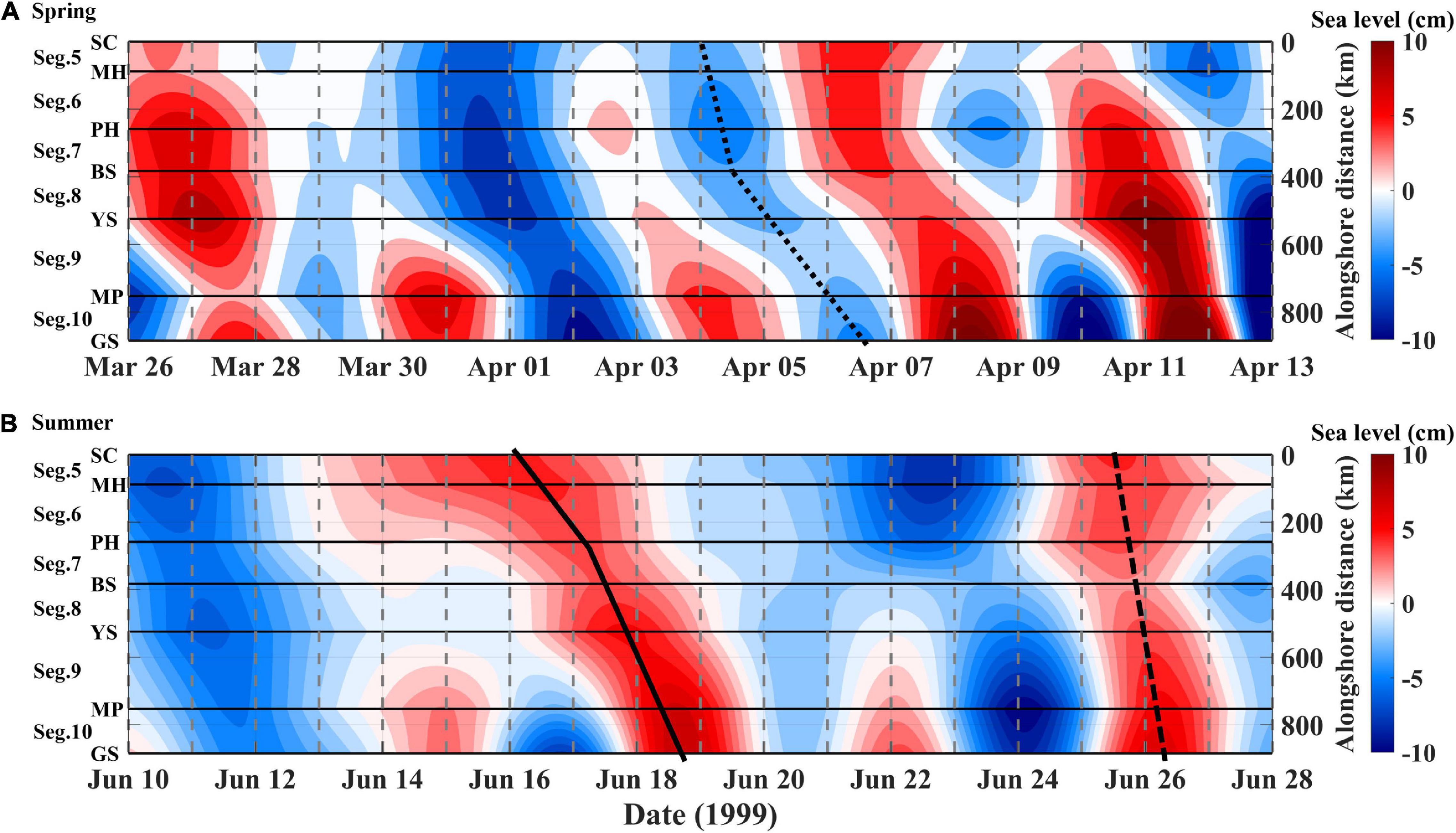
Figure 3. Hovmöller diagrams (x-axis: time, right y-axis: alongshore distance in km starting from SC to GS) for η_adj (colors with color bar on the right) around the KP for (A) spring and (B) summer of 1999. The selected events along the peaked sea level marked by a black-dotted line in (A) and by a black solid and dashed lines in (B) highlight clockwise propagation of subtidal sea level fluctuations around the KP. Corresponding segments and TG stations are noted with labels on the left y-axis and horizontal lines.

FIGURE 4

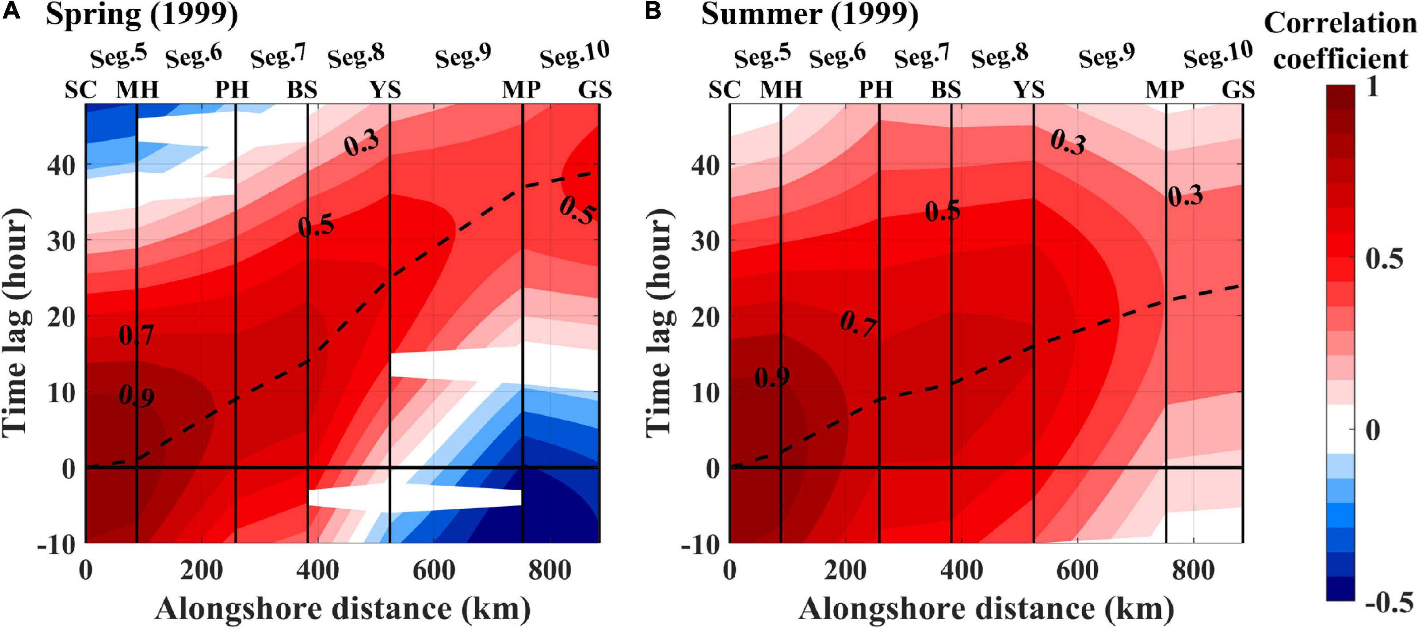
Figure 4. Cross-correlation coefficients (colors with label interval of 0.2) between η_adj at SC and those at seven TG stations along the coast around the KP for the (A) spring and (B) summer of 1999. Here, the x- and y-axis denote alongshore distance in km from SC toward GS and the time lag in hours, respectively. Corresponding segments and TG stations are denoted with labels on the top x-axis and vertical grid lines. The time lags at the maximum correlation are tracked and shown with dashed lines. The correlation coefficients not statistically significant at the 95% confidence level were discarded (blanked).

The η_adj propagated faster along the east coast (East Zone; Segs. 5–7) than along the west and south coasts (West and South zones; Segs. 8–10), yielding significantly higher C_z for the OPS of 13.1 ± 0.6 m s^–1 along the East Zone compared to that at 8.0 ± 0.5 m s^–1 along the West and South zones (Table 1). The C_s of the OPS reached a maximum speed of 16.2 ± 1.2 m s^–1 in Seg. 6, which was 41–46% higher than that in Seg. 5 (11.6 ± 0.8 m s^–1) and Seg. 7 (11.3 ± 0.9 m s^–1) and was statistically significant (Table 1 and Figure 5A). The C_s in Seg. 8 (6.3 ± 0.5 m s^–1) and 9 (8.3 ± 0.7 m s^–1) was significantly lower than those in other segments, and the minimum C_s among all of the segments occurred in Seg. 8. The C_s in Segs. 5, 7, and 10 (12.3 ± 1.4 m s^–1) were not significantly different from each other.

FIGURE 5

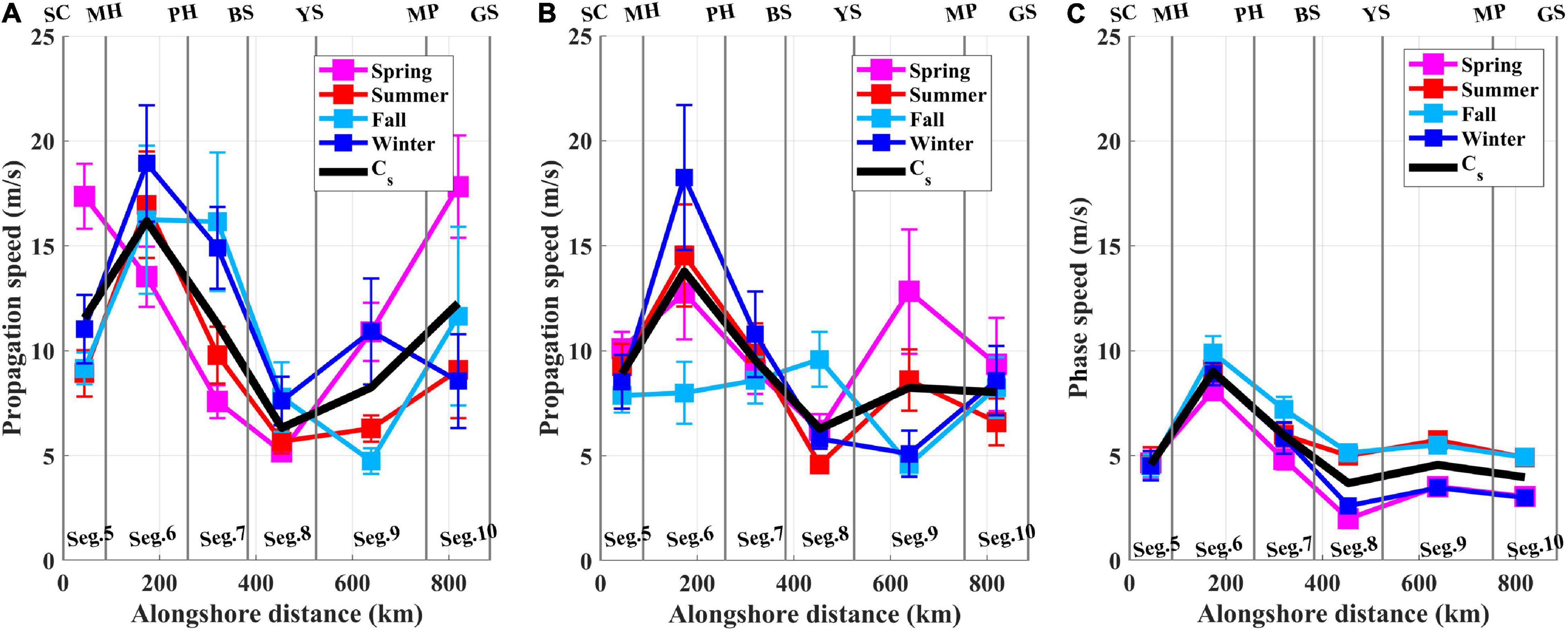
Figure 5. Segment-mean of the observed propagation speed (OPS) for each season ($\overline{C}$, y-axis) in m/s for (A) all periods, (B) only periods of weak subtidal fluctuations in atmospheric pressure (OPS-LP), and (C) the segment-mean of the modeled phase speed (MPS) of the mode-1 CTW (c₁) for each season ($\overline{C}$, y-axis) in m/s as a function of the alongshore distance in km (x-axis) for spring (pink squares and lines), summer (red squares and lines), fall (sky blue squares and lines), and winter (blue squares and lines), respectively. The season-mean of $\overline{C}$ (C_s) for the OPS and MPS in each segment is denoted by black solid lines. Vertical bars represent the uncertainties of the $\overline{C}$ estimation derived from the interannual spread.

Seasonal variations in the $\overline{C}$ of the OPS differed among the segments (Table 1 and Figure 5A). The $\overline{C}$ in spring was considerably higher in Segs. 5 (17.4 ± 1.5 m s^–1) and 10 (17.8 ± 2.4 m s^–1) by 57–98% and 42–164%, respectively, than the $\overline{C}$ in other seasons in each segment. In contrast, $\overline{C}$ in Segs. 6 (13.5 ± 1.4 m s^–1) and 7 (7.6 ± 0.8 m s^–1) showed the lowest speed in spring compared to those in other seasons. Seasonal variation in $\overline{C}$ in Seg. 8 was not significant. In Seg. 9, a higher $\overline{C}$ (by 79–137%) occurred in less stratified seasons (i.e., spring and winter) than in more stratified seasons (i.e., summer and fall).

Modeled Characteristics of Mode-1 CTW Propagation

A more baroclinic modal structure, F₁, smaller frictional decaying coefficient, a₁₁, smaller wind coupling coefficient, b₁, and higher MPS, c₁, were obtained along the east coast (East Zone) than along the west and south coasts of the KP (West and South zones), indicating significant alongshore variations in the CTW characteristics (Table 2 and Figure 5C). The C_z of the MPS was higher in the East Zone (6.8 ± 0.6 m s^–1) than in the West and South zones (4.1 ± 0.4 m s^–1) in a pattern similar to that in the observations (Table 2). The C_s of the MPS was highest in Seg. 6 (9.1 ± 0.3 m s^–1) and lowest in Seg. 8 (3.7 ± 0.7 m s^–1), which was also consistent with the observations (Table 2 and Figure 5C). In contrast, the C_s in Seg. 7 (6.6 ± 0.4 m s^–1) was 43% higher than in Seg. 5 (4.6 ± 0.0 m s^–1), unlike in the observations; this difference was statistically significant. The a₁₁ and b₁ were approximately 10- and 2-fold higher in the West and South zones than in the East Zone, respectively (Table 2). The F₁ was nearly baroclinic in the East Zone, yielding a Bu that generally exceeded unity, and more barotropic at the West and South zones with a relatively small Bu, particularly in spring and winter (Table 2 and Figure 6).

FIGURE 6

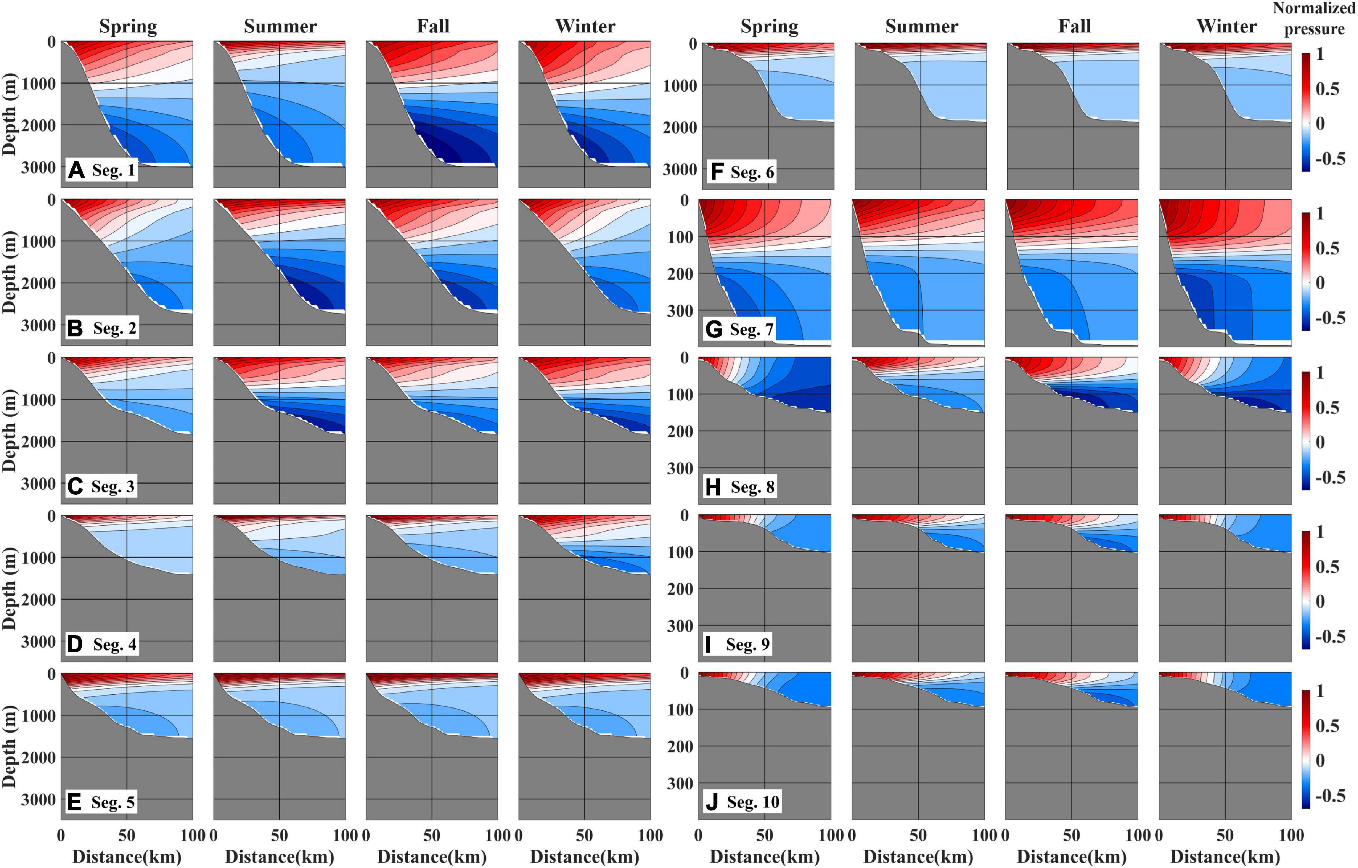
Figure 6. Cross-sectional modal structures (F₁) of the normalized pressure for the mode-1 CTWs in four seasons and ten segments (A–J). Water depth (y-axis) ranges from the surface to 3,500 m for Segs. 1–6 (A–F) and 400 m for Segs. 7–10 (G–J).

Seasonally, F₁ became more baroclinic with a smaller frictional decaying coefficient, a₁₁ and higher MPS, c₁ in summer and fall than in spring and winter, particularly in the West and South zones (Table 2 and Figure 5C). In contrast, wind coupling coefficient, b₁ was nearly constant (within 10%) over the seasons in the West and South zones. In the West and South zones, c₁ in summer and fall was 60–120% higher than that in spring and winter, indicating faster CTW propagation in the stratified seasons (Table 2 and Figure 5C). The seasonal standard deviations of c₁ were larger in the West and South zones (1.1–1.6 m s^–1) than in the East Zone (<0.9 m s^–1), implying that along the southern and western coasts of the KP, the CTWs were more sensitive to the seasonal variations of stratification (Table 2). The a₁₁ was also more sensitive to seasonal changes in stratification in the West and South zones (1.29–8.49 × 10^–9 cm^–1), where a₁₁ in summer and fall (1.29–4.49 × 10^–9 cm^–1) was half of that in spring and winter (3.84–8.49 × 10^–9 cm^–1), as compared to the East Zone (0.22–0.50 × 10^–9 cm^–1 within 16% variation; Table 2). The F₁ in the West and South zones demonstrated a more baroclinic structure in summer and fall with a relatively large Bu (0.02–0.57), whereas in spring and winter, the F₁ demonstrated a more barotropic structure with a small Bu (<0.04); however, such seasonal variation was not clear in the East Zone, which was nearly baroclinic in all seasons (Figure 6).

The modeled sea level in association with the mode-1 CTWs (η₁) propagated in the down-shelf direction from SC to GS around the KP. The modeled sea level η₁ had the highest correlation with the remote alongshore wind, τ^y, at W18, where the variance in the subtidal τ^y fluctuation was the largest among the three grids for wind stress (W9, W18, and W32; Table 3 and Figure 7). The RMS difference in alongshore wind at the three grids between CMEMS and MERRA2 for the total period from January 1997 to December 2017 is 3.4 m s^–1, which is less than the standard deviations of 4.8 m s^–1 (CMEMS) and 5.8 m s^–1 (MERRA2) for the same period. The correlation patterns between the modeled sea level η₁ at the TG stations and remote alongshore wind τ^y from the CMEMS wind products at the three grids were similar to those from the MERRA2 products (Table 3). Regardless of kinds of wind products, the modeled sea level was significantly correlated with remote alongshore winds. For example, the equatorward τ^y (downwelling favorable wind stress) at W18 on 20 and 24 September and 2 October led to drops in $\widetilde{{\mathrm{\eta }}_1}$ propagating from SC to GS around the KP (Figures 7A,B). From September to October 1999, η₁ at each TG station showed maximum correlation coefficients with τ^y, with the greatest among the three grids at W18 (0.47–0.87). The τ^y at W9 had a higher correlation coefficient (0.21–0.66) with η₁ at each TG station than τ^y at W32 (<0.22), despite the farther distance (Table 3).

TABLE 3

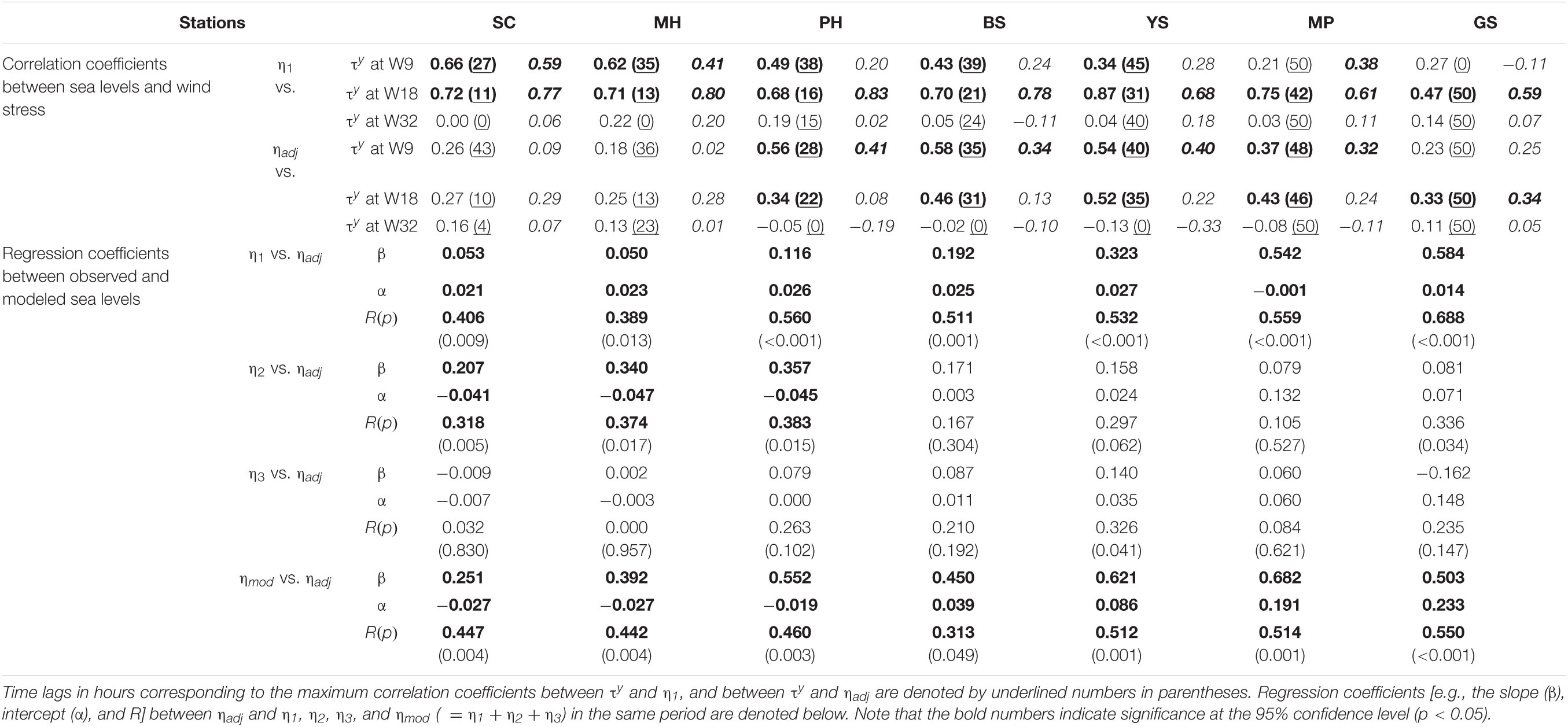
Table 3. Cross-correlation coefficients (Left: CMEMS satellite wind, Right in italics: MERRA2 reanalysis wind) between τ^y at three wind grids (τ^y at W9, W18, and W32) and η₁, and between τ^y at three wind grids and η_adj at each TG station from September 1 to October 30, 1999.

FIGURE 7

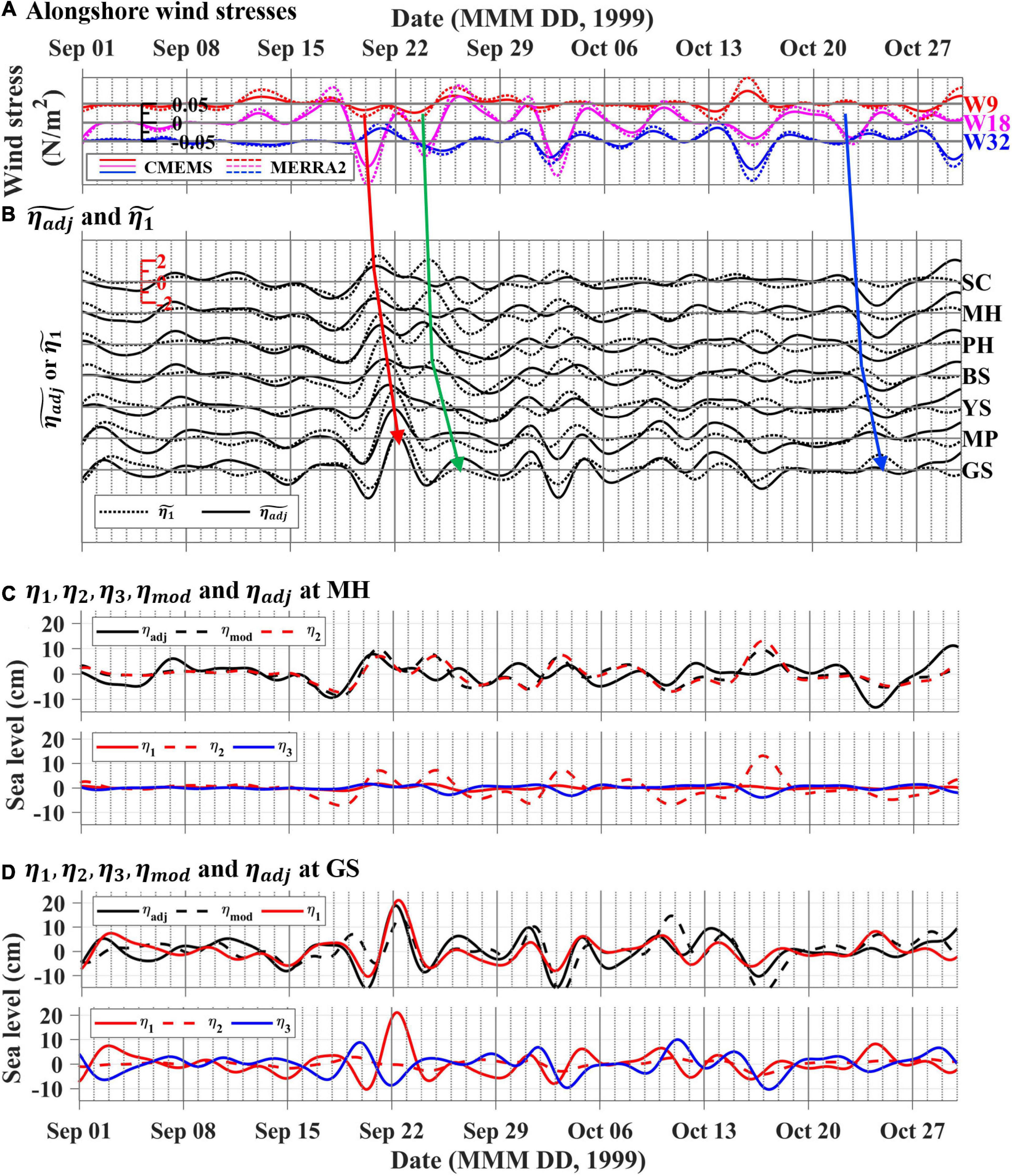
Figure 7. Time-series of (A) τ^y (colored solid lines for CMEMS blended satellite wind and colored dashed lines for the MERRA2 reanalysis wind) at three wind grids (W9, W18, and W32) located north of SC (colored squares in Figure 1), (B) $\widetilde{{\mathrm{\eta }}_{adj}}$ (solid line) and $\widetilde{{\mathrm{\eta }}_1}$ (dotted line) at the 7 TG stations 1 September to 30 October 1999. In (A,B), the propagations of η_adj and η₁, as well as the related τ^y described in section “Comparison Between Observed and Modeled Sea Level Propagations,” are highlighted by colored arrows. The time-series of η_adj and η_mod (=η₁ + η₂ + η₃) are shown at (C) MH and (D) GS. In the upper panel of (C,D), the η_adj and η_mod are represented by black solid and black-dashed lines, respectively. The η₂ (red-dashed line) and η₁ (red solid line), which are the most dominant at each station, were overlapped in the upper panels of (C,D), respectively. In the lower panels of (C,D), the red solid, red-dashed, and blue solid lines denote η₁, η₂, and η₃, respectively.

Comparison Between Observed and Modeled Sea Level Propagations

The CTW model systematically underestimated the propagation speed (i.e., MPS < OPS; Figures 5A,C). However, despite this systematic bias, common features were found in both OPS and MPS (c₁): C_z of OPS and MPS was consistently higher in the East Zone (Segs. 5–7) than in the West and South zones (Segs. 8–10). Overall, except for Seg. 10, the alongshore structures of C_s were consistent between the OPS and MPS. For example, both the OPS and MPS were the highest in Seg. 6, the second highest in Seg. 7, and the lowest in Seg. 8. However, the relatively high OPS in Seg. 10, which was similar to Segs. 5 and 7 in the East Zone, was not simulated by the CTW model. In addition, the C_s of OPS (6.3–16.2 m/s) was double that of the MPS (3.7–9.1 m/s) in all segments.

The seasonal variations in $\overline{C}$ of the MPS (c₁) showed higher speeds in summer and fall than in spring and winter, but were not clear in the $\overline{C}$ of the OPS (Figures 5A,C). Most seasonal variations in the $\overline{C}$ of the OPS and MPS were not consistent, except for the common low speed in spring in Segs. 6–7. In particular, the higher $\overline{C}$ of the OPS in spring (compared to other seasons) in Segs. 5 and 10 was not found in the MPS. The seasonal standard deviations of the $\overline{C}$ of the OPS (1.3–4.3 m/s) were substantially larger than those of the MPS (<1.6 m/s; Tables 1, 2).

Subtidal fluctuations in η₁ in each segment reconstructed by the mode-1 CTWs showed a significant correlation (0.39–0.69, p < 0.013) with those of η_adj observed at the corresponding TGs (Table 3). However, some sea level rises or drops in η_adj were not consistent with those in η₁, indicating that η_adj could not be solely explained by the mode-1 CTWs (Figure 7). For example, in both η_adj and η₁, the sea level rise on 20–22 September, which was led by downwelling favorable (equatorward) τ^y at W18, propagated sequentially from SC to GS (red arrows in Figures 7A,B). The sea level rise on October 23–24, which was led by downwelling favorable τ^y at W18 simulated by the model (η₁), was not observed in η_adj (blue arrows in Figures 7A,B). The sea level rise on September 24–26 in η₁, led by the τ^y at W18, was not observed at SC and MH, but at downstream TG stations from PH to GS (green arrows in Figures 7A,B). In addition, the subtidal fluctuations in η₁ were more correlated with η_adj at PH–GS (R between η₁ and η_adj: 0.511–0.688) than with those at SC (R between η₁ and η_adj: 0.406) and MH (R between η₁ and η_adj: 0.389).

Discussion

Effects of Mode-1 CTWs on Alongshore Propagation of η_adj

The shelf topography in each segment around the KP, which is characterized by water depth H and shelf width W, affected the propagation speed of the subtidal coastal sea level fluctuations, η_adj, around the KP. We observed higher speeds for wider W and deeper H, as is common in many coastal areas, e.g., areas off the west coast of the United States (Battisti and Hickey, 1984), west coast of Peru (Brink, 1982), and the South African coast (Schumann and Brink, 1990). The effects of the water depth on the MPS (c₁) were confirmed from the results, i.e., increasing with an increasing H and decreasing bottom frictional decay (smaller a₁₁) (Table 1 and Figures 5C, 8A). Interestingly, the OPS had a similar pattern to the MPS at higher propagation speeds at deeper depths (Tables 1, 2 and Figures 5A, 8A). In Segs. 5–7 (East Zone), where H was deeper than Segs. 8–10 (West and South zones), the overall OPS and MPS were relatively high (Tables 1, 2 and Figures 5A,C, 8A). The effects of the shelf width became clearer when comparing Seg. 5 (narrower shelf) and 6 (wider shelf) for a high H, and between Seg. 8 (narrower shelf) and 9 (wider shelf) for a low H. The c₁ increased with W, accounting for the higher OPS and MPS (c₁) in Seg. 6 and 9 when compared to Seg. 5 and 8, respectively (Tables 1, 2 and Figures 5A,C, 8B). In summary, despite the systematic underestimation (up to 60%) in the CTW model, the alongshore variations in the OPS were explained by the CTW dynamics affected by the shelf topography (H and W). However, since the OPS was also affected by the other kind of wave propagation, e.g., fast barotropic Kelvin waves yielding much higher propagation speed or nearly synchronous sea level response to atmospheric forcing (2nd event in Figure 3B), signal mixing with such processes beyond the CTW dynamics that is not incorporated into the CTW model may cause the model’s systematic underestimation (higher OPS than MPS).

FIGURE 8

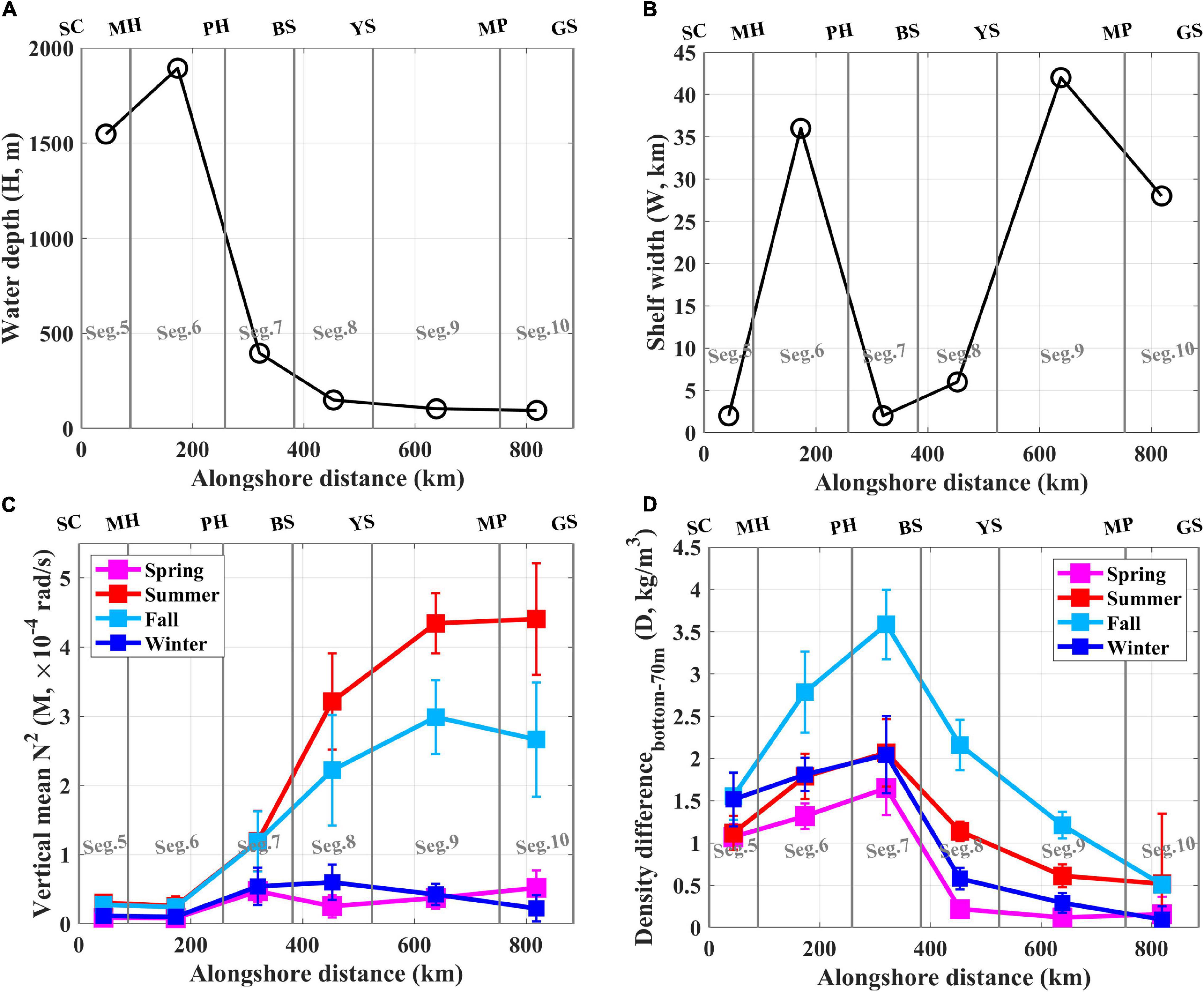
Figure 8. (A) Water depth (H) and (B) shelf width (W) as a function of the alongshore distance, (C) vertical mean N² (M), and (D) vertical density difference (D) between the bottom and the lower boundary of the seasonal thermocline (70 m) as a function of the alongshore distance for four seasons. For (C,D), vertical error bars denote the uncertainties over an interannual spread.

Density stratification, characterized by the vertical mean buoyancy frequency squared, M, and the density difference between the bottom and the lower boundary of the seasonal thermocline (d_th, 70 m), D, affects the MPS following mode-1 CTW dynamics; in other words, higher speeds with the stronger density stratification with larger D and M, but their effect on OPS was partial. This faster propagation of the CTWs by stronger seasonal stratification has been simulated in many studies, but has not yet been well observed (Wang and Mooers, 1976; Battisti and Hickey, 1984; Schumann and Brink, 1990; Brunner et al., 2019). Increasing stratification in summer and fall with the faster propagation of the CTWs is related to decreasing a₁₁, because the increased stratification mitigates the effect of bottom friction and wave damping (Brink, 1982, 1991). Although higher MPSs (c₁) were found with more stratified conditions, yielding a large D and M and small a₁₁, as suggested by previous studies (Wang and Mooers, 1976; Brink, 1991; Brunner et al., 2019), the greatest seasonal variations in the OPS could not be explained by the CTW dynamics (Tables 1, 2 and Figures 5A,C). However, the low $\overline{C}$ of the OPS in Segs. 6 and 7 in spring, consistent with the MPS, suggested that the seasonal variations in the OPS could also be partly affected by seasonal stratification; in other words, the smaller the D and M, the lower the OPS (Figures 5A, 8C,D). In contrast, the effect of vertical density differences between the bottom and d_th became clearer based on the comparison between the C_s in Segs. 5 and 7. The higher or similar C_s values of the OPS and MPS in Seg. 7, in comparison with Seg. 5, were due to the larger D in Seg. 7, despite the deeper water in Seg. 5 (Tables 1, 2 and Figures 5A,C, 8D). However, although a higher c₁ could be mainly explained by the stronger stratification with a larger M in Segs. 8–10 in summer and fall, the seasonal variations in the $\overline{C}$ of the OPS remain unclear. In summary, the CTW dynamics affected by the density stratification (D and M) partly accounted for both seasonal and alongshore variations in the OPS around the KP.

The MPSs around the KP reported in this study were not aligned with those found in other coastal regions, which is possibly due to distinctly different regimes in the shelf topography and density stratification, as compared with those of other studies. Relatively shallow water depth (small H) in the study area compared to those off the west coast of Peru (Brink, 1982; Illig et al., 2018) and the East Australian coast (Church et al., 1986; Figure 9) with no significant difference (slightly narrower) in shelf width W from those in other coastal areas (Figure 2a), cannot explain the faster propagating CTWs in the study region (with small H and W) than other regions (Figure 9). Note that the MPS generally decreased toward the left-bottom corner in Figure 9A, except for those found in this study. Thus, a striking difference in the stratification regime is responsible for the abnormal MPS in the study region. As the seawater that occupies below a depth of ∼100 m in the study region is cold (water temperature is less than 1°C) and nearly homogeneous (Kim et al., 2004), the N² is extremely small, as confirmed by the comparison of the vertical N² profiles in Seg. 1 to those off the west coast of Peru (Brink, 1982; Illig et al., 2018) and the East Australian coast (Church et al., 1986); however, strong seasonal variation in N² in the upper 100 m allows even higher stratification in the study region (Figure 2k). The stratification characterized by N² averaged over the upper 100 m yielded the distinctly different regimes from the other regions, accounting for the high MPS in the study region (Figures 9B,C).

FIGURE 9

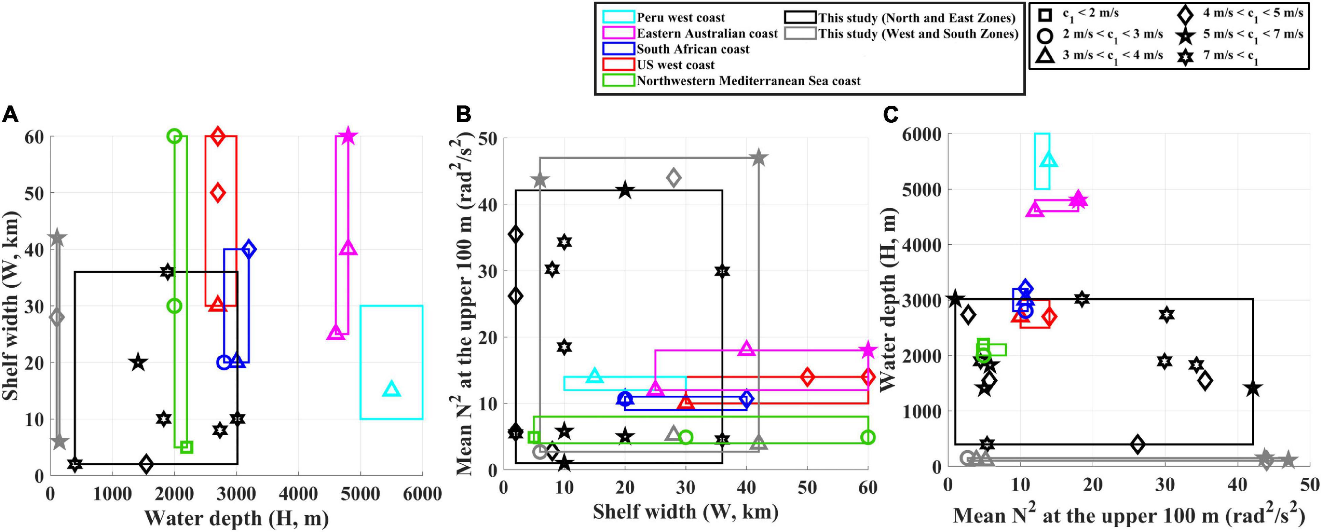
Figure 9. Comparison of mode-1 CTW phase speeds or MPS (range of c₁ denoted with symbols in the upper right box) derived from this (black: North and East Zones; gray: West and South Zones) and other studies (colors) as functions of the (A) water depth (H) and shelf width (W), (B) shelf width (W) and N² averaged (M) over the upper 100 m, and (C) N² averaged (M) over the upper 100 m and water depth (H). Studies on CTWs off the west coast of the United States (red) (Battisti and Hickey, 1984), South African coast (blue) (Schumann and Brink, 1990; Illig et al., 2018), west coast of Peru (cyan) (Brink, 1982; Illig et al., 2018), north-western Mediterranean Sea coast (green) (Jordi et al., 2005), and Eastern Australian coast (Church et al., 1986), are shown for comparison.

The correlation between η_adj and τ^y was higher at W18 than at W9 or W32, which demonstrates the importance of remote wind forcing and alongshore/temporal scales, relevant to the mode-1 CTWs, on the subtidal sea level fluctuations propagating around the KP (Table 3 and Figures 7A,B). Subtidal sea level fluctuations associated with remote wind forcing at locations separated by hundreds of kilometers, rather than local winds, following the dynamics of mode-1 wind-forced CTW, have been reported in this (Cho et al., 2014; Park and Nam, 2018) and other coastal areas (Battisti and Hickey, 1984; Clarke and Van Gorder, 1986). The subtidal sea level fluctuations along the entire coastline of the KP (1,830 km from Segs. 1 to 10) can be affected by alongshore wind forcing off the north coast (W9 and W18) following the dynamics of the mode-1 wind-forced CTW, considering the sufficiently long frictional damping length scales (Csanady, 1978; Park and Nam, 2018). The frictional damping length scales corresponding to frictional decay coefficients of 0.33–5.46 × 10^–9 cm^–1 for the North Zone (Table 2) is 1.8–30.3 × 10³ km, supporting the sensitivity of subtidal sea level fluctuations along the entire KP coast to alongshore wind off the north coast. The signal of subtidal sea level fluctuations generated by the alongshore wind forcing off the north coast would arrive in the west coast within a few days following the propagation speed of mode-1 CTWs. For example, for the distance from W18 to GS (1,330 km) and the C_s of c₁ in Segs. 3–10 (3.7–9.1 m s^–1), the sea level fluctuation led by τ^y at W18 arrived at GS within 1.7–4.2 days, which was confirmed by the propagation of the sea level fluctuations on September 20–22, 1999 (Figure 7B).

Effects of Wind and Atmospheric Forcing on Alongshore Propagation of η_adj

The subtidal fluctuations in the atmospheric pressure loading to the sea level over a large area with a minimized time lag could induce higher OPS beyond CTW dynamics, resulting in a systematically higher OPS than MPS. The subtidal fluctuations in the atmospheric pressure pattern around the KP are known to be mainly induced by the eastward movement of low pressure developed inland in Asia in spring and summer (Jung et al., 2008). As shown in the period of strong fluctuations in atmospheric pressure (March 22–24, 2012; Figures 10B–E), with variance higher (= 0.50) than the mean (= 0.25; Figure 10A), the eastward propagation of sea level fluctuations (from MP to PH; Figure 10C), induced by the pattern of eastward movement of subtidal fluctuations in atmospheric pressure (Figure 10B), remained stable after two different corrections (Figures 10D,E). In contrast, in the period of weak fluctuations in atmospheric pressure (July 13–15, 2007; Figures 10F–I), with variance lower than the mean (= 0.15; Figure 10A), the sea level fluctuations induced by the pattern of subtidal fluctuations in atmospheric pressure (Figure 10G) were removed, and the westward propagation of the sea level relevant to the propagation of the CTWs became distinct after corrections (Figures 10H,I). The C_s of the OPS based on η_adj, chosen only in periods of weak fluctuations in atmospheric pressure (OPS-LP), was smaller by 15 ± 13% than the C_s of the OPS based on the total η_adj (Figures 5A,B, 11A). In addition, the significantly higher $\overline{C}$ of the OPS at Segs. 5 and 10 in spring, which could not be accounted for by the MPS, disappeared in the $\overline{C}$ of the OPS-LP (Figure 5B). When the subtidal fluctuations in atmospheric pressure were strong, their loading effects on sea level would not optimally be removed by the corrections, such that they would increase the correlations between the sea level at adjacent TG stations by a similar pressure loading effect, yielding a larger OPS than the theoretical CTW phase speed.

FIGURE 10

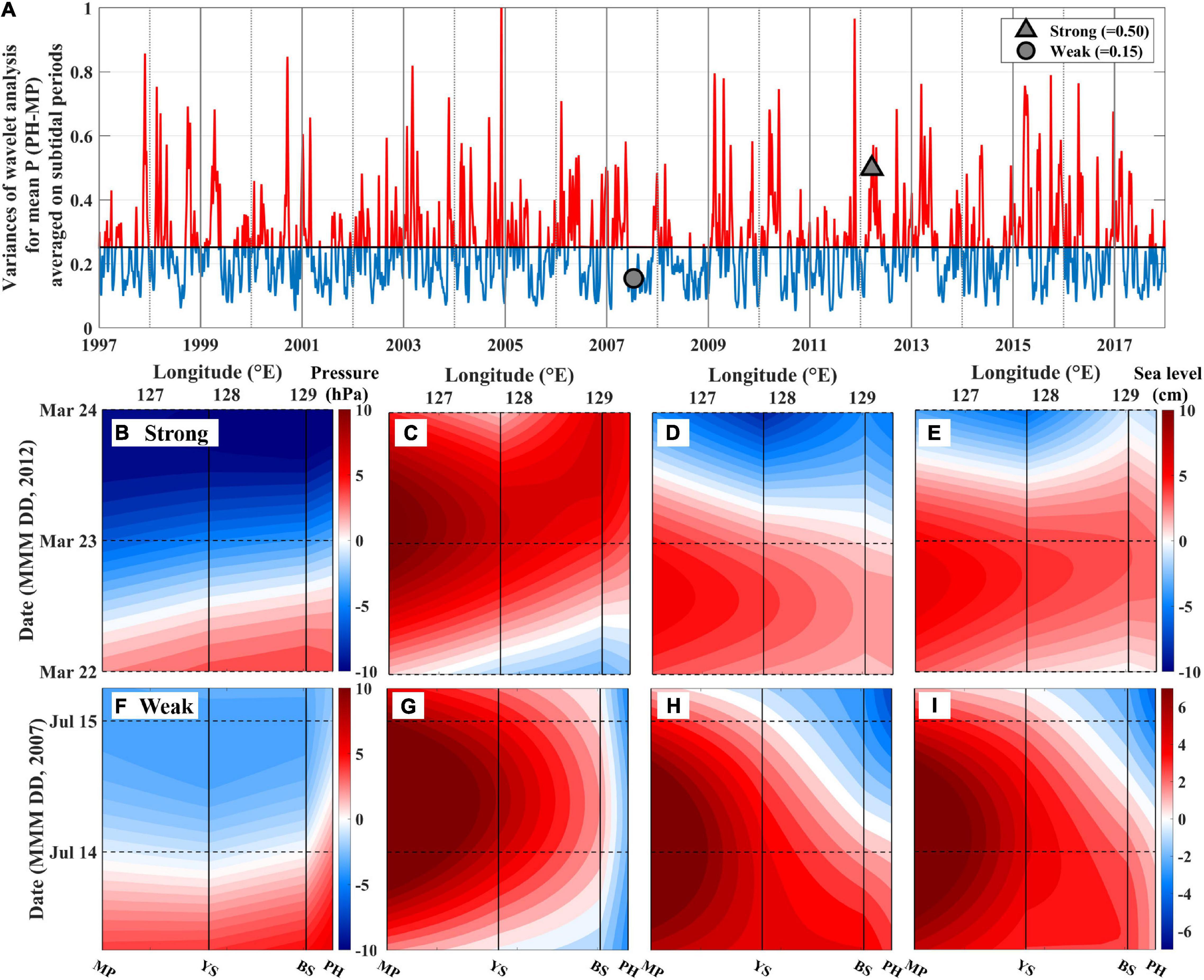
Figure 10. (A) Time-series of variance in the wavelet analysis for subtidal periods of atmospheric pressure fluctuations. The black solid line denotes the mean (= 0.25) of the variance of the total period, and the red and blue lines show the period with the stronger and weaker subtidal fluctuations in the atmospheric pressure than the mean value. The gray triangle and circle denote the events for the examples of strong (B–E) and weak (F–I) subtidal fluctuation in atmospheric pressure on the lower panels. Time-longitude patterns of (B,F) the atmospheric pressure anomaly and sea levels without (C,G) and with inverse barometric (D,H), and with the integrated response of non-isostatic and standard inverse barometric (E,I) corrections for the atmospheric pressure loading at four TG stations (MP, YS, BS, and PH).

FIGURE 11

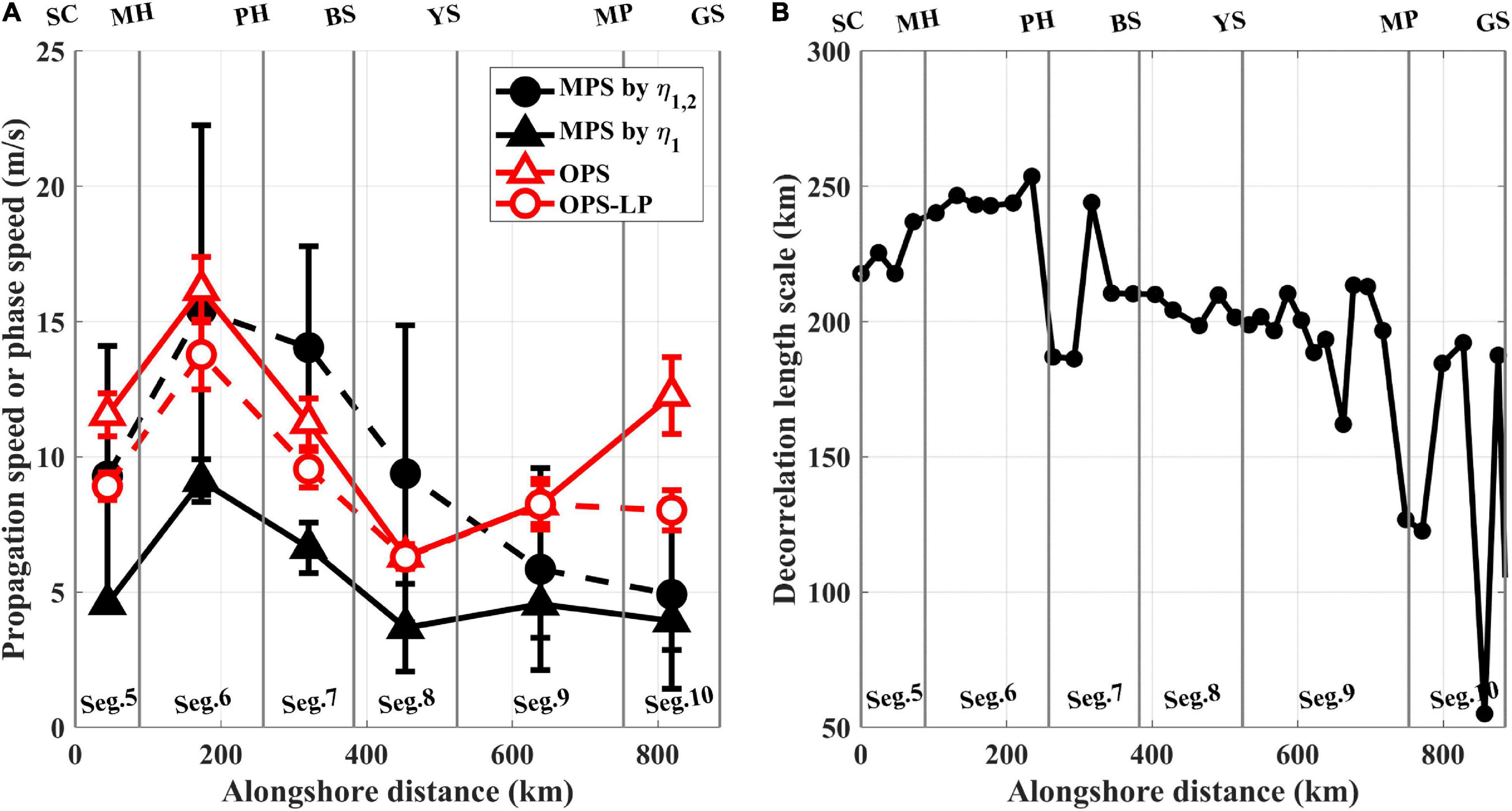
Figure 11. (A) C_s of MPS by η_1,2 (black circle and black-dashed line), MPS by η₁ (same as c₁, black triangle and black solid line), OPS (red triangle and red solid line), and OPS-LP (red circle and red-dashed line). (B) Decorrelation length scale of τ^y in SC–GS.

The upwelling/downwelling response of η_adj to the local τ^y could cause the systematically higher OPS (than MPS) by inducing a higher propagation speed with a minimized time lag due to the sufficiently large spatial (alongshore) scale of subtidal τ^y fluctuations (longer than the distance between neighboring TGs and comparable to the wavelength of mode-1 CTWs). The sea levels between neighboring TG stations responded almost simultaneously to the local τ^y; thus, inducing minimized time lags and higher propagation speeds. When considering both the upwelling/downwelling response to the local τ^y and mode-1 CTWs (MPS by η_1,2), the C_s of the MPS was 82 ± 50% larger than that of the MPS predicted by only η₁ (black-dashed and solid lines in Figure 11A). The upwelling/downwelling response of the sea level to the local τ^y was more significant in Segs. 5–8 than in Segs. 9–10, yielding a larger difference between the MPS by η_1,2 and MPS by η₁ in Segs. 5–8 due to the wider alongshore scales of the local τ^y, as confirmed by the longer decorrelation length scales of τ^y in Segs. 5–8 (Figure 11B).

Subtidal sea level fluctuations around the KP primarily induced by mode-1 CTWs (η₁) could be modified by the upwelling/downwelling response to local alongshore wind forcing (η₂) or local set-up/set-down of sea level due to cross-shore wind forcing (η₃), but the impacts varied among TG stations. The predominant η₂ was in SC–MH, the predominant η₁ was in BS-GS, and η₃ made the least contribution at all TG stations. The η₁ made the largest contribution to η_adj in BS–GS, as confirmed by the largest slopes ranging from 0.192 to 0.584 among all factors, as well as larger correlation coefficients between η₁ and η_adj in PH–GS when compared to those in SC–MH (Table 3 and Figures 7C,D). In contrast, η₂ had the greatest contribution to η_adj in SC–MH, with slopes ranging from 0.207 to 0.357 (Table 3 and Figure 7C). This result is consistent with the fact that the upwelling/downwelling response to local alongshore wind primarily explains the alongshore current variability at time scales shorter than approximately 16 days in the mid-east coast of South Korea (Park and Nam, 2018). The individual η₃ had the least contribution to η_adj (slope in the linear regression β of −0.162 to 0.140) at all TG stations among all components, along with a very low R (0.00–0.33); however, the sum of all of the components (η_mod), including η₃, better accounted for the subtidal sea level fluctuations in SC–MH (slope β of 0.251–0.682) than did any individual components, yielding a larger R (0.442–0.447) than any individual components (Table 3 and Figures 7C,D). The results reveal that the upwelling/downwelling response to local wind forcing plays a significant role in shaping subtidal sea level fluctuations around the KP beyond the wind-forced CTW dynamics where the time-varying wind forcing is considered with constant wind-coupling coefficient b.

Conclusion

Alongshore propagation in the down-shelf direction from SC to GS (equatorward along the east coast, westward along the south coast, and poleward along the west coast) around the KP of the coastal subtidal (3–20 days) sea level fluctuations were examined and modeled for mode-1 CTWs under varying shelf topographies and stratifications. In particular, alongshore and seasonal variations in the propagation speed were presented and discussed in terms of the dynamic response of the coastal sea level to atmospheric pressure and wind forcing (Figure 12A). The observed subtidal sea level fluctuations propagated with a higher speed of 13.1 ± 0.6 m s^–1 along the east coast (Segs. 5–7) and lower speed of 8.0 ± 0.5 m s^–1 along the west and south coasts (Segs. 8–10). This was similar to the alongshore variations of mode-1 CTWs (6.8 ± 0.6 m s^–1 along the east coast and 4.1 ± 0.4 m s^–1 along the west and south coasts), despite systematic underestimation by the CTW model that may be linked to dynamics beyond the wind-forced CTWs. The phase speeds of mode-1 CTWs increased with a deeper water depth, wider shelf width, and larger vertical density difference; these also accounted for most alongshore variations in the observed subtidal sea level propagation speeds around the KP (Figures 12B,C).

FIGURE 12

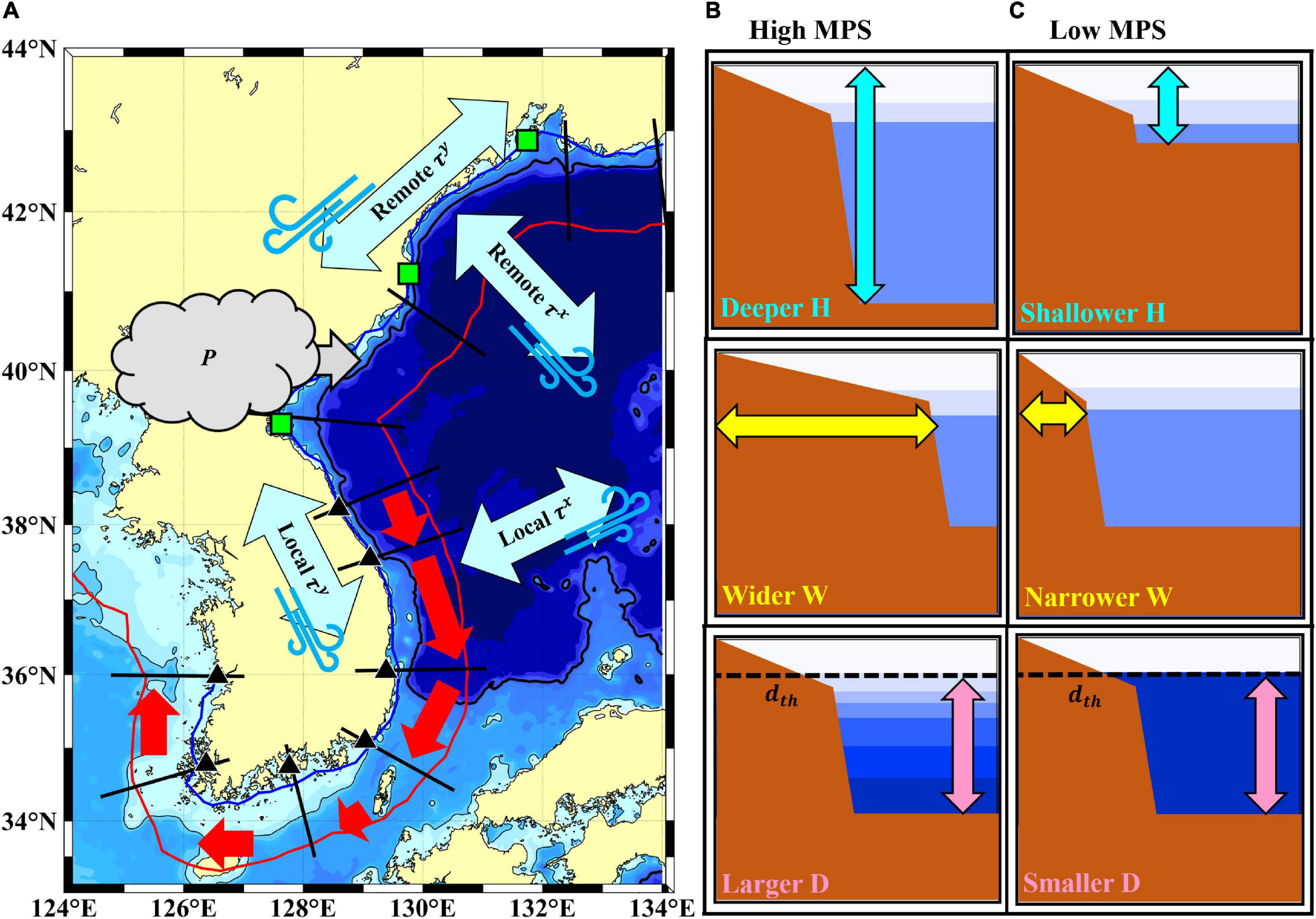
Figure 12. Schematic figures for the subtidal sea level fluctuation propagating around the KP and their relevant mechanisms. In the left panel (A), the causative forcing factors affecting the subtidal sea level fluctuation discussed in this study are denoted with gray (P, atmospheric pressure loading) and sky-blue arrows (τ^y and τ^x, alongshore and cross-shore wind forcing). The alongshore variations in the observed propagation speed of the subtidal sea level fluctuations are also represented with red arrows around the coastline of KP. In the right panels, the conditions for (B) the high MPS and (C) the low MPS following mode-1 CTWs dynamics are shown, i.e., water depth (H), shelf width (W), and the vertical density difference (D) between the lower boundary of the seasonal thermocline (d_th) and the bottom.

The barometric sea level response to the rapidly moving synoptic weather system and upwelling/downwelling response to local alongshore wind could account for the systematically higher propagation speeds of the observed sea level fluctuations. Subtidal sea level fluctuations around the KP were still affected by atmospheric pressure loading at the coastal sea level, which would not be fully corrected by known methods that consider the non-isostatic sea level response to atmospheric pressure in the semi-enclosed basin. Moreover, subtidal sea level fluctuations off the east coast beyond the CTW dynamics are partly explained by the upwelling/downwelling response to local (not remote) alongshore wind forcing, rather than the set-up/set-down response due to cross-shore wind forcing. The sufficiently larger alongshore scales of both the atmospheric pressure and local alongshore wind relative to distances among TG stations induced almost simultaneous sea level fluctuations at neighboring TG stations, thereby decreasing the time lags and deriving systematically higher propagation speeds. The atmospheric pressure loading, which would not be fully removed, may induce a 15% higher propagation speed, and the upwelling/downwelling response of coastal sea level to local alongshore wind may induce an 82% higher propagation speed for subtidal sea level fluctuations than that predicted by the CTW model. In addition to the previous works about the missing points of the classical CTW theory, including the complex coastline that may impact scattering of the CTWs (Huthnance et al., 1986; Jordi et al., 2005; Brunner et al., 2019), and non-linear advection that may hamper the model prediction (Cho et al., 2014), this study suggests the new point of subtidal coastal sea level fluctuations, particularly within semi-enclosed marginal seas: (1) Non-isostatic sea level response to atmospheric pressure loading and (2) Upwelling/downwelling response to local wind forcing play an important role in shaping the subtidal sea level fluctuations beyond the CTW theory.

Data Availability Statement

The TG station data were provided by the Korea Hydrographic and Oceanographic Administration (KHOA) and are available at https://www.khoa.go.kr/koofs. The ship-based hydrographic data were provided by the National Institute of Fisheries Science (NIFS) and are available at https://www.nifs.go.kr/kodc/. The sea surface pressure data were provided by the Korea Meteorological Administration (KMA) and are available at https://data.kma.go.kr/cmmn/main.do. The bottom topography data were from ETOPO2 (Earth topography 2 arc-minute) data provided by the US National Geophysical Data Center and are available at https://www.ngdc.noaa.gov/mgg/global/etopo2.html. The monthly climatology data were provided by WOA18 (World Ocean Atlas 2018) and are available at https://www.nodc.noaa.gov/OC5/woa18/. The blended wind stress data were provided by the Copernicus Marine Environment Monitoring Service (CMEMS) and are available at https://marine.copernicus.eu/services-portfolio/access-to-products. The reanalysis wind stress data were provided from the Modern-Era Retrospective Analysis, version-2 (MERRA-2) and are available at https://gmao.gsfc.nasa.gov/reanalysis/MERRA-2/.

Author Contributions

KL and SN contributed to conception of the study. KL organized the methodology, software, performed the formal analysis, visualized all of the figures, and wrote the original draft of the manuscript. KL, SN, and J-HP investigated the formally analyzed data and contributed to writing–review and editing. SN supervised all processes. All authors contributed to the manuscript in multiple ways.

Funding

This study was also a part of the project titled, “Deep Water Circulation and Material Cycling in the East Sea (20160040),” funded by the Ministry of Oceans and Fisheries (MOF), South Korea. This study was funded by the KHOA, MOF, through a project named titled, “Analysis and Prediction of Sea Level Change in Response to Climate Change around the Korean Peninsula.”

Conflict of Interest

The authors declare that the research was conducted in the absence of any commercial or financial relationships that could be construed as a potential conflict of interest.

Publisher’s Note

All claims expressed in this article are solely those of the authors and do not necessarily represent those of their affiliated organizations, or those of the publisher, the editors and the reviewers. Any product that may be evaluated in this article, or claim that may be made by its manufacturer, is not guaranteed or endorsed by the publisher.

Acknowledgments

The authors thank the two reviewers for their constructive suggestions to improve the quality of this manuscript and C. B. Cho for technical help in applying the CTW model. The MATLAB version of the CTW model package, generously provided by K. H. Brink, was used. The authors also thank Editage (www.editage.co.kr) for English language editing.

Supplementary Material

The Supplementary Material for this article can be found online at: https://www.frontiersin.org/articles/10.3389/fmars.2021.802752/full#supplementary-material

References

Amol, P., Shankar, D., Aparna, S. G., Shenoi, S. S. C., Fernando, V., Shetye, S. R., et al. (2012). Observational evidence from direct current measurements for propagation of remotely forced waves on the shelf off the west coast of India. J. Geophys. Res. Oceans 117:5017. doi: 10.1029/2011JC007606

CrossRef Full Text | Google Scholar

Battisti, D. S., and Hickey, B. M. (1984). Application of remote wind-forced coastal trapped wave theory to the Oregon and Washington coasts. J. Phys. Oceanogr. 14, 887–903. doi: 10.1175/1520-0485(1984)014<0887:AORWFC>2.0.CO;2

CrossRef Full Text | Google Scholar

Bentamy, A. (2019). Quality Information Document for the Global Ocean Wind Products WIND_GLO_WIND_L4_NRT_OBSERVATIONS_012_004. Available online at: https://paperzz.com/doc/7686602/quality-information-document-for-the-global-ocean-wind (accessed December 25, 2021).

Google Scholar

Bentamy, A., Grodsky, S. A., Cambon, G., Tandeo, P., Capet, X., Roy, C., et al. (2021). Twenty-seven years of scatterometer surface wind analysis over eastern boundary upwelling systems. Remote Sens. 13:940. doi: 10.3390/rs13050940

CrossRef Full Text | Google Scholar

Brink, K. H. (1982). A comparison of long coastal trapped wave theory with observations off Peru. J. Phys. Oceanogr. 12, 897–913. doi: 10.1175/1520-0485(1982)012<0897:ACOLCT>2.0.CO;2

CrossRef Full Text | Google Scholar

Brink, K. H. (1991). Coastal-trapped waves and wind-driven currents over the continental shelf. Annu. Rev. Fluid Mech. 23, 389–412. doi: 10.1146/annurev.fl.23.010191.002133

CrossRef Full Text | Google Scholar

Brink, K. H. (2018). Stable Coastal-Trapped Waves with Stratification, Topography and Mean Flow. Available online at: https://hdl.handle.net/1912/10527 (accessed October 26, 2021).

Google Scholar

Brunner, K., Rivas, D., and Lwiza, K. M. M. (2019). Application of classical coastal trapped wave theory to high-scattering regions. J. Phys. Oceanogr. 49, 2201–2216. doi: 10.1175/jpo-d-18-0112.1

CrossRef Full Text | Google Scholar

Bushnell, M., and Worthington, H. (2016). Manual for Real-Time Quality Control of in-Situ Temperature and Salinity Data: A Guide to Quality Control and Quality Assurance for In-Situ Temperature and Salinity Observations. Washington, DC: NOAA.

Google Scholar

Cho, C.-B., Nam, S., and Chang, K.-I. (2014). Subtidal temperature variability in stratified shelf water off the mid-east coast of Korea. Cont. Shelf Res. 75, 41–53. doi: 10.1016/j.csr.2013.12.011

CrossRef Full Text | Google Scholar

Church, J. A., Freeland, H. J., and Smith, R. L. (1986). Coastal-trapped waves on the East Australian continental shelf: Part I: propagation of modes. J. Phys. Oceanogr. 16, 1929–1943. doi: 10.1175/1520-0485(1986)016<1929:CTWOTE>2.0.CO;2

CrossRef Full Text | Google Scholar

Clarke, A. J., and Van Gorder, S. (1986). A method for estimating wind-driven frictional, time-dependent, stratified shelf and slope water flow. J. Phys. Oceanogr. 16, 1013–1028. doi: 10.1175/1520-0485(1986)016<1013:AMFEWD>2.0.CO;2

CrossRef Full Text | Google Scholar

Codiga, D. L. (2011). Unified Tidal Analysis and Prediction Using the UTide Matlab Functions. Technical Report 2011-01. (Narragansett, RI: University of Rhode Island), 59.

Google Scholar

Csanady, G. (1978). The arrested topographic wave. J. Phys. Oceanogr. 8, 47–62. doi: 10.1175/1520-0485(1978)008<0047:TATW>2.0.CO;2

CrossRef Full Text | Google Scholar

Gelaro, R., McCarty, W., Suárez, M. J., Todling, R., Molod, A., Takacs, L., et al. (2017). The Modern-Era retrospective analysis for research and applications, Version 2 (MERRA-2). J. Clim. 30, 5419–5454. doi: 10.1175/JCLI-D-16-0758.1

PubMed Abstract | CrossRef Full Text | Google Scholar

Hughes, C. W., Fukumori, I., Griffies, S. M., Huthnance, J. M., Minobe, S., Spence, P., et al. (2019). Sea level and the role of coastal trapped waves in mediating the influence of the open ocean on the coast. Surv. Geophys. 40, 1467–1492. doi: 10.1007/s10712-019-09535-x

CrossRef Full Text | Google Scholar

Huthnance, J. M. (1978). On coastal trapped waves: analysis and numerical calculation by inverse iteration. J. Phys. Oceanogr. 8, 74–92. doi: 10.1175/1520-0485(1978)008<0074:OCTWAA>2.0.CO;2

CrossRef Full Text | Google Scholar

Huthnance, J. M., Mysak, L. A., and Wang, D. P. (1986). “Coastal trapped waves,” in Baroclinic Processes on the Continental Shelves, ed. C. N. K. Mooers (Washington, DC: American Geophysical Union), 1–18. doi: 10.1029/CO003p0001

CrossRef Full Text | Google Scholar

Illig, S., Cadier, E., Bachèlery, M. L., and Kersalé, M. (2018). Subseasonal coastal-trapped wave propagations in the southeastern Pacific and Atlantic Oceans: 1. A new approach to estimate wave amplitude. J. Geophys. Res. Oceans 123, 3915–3941. doi: 10.1029/2017JC013539

CrossRef Full Text | Google Scholar

Inazu, D., Hirose, N., Kizu, S., and Hanawa, K. (2006). Zonally asymmetric response of the Japan Sea to synoptic pressure forcing. J. Oceanogr. 62, 909–916. doi: 10.1007/s10872-006-0108-9

CrossRef Full Text | Google Scholar

Jordi, A., Orfila, A., Basterretxea, G., and Tintoré, J. (2005). Coastal trapped waves in the northwestern Mediterranean. Cont. Shelf Res. 25, 185–196. doi: 10.1016/j.csr.2004.09.012

CrossRef Full Text | Google Scholar

Jung, S.-Y., Yun, J.-Y., Park, T.-W., Lim, S.-H., and Oh, I.-S. (2008). Sea level variability at a synoptic band along the east coast of Korea and its causal mechanism. Sea 13, 89–105.

Google Scholar

Kim, K., Kim, K. R., Kim, Y. G., Cho, Y. K., Kang, D. J., Takematsu, M., et al. (2004). Water masses and decadal variability in the East Sea (Sea of Japan). Prog. Oceanogr. 61, 157–174. doi: 10.1016/j.pocean.2004.06.003

CrossRef Full Text | Google Scholar

Lee, J., and Chung, J. (1982). Continental shelf waves off the eastern coast of Korea. Sea 20, 169–180.

Google Scholar

Liu, Y., and Weisberg, R. H. (2007). Ocean currents and sea surface heights estimated across the West Florida shelf. J. Phys. Oceanogr. 37, 1697–1713. doi: 10.1175/JPO3083.1

CrossRef Full Text | Google Scholar

Lyu, S. J., Kim, K., and Perkins, H. T. (2002). Atmospheric pressure-forced subinertial variations in the transport through the Korea Strait. Geophys. Res. Lett. 29, 8-1–8-4. doi: 10.1029/2001GL014366

CrossRef Full Text | Google Scholar

McDougall, T. J., and Barker, P. M. (2011). Getting started with TEOS-10 and the Gibbs Seawater (GSW) Oceanographic Toolbox. SCOR/IAPSO WG. 127, 1-28, ISBN 978-0-646-55621-5. Available online at: http://www.teos-10.org/pubs/Getting_Started.pdf (accessed December 25, 2021).

Google Scholar

Nam, S., Kim, Y. H., Park, K. A., and Kim, K. (2005). Spatio-temporal variability in sea surface wind stress near and off the east coast of Korea. Acta Oceanol. Sin. 24, 107–114.

Google Scholar

Nam, S. H., Lyu, S. J., Kim, Y. H., Kim, K., Park, J.-H., and Watts, D. R. (2004). Correction of TOPEX/POSEIDON altimeter data for nonisostatic sea level response to atmospheric pressure in the Japan/East Sea. Geophys. Res. Lett. 31:L02304. doi: 10.1029/2003GL018487

CrossRef Full Text | Google Scholar

Park, J.-H., and Nam, S. (2018). Causes of interannual variation of summer mean alongshore current near the east coast of Korea derived from 16-year-long observational data. J. Geophys. Res. Oceans 123, 7781–7794. doi: 10.1029/2018JC014053

CrossRef Full Text | Google Scholar

Schlosser, T. L., Jones, N. L., Musgrave, R. C., Bluteau, C. E., Ivey, G. N., and Lucas, A. J. (2019). Observations of diurnal coastal-trapped waves with a thermocline-intensified velocity field. J. Phys. Oceanogr. 49, 1973–1994. doi: 10.1175/JPO-D-18-0194.1

CrossRef Full Text | Google Scholar

Schumann, E., and Brink, K. (1990). Coastal-trapped waves off the coast of South Africa: generation, propagation and current structures. J. Phys. Oceanogr. 20, 1206–1218. doi: 10.1175/1520-0485(1990)020<1206:CTWOTC>2.0.CO;2

CrossRef Full Text | Google Scholar

Stammer, D., Cazenave, A., Ponte, R. M., and Tamisiea, M. E. (2013). Causes for contemporary regional sea level changes. Annu. Rev. Mar. Sci. 5, 21–46. doi: 10.1146/annurev-marine-121211-172406

PubMed Abstract | CrossRef Full Text | Google Scholar

Torrence, C., and Compo, G. P. (1998). A practical guide to wavelet analysis. Bull. Am. Meteorol. Soc. 79, 61–78. doi: 10.1175/1520-0477(1998)079<0061:APGTWA>2.0.CO;2

CrossRef Full Text | Google Scholar

Wang, D.-P., and Mooers, C. N. (1976). Coastal-trapped waves in a continuously stratified ocean. J. Phys. Oceanogr. 6, 853–863. doi: 10.1175/1520-0485(1976)006<0853:CTWIAC>2.0.CO;2

CrossRef Full Text | Google Scholar

Wunsch, C., and Stammer, D. (1997). Atmospheric loading and the oceanic “inverted barometer” effect. Rev. Geophys. 35, 79–107. doi: 10.1029/96RG03037

CrossRef Full Text | Google Scholar