Application of Non-stationary Extreme Value Analysis to Satellite-Observed Sea Surface Temperature Data for Past Decades

Extreme value analysis (EVA) has been extensively used to understand and predict long-term return extreme values. This study provides the first approach to EVA using satellite-observed sea surface temperature (SST) data over the past decades. Representative EVA methods were compared to select an appropriate method to derive SST extremes of the East/Japan Sea (EJS). As a result, the peaks-over-threshold (POT) method showed better performance than the other methods. The Optimum Interpolation Sea Surface Temperature (OISST) database was used to calculate the 100-year-return SST values in the EJS. The calculated SST extremes were 1.60–3.44°C higher than the average value of the upper 5th-percentile satellite-observed SSTs over the past decades (1982–2018). The monthly distribution of the SST extremes was similar to the known seasonal variation of SSTs in the EJS, but enhanced extreme SSTs exceeding 2°C appeared in early summer and late autumn. The calculated 100-year-return SSTs were compared with the simulation results of the Coupled Model Intercomparison Project 5 (CMIP5) climate model. As a result, the extreme SSTs were slightly smaller than the maximum SSTs of the model data with a negative bias of –0.36°C. This study suggests that the POT method can improve our understanding of future oceanic warming based on statistical approaches using SSTs observed by satellites over the past decades.

Introduction

Global warming and climate change have become widespread over time. In addition to the warming air temperature and land surface, the upper-ocean temperature of the global ocean has also increased over the past decades (Baker et al., 2004; Sutton et al., 2007; Stott, 2016). Along with the warming of the global ocean, regional seas have also experienced significant warming at significant rates (IPCC Climate Change, 2014). The influence of warming has induced more pronounced climate extremes.

As the scale of warming increases, the possibility of coastal disasters is also steadily growing (IPCC Climate Change, 2014; Stott, 2016). Therefore, it is necessary to predict the magnitude of such warming along with the extremes of sea surface temperatures (SSTs). Most of our understanding of ocean warming in the future depends on the simulation results using several numerical models. Several scenarios have been presented by adopting numerical model simulations under different conditions (e.g., Kharin et al., 2007; Sutton et al., 2007; IPCC Climate Change, 2014). The extreme temperatures were inferred from the results of the scenarios. Additionally, other approaches are also required to infer the extreme temperatures, not by numerical model results, but by long-term measurements. Satellite-observed SSTs have long been used to predict forward extreme temperatures.

In order to reduce the computation time of the model prediction and enhance the efficiency, extreme value analysis (EVA) has been proposed as a method to predict the extreme values. The EVA is a method that can predict the long-period return extreme values (e.g., 100-year-return extreme) by using observed values (Gumbel, 1958; Mearns et al., 1984; Wigley, 1985, 2009; Katz and Brown, 1992; Coles, 2001). This method has been widely used in the field of surface wave height (SWH) and wind speed (WS) (Mathiesen et al., 1994; Soares and Scotto, 2001, 2004; Caires and Sterl, 2005; Jonathan and Ewans, 2007; Martucci et al., 2010; Young et al., 2012). Caires and Sterl (2005) calculated 100-year SWH and WS by applying the peaks-over-threshold (POT) method to 40-year reanalysis data (ERA-40), and compared the results with buoy and altimeter data. Young et al. (2012) applied the initial distribution method (IDM) to altimeter data collected for the period over 20 years and computed the 100-year SWH and WS for four different periods between 1992 and 2008. The 100-year WS showed a positive trend, but the 100-year SWH showed no distinct trend. Notably, the significance of the computed value needs to be ensured for observation data over longer periods. The EVA method has not only been used for SWH and WS, but also for other marine fields such as rainfall (flood) (Cheng and AghaKouchak, 2014; Cheng et al., 2014). The results obtained through EVA predict extreme values that can be observed within a specific period (e.g., 100 years) and have also been utilized for diverse applications such as construction.

Studies have also been conducted for the computation of extreme surface air temperature (SAT) with EVA (Laurent and Parey, 2007; Parey et al., 2007; Coelho et al., 2008). The POT method to be applied to the SAT data was summarized by Parey et al. (2007) for computing the 100-year SAT using the temperature observation data for each station in France (Laurent and Parey, 2007). A similar approach to understand extreme values of the temperature field was extended to global regions using the POT method (Coelho et al., 2008). In contrast, EVA analysis has not been actively applied to SST fields in the ocean and remains in the testing phase (Coelho et al., 2008; Huser, 2021). It is highly possible and necessary to apply the POT method to the oceanic temperature field. Therefore, we intend to derive extreme SSTs from long-term records of satellite SSTs based on the POT method. To check the applicability of EVA for the SST, we computed the 100-year SST by applying the POT to SST data in the East/Japan Sea (EJS) around the Korean Peninsula (Figure 1). The EJS is known to be a miniature ocean with large north-south SST changes, a zonally distributed subpolar front in the central region, sea ice distribution in the north, deep bathymetry, well-developed cold and warm current systems, and cold bottom water formation (Ichiye, 1984; Kim et al., 2001; Park et al., 2004; Yoon et al., 2018). In this study area, the annual amplitudes of SST, ranging from 9°C in the southern part to 15°C in the northern part (Park et al., 2005), are much higher than those in the North Pacific Ocean (Yashayaev and Zveryaev, 2001). Thus, it is important to infer the extent to which extreme SST values occur in the EJS.

FIGURE 1

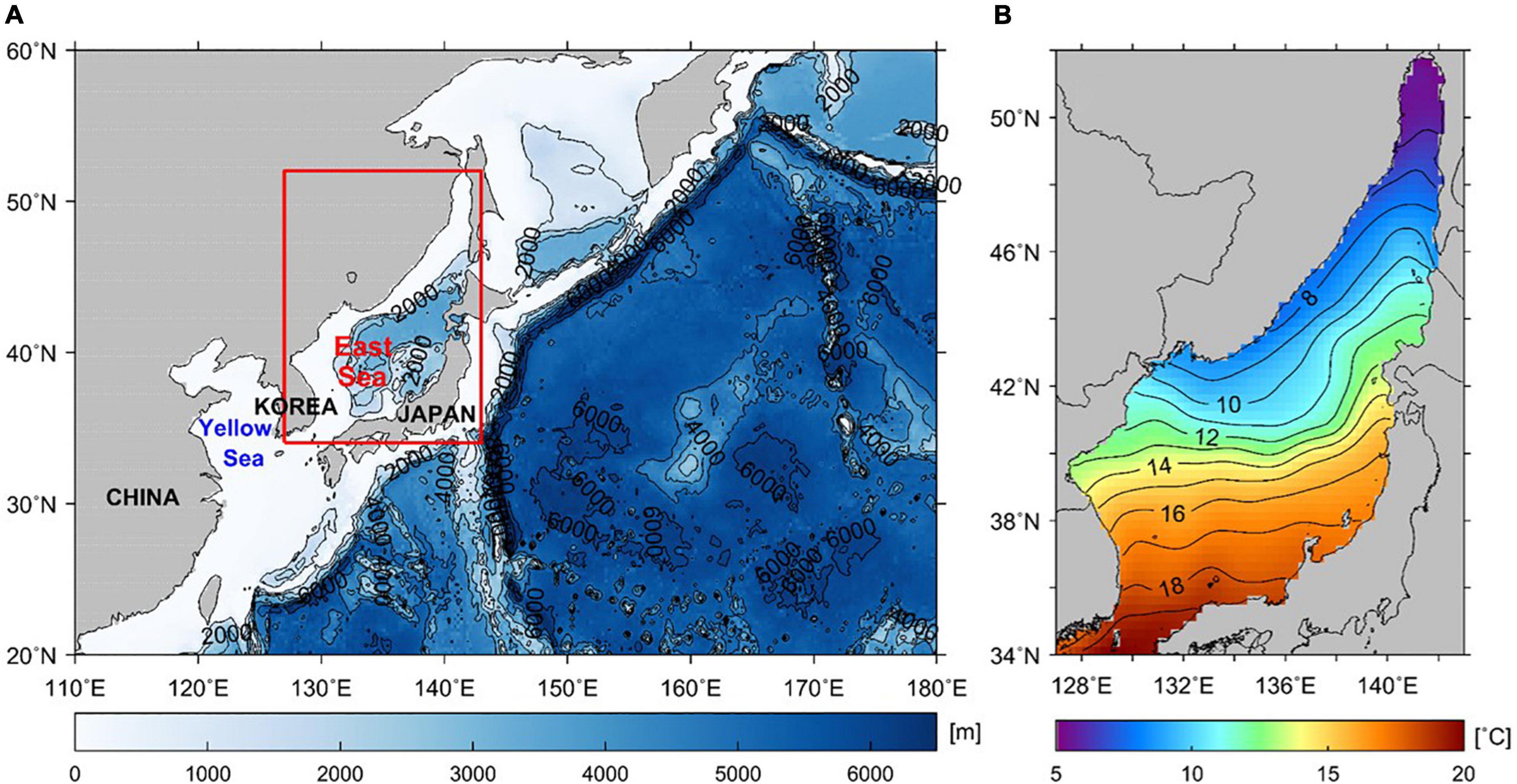
Figure 1. (A) Bathymetry of the Northwestern Pacific, where the red box shows the study area of the East/Japan Sea (EJS), and (B) the spatial distribution of long-term averaged satellite-derived sea surface temperatures (SSTs) for the period from 1982 to 2018.

Therefore, the objectives of this study were to: (1) compute the 100-year-return-period SST value by applying the POT method to the long-term SST observation data in the EJS, (2) compare the results with the maximum SST values observed thus far, and (3) verify the results with those estimated by numerical model simulations based on one of climate change scenarios.

Materials and Methods

Satellite-Observed Sea Surface Temperature Data

The Optimum Interpolation Sea Surface Temperature (OISST) data is one of the most representative SST databases based on Advanced Very High Resolution Radiometer (AVHRR) data with the longest time period from September 1981 to the present. This database was produced by combining observation data from different instruments, including satellites, ships, buoys, and Argo floats. In the process of producing data, objective interpolation was conducted to fill the gaps, and bias adjustment was applied to the observation data to compensate for differences in different observation equipment and sensors (Reynolds and Smith, 1995; Reynolds et al., 2002, 2007; Banzon et al., 2016). The OISST database is a daily product with a spatial resolution of 0.25°. In this study, the OISST version 2 data for the period of from 1982 to 2018 were obtained from the National Oceanic and Atmospheric Administration (NOAA)/Oceanic and Atmospheric Research (OAR)/Earth System Research Laboratory (ESRL) Physical Sciences Lab (PSL)¹ and used to compute the extreme SST value in the EJS.

Simulated Sea Surface Temperature Data of Climate Model

To compare the computed extreme SST values with those predicted from the climate change model, this study used the Coupled Model Intercomparison Project 5 (CMIP5) monthly data on single-level data provided by Copernicus.² The CMIP is a collaborative project designed to improve the existing knowledge about climate change, organized in 1995 by the Working Group on Coupled Modeling (WGCM) of the World Climate Research Program (WCRP) (Meehl et al., 2000). The CMIP data were developed in stages to promote the climate model improvement and support national and international assessments of climate change. The CMIP received model outputs from pre-industrial climate simulations and a 1% annual increase in CO₂ simulations for approximately 30 combined general circulation models. The more recent phases of the project include more realistic climate forcing scenarios for historical, post-phasic, and future scenarios. The main objectives of the CMIP5 experiment are to address the outstanding scientific questions arising from the IPCC Assessment Report (AR) 4, improve understanding of the climate, and provide estimates of future climate change. In this study, the simulation temperature data in the EJS were extracted from global ocean data from December 2005 to November 2099. These data were obtained from the Representative Concentration Pathway (RCP) 4.5 experiment using the HadGEM2-ES model (UK Met Office, United Kingdom).

Extreme Value Analysis for Extreme Sea Surface Temperature

The EVA has been proposed for our study, which is a statistical method that computes extreme values within a certain period of time (e.g., 100 years) from past observation data. It evaluates the probability of events to be more extreme than previously observed (Coles, 2001). Typical EVA methods include the initial distribution method (IDM), block maxima method (BMM), and peaks-over-threshold (POT) method, which are based on the statistical distribution.

First, the IDM is a basic approach for computing extreme values using values from the entire observation data. It approximates that the observation data follow the Gumbel distribution and compute the extreme value corresponding to the probability of the target period (Gumbel, 1958). The total probability density function (PDF) can be estimated using Equation (1), and the probability of the target period is calculated using Equation (2) to find the extreme value by using the time series of SST data at each grid

$F\left(x\right)=exp\left\{-exp\left(\frac{x-\mathrm{\mu }}{\mathrm{\sigma }}\right)\right\}(1)$

$P(x<x_P)=1-\frac{D}{P}(2)$

where σ is the scale parameter, μ is the location parameter, D is the decorrelation time scale, and P is the target period. In this study, 1 year and 100 years were used for D and P, respectively.

Unlike the IDM, which uses the entire observation data, the BMM uses only the maximal values within a block of a specific time period (e.g., a year). These maxima follow a generalized extreme value (GEV) distribution, distribution as shown in Equation (3) (Jenkinson, 1955).

$F\left(x\right)=exp\left[-\left\{1+k{\left(\frac{x-\mathrm{\mu }}{\mathrm{\sigma }}\right)}^{-1/k}\right\}\right](3)$

where k is the shape parameter. The BMM also estimates the value of the probability level corresponding to the target period of the extreme value, as shown in Equation (2). The block units are set to 1 year. That is, the extreme value is computed from the maximum values per year. In this case, the BMM is sometimes referred to as the Annual Maxima Method (AMM).

Finally, in the POT method, it is approximated that values above a certain threshold (e.g., 98th percentile) among all observation data follow the generalized Pareto distribution (GPD) (Coles, 2001). Accordingly, the cumulative PDF is calculated using Equation (4), and the extreme value is computed by calculating the probability level for the target period.

$F\left(x\right)=1-\left\{1+k{\left(\frac{x-\mathrm{\mu }}{\mathrm{\sigma }}\right)}^{-1/k}\right\}(4)$

$P(x<x_P)=1-\frac{N_Y}{P{N}_{POT}}(5)$

where μ is the threshold parameter. N_Y is the number of years of data and N_POT is the total number of data used in the POT analysis. In recent studies, the POT method has been widely applied to compute the extreme value, namely, the long-period return value (e.g., Caires and Sterl, 2005; Laurent and Parey, 2007; Cheng and AghaKouchak, 2014).

The confidence intervals were calculated with the computed extreme SSTs. According to Coles (2001), the variance of the long-period return value is calculated using the variance-covariance matrix and the delta method as follows:

$Var\left(x_P\right)\approx {\left(\nabla x_P\right)}^{T}V\left(\nabla x_P\right).(6)$

In Equation (6), the complete variance-covariance matrix V for (ζ_μ,σ,k) is

$V=\left[\begin{array}{ccc}\hfill {\mathrm{\zeta }}_{\mu }(1-{\mathrm{\zeta }}_{\mu })\hfill & \hfill 0\hfill & \hfill 0\hfill \\ \hfill 0\hfill & \hfill v_{1,1}\hfill & \hfill v_{1,2}\hfill \\ \hfill 0\hfill & \hfill v_{2,1}\hfill & \hfill v_{2,2}\hfill \end{array}\right](7)$

where ζ_μ is the proportion of data exceeding μ and v_i,j is the variance-covariance matrix of σ and k. (∇⁡x_P)^T is calculated using Equation (8).

${\left(\nabla x_P\right)}^T=\left[\begin{array}{ccc}\hfill \frac{\partial x^T}{\partial {\mathrm{\zeta }}_{\mathrm{\mu }}}\hfill & \hfill \frac{\partial x^T}{\partial \mathrm{\sigma }}\hfill & \hfill \frac{\partial x^T}{\partial k}\hfill \end{array}\right](8)$

In this study, we mainly used the POT method to compute extreme SST values using satellite data. Although the POT method complements the defects of the prior method, the variations in its calculated extreme value were amplified if the data for this approach were insufficient (see section “Discussion”). Because the estimated values of the parameters vary depending on the threshold value, it is necessary to consider which value to be selected as the threshold (e.g., 98th percentile). The details of the method applied in this study are explained in the following section.

Statistical Methods for Extreme Sea Surface Temperature Computation

Figure 2 shows the example results of computing extreme SSTs by applying the three representative EVA methods to the long-term satellite SST observation data at an arbitrary point (133.88° E, 37.88° N) in the central region of the EJS. Figures 2A,B show the approximation results by applying the IDM to all of the daily data and the BMM to the annual maximum daily data from 1982 to 2018, respectively. Figure 2C shows the result of applying the POT method to satellite SST values, which is approximated by assuming that the values above the threshold (98th percentile in this study) follow the GPD. Consequently, the 100-year-return-period SST was computed as 29.55, 30.13, and 29.74°C by the IDM, BMM, and POT methods, respectively. All the computed extreme SSTs were higher than the mean values of the upper 5th-percentile SSTs of 26.62°C.

FIGURE 2

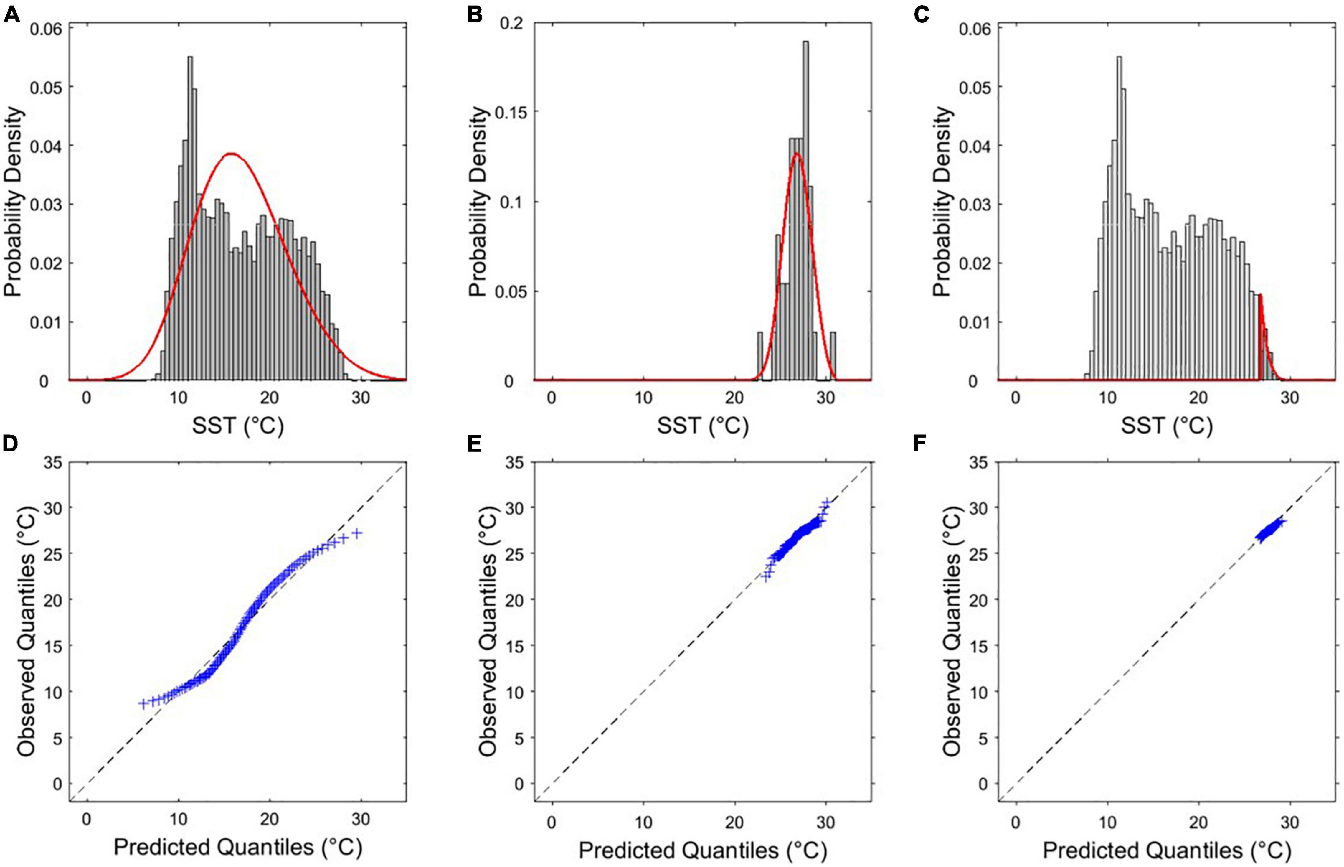
Figure 2. Examples of the distribution of probability of SST values, where the red line represents the fitted distribution for the computation of the extreme SST by (A) initial distribution method (IDM), (B) block maxima method (BMM), and (C) peaks-over-threshold (POT) method, respectively. (D–F) The comparison results between the predicted and observed quantiles from panels (A–C).

The approximation accuracy of each statistical distribution varies depending on the characteristics of the SST distribution at each point. Overall, as shown in the quantile-quantile plot (Q-Q plot) in Figure 2D, the SST does not exactly follow the Gumbel distribution of the IDM. Although the GEV distribution of BMM seems to be comparatively well-followed, few differences still exist between the points. This may be a limitation owing to the use of only the annual maximum value among the data (Figure 2E). In contrast to the IDM and BMM, the POT method, applied to the long-term return SST values, produced the most appropriate coincidences between the predicted and observed quantiles with remarkable fitting to the GPD with values over a specific threshold (e.g., 98th percentile; Figure 2F). The predicted quantiles using the probability density fitted by POT show good agreement with the observed quantiles from the satellite data; therefore, we computed the 100-year SST values by applying the POT method in this study.

The detailed process of the POT method is shown in Figure 3. First, after loading the daily SST data, the values out of three standard deviations within a 3 × 3 (∼ 0.75° × 0.75°) window were removed to remove abnormally high or low SST values. If there is a trend in the observed data over time, a non-stationary model is applied because the assumption of stationarity cannot be applied (Coles, 2001; Khaliq et al., 2006). In the global ocean, previous studies have revealed an obvious warming trend (Baker et al., 2004; Sutton et al., 2007; IPCC Climate Change, 2014; Stott, 2016). Similarly, the warming trend of the EJS has been well-documented in numerous studies (e.g., Kim et al., 2001; Yeh et al., 2010; Lee and Park, 2019). Prior to the computation of the extreme value based on the GPD fitting, the stationarity or non-stationarity of the SST data was determined through the Mann-Kendall test with the SST anomaly time series in which the annual cycle was removed (Mann, 1945; Kendall, 1955). The analysis showed that the SST data of the EJS could be regarded as non-stationarity, indicating a significant warming trend mainly caused by the mean trend except for a few points. Therefore, the coefficients were estimated by reflecting the non-stationary characteristics in the subsequent fitting process. In this study, the scale parameter was given as a parameter that changes with time, and a linear model was applied as follows:

$\mathrm{\sigma }\left(\text{t}\right)={\mathrm{\sigma }}_0+{\mathrm{\sigma }}_1\text{t}(9)$

FIGURE 3

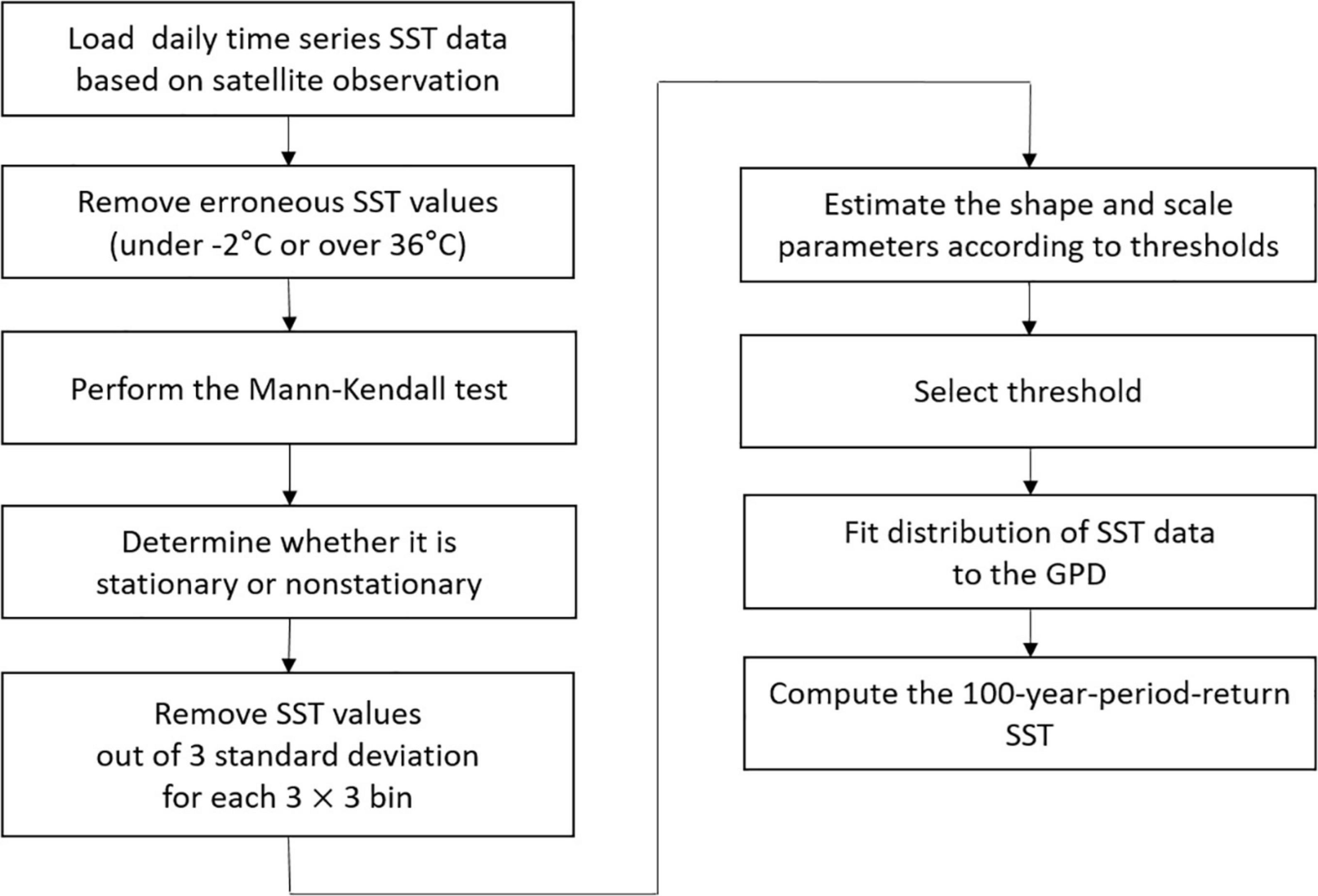
Figure 3. Flow chart for the computation of extreme SST using the POT method based on generalized Pareto distribution (GPD).

for parameters σ₀ and σ₁. The maximum likelihood estimation was applied to estimate the parameters of the GPD (Fisher, 1925). The application of this non-stationary model with a linear trend in the scale parameter was confirmed using the likelihood ratio test (Koch, 1988). The long-period return level computed by applying the non-stationary model changes with time, as more observed data were added from the past to the latest. The longer the return period, the more the deviation between extremes from non-stationary and stationary models tends to increase.

Another important process is setting the thresholds for POT. In this study, the 98th-percentile value was selected as the threshold by checking the change and significant interval of the shape (k) and scale (σ) parameters according to the threshold setting, as shown in Figure 4. We selected the thresholds marked by red dots in Figure 4. These values have also been used in previous studies (Laurent and Parey, 2007; Parey et al., 2007; Cheng et al., 2014), which compute the extreme values of surface air temperatures. A similar approach was applied to calculate the extreme values of precipitation (Cheng and AghaKouchak, 2014).

FIGURE 4

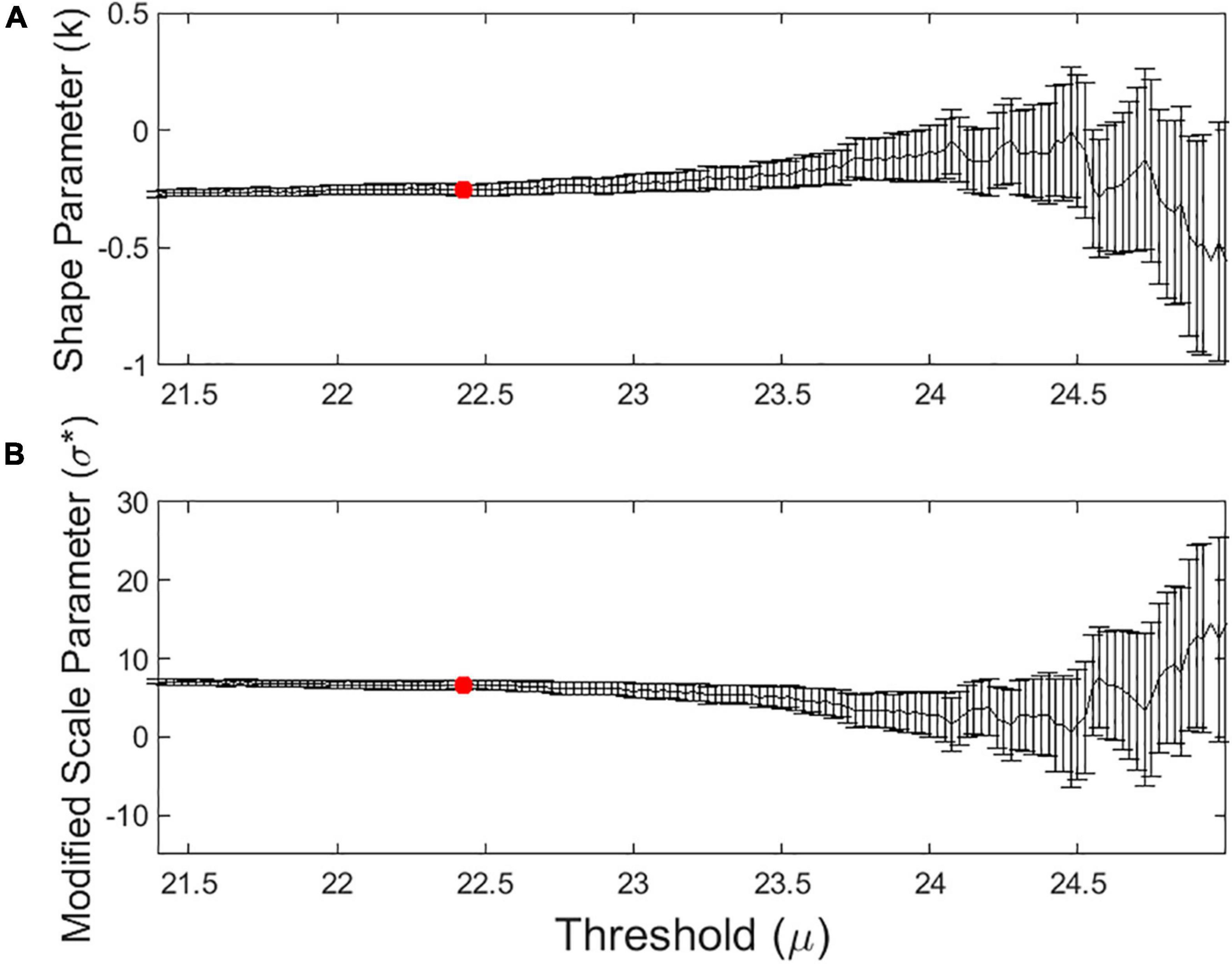
Figure 4. (A) Shape parameter (k) and (B) modified scale parameter (σ*) with 95% confidence intervals for every value of the threshold (μ). The red dot indicates the 98th percentile of SSTs.

Results

An Example of the Computation of Extreme Sea Surface Temperature

Prior to applying the POT analysis to the entire EJS region, we tested whether this method could successfully resolve the 100-year-return SST value as an extreme value at an arbitrary position. The position was selected in the central region (133.88° N, 37.88° E), and a time-series of daily SSTs was extracted for the study period. The time-variable SST data of the EJS has an obvious tendency to increase with time, with statistical significance. Based on this test, we assumed that the SST data could be treated as non-stationary data; under this assumption, a non-stationary POT analysis method is applied. The expected return level of SST for each return period was calculated using the 95th-percentile confidence interval. The confidence interval was calculated using the method described by Coles (2001).

Figure 5 shows the results of the long-period-return level of SST values as a function of return periods up to 100 years, calculated by applying the POT method using the long-term satellite SST observation data at the point. The dashed lines in Figure 5 represent the upper and lower limits of the return SST levels for each given return period from 1 to 100 years. The differences between the upper and lower levels within the 95% confidence intervals were amplified with increasing return periods. As the return period increased from 1 to 100 years, the return level of SST tended to rapidly increase at a range of relatively small return periods of <20 years and gradually increased from 60 to 80 years, and eventually converged toward a 100-year return SST with feeble increasing features. The computed extreme SST value, corresponding to a 100-year return value, was approximately 28.93°C as shown by the solid line at a return period of 100 years. Within the 95% confidence level, the lower and upper extreme values were 28.77 and 29.11°C, with a difference of 0.34°C. This feature suggests that the present approach of POT analysis can yield a computation of extreme SST values.

FIGURE 5

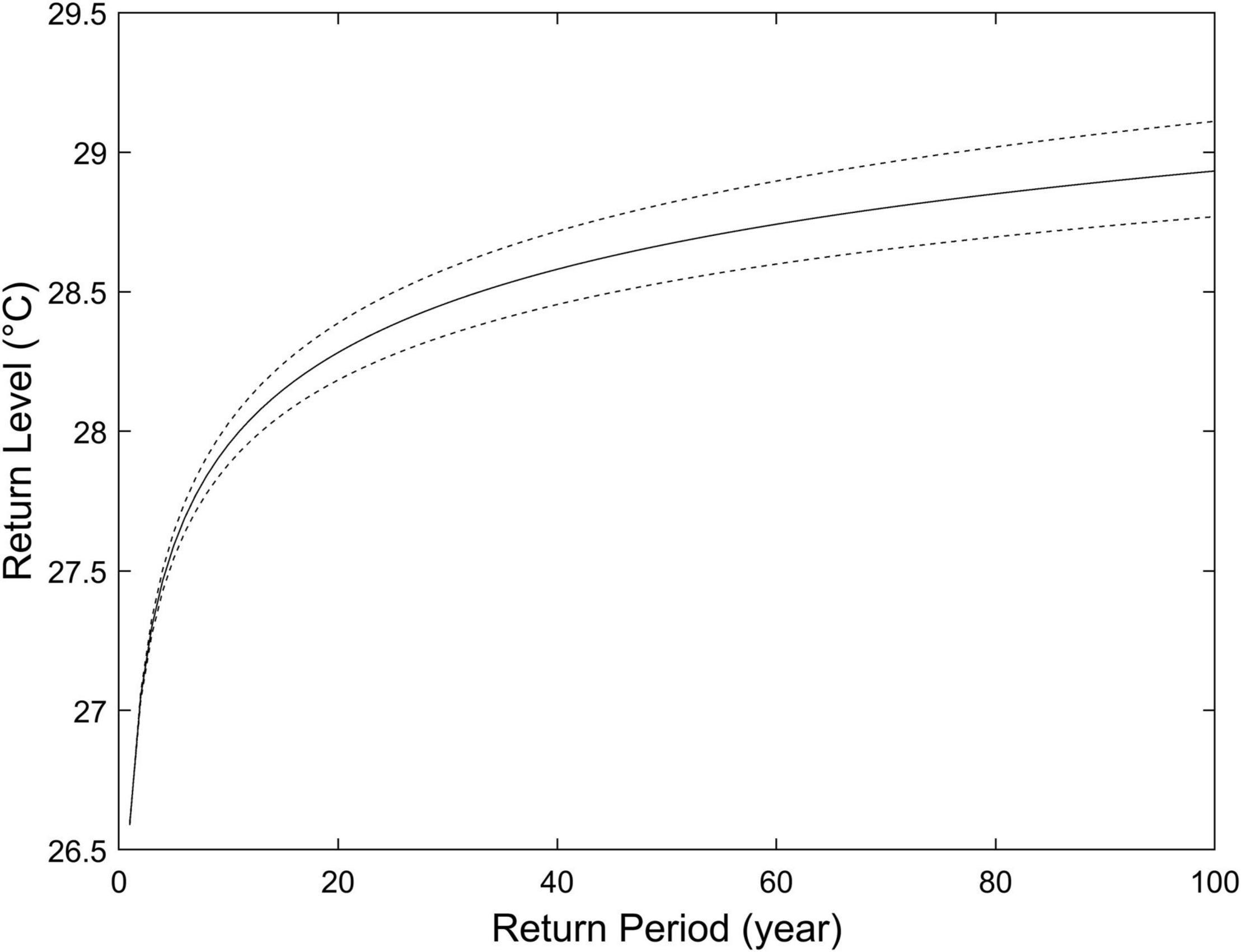
Figure 5. An example of the result of extreme SST derivation (solid line) using the POT method under the assumption of non-stationary data, wherein the dashed lines represent the limits of the 95% confidence interval.

Spatial Distribution of Extreme Sea Surface Temperatures

To calculate the 100-year SST in the entire area of the EJS by applying the POT method, the parameters were first estimated using the maximum likelihood estimation method. Figure 6 shows the estimated parameters for the optimal fitting of the SST data above the threshold to the GPD at each point. As shown in Figure 6, the threshold (μ) showed a similar distribution to that of the mean SST value at each point, and the shape parameter (k) and scale parameter (σ₀) also seemed to indicate the SST distribution characteristics according to the points. Overall, a spatial regularity was confirmed. We computed the 100-year SSTs by applying the POT method to the satellite-observed SST dataset for the entire area of the EJS (Figure 7A). The spatial distribution of the computed 100-year SST was similar to that of the mean SSTs in the EJS with contrasting north-south temperatures across the subpolar front, roughly along 40° N in the central part (Park et al., 2007). The isotherms of the computed 100-year SSTs ranged from a minimum value of 19.04°C in the northern part to a maximum value of 30.96°C in the southern part of the EJS. Overall, the computation of 100-year-return SSTs showed values higher than approximately 26°C south of the subpolar front along 40° N. In particular, along the western coast of Japan, the extreme SST reached approximately 28°C around the Tsugaru Strait near 41° N and approximately 24°C around the Soya Strait near 45° N. These extreme values are considerably higher than those in the western part of the EJS. This implies that the spatial distribution of extreme SSTs was similar to the pattern of mean SSTs with higher SSTs due to the Tsushima Warm Current along the western coast of Japan.

FIGURE 6

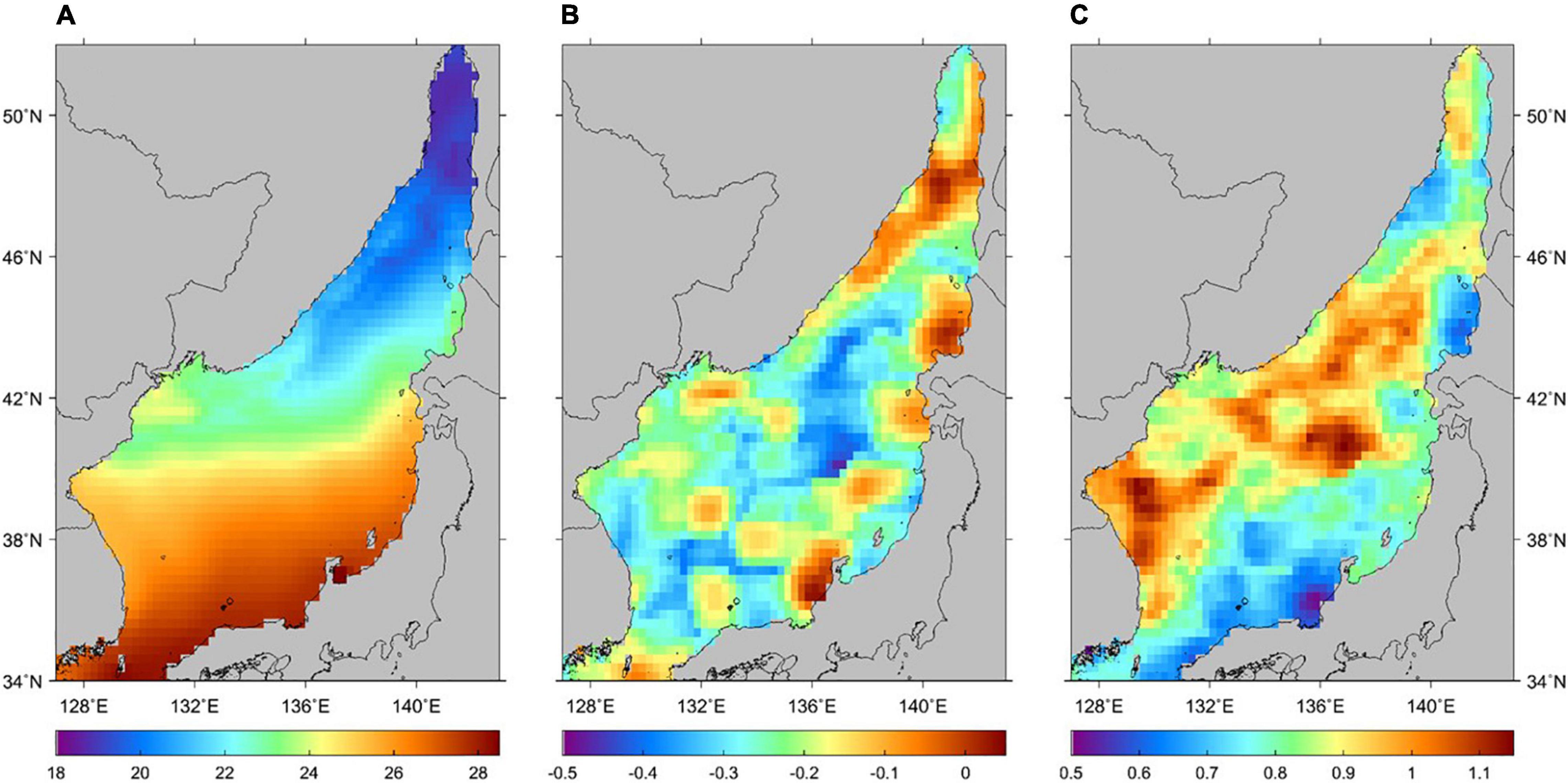
Figure 6. Spatial distribution of estimated parameters for GPD. (A) threshold (μ), (B) shape parameter (k), and (C) scale parameter (σ₀).

FIGURE 7

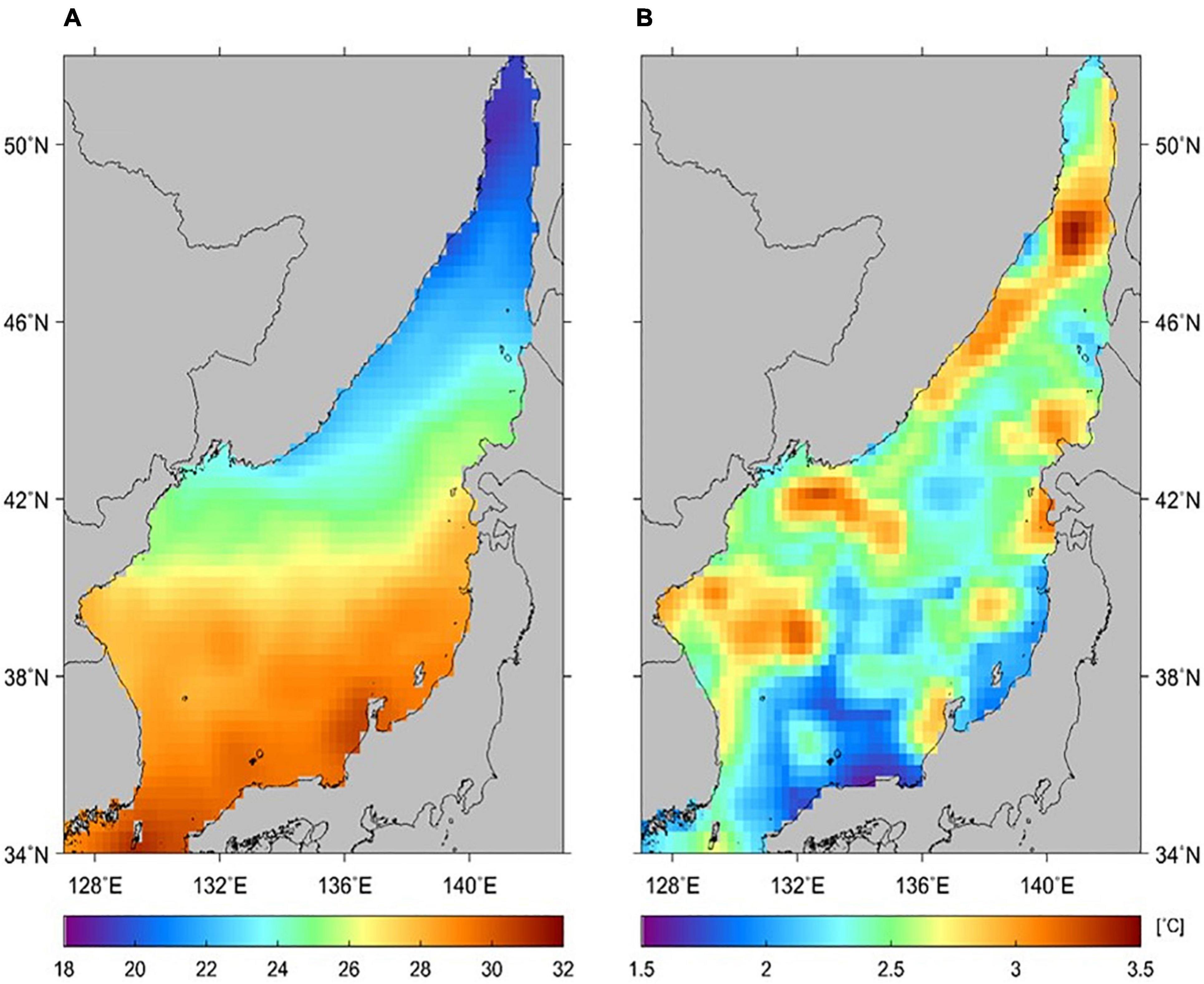
Figure 7. (A) Computed result of the 100-year SST using the POT method and (B) difference between the computed result of the 100-year SST and mean of the upper 5th percentile of observed SST (100-year SST minus the maximum SST) using satellite SST data from 1982 to 2018.

To understand how large such 100-year-return extreme SST values are compared to the maximum records of SST values over the past decades, we derived the maximum SSTs by considering the average of the upper 5th-percentile SST values observed in the past 37 years (1982–2018). Figure 7B shows the SST differences between the 100-year SST and the mean value of the upper 5th-percentile of the observed SST. Overall, the differences ranged from 1.60 to 3.44°C, which implies that the calculated 100-year SST value was higher than the mean of the upper 5th-percentile SST in the past in the entire EJS. In other words, it signifies that considerably higher extreme SST would occur in the future compared to the past extreme SST in all areas of the EJS. The maximum difference between the extreme SST in the future and that in the past amounted to 3.44°C in the northern part. The northwestern part, including the offshore regions off the Russian coast, south of Vladivostok, and over West Korea Bay, showed relatively high values of 2.70°C. This region coincides with that affected by strong winds from the continental side during winter. In contrast, the southern region showed relatively low differences in the extreme SST. One important feature is that all the 100-year return SST values are positive in the entire EJS. This suggests that the warming features of extreme SSTs will be strengthened in the future.

Monthly Distribution of Extreme Sea Surface Temperatures

The SSTs of the EJS have dominant seasonality with higher amplitudes of approximately 9°C at most than those of the Northwest Pacific at similar latitudes (Park et al., 2005). Thus, it is necessary to understand the seasonal distinctions of extreme SST values in space. Prior to the derivation of the seasonal variations, it was necessary to check whether the computed extremes were statistically significant by applying the POT method to the monthly observation data. GPD fitting was conducted on the observed data distribution at a point (134.88° E, 42.88° N) for each month from January to December (Figures 8A–L). In each monthly plot, the red curves represent the fitted GPD distributions at relatively high SSTs during each month. As inferred from the tail of the GPD distribution, the end of the tail reached a much higher temperature range by revealing a slower decrease in August compared to January, with a rapid drop in the GPD distribution. Therefore, it is expected that the extreme SSTs would yield much higher values in summer than in winter, with exceptions near the frontal region. As a result of the Q-Q plots of all months in Figure 8M, we found that all the monthly data distributions followed the GPD well for all months. The predicted quantiles showed good agreement with the observed quantiles of the SST data for each month from January to December. This coincidence implies that monthly SST data are statistically significant enough to calculate monthly 100-year SSTs.

FIGURE 8

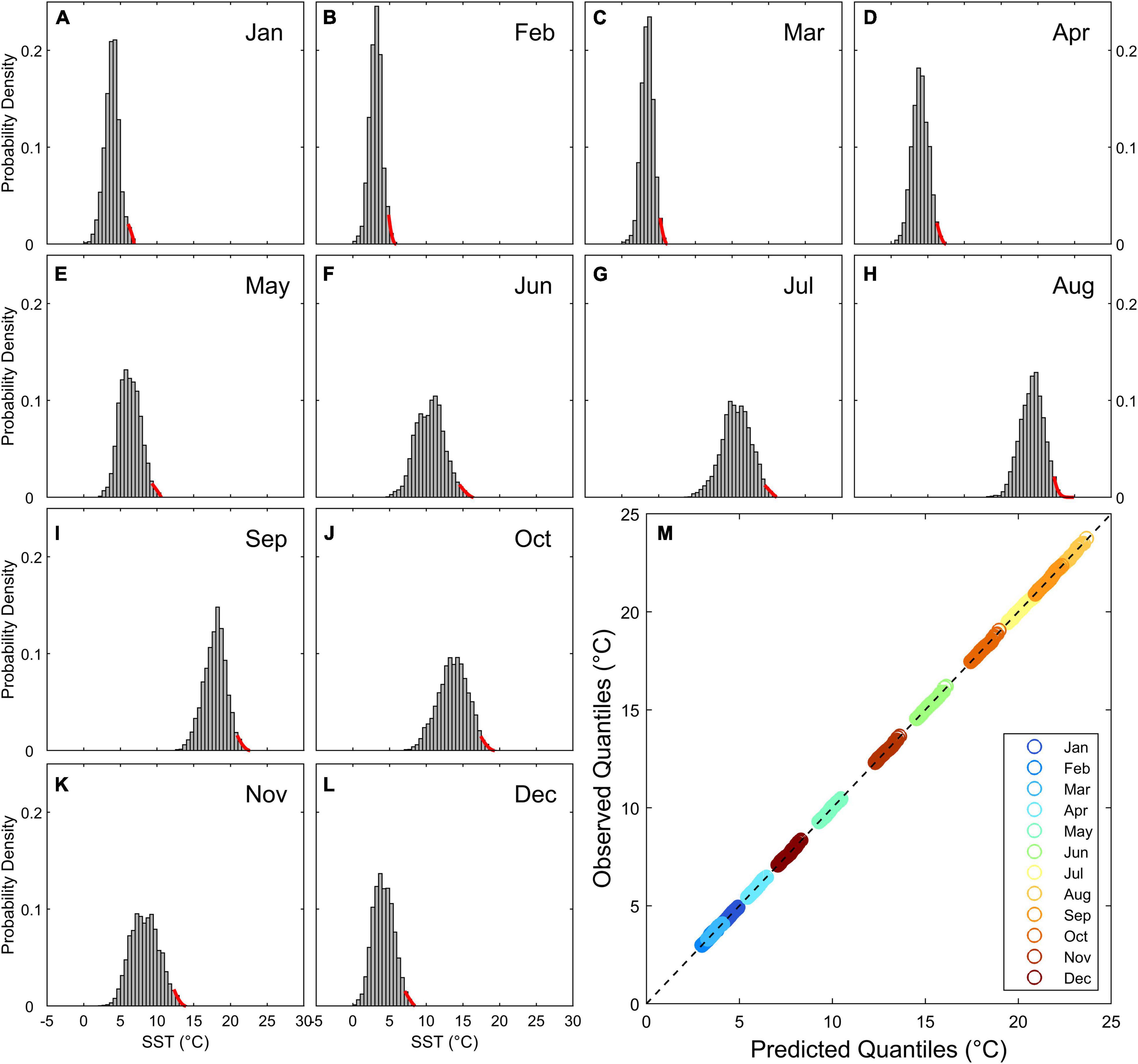
Figure 8. Examples for the computed result of the monthly extreme SST. (A–L) Distribution of the probability of monthly SST values, where the red line represents the fitted distribution for the computation of the extreme SST by the POT method and (M) Q-Q plot for all months.

Based on the aforementioned results, monthly 100-year return extreme SSTs of the entire EJS were calculated using the POT method. As shown in Figure 9A, the extreme SST was highest in August and lowest in February, similar to the seasonal variational characteristics of the SST in the EJS. The monthly distribution of SST extremes showed the general features of SST distribution. However, highly extreme SSTs up to 40°C were derived at some points with a red circle-like feature in the southern part of the EJS in August. This may be induced by the POT method, which computes the extreme values based on the statistical distribution function by analyzing only past observations. Overall, potential extreme values were simulated comparatively well by the POT method. However, if the number of observed data is insufficient, the method may have limitations in computing abnormally large values, as mentioned in the previous section (Materials and Methods); this is further discussed in the subsequent section (“Discussion”). Figure 9B shows the monthly maps of the differences between the computed 100-year SST values and the mean of the upper 5th-percentile SST values over the past decades. Regardless of time, all monthly difference maps illustrated positive differences larger than 0.18°C, implying that extreme SST estimations appeared larger than the past observations over the entire EJS. The computed extremes exceeding 2°C were distributed near the subpolar front in the central region from December to April, in contrast with relatively low differences in the northern and southern regions, which were <1°C. The smallest differences appeared with an average of 0.95°C in March. In contrast, the positive differences were broadly distributed over the entire region of the EJS, with particular amplified features in October and November. The derived SST extremes tended to be much higher than the observed maximum SSTs in summer (June to August) and autumn (October and November).

FIGURE 9

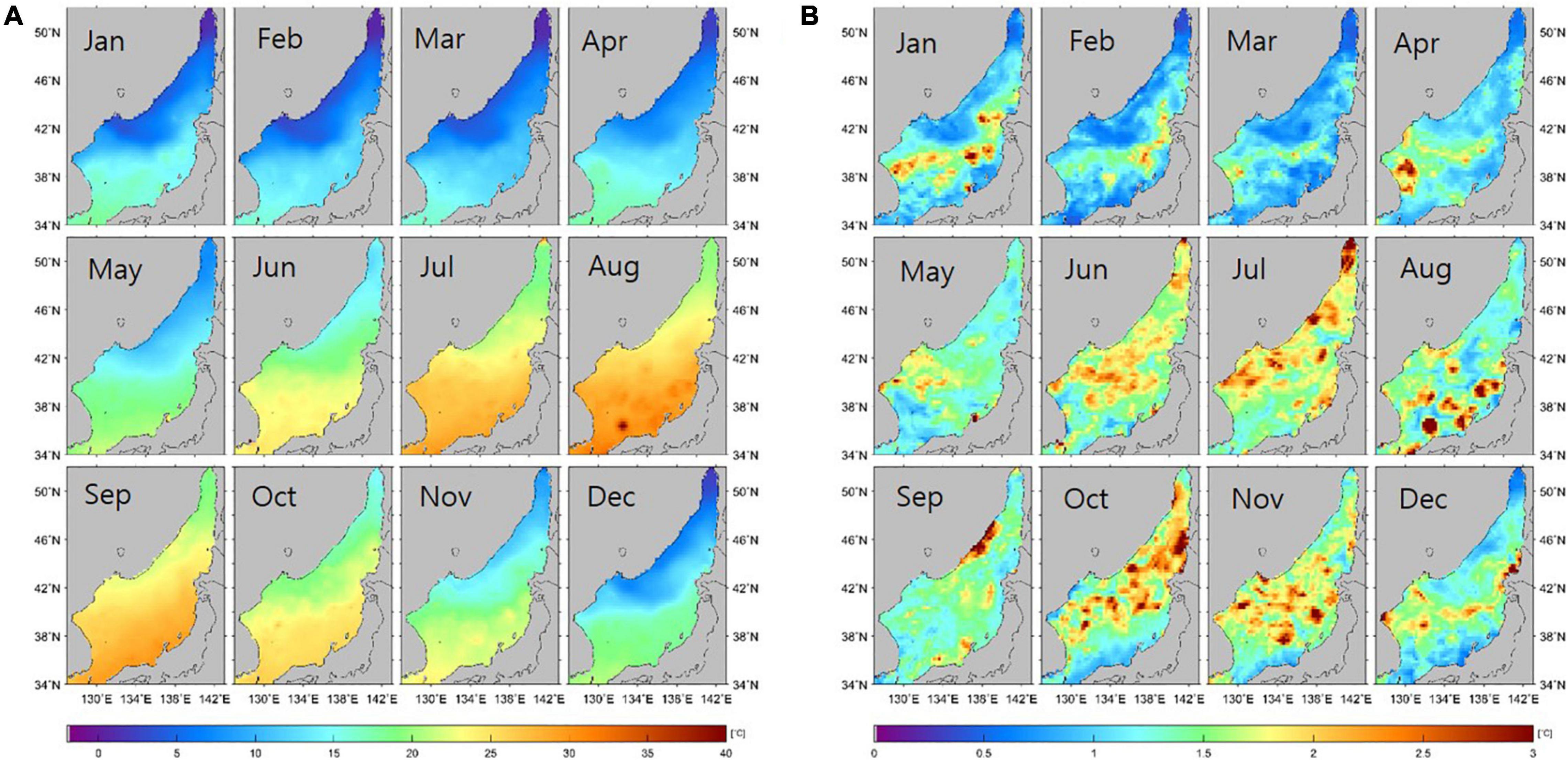
Figure 9. Spatial distribution of (A) monthly 100-year return SSTs using the POT method and (B) temperature differences between the computed SST extremes and mean values of satellite-observed SSTs (1982–2018) within the upper 5th percentile.

In order to analyze the monthly variations of the difference in Figure 9B more quantitatively, the number of pixels with differences >2°C for each month is plotted in Figure 10. The number histogram showed that the relatively higher extremes, as compared with the upper 5th percentile of the SST data, showed high values in the order of October, July, November, and June. In contrast, small extremes appeared in March and February. Overall, there are many pixels where the extreme SST is computed to increase significantly from June to November. That is, it was expected that the 100-year return SSTs would be much higher (>2°C), mainly in the summer–autumn period. Conversely, in late winter–early spring (February–March), the 100-year SST was computed to be not considerably higher than in the past (<2°C) at many points. This seasonal distribution is similar to that of the warming trends in the EJS, as presented in a previous study (Lee and Park, 2019).

FIGURE 10

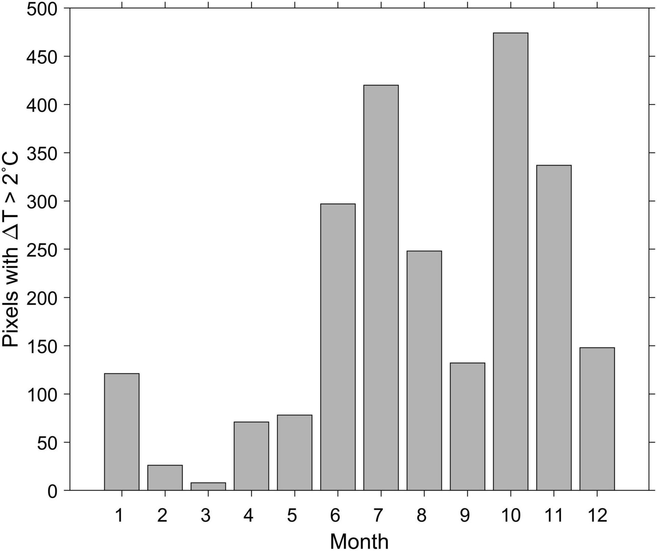
Figure 10. The number of pixels with differences over 2°C between the computed 100-year SSTs and mean satellite-observed SSTs within the upper 5th percentile from 1982 to 2018.

Comparison of the Computed Extreme Sea Surface Temperatures to Numerical Model Simulation

The results of numerical simulations have been extensively used to understand SST warming in the future. CMIP5 is one of the representative models for climate change scenarios. Using the model results of the selected CMIP5 model, we obtained the monthly mean SST value for the period from 2005 to 2099, which is closest to the 100-year future. Figure 11 shows the spatial distribution of the maximum SST values for each pixel for the future period. Although the spatial grid is too large to represent the spatial distinction, there is an obvious contrast in temperatures between the northern and southern parts. The simulated maximum values ranged from 16.52°C in the northern part to 33.14°C in the southern part. One remarkable feature was found in the near-coast regions of Japan (34°–40° N) and North Korea (∼40° N). The simulated temperatures were distributed in a wider range compared to the 100-year SST value (19.04–30.96°C) computed by applying the POT method to the OISST data for the past 37 years (Figure 7A). There were slight differences between the computed SST extremes and the simulated model SSTs in terms of the temperature and spatial distribution. The model SST maximum revealed a characteristic feature with higher SSTs in the coastal region of the Korean Peninsula and Japanese coast than those in the open sea areas. Concentrated on the isotherm of approximately 26°C, the maximum SSTs from the model simulation were spatially dominant in the coastal region of the Korean Peninsula up to 42 °N compared to the offshore region in the central part of the EJS. The limitation of this characteristic distribution is that it is difficult to compare accurately because both satellite and model data have relatively low accuracies in coastal regions (Lee and Park, 2020). In particular, for different spatial resolutions, 1° resolution model data and 0.25° resolution satellite data produced relatively large errors in the coastal region.

FIGURE 11

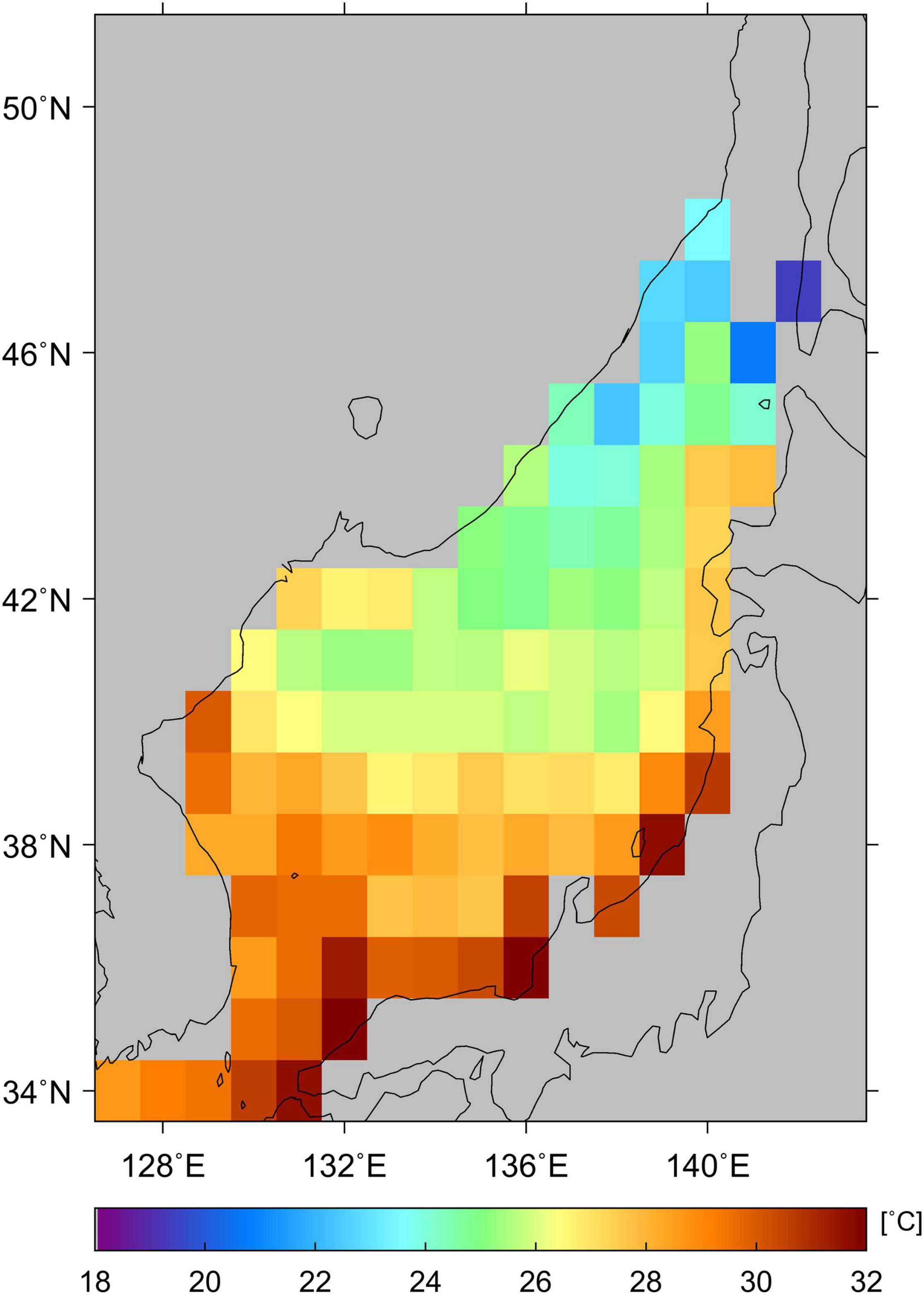
Figure 11. Spatial distribution of CMIP5 model-simulated maximum SSTs for a period from December 2005 to November 2099 in the future.

Figure 12 shows a comparison between the computed 100-year SST values and simulated SST values from the CMIP5 model. The computed 100-year SST values included in the CMIP5 model grid with a 1° interval were averaged and compared with the model-estimated maximum value. In narrow channels such as the Tatar Strait in the northern EJS, the comparison is impossible owing to large differences in the grids. Accordingly, the data in the northern part at latitudes higher than 46 °N were excluded from the comparison because of their low spatial resolutions. The maximum value of the model-simulated SST data ranged from 22.36 to 33.14°C, and the 100-year SSTs calculated from the OISST data ranged from 21.98 to 30.62°C. The differences between the two values (computed 100-year SST–model-simulated maximum SST) were close to zero when the model-simulated maximum SST was in the middle range of 25–28°C. However, in other ranges, the 100-year SST values tended to be lower than the model results. The bias of the differences was negative at about –0.36°C, implying higher SST maximum values than the 100-year SST computations. The RMS of the differences amounted to 1.33°C. As both SST extremes are fundamentally different in terms of the conceptual approach, the relatively high RMS and bias errors do not emphasize which SSTs are more pertinent to understanding the extreme SST values. Additionally, both data have uncertainties, such that the brief coincidence of the trends can be acceptable for understanding the upcoming SST extremes in the future.

FIGURE 12

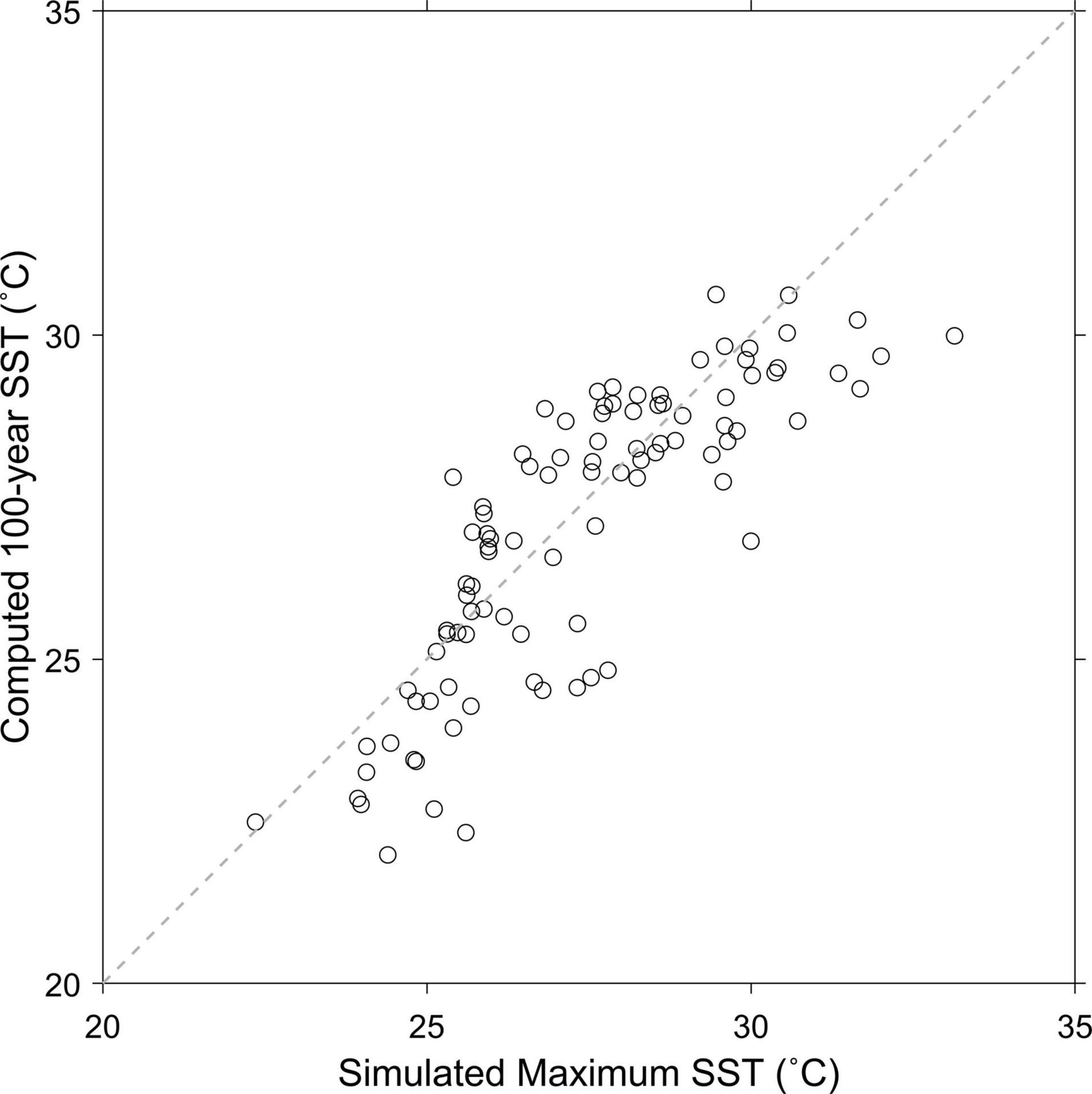
Figure 12. Comparison of the computed 100-year return SSTs based on the POT method and the maximum SSTs from the CMIP5 model-simulated data for a period from December 2005 to November 2099.

Discussion

Abnormally High Sea Surface Temperature Extremes

In this study, we have shown the possibility that extreme SSTs could be computed as long-period-return SSTs by applying the POT method through satellite-observed data. However, some pixels produced abnormally high extreme SSTs of >40°C in the application of monthly extremes, especially in August, with an annual maximum for a year (Figure 9A). Unexpected high extremes of this type can be produced in the following cases: the first case can be found when high SST values are rarely observed because of the low observation frequency of large values. Relatively small data facilitate the generation of an unusually long tail in the direction of the higher SST values in the GPD fitting process. This tendency may produce the computed extreme SSTs from the fitted PDF curve. This problem originating from the low number of observations is expected to be resolved as more data are collected with the extension of the observation period. Extremely high SSTs with spatial dominance were detected in only a few pixels in a certain month of summer. From this perspective, the computed SST extremes over the entire period can be regarded as reasonable results fitted comparatively well to the GPD.

Uncertainty of the Result From the Model Simulation

For the comparison of the 100-year return extreme SSTs based on the POT method, this study selected one of the prediction results of the climate change models. As the result of the comparison, the two SST extreme values showed a similarity in the overall spatial distribution, except for some coastal areas. There were slight differences with a bias of –0.36°C and an RMS difference of 1.33°C. These differences can be regarded as acceptable errors because of substantial differences in the present approach from the maximum SSTs of the climate model simulation. Additionally, both the 100-year SST extremes and the model prediction results have their own uncertainty from different sources. Model simulation requires several assumptions with many limitations and arguments. The present approach focuses only on the statistical shape of the non-stationary data. In terms of dealing with extreme values, however, the model results were positively comparable to the results of this study with similar spatial patterns. It is encouraging that the POT method can be applied to satellite SSTs and can simulate a similar feature to the climate model without the limitation of computations for a complete understanding of the climate system. In light of this, our study can help us know in advance what the future oceanic world will look like though rough statistical predictions of extreme SSTs in the future based on satellite-observed SST data over the past decades.

Conclusion

In this study, we computed the 100-year return SSTs, as extreme SSTs, using the POT method as a statistical method for non-stationary data. Prior to the application of the non-stationary method, we investigated whether the satellite SST data can be treated as non-stationary data through significance tests of the long-term trend of the SSTs within the 95-percent confidence level. The POT method was superior to other methods (IDM and BMM) in deriving extreme SSTs based on the GPD statistical distribution. The POT application confirmed the possibility of computing extreme SSTs. The results presented that extreme SSTs were higher than the maximum SSTs of previously observed satellite data by 1.60–3.44°C. Monthly variations of the SST extremes revealed proper features except for a few pixels, partly because of less observation in the local regions in summer. The spatial distribution of the computed SST extreme values showed good agreement with the maximum SSTs predicted by the model simulation of climate change. The magnitudes of the extreme SSTs were comparable to the model-simulated SSTs.

Based on these results, the EVA method, especially the POT method, can be useful tools to compute the long-term return SSTs as an alternative to model prediction, which requires a large amount of input data and a long computational execution time. This study was the first to use the POT method to derive the 100-year return extreme values of SST as one of the most representative oceanic and atmospheric variables, and suggested the possibility of its application in understanding the future ocean using satellite SST data accumulated over the past decades. This study focused on the EJS; however, it can be extended to the global ocean as well as to many marginal seas. Thus, this study is expected to contribute to the monitoring of future extreme SST changes in the global ocean.

Data Availability Statement

The original contributions presented in the study are included in the article/supplementary material, further inquiries can be directed to the corresponding author.

Author Contributions

K-AP conceptualized and organized the study and rewrote and edited the whole text. E-YL collected and processed the datasets used in the manuscript, further-developed the algorithms, prepared all figures and tables, and wrote the first version of the manuscript. Both authors contributed to the final version of the manuscript.

Funding

This study was supported by the National Research Foundation of Korea (NRF), grant funded by the Korean Government (MSIT) (No. 2020R1A2C2009464). Data processing was partly supported by the project entitled “Deep Water Circulation and Material Cycling in the East Sea (20160040),” funded by the Ministry of Oceans and Fisheries, South Korea.

Conflict of Interest

The authors declare that the research was conducted in the absence of any commercial or financial relationships that could be construed as a potential conflict of interest.

Publisher’s Note

All claims expressed in this article are solely those of the authors and do not necessarily represent those of their affiliated organizations, or those of the publisher, the editors and the reviewers. Any product that may be evaluated in this article, or claim that may be made by its manufacturer, is not guaranteed or endorsed by the publisher.

Acknowledgments

NOAA High Resolution SST data provided by the NOAA/OAR/ESRL PSL, Boulder, CO, United States, from their Web site at https://psl.noaa.gov. We acknowledge the World Climate Research Programme’s Working Group on Coupled Modeling, which is responsible for CMIP, and we thank the climate modeling groups for producing and making available their model output. For CMIP the US Department of Energy’s Program for Climate Model Diagnosis and Intercomparison provides coordinating support and led development of software infrastructure in partnership with the Global Organization for Earth System Science Portals.

Footnotes

1. ^ https://psl.noaa.gov
2. ^ https://cds.climate.copernicus.eu

References

Baker, A. C., Starger, C. J., McClanahan, T. R., and Glynn, P. W. (2004). Corals’ adaptive response to climate change. Nature 430:741. doi: 10.1038/430741a

PubMed Abstract | CrossRef Full Text | Google Scholar

Banzon, V., Smith, T. M., Chin, T. M., Liu, C., and Hankins, W. (2016). A long-term record of blended satellite and in situ sea-surface temperature for climate monitoring, modeling and environmental studies. Earth Syst. Sci. Data 8, 165–176. doi: 10.5194/essd-8-165-2016

CrossRef Full Text | Google Scholar

Caires, S., and Sterl, A. (2005). 100-year return value estimates for ocean wind speed and significant wave height from the ERA-40 data. J. Clim. 18, 1032–1048. doi: 10.1175/JCLI-3312.1

CrossRef Full Text | Google Scholar

Cheng, L., AghaKouchak, A., Gilleland, E., and Katz, R. W. (2014). Non-stationary extreme value analysis in a changing climate. Clim. Change 127, 353–369. doi: 10.1007/s10584-014-1254-5

CrossRef Full Text | Google Scholar

Cheng, L., and AghaKouchak, A. (2014). Nonstationary precipitation intensity-duration-frequency curves for infrastructure design in a changing climate. Sci. Rep. 4:7093. doi: 10.1038/srep07093

PubMed Abstract | CrossRef Full Text | Google Scholar

Coelho, C. A. S., Ferro, C. A. T., Stephenson, D. B., and Steinskog, D. J. (2008). Methods for exploring spatial and temporal variability of extreme events in climate data. J. Clim. 21, 2072–2092. doi: 10.1175/2007jcli1781.1

CrossRef Full Text | Google Scholar

Coles, S. (2001). An Introduction to Statistical Modeling of Extreme Values. London: Springer.

Google Scholar

Fisher, R. A. (1925). Theory of Statistical Estimation. In Mathematical Proceedings of the Cambridge Philosophical Society. Cambridge: Cambridge University Press.

Google Scholar

Gumbel, E. J. (1958). Statistics of Extremes. New York, NY: Columbia University Press.

Google Scholar

Huser, R. (2021). EVA 2019 data competition on spatio-temporal prediction of Red Sea surface temperature extremes. Extremes 24, 91–104. doi: 10.1007/s10687-019-00369-9

CrossRef Full Text | Google Scholar

Ichiye, T. (1984). “Some problems of circulation and hydrography of the Japan Sea and the Tsushima current,” in Ocean Hydrodynamics of the Japan and East China Seas, Elsevier Oceanogr. Ser, Vol. 39, ed. T. Ichiye (New York, NY: Elsevier), 15–54. doi: 10.1016/s0422-9894(08)70289-7

CrossRef Full Text | Google Scholar

IPCC Climate Change (2014). Synthesis Report. Contribution of Working Group I, II and III to the Fifth Assessment Report of the Intergovernmental Panel on Climate Change, Vol. 2014, eds Core Writing Team R. K. Pachauri and L. A. Meyer (Geneva: IPCC), 151.

Google Scholar

Jenkinson, A. F. (1955). The frequency distribution of the annual maximum (or minimum) values of meteorological elements. Q. J. R. Meteor. Soc. 81, 158–171. doi: 10.1002/qj.49708134804

CrossRef Full Text | Google Scholar

Jonathan, P., and Ewans, K. (2007). The effect of directionality on extreme wave design criteria. Ocean Eng. 34, 1977–1994. doi: 10.1016/j.oceaneng.2007.03.003

CrossRef Full Text | Google Scholar

Katz, R. W., and Brown, B. G. (1992). Extreme events in a changing climate: variability is more important than averages. Clim. Change 21, 289–302.

Google Scholar

Kendall, M. G. (1955). Rank Correlation Methods. London: Griffin.

Google Scholar

Khaliq, M. N., Ouarda, T. B. M. J., Ondo, J.-C., Gachon, P., and Bobee, B. (2006). Frequency analysis of a sequence of dependent and/or non-stationary hydro-meteorological observations: a review. J. Hydrol. 329, 534–552.

Google Scholar

Kharin, V. V., Zwiers, F. W., Zhang, X., and Hegerl, G. C. (2007). Changes in temperature and precipitation extremes in the IPCC ensemble of global coupled model simulations. J. Clim. 20, 1419–1444. doi: 10.1175/JCLI4066.1

CrossRef Full Text | Google Scholar

Kim, K., Kim, K. R., Min, D. H., Volkov, Y., Yoon, J. H., and Takematsu, M. (2001). Warming and structural changes in the East (Japan) Sea: a clue to future changes in global oceans? Geophys. Res. Lett. 28, 3293–3296. doi: 10.1029/2001gl013078

CrossRef Full Text | Google Scholar

Koch, K.-R. (1988). Parameter Estimation and Hypothesis Testing in Linear Models. New York, NY: Springer, 306.

Google Scholar

Laurent, C., and Parey, S. (2007). Estimation of 100-year-return-period temperatures in France in a non-stationary climate: results from observations and IPCC scenarios. Global Planet. Change 57, 177–188. doi: 10.1016/j.gloplacha.2006.11.008

CrossRef Full Text | Google Scholar

Lee, E.-Y., and Park, K.-A. (2019). Change in the recent warming trend of sea surface temperature in the East Sea (Sea of Japan) over decades (1982–2018). Remote Sens. 11:2613.

Google Scholar

Lee, E.-Y., and Park, K.-A. (2020). Validation of satellite sea surface temperatures and long-term trends in Korean Coastal Regions over past decades (1982–2018). Remote Sens. 12:3742. doi: 10.3390/rs12223742

CrossRef Full Text | Google Scholar

Mann, H. B. (1945). Nonparametric tests against trend. Econometrica 13, 245–259. doi: 10.2307/1907187

CrossRef Full Text | Google Scholar

Martucci, G., Carniel, S., Chiggiato, J., Sclavo, M., Lionello, P., and Galati, M. B. (2010). Statistical trend analysis and extreme distribution of significant wave height from 1958 to 1999–an application to the Italian Seas. Ocean Sci. 6, 525–538. doi: 10.5194/os-6-525-2010

CrossRef Full Text | Google Scholar

Mathiesen, M., Goda, Y., Hawkes, P. J., Martín, M. J., Peltier, E., and Edward, F. (1994). Recommended practice for extreme wave analysis. J. Hydraul. Res. 32, 803–814. doi: 10.1080/00221689409498691

CrossRef Full Text | Google Scholar

Mearns, L. O., Katz, R. W., and Schneider, S. H. (1984). Extreme high-temperature events: changes in their probabilities with changes in mean temperature. J. Clim. Appl. Meteorol. 23, 1601–1613. doi: 10.1175/1520-04501984023<1601:EHTECI<2.0.CO;2

CrossRef Full Text | Google Scholar

Meehl, G. A., Boer, G. J., Covey, C., Latif, M., and Stouffer, R. J. (2000). The coupled model intercomparison project (CMIP). B. Am. Meteorol. Soc. 81, 313–318.

Google Scholar

Parey, S., Malek, F., Laurent, C., and Dacunha-Castelle, D. (2007). Trends and climate evolution: Statistical approach for very high temperatures in France. Clim. Change 81, 331–352. doi: 10.1111/gcb.13097

PubMed Abstract | CrossRef Full Text | Google Scholar

Park, K. A., Ullman, D. S., Kim, K., Chung, J. Y., and Kim, K. R. (2007). Spatial and temporal variability of satellite-observed Subpolar Front in the East/Japan Sea. Deep Sea Res. Part I: Oceanogr. Res. Pap. 54, 453–470. doi: 10.1016/j.dsr.2006.12.010

CrossRef Full Text | Google Scholar

Park, K.-A., Chung, J. Y., Kim, K., and Cornillon, P. C. (2005). Wind and bathymetric forcing of the annual sea surface temperature signal in the East (Japan) Sea. Geophys. Res. Lett. 32:L05610. doi: 10.1029/2004GL022197

CrossRef Full Text | Google Scholar

Park, K.-A., Chung, J., and Kim, K. (2004). Sea surface temperature fronts in the East (Japan) Sea and temporal variations. Geophys. Res. Lett. 31:L07304. doi: 10.1029/2004GL019424

CrossRef Full Text | Google Scholar

Reynolds, R. W., and Smith, T. M. (1995). A high-resolution global sea surface temperature climatology. J. Clim. 8, 1571–1583.

Google Scholar

Reynolds, R. W., Rayner, N. A., Smith, T. M., Stokes, D. C., and Wang, W. (2002). An improved in situ and satellite SST analysis for climate. J. Clim. 15, 1609–1625. doi: 10.1175/1520-0442(2002)015<1609:aiisas>2.0.co;2

CrossRef Full Text | Google Scholar

Reynolds, R. W., Smith, T. M., Liu, C., Chelton, D. B., Casey, K. S., and Schlax, M. G. (2007). Daily high-resolution-blended analyses for sea surface temperature. J. Clim. 20, 5473–5496. doi: 10.1175/2007JCLI1824.1

CrossRef Full Text | Google Scholar

Soares, C. G., and Scotto, M. (2001). Modelling uncertainty in long-term predictions of significant wave height. Ocean Eng. 28, 329–342.

Google Scholar

Soares, C. G., and Scotto, M. (2004). Application of the r-largest-order statistics for long-term predictions of significant wave height. Coast Eng. 51, 387–394. doi: 10.1016/j.coastaleng.2004.04.003

CrossRef Full Text | Google Scholar

Stott, P. (2016). How climate change affects extreme weather events. Science 352, 1517–1518. doi: 10.1126/science.aaf7271

PubMed Abstract | CrossRef Full Text | Google Scholar

Sutton, R. T., Dong, B., and Gregory, J. M. (2007). Land/sea warming ratio in response to climate change: IPCC AR4 model results and comparison with observations. Geophys. Res. Lett. 34:L02701. doi: 10.1029/2006GL028164

CrossRef Full Text | Google Scholar

Wigley, T. M. L. (1985). Climatology: impact of extreme events. Nature 316, 106–107.

Google Scholar

Wigley, T. M. L. (2009). The effect of changing climate on the frequency of absolute extreme events. Clim. Change 97, 67–76. doi: 10.1007/s10584-009-9654-7

CrossRef Full Text | Google Scholar

Yashayaev, I. M., and Zveryaev, I. I. (2001). Climate of the seasonal cycle in the North Pacific and the North Atlantic oceans. Int. J. Climatol. 21, 401–417. doi: 10.1002/joc.585

CrossRef Full Text | Google Scholar

Yeh, S. W., Park, Y. G., Min, H., Kim, C. H., and Lee, J. H. (2010). Analysis of characteristics in the sea surface temperature variability in the East/Japan Sea. Prog. Oceanogr. 85, 213–223.

Google Scholar

Yoon, S. T., Chang, K. I, Nam, S., Rho, T., Kang, D. J., Lee, T., et al. (2018). Re-initiation of bottom water formation in the East Sea (Japan Sea) in a warming world. Sci. Rep. 8:1576. doi: 10.1038/s41598-018-19952-4

PubMed Abstract | CrossRef Full Text | Google Scholar

Young, I. R., Vinoth, J., Zieger, S., and Babanin, A. V. (2012). Investigation of trends in extreme value wave height and wind speed. J. Geophys. Res. Oceans 17:C00J06. doi: 10.1029/2011JC007753

CrossRef Full Text | Google Scholar