 Frédéric Mélin
- European Commission, Joint Research Centre (JRC), Ispra, Italy
Uncertainty estimates are needed to assess ocean color products and qualify the agreement between missions. Comparison between field observations and satellite data, a process defined as validation, has been the traditional way to assess satellite products. However validation statistics can provide only an approximation for satellite data uncertainties as field measurements have their own uncertainties and as the validation process is imperfect, comparing data potentially differing in temporal, spatial or spectral characteristics. This study describes a method to interpret in terms of uncertainties the validation statistics obtained for ocean color remote sensing reflectance RRS knowing the uncertainties associated with field data. This approach is applied to observations collected at sites part of the Ocean Color component of the Aerosol Robotic Network (AERONET-OC) located in coastal regions of the European seas, and to RRS data from the VIIRS sensors on-board the SNPP and JPSS1 platforms. Similar estimates of uncertainties σVRS (term accounting for non-systematic contributions to the uncertainty budget) are obtained for both missions, decreasing with wavelength from the interval 0.8–1.4 10−3 sr−1 in the blue to a maximum of 0.24 10−3 sr−1 in the red, values that are at least twice (but up to 8 times) the uncertainties reported for the field data. These uncertainty estimates are then used to qualify the agreement between the VIIRS products, defining the extent to which they agree within their stated uncertainty. Despite significant biases between the two missions, their RRS products appear fairly compatible.
1. Introduction
To ensure continuity in the ocean color data stream, space agencies have developed programs to launch series of similar satellite sensors covering the years to come, such as the Sentinel-3 series (Donlon et al., 2012) or the US Joint Polar Satellite System (JPSS, Goldberg et al., 2013). Quantifying the consistency of successive missions relies on the comparison of products from periods of overlapping operations, the results of which are meaningful only if the uncertainties of the products are well-known. The uncertainties associated with radiometric data obtained from ocean color remote sensing, such as the remote sensing reflectance RRS, have been traditionally estimated by comparison with field data (a process generally termed validation), using only a few data at the dawn of the discipline (such as the first analyses of Gordon et al., 1983, based on three acquisitions of the Coastal Zone Color Scanner) or now benefiting from large programs of ship-based measurements and autonomous systems (e.g., Bailey and Werdell, 2006; Zibordi et al., 2009, 2011). While diverse approaches have been proposed to derive uncertainty estimates without the support of field data (see a review in IOCCG, 2019), validation by field observations is still a key element of the strategy to quantify uncertainties. This begs the question of how validation statistics can be interpreted in terms of uncertainties. Indeed, differences between field and satellite data can not be equated to uncertainties of the satellite products as they are also affected by uncertainties in the field data themselves as well as by the so-called representation error (Oke and Sakov, 2008): the two types of data differ in spatial scales, they might be registered at different times, and they might even differ in nature (e.g., with different wavelengths).
The objective of this study is to introduce a method to derive an uncertainty estimate for the RRS product using validation statistics and investigate how this can allow qualifying the agreement observed between products of successive, partly overlapping, missions. This is illustrated using the example of the Visible Infrared Imager Radiometer Suite (VIIRS, Cao et al., 2013; Goldberg et al., 2013) series and field observations collected at European coastal sites part of the Ocean Color component of the Aerosol Robotic Network (AERONET-OC, Zibordi et al., 2021). After having introduced the data and methods, VIIRS RRS are compared with field data. Validation statistics are then interpreted in terms of uncertainty estimates that can be compared with the differences observed between RRS from the two VIIRS missions.
2. Data and Methods
2.1. Field Data
Field data were derived from autonomous above-water radiometric measurements from SeaWiFS1 Photometer Revision for Incident Surface Measurements (SeaPRISM or simply PRS hereafter) systems operated on off-shore structures part of AERONET-OC (Zibordi et al., 2021). The sites included in this study (see map in Figure 1) are the Gustav Dalen Lighthouse Tower (GDLT, 58.594N, 17.467E), the Helsinki Lighthouse Tower (HLT, 59.949N,24.926E) and the Irbe Lighthouse Tower (IRLT, 57.751N, 21.723E) in the Baltic Sea, the Gloria (GLR, 44.600N, 29.360E) and Galata (GLT, 43.45N, 28.193E) platforms on the western shelf of the Black Sea, the Acqua Alta Oceanographic Tower (AAOT, 45.314N, 12.508E) in the northern Adriatic Sea and the Casablanca Platform (CSP, 40.717N, 1.358E) in the western Mediterranean Sea. In August 2019, the Gloria site was substituted by a system operating on the Section-7 platform (S7, 44.546N, 29.447E); considering their proximity, the data associated with the two sites were aggregated as one time series (GLRS7). The sites in the northern Adriatic and Black Sea are representative of coastal areas with moderately turbid conditions (see average RRS spectra in Figure 2) while the Baltic sites are decidedly more influenced by higher levels of Chromophoric Dissolved Organic Matter (CDOM) and show lower RRS, particularly in the blue (Zibordi et al., 2009, 2021). The CSP location, associated with lower turbidity and conditions often more typical of Case-1 waters (i.e., with optical properties defined by phytoplankton and derivatives), show RRS generally decreasing from the blue to low values in the red.
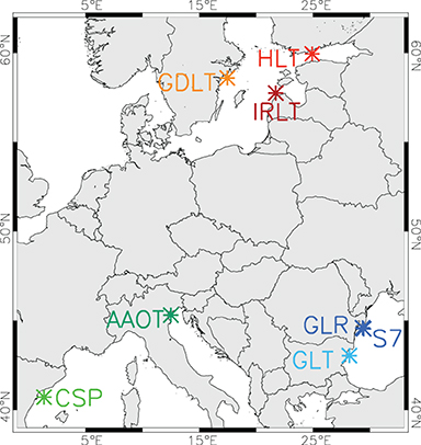
Figure 1. Maps of the AERONET-OC sites used in the analysis (see text for the definition of their acronyms).
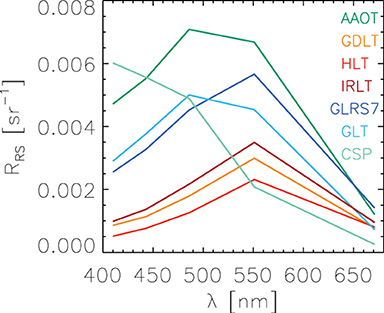
Figure 2. Average RRS spectra from PRS field data associated with VIIRS-SNPP match-ups. Acronyms refer to AERONET-OC sites (see text).
This study relied on AERONET-OC (version 3) data of multi-spectral normalized water-leaving radiance corrected for bidirectional effects using an IOP-based approach where the IOPs were computed using regional empirical algorithms (Zibordi et al., 2004, 2009). These data products were then converted in remote-sensing reflectance RRS by division by extra-terrestrial solar irradiance (Thuillier et al., 2003). Only level-2 RRS data having undergone the complete AERONET-OC quality control were used in this work. Relative uncertainties obtained for RRS at a site such as AAOT are ~5% at all bands except the red (~7%) (Zibordi et al., 2004) and tend to increase when RRS is in a lower range of values such as in Baltic waters (Gergely and Zibordi, 2014). Uncertainty values used in this work for PRS data are those expressed in radiometric units as defined by Gergely and Zibordi (2014).
2.2. Satellite Data
This study relied on the VIIRS data collected by the mission Suomi National Polar-orbiting Partnership (SNPP) launched in October 2011, and Joint Polar Satellite System (JPSS) -1 launched in November 2017 (Cao et al., 2013; Goldberg et al., 2013), which allows a current overlap of 3.5 years. Satellite Level-1A data for both VIIRS missions were acquired from the Ocean Biology Distributed Active Archive Center (OB.DAAC) of the National Aeronautics and Space Administration (NASA) and processed by the SeaWiFS Data Analysis System (SeaDAS, Fu et al., 1998) standard atmospheric correction (Gordon and Wang, 1994; Franz et al., 2007; Ahmad et al., 2010) according the latest NASA reprocessing option R2018. Besides being processed with the same code, both missions are also subject to the same strategy for system vicarious calibration (Franz et al., 2007), conditions that favor agreement between the products from the two missions. Nominal center-wavelengths for VIIRS on SNPP are given at 410, 443, 486, 551, and 671 nm, while they are 411, 445, 489, 556, and 667 nm for JPSS1.Thereafter, VIIRS-SNPP and VIIRS-JPSS1 are merely referred to as SNPP and JPSS1, respectively.
Macro-pixels of 3x3 pixels centered on each AERONET-OC site were then extracted from the Level-2 imagery. For each macro-pixel, field data registered less than 2 h from the satellite overpass, if any, were first selected. If field measurement records were available before and after the satellite overpass, then a weighted average was computed for the time of overpass using the two closest measurements found before and after the overpass; otherwise the closest measurement was adopted as the PRS field value. The maximum time difference allowed for the analysis (2 h) is in the continuity of past studies at the AERONET-OC sites (e.g., Zibordi et al., 2009). Considering their coastal, possibly more dynamic, character, it is lower than those adopted in studies more focused on the open ocean (e.g., 3 h, Bailey and Werdell, 2006).
Macro-pixels were excluded from the analysis if one pixel was affected by the standard level-2 flags of the SeaDAS processor applied when building level-3 products2, to the exception of the flag signaling coccolithophores, the presence of which can be recurrent in the Black Sea but that does not appear to degrade the performance of the atmospheric correction (Cazzaniga et al., 2021). Standard flags excluded all conditions leading to a failure or non-application of the atmospheric correction (such as cloudy conditions, high glint, influence of stray light) and large zenith angles for the illumination and observation directions. Furthermore, match-ups were ignored if the coefficient of variation (CV, ratio of standard deviation and average over the macro-pixel) calculated on RRS at selected wavelengths (486/489 and 551/556 nm) is larger than 0.2 to avoid spatially heterogeneous conditions. When comparing data from both VIIRS missions, the protocol selecting valid macro-pixels was similar, keeping inter-mission match-ups when the satellite overpass did not exceed 2 h (in practice all inter-mission match-ups were separated by less than 1 h).
Besides slightly different acquisition times, the comparison between satellite and field data is beset by a mismatch in spatial scales (pixel-size vs. point-based), which leads to a representation error (Oke and Sakov, 2008). As said above, heterogeneous conditions at the scale of the 3x3 macro-pixels were excluded with a test on CV. To further reduce the representation error, the satellite value compared with field data was computed at the position of the measurement site with a bilinear interpolation of the values associated with the four closest pixels surrounding its location, and the associated local variability was quantified by the standard deviation found for the four pixel values. Using Landsat-8 high-resolution data, Pahlevan et al. (2016) recommended using the closest pixel, while recognizing that other factors (striping or noise) could then adversely affect the comparison, so that the adopted approach appears as a good compromise. In practice, validation statistics are barely affected when using a 3x3-pixel average or the 2x2-pixel interpolation.
As far as a satellite-to-satellite comparison is concerned, Pahlevan et al. (2016) recommended a 7x7-km window size with size actually varying according to the selected area, but their decision criterion was fairly strict. Moreover the window size might be diversely translated in number of pixels for VIIRS (pixel size at nadir of ~0.75-km) with respect to a sensor such as the Moderate Resolution Spectroradiometer (MODIS, ~1-km). Considering also that the studied sites are in coastal waters, selecting a 3x3-pixel window rather than a larger one seemed safer to avoid potential adjacency effects (Bulgarelli and Zibordi, 2018).
Comparison between field and VIIRS data or between the two VIIRS missions was conducted at corresponding center-wavelengths but these may somewhat differ. Differences in center-wavelengths were corrected by a band-shifting scheme based on regional bio-optical relationships following Zibordi et al. (2009). In practice field data were expressed at the closest VIIRS center-wavelengths. The inter-mission comparison was made with three options, expressing RRS from SNPP at the nominal center-wavelengths of JPSS1, expressing RRS from JPSS1 at the nominal center-wavelengths of SNPP, and without performing any band shifting. It is anticipated that the choice of option barely affected comparison statistics.
2.3. Comparison Statistics
Considering a set of N match-ups with (xi)i = 1, N and (yi)i = 1, N, the PRS field data and satellite products, respectively, the following comparison metrics were introduced (Mélin and Franz, 2014; IOCCG, 2019):
with the overline indicating an average value. Δ, the root-mean-square (RMS) difference between x and y, can be decomposed by a development of squares into the average difference δ and a centered RMS difference Δc that is free from systematic effects. Δ and δ were also computed for the differences between SNPP and JPSS1 and are noted ΔVRS and δVRS (JPSS1 minus SNPP).
Relative differences were expressed with the following definitions:
for the median absolute relative difference |ψ|m and the median relative difference ψm, where the choice of the “median” operator was made to avoid the impact of outliers when the denominator was nearing 0.
Similar equations were used to compute differences between the two satellite products (SNPP and JPSS1). When applied to satellite data, relative differences were written in their unbiased (also called symmetric) form (taking the average of x and y as a reference, Armstrong, 1985; Mélin and Franz, 2014):
2.4. Error Model
Assuming a general approximate linear relationship between the distributions of the field data x and their satellite equivalent y (as supported by validation results, e.g., Bailey and Werdell, 2006; Zibordi et al., 2009; Mélin et al., 2011; Moore et al., 2015), a linear error model was adopted:
The field data x were written as the sum of a target reference state t and a zero-mean random error term ξ (random being here understood as uncorrelated with other quantities). The relationship between the reference t and the true value is undefined with the proviso that non-systematic effects are captured by ξ; in practice t only served as a link between x and y. Similarly, the satellite data y were written as a function of t with additive and multiplicative biases, α and β, respectively, and a zero-mean random error ϵ. It can be noted that the bias δ introduced by Equation (2) is equal to .
In this framework, the standard deviation of (ξi)i = 1, N, σξ, was assumed equal to the standard uncertainty defined for the field data (and therefore known, see section 2.1), and the objective was to define the terms characterizing the uncertainty budget of the satellite data y, particularly the term related to random effects quantified by the standard deviation of (ϵi)i = 1, N, σϵ.
Writing the variance and covariance terms , and σxy from Equations (8) and (9) leads to:
taking advantage of the fact that covariance terms with ξ or ϵ are equal to 0. A similar framework was applied by Mélin et al. (2016) to the case of two satellite data sets, where the system of equations was solved by assuming known the ratio between σξ and σϵ. Here instead, the system can be solved to calculate σϵ knowing σξ, which leads to:
From this equation, σϵ is a decreasing function of σξ, having as maximum , i.e., where r is the Pearson correlation coefficient between x and y. Equation (13) is only valid with a data set having a significant range of variability (σx>σξ).
For completeness, the value of the slope β is also given (model II regression, Legendre and Legendre, 1998):
noting γ=σϵ/σξ. If γ is very large (in situ data considered error-free and σξ=0), β is the slope of an ordinary least-square regression σxy/. Differently if γ = 1 (field and satellite data characterized by the same level of non-systematic effects in their uncertainty), β is the slope of a major axis regression (Legendre and Legendre, 1998).
The centered RMS difference Δc between field and satellite data can also be linked to the terms β, σϵ, and σξ (by considering that is the variance of (yi − xi)i = 1, N and therefore a combination of the three terms defined by Equations 10 to 12):
It can be noticed that is close to +, i.e., the sum, in variance space, of the uncertainty terms associated with random effects, only if β is close to 1. In the same way, putting aside systematic differences (biases) and assuming field data as error-free (σξ=0), then the difference between field and satellite data Δc is equal to , and can be equated to the uncertainties associated with satellite data (as represented by σϵ) only if β is close to 1.
3. Results
3.1. Validation Statistics
The comparison between VIIRS and PRS field data is shown for each site in Figure 3 for selected wavelengths while comparison statistics are given for the entire spectrum in Figures 4A,B for |ψ|m and ψm, and in Figures 5, 6 for Δ, Δc, and δ. More detailed statistics are given in Supplementary Material. The number of match-ups varies extensively from 684 at AAOT to 58 at IRLT for SNPP, and from 245 at AAOT to 32 at HLT for JPSS1. Besides the fact that SNPP has been in orbit for a longer period than JPSS1, the number of match-ups obviously depends on the environmental conditions encountered at each site as well as on the periods of operation of the PRS systems. For instance there are no match-ups for the Baltic sites in the winter period and the site of HLT was not active in 2018 and 2020, explaining the low number of match-ups for JPSS1.
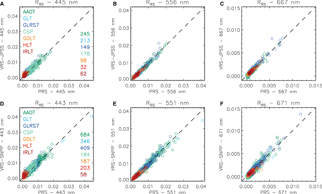
Figure 3. Scatter plots of RRS match-ups with respect to AERONET-OC PRS data for VIIRS-JPSS1 (A–C) and VIIRS-SNPP (D–F) at selected wavelengths. Acronyms refer to AERONET-OC sites (see text). Numbers indicate the number of match-ups for each site.
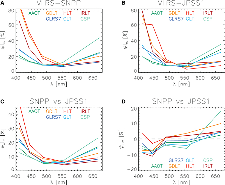
Figure 4. For the various AERONET-OC sites: spectra of median absolute relative difference |ψ|m for (A) the comparison between PRS and VIIRS-SNPP data and for (B) the comparison between PRS and VIIRS-JPSS1; spectra of (C) median unbiased absolute relative difference |ψu|m and (D) median unbiased relative difference ψu, m for the comparison between VIIRS-JPSS1 and VIIRS-SNPP data.
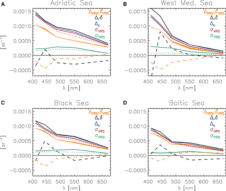
Figure 5. Spectra of statistical quantities for VIIRS-SNPP for sites in (A) the Adriatic Sea, (B) the Western Mediterranean Sea, (C) the Black Sea, and (D) the Baltic Sea. Comparing SNPP and PRS field data: Δ is the RMS difference (solid line), δ is the average difference (dashed line) and Δc is the centered RMS difference. Comparing VIIRS SNPP and JPSS1 data, ΔPRS is the RMS difference (sold line), δVRS is the average difference (dashed line, JPSS1-SNPP). σPRS is the uncertainty associated with PRS field data (solid green line); the average standard deviation of the measurements used for each match-up is shown with a dotted green line. σVRS is the SNPP uncertainty term associated with random effects, without and with correction for representation error (solid and dotted lines, respectively). Note that ΔVRS and δVRS are equally represented in Figure 6.
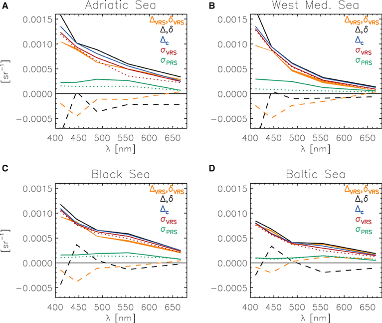
Figure 6. Spectra of statistical quantities for VIIRS-JPSS1 for sites in (A) the Adriatic Sea, (B) the Western Mediterranean Sea, (C) the Black Sea, and (D) the Baltic Sea. Comparing JPSS1 and PRS field data: Δ is the RMS difference (solid line), δ is the average difference (dashed line) and Δc is the centered RMS difference. Comparing VIIRS SNPP and JPSS1 data, ΔPRS is the RMS difference (sold line), δVRS is the average difference (dashed line, JPSS1-SNPP). σPRS is the uncertainty associated with PRS field data (solid green line); the average standard deviation of the measurements used for each match-up is shown with a dotted green line. σVRS is the JPSS1 uncertainty term associated with random effects, without and with correction for representation error (solid and dotted lines, respectively). Note that ΔVRS and δVRS are equally represented in Figure 5.
Validation results appear well consistent for both VIIRS missions (as well as with previous missions; e.g., Zibordi et al., 2009, 2015; Mélin et al., 2012), with match-up points fairly well-distributed along the 1:1 line when all sites are considered (Figure 3). The maximum values of RRS are associated with conditions of coccolithophore blooms in the Black Sea (Cazzaniga et al., 2021). The median absolute relative difference |ψ|m show the expected U shape for this type of metrics (e.g., Mélin and Franz, 2014) with larger values for the blue or red bands when the RRS values are low (Figures 4A,B). This is obviously the case for Baltic waters that are highly absorbing with low RRS in the blue (see Figure 2) and |ψ|m above 60% at 410/411 nm for both SNPP and JPSS1. To the contrary, the CSP site with fairly clear waters is characterized by low RRS in the red (671/667 nm) and the highest |ψ|m in that spectral region (44% and 35% for SNPP and JPSS1, respectively). For the two Black Sea sites (GLRS7 and GLT), |ψ|m is approximately 30 and 20% for the first two bands while it is lower at AAOT and CSP (~21% and 12–14%). For SNPP at 551 nm, |ψ|m varies in the interval 7–10% for all sites (except 12% at CSP), and for JPSS1 at 556 nm in the interval 7–11% (except 4% at HLT). At 486/489 nm, |ψ|m is also lower than 10% for AAOT, CSP and the Black Sea sites. In the red, |ψ|m is in the interval 9–15% for the Baltic sites (except 20% at GDLT for SNPP). Considering the similar properties and validation results and for ease of presentation, the match-ups of the three Baltic Sea sites are grouped to compute uncertainty statistics; the same procedure is carried out with the two Black Sea sites. This also reinforces the statistical significance of the results by increasing the sample size.
When expressed in radiometric units, statistics tend to be closer among the sites (Figures 5, 6), with the RMS difference Δ decreasing regularly with wavelength from an interval among all sites of 0.76–1.7 10−3 sr−1 at 410/411 nm to 0.14–0.41 10−3 sr−1 at 671/667 nm. The AAOT and CSP sites are characterized by the highest Δ in the blue, while the Baltic sites have the lowest values. When looking at the bias δ, a clear agreement between sites and missions can be noted: δ tends to be negative at 410/411 nm (with a value as large as −0.001 sr−1 for JPSS1 at CSP) and positive at 443/445 nm, illustrating a certain spectral inconsistency for these two bands. Above 486 nm, δ is in the interval ±0.3 10−3 sr−1 (and most often ±0.2 10−3 sr−1). The centered RMS difference Δc is mostly very close to Δ except for the cases where δ is largely negative, at CSP in the blue for both VIIRS missions, and at AAOT for JPSS1.
As far as the multiplicative bias is concerned, β is mostly in the interval 0.8–1.1, except lower values at 410 nm for SNPP for the Baltic sites (0.35) and in the red at CSP (~0.6). This indicates that the first term in the expression of Δc [proportional to (β−1)2, Equation 15] is usually fairly small.
3.2. Inter-mission Comparison
Using the period of mission overlap, Figure 7 shows the direct comparison between SNPP and JPSS1 RRS that confirms the fair agreement between the two missions anticipated from the validation statistics. As mentioned in section 2.2, the comparison between the two missions was made with three cases: without band-shifting (keeping RRS unchanged) and after application of a band-shifting expressing SNPP RRS at the JPSS1 bands, or JPSS1 RRS at the SNPP bands. Comparison statistics change very little with these three cases. For instance, Figures 5, 6 show the RMS difference ΔVRS as an envelop defined by the maximum and minimum ΔVRS obtained for the three cases at each wavelength: it is barely distinguishable from a single thick line. From now onward, only the case without band-shifting is discussed. It is however stressed that the application of a band-shifting scheme might be required for other pairs of sensors and/or other water types.
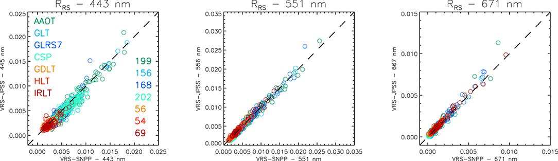
Figure 7. Scatter plots of VIIRS-JPSS1 RRS data with respect to VIIRS-SNPP RRS at selected wavelengths.
Figures 4C,D provides the median (unbiased) relative differences |ψu|m and ψu, m for the various sites. Again, a U shape is seen for |ψu|m with high values in the blue or red bands when RRS is low: at 410/411 nm, |ψu|m is higher than 30% for the Baltic sites (up to 48% at HLT), and 23% at 671/667 nm for CSP. To the contrary, the lowest |ψu|m in the red is found at IRLT (7%), GLR (8%), and HLT (9%), and at 410/411 nm at CSP (13%). The agreement is encouraging at 486/489 and 551/556 nm, with |ψu|m always lower than 10% (and often lower than 7%). The relative bias (JPSS1 values minus SNPP values) tends to increase with wavelength, from usually between −4 and −10% at 410/411 and 443/445 nm to positive values in the red. When expressed in radiometric units, the mean difference δVRS is also usually negative in the blue (i.e., JPSS1 RRS lower) and lower (in modulus) than 0.2 10−3 sr−1, except at 443/445 nm where δVRS can be as low as −0.5 10−3 sr−1 (Figures 5, 6).
The RMS difference ΔVRS between SNPP and JPSS1 RRS, illustrated in Figures 5, 6, shows a regular decrease with wavelength, fairly parallel to Δ. At AAOT, CSP and the Black Sea sites, ΔVRS is 0.9–1 10−3 sr−1, and is slightly lower at the Baltic site (0.76 10−3 sr−1). In the red, ΔVRS is increasing from CSP (0.06 10−3 sr−1), the Baltic sites (0.17 10−3 sr−1), the Black Sea sites (0.22 10−3 sr−1) to AAOT (0.29 10−3 sr−1). In general, ΔVRS is clearly lower than Δ (RMS difference with respect to field data) except at the Baltic sites when Δ is computed for JPSS1 (Figure 6D).
3.3. Uncertainties of the Satellite Products
Following the framework introduced in section 2.4, the uncertainty term associated with random effects was computed with Equation (13) and is here noted σVRS for the VIIRS products (or σSNPP and σJPSS1 when specific to a sensor) and σPRS for the PRS field data (equivalent to σϵ and σξ in section 2.4).
As seen in Figures 5, 6 and Supplementary Material, σVRS decreases with wavelengths for both VIIRS missions and all regions. At 410/411 nm, it is found in the interval 1.2–1.4 10−3 sr−1 at 410/411 nm for the northern Adriatic and western Mediterranean areas (AAOT and CSP), slightly lower for the Black Sea sites (~1.1 10−3 sr−1) and lowest for the Baltic sites (0.8–0.9 10−3 sr−1). In the green, AAOT and the Black Sea sites have the highest values of σVRS (0.5–0.8 10−3 sr−1), while it is lower for CSP and the Baltic sites (~0.3 10−3 sr−1). In the red, it is highest for AAOT (0.2–0.3 10−3 sr−1), lower for Baltic and Black Sea sites (0.15–0.25 10−3 sr−1) and lowest (<0.1 10−3 sr−1) at CSP, a site where RRS is low. An important result is that σSNPP and σJPSS1 are close to each other. Considering the four regions and the five bands, the ratio σJPSS1/σSNPP is mostly in the interval 0.8–1.05 (except in the green and red bands at AAOT, where it is ~0.7), with σJPSS1 lower in almost all cases. Besides possible differences between the two missions, differences in σVRS can be explained by the differing number of match-ups found for each mission. On the other hand, the general agreement (compare Figures 5, 6) is favored by the similar characteristics of the sensors and by the use of common algorithms to process their data.
The spectra of σVRS appear fairly close to Δc, which, considering Equation (15), is explained by the relatively low values of σPRS and values of β not far from 1. σPRS is always lower than 0.3 10−3 sr−1, a value reached in the green at AAOT and in the blue for CSP (in association with relatively high values of RRS). Considering that σVRS is clearly higher than σPRS and that the uncertainties associated with PRS data are at least 5% when expressed in relative terms (Gergely and Zibordi, 2014), the VIIRS RRS products at the considered sites do not comply with an objective of a 5% uncertainty advocated by the Global Climate Observing System (GCOS, 2011). It is however fair to recall that the AERONET-OC sites are located in coastal regions whereas this 5% objective applies to open ocean waters, and that even in these conditions, it might not be currently fulfilled for all bands (Hu et al., 2013; Mélin et al., 2016).
There are no readily available independent estimates of uncertainty for RRS that could serve as a point of comparison with the present results. Hu et al. (2013) provide uncertainties for SeaWiFS and MODIS (Moderate Resolution Imaging Spectroradiometer) RRS data by looking at the deviations of RRS with respect to reference values defined in relation to a reference chlorophyll-a algorithm (Hu et al., 2012). This approach is only applicable in oligotrophic waters, conditions which are usually not observed at the AERONET-OC sites. However, considering that the CSP site is often associated with Case-1 waters, a comparison can be performed for completeness. For the highest chlorophyll-a concentration tabulated by Hu et al. (2013) (0.2 mg m−3 in the North Atlantic), uncertainty estimates in the blue (~412 nm) are much lower than σVRS at CSP: 0.68 10−3 sr−1 and 0.79 10−3 sr−1 for MODIS and SeaWiFS, respectively, vs. ~1.3 10−3 sr−1 for σVRS; on the other hand they are of the same order at the green band, ~0.3 10−3 sr−1.
4. Discussion and Conclusion
In metrological analyses, the definition of uncertainties typically relies on repeating a given measurement in well-controlled conditions, a context that is not applicable for Earth observation remote sensing where each pixel is observed only once. The determination of uncertainty estimates for satellite products on the basis of a set of match-ups distributed in time and associated with varying observation conditions is, in that regard, an extension of metrological practices and can only provide a generic value for the match-up data set as a whole, while the actual uncertainty may vary from one match-up to another. In fact, validation statistics or inter-mission comparisons have shown temporal (e.g., seasonal) variations (Mélin et al., 2009, 2016; Zibordi et al., 2012; Bisson et al., 2021). Acknowledging this proviso, but considering the lack of alternative, a mathematical framework has been introduced to define an uncertainty budget for the VIIRS RRS products in term of random effects (σVRS) and systematic effects (β and α, or alternatively δ).
A first point worth discussing is the representation error, mentioned in section 2.2, that quantifies the discrepancy associated with the comparison of field data and satellite products: the satellite measurement imperfectly represents the field observation because of a different spatial scale, a different time of acquisition and possibly a different wavelength. In the framework introduced by Equations (8) and (9), the representation error is not explicitly defined, possibly leading to an overestimate of the uncertainties σVRS of the VIIRS products. Assuming effects as non-systematic and uncorrelated with measured values, the latter two points (different times of measurement and wavelengths) can be taken as part of the term ξ in Equation (8), leading to an increase in σξ (i.e., σPRS) that becomes the uncertainty of a virtual field measurement that would have been taken at the time of the satellite overpass and at a VIIRS wavelength (it is recalled that the comparison between field observations and satellite data is carried out at the satellite bands and that therefore the band-shifting is applied to the former). In turn this leads to a decrease in σϵ (σVRS) through Equation (13).
As far as differences in wavelengths are concerned, uncertainties due to band-shifting with an IOP-based technique depends much on the spectral distance between input and target wavelengths as well as the water type, and should not exceed a few percent (Mélin and Sclep, 2015). As a measure of temporal variability, the standard deviation between the two PRS observations registered before and after the satellite overpass is comparable to PRS uncertainties for the Baltic sites, and is lower for the other regions (and in line with the few-% variability documented for AAOT, Zibordi et al., 2006; Mélin and Zibordi, 2007), the minimum being seen at the western Mediterranean CSP site characterized by water stability (dotted green lines in Figures 5, 6). Therefore, differences between two successive PRS measurements can be at least partly explained by their inherent uncertainties, so that the extent to which this variability can be interpreted as estimates of the uncertainty contributions due to different times of acquisition is unclear. Additionally, for the match-ups where two field observations were available (preceding and following the overpass), an interpolated value was computed (section 2.2), which should reduce this contribution, but only if the RRS evolution between the two acquisition times is regular. The availability of two field observations is met for ~60% of the match-ups, the others relying on only one PRS value separated (before or after) from the satellite overpass by on average ~44±32 min. Eventually, no correction is attempted for this effect, pending dedicated analyses on complete PRS data series.
It should also be kept in mind that temporal and spatial variability are not easily untangled. For the sake of discussion, we will focus on the latter and assume that it is the main contributor to the representation error associated with the satellite products (thus also termed collocation error). Again assuming the effects related to spatial variability as non-systematic and uncorrelated with measured values, they can be considered part of the term ϵ in Equation (9). The uncertainties σVRS of the VIIRS products described in section 3.3 can thus be corrected for a representation error of variance , following:
Here the representation error is approximated by the inter-pixel variability taken as a measure of local variability and computed as the quadratic average over the match-ups of the standard deviation among the 2x2 pixels used to derive the satellite match-up value. The resulting shown in Figures 5, 6 (dotted line) is only slightly below σVRS suggesting that the representation error does not have a large impact on the estimate of the uncertainty. There are, however, exceptions such as at AAOT for 551/556 nm, where a significant decrease can be seen between σVRS and . The inter-pixel standard deviation is on average 2–5% of RRS, with larger values for cases of low RRS, for instance rising at 410/411 nm to ~8% at the Black Sea sites and ~16% at the Baltic sites, and in the red (typically 7–9%, up to 23% for CSP and SNPP). Using high-resolution satellite data, Pahlevan et al. (2016) concluded that discrepancies due to spatial sampling are for selected validation sites in the interval 2–4% on average, with higher values in some cases (as high as 18%), so that intra-pixel variability (that would be the quantity to prefer when estimating the representation error) is in general slightly lower than the inter-pixel variability used here. While acknowledging that a more detailed analysis would be required on this issue, the actual value of the uncertainty for VIIRS products is likely to be between σVRS and , which again would indicate a fairly small contribution from the representation error in the uncertainty budget.
The second point of discussion is to qualify the differences observed between the VIIRS missions taking into account their uncertainties. In metrological terms, this means assessing their compatibility, that is to say how, for any pair of VIIRS products, their difference (in modulus) compares with some chosen multiple (a coverage factor k) of the uncertainty of the difference udif (VIM, 2012). This leads to quantify the occurrence of the following expression (e.g., Immler et al., 2010; Calbet et al., 2017):
Considering the four regions and all bands, this statement is true for k=1 for a fraction of the match-ups larger than 80% (often larger than 90%), suggesting that the data from the two missions are indeed compatible, i.e., that they agree within their stated uncertainties. This result could be anticipated by observing that ΔVRS, the RMS difference between SNPP and JPSS1 RRS is usually comparable to, or lower than, σVRS (Figures 5, 6).
However, Equation (17) is valid only if the errors eSNPP and eJPSS1 associated with SNPP and JPSS1, respectively, are uncorrelated. In the opposite case, Equation (17) should be rewritten as:
where r(.) is the correlation operator (GUM, 2008).
Considering that the uncertainty associated with field observations are well below those of VIIRS data, it may be assumed that this correlation of errors can be approximated by the correlation between residuals associated with the two missions, where residuals are defined as differences between satellite and field data:
Figure 8 shows spectra of the correlation between residuals computed with the match-up data common to both VIIRS missions. The results obtained for HLT indicate a very low correlation in the blue bands and values larger than 0.5 only in the green and red bands. It is however noted that the number of common match-ups is small (24) with a small dynamic range in the blue bands. For sites with a more sizable common match-up set (including the other two Baltic locations), the correlation coefficient is almost always in the interval 0.55-0.8, which is simply interpreted as follows: for a given day, if the difference between SNPP and PRS RRS is above its average value, the difference between JPSS1 and PRS RRS tends to be larger than its average value too. This behavior is easily explained by the fact that the two sensors share a common design and their data are processed with the same strategy for calibration (including system vicarious calibration) and atmospheric correction and associated algorithms.
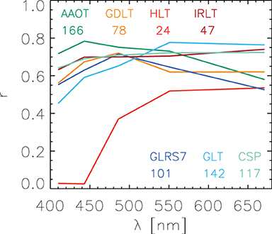
Figure 8. Spectra of correlation coefficient between residuals of VIIRS SNPP and JPSS1 (i.e., differences with respect to PRS field data) computed with common match-ups.
Considering all bands and the five sites with a sufficient number of match-ups (AAOT, CSP, GDLT, GLRS7 and GLT), the fraction of match-ups satisfying Equation (18) is still usually higher than 68% for a coverage factor k=1, and is mostly in the interval 0.85–0.99 for k=2 (85% for 551/556 nm at HLT, 75–79% for green and red bands at IRLT), indicating that the diagnostic of compatibility still stands, albeit with a reduced significance.
As a final note, the agreement between the two missions can also be discussed in a context of climate science looking at the concentration of chlorophyll-a (Chl-a), an Essential Climate Variable according to GCOS (2011). Match-ups between SNPP and JPSS1 indicate a relative difference (bias) in Chl-a of ~5% at AAOT and CSP, 3–8% at the Black Sea sites and more than 17% at the Baltic sites. As a consequence, aggregating Chl-a data from the two missions without correcting for these differences might create spurious trends in data analyses (Mélin, 2016). This being said, the agreement shown between the two missions in terms of RRS and Chl-a appears already suitable for less demanding applications.
In conclusion, this study has presented a framework to interpret validation statistics in terms of uncertainties for the satellite products knowing the uncertainties associated with the field data. This framework has been applied to the first two elements of the VIIRS series (SNPP and JPSS1) that show similar estimates of uncertainties σVRS (term accounting for non-systematic contributions to the uncertainty budget), decreasing with wavelength from the interval 0.8–1.4 10−3 sr−1 in the blue to a maximum of 0.24 10−3 sr−1 in the red, values that are at least twice (but up to 8 times) the uncertainties reported for the field data. These uncertainty estimates have allowed an informed assessment of the differences between the two VIIRS RRS products that finds them fairly compatible, even when error correlations are duly accounted for. Of course, this approach can be applied to other products from different missions and/or agencies and to other derived quantities. On the other hand, the proposed framework requires a significant amount of fully-characterized field data to gather a sufficient number of match-ups suitable for statistical analysis. It also provides only one aggregate value for the entire data set and can not give uncertainty estimates for each match-up. But the results presented here for specific sites will be needed to verify pixel-based uncertainty estimates derived by other means (IOCCG, 2019) and can be useful to investigate the propagation of RRS uncertainties through bio-optical algorithms (McKinna et al., 2019). They are therefore much needed for a thorough evaluation of the ocean color data record.
Data Availability Statement
Publicly available datasets were analyzed in this study. These data can be found here: https://aeronet.gsfc.nasa.gov; https://oceancolor.gsfc.nasa.gov.
Author Contributions
The author confirms being the sole contributor of this work and has approved it for publication.
Funding
Partial funding was given by the EMPIR grant 19ENV07 associated with the MetEOC-4 project under the EMPIR programme.
Conflict of Interest
The author declares that the research was conducted in the absence of any commercial or financial relationships that could be construed as a potential conflict of interest.
Publisher's Note
All claims expressed in this article are solely those of the authors and do not necessarily represent those of their affiliated organizations, or those of the publisher, the editors and the reviewers. Any product that may be evaluated in this article, or claim that may be made by its manufacturer, is not guaranteed or endorsed by the publisher.
Acknowledgments
The author gratefully acknowledge funding from the MetEOC-4 project (in turn funded under EMPIR grant 19ENV07). The EMPIR programme is co-financed by the Participating States and from the European Union's Horizon 2020 research and innovation programme. The Ocean Biology Distributed Active Archive Center (OB.DAAC) of NASA is acknowledged for the distribution of the VIIRS Level-1 data. Giuseppe Zibordi is warmly thanked for his considerable efforts in ensuring the operations of the AERONET-OC sites.
Supplementary Material
The Supplementary Material for this article can be found online at: https://www.frontiersin.org/articles/10.3389/fmars.2021.790948/full#supplementary-material
Footnotes
1. ^Standing for Sea-viewing Wide Field-of-view Sensor.
References
Ahmad, Z., Franz, B., McClain, C., Kwiatkowska, E., Werdell, P., Shettle, E., et al. (2010). New aerosol models for the retrieval of aerosol optical thickness and normalized water-leaving radiances from the SeaWiFS and modis sensors over coastal regions and open oceans. Appl. Opt. 49, 5545–5560. doi: 10.1364/AO.49.005545
Armstrong, J.. (1985). Long-Range Forecasting: From Crystal Ball to Computer, 2nd Edn. New York, NY: Wiley.
Bailey, S., and Werdell, P. (2006). A multi-sensor approach for the on-orbit validation of ocean color satellite data products. Remote Sens. Environ. 102, 12–23. doi: 10.1016/j.rse.2006.01.015
Bisson, K., Boss, E., Werdell, P., Ibrahim, A., Frouin, R., and Behrenfeld, M. (2021). Seasonal bias in global ocean color observations. Appl. Opt. 60, 6978–6988. doi: 10.1364/AO.426137
Bulgarelli, B., and Zibordi, G. (2018). On the detectability of adjacency effects in ocean color remote sensing of mid-latitude coastal environments by SeaWiFS, MODIS-A, MERIS, OLCI, OLI and MSI. Remote Sens. Environ. 209, 423–438. doi: 10.1016/j.rse.2017.12.021
Calbet, X., Peinado-Galan, N., Rípodas, P., Trent, T., Dirksen, R., and Sommer, M. (2017). Consistency between GRUAN sondes, LBLRTM and IASI. Atmos. Meas. Tech. 10, 2323–2335. doi: 10.5194/amt-10-2323-2017
Cao, C., Xiong, J., Blonski, S., Liu, Q., Uprety, S., Shao, X., et al. (2013). Suomi NPP VIIRS sensor data record verification, validation, and long-term performance monitoring. J. Geophys. Res. 118, 11664–11678. doi: 10.1002/2013JD020418
Cazzaniga, I., Zibordi, G., and Mélin, F. (2021). Spectral variations of the remote sensing reflectance during coccolithophore blooms in the western Black sea. Remote Sens. Environ. 264:112607. doi: 10.1016/j.rse.2021.112607
Donlon, C., Berruti, B., Buongiorno, A., Ferreira, M.-H., Féménias, P., Frerick, J., et al. (2012). The global monitoring for environment and security (GMES) sentinel-3 mission. Remote Sens. Environ. 120, 37–57. doi: 10.1016/j.rse.2011.07.024
Franz, B., Bailey, S., Werdell, P., and McClain, C. (2007). Sensor-independent approach to the vicarious calibration of satellite ocean color radiometry. Appl. Opt. 46, 5068–5082. doi: 10.1364/AO.46.005068
Fu, G., Baith, K., and McClain, C. (1998). “SeaDAS: the SeaWIFS data analysis system,” in Proceedings of the 4th Pacific Ocean Remote Sensing Conference (Qingdao), 73–79.
GCOS (2011). Systematic Observation Requirements for Satellite-Based Products for Climate. GCOS-154, Supplemental details to the satellite-based component of the “Implementation plan for the Global Observing System for Climate in Support of the UNFCC”.
Gergely, M., and Zibordi, G. (2014). Assessment of AERONET-OC LWN uncertainties. Metrologia 51, 40–47. doi: 10.1088/0026-1394/51/1/40
Goldberg, M. D., Kilcoyne, H., Cikanek, H., and Mehta, A. (2013). Joint polar satellite system: the United States next generation civilian polar-orbiting environmental satellite system. J. Geophys. Res. 118, 13463–13475. doi: 10.1002/2013JD020389
Gordon, H., Clark, D., Brown, J., Brown, O., Evans, R., and Broenkow, W. (1983). Phytoplankton pigment concentrations in the Middle Atlantic Bight: comparison between ship determinations and coastal zone color scanner estimates. Appl. Opt. 22, 20–36. doi: 10.1364/AO.22.000020
Gordon, H., and Wang, M. (1994). Retrieval of water-leaving radiance and aerosol optical thickness over the oceans with SeaWiFS: a preliminary algorithm. Appl. Opt. 33, 443–452. doi: 10.1364/AO.33.000443
GUM (2008). Evaluation of Measurement Data–Guide to the Expression of Uncertainty in Measurements. Joint Committee for Guides in Metrology, Bureau International des Poids et Mesures.
Hu, C., Feng, L., and Lee, Z.-P. (2013). Uncertainties of SeaWiFS and MODIS remote sensing reflectance: implications from clear water measurements. Remote Sens. Environ. 133, 163–182. doi: 10.1016/j.rse.2013.02.012
Hu, C., Lee, Z.-P., and Franz, B. (2012). Chlorophyll a algorithms for oligotrophic oceans: a novel approach based on three-band reflectance difference. J. Geophys. Res. 117:C01011. doi: 10.1029/2011JC007395
Immler, F., Dykema, J., Gardiner, T., Whiteman, D., Thorne, P., and Vömel, H. (2010). Reference quality upper-air measurements: guidance for developing GRUAN data products. Atmos. Meas. Tech. 3, 1217–1231. doi: 10.5194/amt-3-1217-2010
IOCCG (2019). Uncertainties in Ocean Colour Remote Sensing. Reports of the International Ocean Colour Coordinating Group. IOCCG, Dartmouth, NS, Canada.
McKinna, L., Cetinić, I., Chase, A., and Werdell, P. (2019). Approach for propagating radiometric data uncertainties through NASA ocean color algorithms. Frontiers Earth Sci. 7:176. doi: 10.3389/feart.2019.00176
Mélin, F.. (2016). Impact of inter-mission differences and drifts on chlorophyll-a trend estimates. Int. J. Remote Sens. 37, 2061–2079. doi: 10.1080/01431161.2016.1168949
Mélin, F., and Franz, B. (2014). “Assessment of satellite ocean colour radiometry and derived geophysical products,” in Optical Radiometry for Oceans Climate Measurements, eds G. Zibordi, C. Donlon, and A. Parr (San Diego, CA: Academic Press), 609–638. doi: 10.1016/B978-0-12-417011-7.00020-9
Mélin, F., and Sclep, G. (2015). Band-shifting for ocean color multi-spectral reflectance data. Opt. Exp. 23, 2262–2279. doi: 10.1364/OE.23.002262
Mélin, F., Sclep, G., Jackson, T., and Sathyendranath, S. (2016). Uncertainty estimates of remote sensing reflectance derived from comparison of ocean color satellite data sets. Remote Sens. Environ. 177, 107–124. doi: 10.1016/j.rse.2016.02.014
Mélin, F., and Zibordi, G. (2007). Optically based technique for producing merged spectra of water-leaving radiances from ocean color remote sensing. Appl. Opt. 46, 3856–3869. doi: 10.1364/AO.46.003856
Mélin, F., Zibordi, G., and Berthon, J.-F. (2012). Uncertainties in remote sensing reflectance from MODIS-Terra. IEEE Geosci. Remote Sens. Lett. 9, 432–436. doi: 10.1109/LGRS.2011.2170659
Mélin, F., Zibordi, G., Berthon, J.-F., Bailey, S., Franz, B., Voss, K., et al. (2011). Assessment of MERIS reflectance data as processed by SeaDAS over the european seas. Opt. Exp. 19, 25657–25671. doi: 10.1364/OE.19.025657
Mélin, F., Zibordi, G., and Djavidnia, D. (2009). Merged series of normalized water leaving radiances obtained from multiple satellite missions for the mediterranean sea. Adv. Space Res. 43, 423–437. doi: 10.1016/j.asr.2008.04.004
Moore, T., Campbell, J., and Feng, H. (2015). Characterizing the uncertainties in spectral remote sensing reflectance for SeaWiFS and MODIS-Aqua based on global in situ matchup data sets. Remote Sens. Environ. 159, 14–27. doi: 10.1016/j.rse.2014.11.025
Oke, P., and Sakov, P. (2008). Representation error of oceanic observations for data assimilation. J. Atmos. Ocean. Tech. 25, 1004–1017. doi: 10.1175/2007JTECHO558.1
Pahlevan, N., Sarkar, S., and Franz, B. (2016). Uncertainties in coastal ocean color products: impacts of spatial sampling. Remote Sens. Environ. 181, 14–26. doi: 10.1016/j.rse.2016.03.022
Thuillier, G., Hersé, M., Labs, D., Foujols, T., Peetermans, W., Gillotay, D., et al. (2003). The solar spectral irradiance from 200 to 2400 nm as measured by the SOLSPEC spectrometer from the ATLAS and Eureca missions. Sol. Phys. 214, 1–22. doi: 10.1023/A:1024048429145
VIM (2012). International Vocabulary of Metrology - Basic and General Concepts and Associated Terms. JCGM 200. Joint Committee for Guides in Metrology, Bureau International des Poids et Mesures.
Zibordi, G., Berthon, J.-F., Mélin, F., and D'Alimonte, D. (2011). Cross-site consistent in-situ measurements for satellite ocean color applications: the BiOMaP radiometric dataset. Remote Sens. Environ. 115, 2104–2115. doi: 10.1016/j.rse.2011.04.013
Zibordi, G., Berthon, J.-F., Mélin, F., D'Alimonte, D., and Kaitala, S. (2009). Validation of satellite ocean color primary products at optically complex coastal sites: Northern Adriatic Sea, Northern Baltic Proper, Gulf of Finland. Remote Sens. Environ. 113, 2574–2591. doi: 10.1016/j.rse.2009.07.013
Zibordi, G., Holben, B., Talone, M., D'Alimonte, D., Slutsker, I., Giles, D., et al. (2021). Advances in the ocean color component of the aerosol robotic network (AERONET-OC). J. Atmos. Ocean. Technol. 38, 725–746. doi: 10.1175/JTECH-D-20-0085.1
Zibordi, G., Mélin, F., and Berthon, J.-F. (2006). A time series of above-water radiometric measurements for coastal water monitoring and remote sensing product validation. IEEE Geosci. Remote Sens. Lett. 3, 120–124. doi: 10.1109/LGRS.2005.858486
Zibordi, G., Mélin, F., and Berthon, J.-F. (2012). Intra-annual variations of biases in remote sensing primary ocean color products at a coastal site. Remote Sens. Environ. 124, 627–636. doi: 10.1016/j.rse.2012.06.016
Zibordi, G., Mélin, F., Berthon, J.-F., and Talone, M. (2015). In situ autonomous optical radiometry measurements for satellite ocean color validation in the western Black Sea. Ocean Sci. 11, 275–286. doi: 10.5194/os-11-275-2015
Keywords: ocean color, uncertainties, validation, VIIRS, AERONET-OC
Citation: Mélin F (2021) From Validation Statistics to Uncertainty Estimates: Application to VIIRS Ocean Color Radiometric Products at European Coastal Locations. Front. Mar. Sci. 8:790948. doi: 10.3389/fmars.2021.790948
Received: 07 October 2021; Accepted: 22 November 2021;
Published: 23 December 2021.
Edited by:
Griet Neukermans, Ghent University, BelgiumReviewed by:
Lachlan McKinna, Go2Q Pty., Ltd., AustraliaLin Qi, University of South Florida, United States
Copyright © 2021 Mélin. This is an open-access article distributed under the terms of the Creative Commons Attribution License (CC BY). The use, distribution or reproduction in other forums is permitted, provided the original author(s) and the copyright owner(s) are credited and that the original publication in this journal is cited, in accordance with accepted academic practice. No use, distribution or reproduction is permitted which does not comply with these terms.
*Correspondence: Frédéric Mélin, ZnJlZGVyaWMubWVsaW5AZWMuZXVyb3BhLmV1