Assessments of Nitrate Budgets in the Yellow Sea Based on a 3D Physical-Biogeochemical Coupled Model

Nitrate (NO₃^–) plays an important role in ecosystems and aquaculture in the Yellow Sea (YS). Sparse observational data suggest that ocean currents and nitrification are crucial to NO₃^– flux in the YS; however, a quantitative assessment of these fluxes has not yet been performed. This study investigates seasonal and spatial variations in NO₃^– flux via currents and biological processes in the YS from 2006 to 2019 using a physical-biogeochemical coupled model. The model results show that the current-driven fluxes exceeded biological processes in the eastern and central regions of the YS, unlike in the western and northern regions. Advection of NO₃^– in the YS is mainly driven by cyclonic circulation in summer and fall, and anticyclonic circulation in spring and winter. The Subei Coastal Current along the coast of China plays a primary role in net advective influx of NO₃^– to the YS year round. The NO₃^– influx by the Yellow Sea Warm Current along the lower layer of the southcentral YS is offset by outflux through wind-driven surface currents in winter. The southward movements of the Yellow Sea Bottom Cold Water in summer and the Korean Coastal Current in winter are major NO₃^– outfluxes to the East China Sea. In terms of biological processes, NO₃^– is mainly consumed by phytoplankton during the spring bloom and supplied through organic matter decomposition and nitrification. Net supply of NO₃^– by biological processes was the greatest in the southcentral YS where the Yellow Sea Bottom Cold Water is present.

Introduction

The Yellow Sea (YS) in the Northwestern Pacific Ocean is a shallow, semi-enclosed marginal sea with an average depth of approximately 50 m and a deep trough (>90 m) in its center (Figure 1). The YS is a typical marginal sea with high primary productivity and rich fishery resources. Dissolved inorganic nitrogen (DIN) including nitrate (NO₃^–), nitrite (NO₂^–), and ammonium (NH₄⁺⁺) is critical in biological production and often a limiting factor in primary production in marine ecosystems (Ryther and Dunstan, 1971; Howarth, 1988). The fixed nitrogen in the YS is supplied by various sources including advection, rivers, atmospheric deposition, sediment flux, and nitrogen fixation (Bashkin et al., 2002; Kim et al., 2011; Kim S. K. et al., 2013). Previous studies reported that NO₃^–, accounting for approximately 87% of the total inorganic nitrogen in the YS, is the most

FIGURE 1

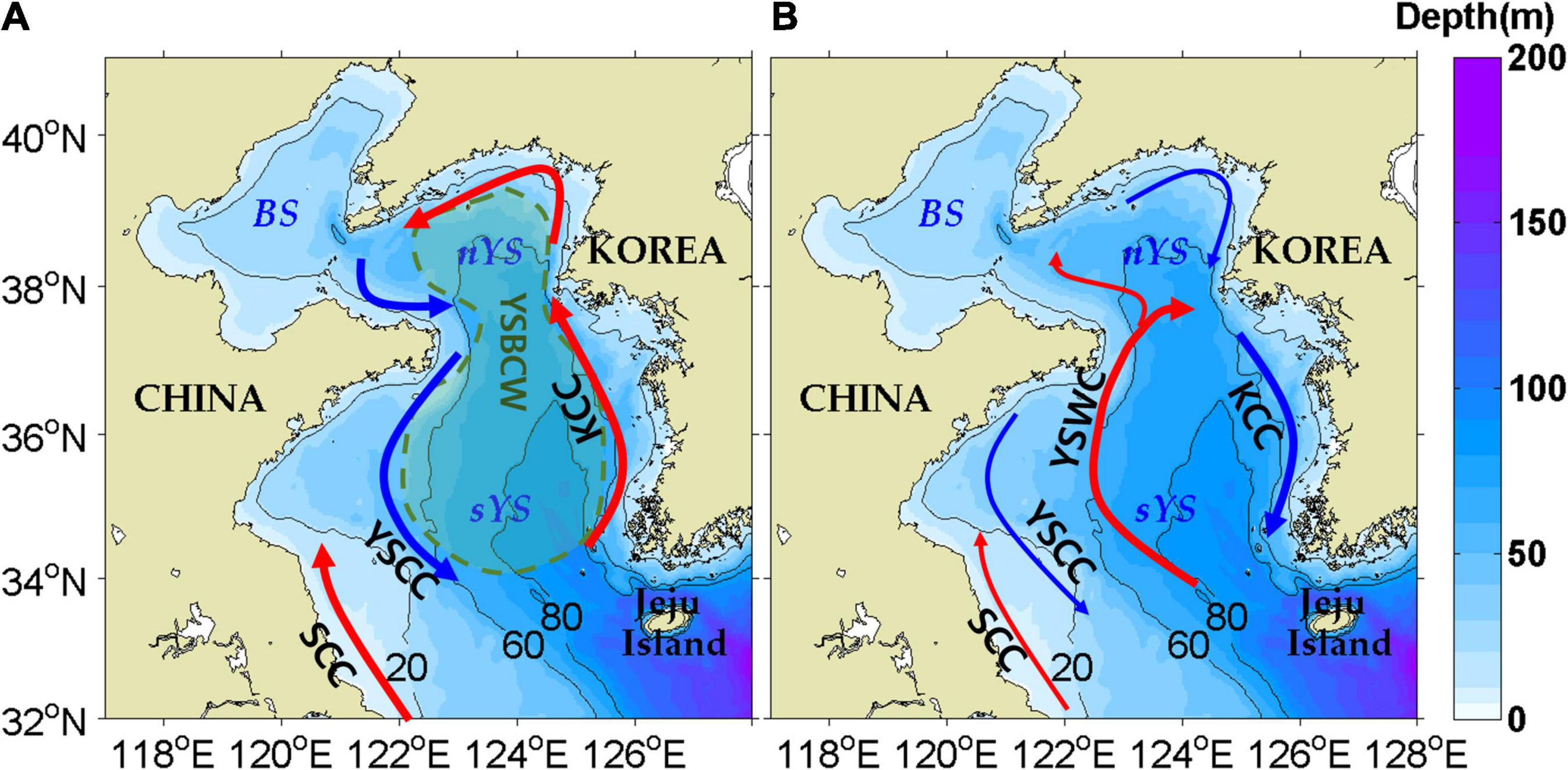
Figure 1. Schematic diagrams of ocean currents during summer (A) and winter (B) in the Yellow Sea. KCC, SCC, YSCC, YSBCW, YSWC, BS, nYS, and sYS indicate the Korean Coastal Current, Subei Coastal Current, Yellow Sea Coastal Current, Yellow Sea Bottom Cold Water, Yellow Sea Warm Current, Bohai Sea, northern Yellow Sea, and southern Yellow Sea, respectively.

important species of fixed nitrogen for primary production and aquaculture in the YS (Fu et al., 2009; Jin et al., 2013; Liu et al., 2017).

Seaweed aquaculture is an important industry in the coastal area of the YS during winter (Chengkui, 1984; Kim et al., 2017; Park et al., 2018). The chlorosis presumably caused by NO₃^– depletion has frequently damaged the aquaculture industry along the Korean coast since 2010 (NFRDI, 2014; Shim et al., 2014). At the same time, eutrophication has caused significant algal blooms along the coast of China, having negative impacts on fishery resources (Liu et al., 2013; Li et al., 2015).

Several studies have investigated NO₃^– flux in the YS using a range of methods (Liu et al., 2003; Wu et al., 2019; Guo et al., 2020). Liu et al. (2003) quantified nutrient fluxes using a single box model but did not consider the effect of currents and in situ biological processes (e.g., nitrification and NO₃^– uptake by phytoplankton). Wu et al. (2019) reported the importance of nitrification for NO₃^– flux in the YS using isotope analysis without quantitative assessment. Guo et al. (2020) showed the effects of physical and biological processes in the southern YS focusing on three different regions. Riverine input, atmospheric deposition, anthropogenic input, and flux from sediments have been suggested as NO₃^– sources in the YS (Bashkin et al., 2002; Lim et al., 2008; Li et al., 2015). However, the effect of advection by currents has not yet been quantitatively assessed.

Circulation in the YS is dominated by the East Asian Monsoon system. In summer, cyclonic circulation occurs due to the baroclinic effect of strong solar radiation and river inputs to the YS, and the northward Subei Coastal Current (SCC) occurs along the Chinese coast (Figure 1A; Yanagi and Takahashi, 1993; Hwang et al., 2014; Yuan et al., 2017; Wu et al., 2018; Xing et al., 2020). In winter, the Yellow Sea Warm Current (YSWC) is the dominant flow due to the northwesterly monsoon (Uda, 1934; Hsueh, 1988; Beardsley et al., 1992; Teague and Jacobs, 2000; Lie et al., 2001; Lin et al., 2011; Tak et al., 2016). The northwesterly wind also generates southward downwind flows known as the Korean Coastal Current (KCC) and Yellow Sea Coastal Current (YSCC) (Figure 1B). The northward YSWC turns eastward off the Shandong Peninsula and connects to the southward KCC, resulting in anticyclonic circulation (Yanagi and Takahashi, 1993; Lin and Yang, 2011; Tak et al., 2020).

Transport via these various currents can influence the seasonal distribution of nutrients in the YS. The YSWC reportedly plays an important role in spring bloom by providing external nutrients to the YS (Hyun and Kim, 2003; Fu et al., 2009; Xuan et al., 2011; Jin et al., 2013; Zhou et al., 2013; Liu et al., 2015a,b; Guo et al., 2020). Zhou et al. (2013) reported that wind speed is significantly correlated with the spring bloom by intensifying the nutrient-carrying YSWC in the deep layer. Some sparse observations also implied that the YSWC provides relatively high amounts of nutrients to the phytoplankton community (Jin et al., 2013; Liu et al., 2015a). In addition to the YSWC, the KCC, YSCC, and SCC may also affect nutrient distributions via physical transport.

The Yellow Sea Bottom Cold Water (YSBCW) likely stores the nutrients supplied by organic matter decomposition (Hyun and Kim, 2003; Jang et al., 2013; Wei et al., 2016; Fu et al., 2018; Wu et al., 2019; Guo et al., 2020). Wu et al. (2019) argue that nitrification is the major biological process in the interior of the YSBCW resulting in increased NO₃^– concentration from spring to fall. The accumulated NO₃^– in the YSBCW is supplied to the surface layer through vertical mixing by wind and cooling in winter. In addition, the YSBCW may transport NO₃^– southward from the YS to the East China Sea (ECS) by upwind flow in summer (Yang et al., 2014).

The effects of the currents and biological processes on NO₃^– fluxes are yet to be quantitatively investigated. Moreover, the distinct seasonal differences in the circulation and hydrography in the YS warrant further investigation. Using a three-dimensional (3D) physical-biogeochemical coupled numerical model, this study aimed to quantitatively deconvolute the NO₃^– flux in the YS to advective transport by currents and biological process.

Materials and Methods

Data and Model Configuration

The physical numerical model applied for the study was the Regional Ocean Modeling System (ROMS), a free-surface model with horizontally curvilinear and vertically terrain-following coordinates that solves hydrostatic, incompressible, primitive equations (Shchepetkin and McWilliams, 2005). The model domain ranged zonally from 117.5 to 130.3°E and meridionally from 24.8 to 41.0°N including the ECS and YS (Figure 2A). Bottom topography data were derived from Kim C. -S. et al. (2013). The model grid resolution was approximately 1/30 degrees horizontally and 40 sigma layers vertically.

FIGURE 2

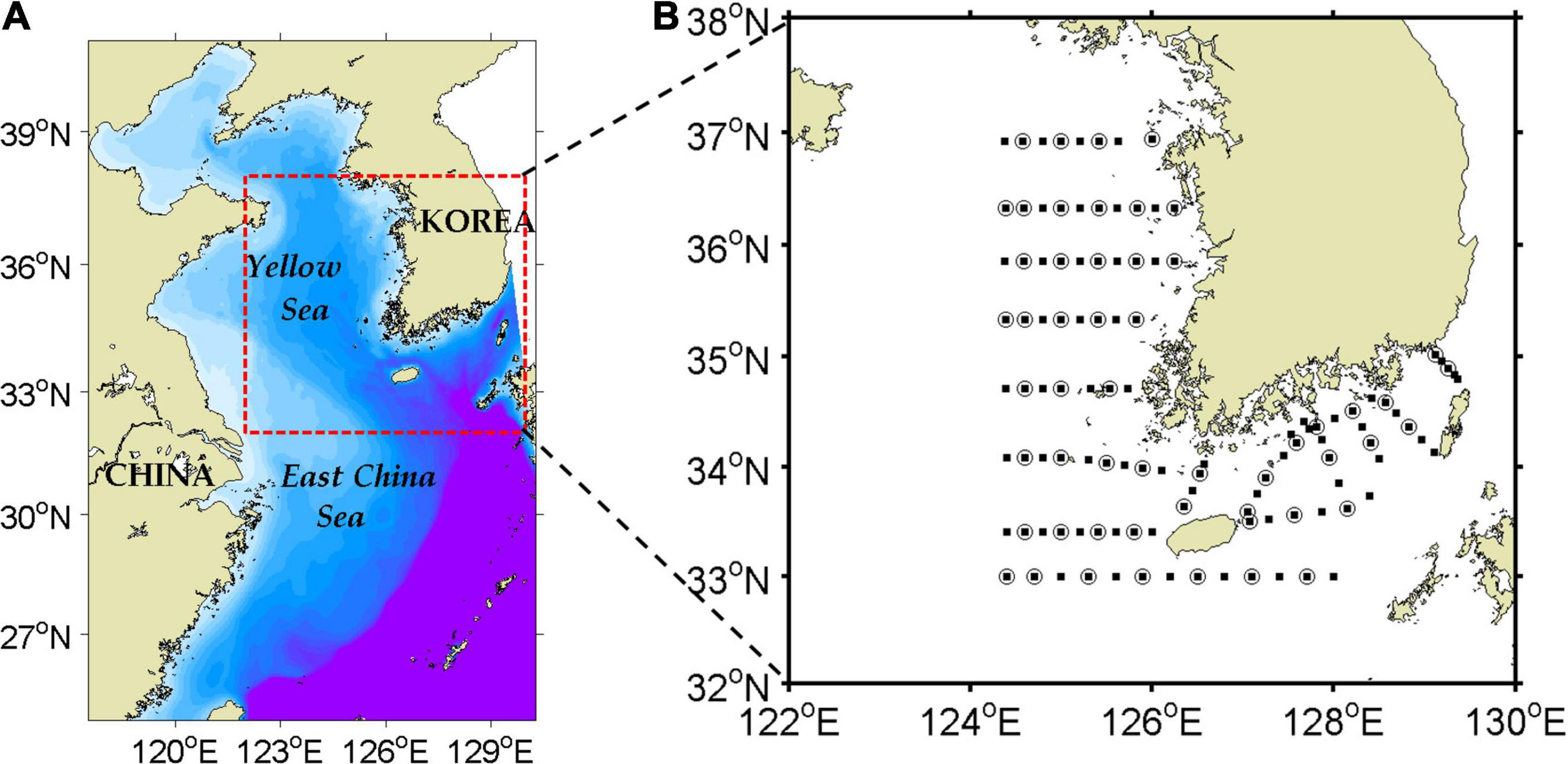
Figure 2. Model domain (A) and routine observation stations (B) taken by the National Institute of Fisheries Science, Korea. Stations for temperature and salinity are denoted by filled squares, and stations for NO₃^– are denoted by open circles. The blue dashed box (zonally from 121.5 to 125.5°E and meridionally from 34.5 to 39.5°N) in (B) denotes the region of the central YS where chlorophyll-a from the model was compared with satellite data for model validation.

The horizontal advection scheme used third-order upstream advection. The horizontal harmonic mixing scheme and the K-Profile parameterization scheme were applied (Large et al., 1994). For the lateral open boundary, monthly mean temperature, salinity, sea surface height, and velocity data were obtained from the Northwestern Pacific Model (Seo et al., 2014). For the surface forcing data, six-hourly wind, air temperature, sea level pressure, relative humidity, daily solar radiation, and precipitation datasets were obtained from the ERA5 reanalysis data of the European Centre for Medium-Range Weather Forecasts (Copernicus Climate Change Service, 2017). The surface heat flux was calculated using bulk formulae (Fairall et al., 1996).

Tidal forcing of 10 tidal components obtained from TPXO6 was imposed at the lateral boundaries of the model (Egbert and Erofeeva, 2002). Monthly mean river discharge was applied for 12 rivers in the BS and YS, freshwater discharge from the Changjiang River was observed at the Datong station, discharge data for Han and Geum Rivers along the eastern coast of the YS were derived from the National Institute of Environmental Research (NIER), and discharge data for all other rivers along the Chinese and Korean coasts were obtained from the Global River Discharge Database (Vörösmarty et al., 1996; Wang et al., 2008). The initial temperature and salinity for an experiment were obtained from the National Ocean Data Center World Ocean Atlas 2013 (WOA2013) (Locarnini et al., 2013; Zweng et al., 2013). The initial velocity field was calculated by the geostrophic equation using the initial temperature and salinity.

Primary production in the YS is not limited by silicate but by nitrogen or phosphorus (Wang et al., 2003; Jin et al., 2013). Thus, a biogeochemical model based on the nitrogen and phosphorus cycles is appropriate for simulating the biogeochemical environment in the YS. The biogeochemical model coupled with the physical model is based on the nitrogen and phosphorus cycles described by Fennel et al. (2006) and Gan et al. (2014). A schematic diagram for the biogeochemical model is shown in Figure 3. The scheme includes the following 10 prognostic variables: phytoplankton, chlorophyll-a, zooplankton, small nitrogen detritus (SDN), small phosphorus detritus (SDP), large nitrogen detritus (LDN), large phosphorus detritus (LDP), NO₃^–, NH₄⁺, and phosphate (PO₄^3–).

FIGURE 3

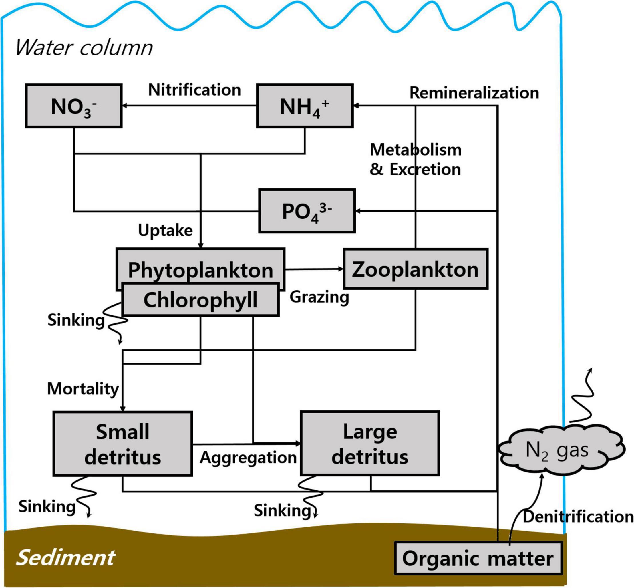
Figure 3. A biogeochemical model schematic for the nitrogen and phosphorus cycles based on Fennel et al. (2006) and Gan et al. (2014).

The growth of phytoplankton depends on temperature, radiation, and nutrient concentrations, and radiation is attenuated by water and chlorophyll-a concentrations. The attenuation coefficient by water (K_w) was set to 0.09 m⁻¹ in the entire model domain, which is higher than the model default value (0.04 m⁻¹) because the turbidity in the YS is considerably high (Shi and Wang, 2012). According to prior studies, the light attenuation coefficient (K_d), which is calculated by the sum of the K_w and multiplying the light attenuation coefficient for chlorophyll-a (K_chl) by the integration of chlorophyll-a in the water column in the biogeochemical model, can be estimated by an empirical equation as follows (Holmes, 1970; Castillo-Ramírez et al., 2020):

$K_d=1.4/Z_{SD},(1)$

where Z_SD denotes the Secchi disk depth. In situ observation by the National Institute of Fisheries Science (NIFS), Korea, showed that the annual mean Z_SD was 10 m at the central stations and 5 m at the coastal stations in the YS. Thus, K_d in the central and coastal stations can be estimated as 0.14 and 0.28 m⁻¹, respectively. However, because the Secchi disk depth includes an attenuating effect of phytoplankton and the model domain is based on open ocean, we performed several sensitivity tests for evaluating a reasonable attenuation coefficient and selected 0.09 m⁻¹ as an adequate value in the YS.

Uptakes of NO₃^–, NH₄⁺, and PO₄^3– are estimated by Michaelis–Menten equations with preferential consumption of NH₄⁺ in the nitrogen uptake by phytoplankton (Menten and Michaelis, 1913). The model assumed that organic matter decomposition was converted to inorganic nutrients as soon as the organic matter reached the bottom layer because approximately 90% of the organic matter derived from primary production is mineralized in the water column (Song et al., 2016). In other words, sediment nutrient flux into the bottom layer was employed without a time lag because only 10% of the organic matter could reach the sediment. Since most of the organic matter should be remineralized before reaching the bottom layer in the YS, the small and large detritus remineralization rates were set to 0.04 and 0.02 d⁻¹, respectively. Fennel et al. (2006) estimated that 14% of organic matter decomposition involved denitrification in the Mid-Atlantic Bight region. However, we assumed that 9% of the decomposition was denitrified because the YS maintained a sufficient level of oxygen to suppress denitrification and the organic matter content in the surface sediment was low, indicating that biological processes in the sediment may play a secondary role in the YS (Zhao et al., 2018; Wu et al., 2019).

The velocities of large detritus, small detritus, and phytoplankton were set to 2.0, 0.2, and 0.1 md⁻¹, respectively, which were within the range of general sinking velocities in the ocean based on observation, the Stokes equation, and sensitivity model analyses considering the size and density of a particle (Smayda, 1969; Fasham et al., 1990; Moskilde, 1996). In addition to particle characteristics, sinking velocity can also be regulated by seawater density. Thus, the empirical equation for vertical sinking velocities of phytoplankton and detritus was modified depending on temperature (as the main control of the seawater density) as per Bach et al. (2012). Accordingly, the sinking velocity doubled as the temperature increased by 15°C at a salinity of 35 gkg⁻¹. Considering the salinity variation from 29 to 34 gkg⁻¹ in the YS, the velocity equation in the model was modified to increase with temperature more rapidly as follows:

$\{\begin{array}{c}\hfill W_p=\frac{W_d}{3}(T<{\mathrm{\hspace{0.25em}10}}^{°}C)\hfill \\ \hfill W_p=\frac{W_d}{\left\{3-2\left(\frac{\mathrm{T}-10}{15}\right)\right\}}(10\le T\le {25}^{°}C)\hfill \\ \hfill W_p=W_d(T>{25}^{°}C)\hfill \end{array}(2)$

where T is temperature, and W_p and W_d are the particle sinking velocity under the temperature-varying condition and the default value of the velocity, respectively.

Several biological parameters related to primary production, such as the initial slope of the photosynthesis-irradiance curve, maximum chlorophyll to phytoplankton ratio, half-saturation for phytoplankton of NH₄⁺ uptake, phytoplankton and zooplankton mortality rates, zooplankton grazing rate, and zooplankton half-saturation constant for ingestion, were tuned properly for the YS environment to simulate the spring bloom and its magnitude. Further details on the nitrogen and phosphorus cycles in the biogeochemical model are described in Fennel et al. (2006) and Gan et al. (2014). The biogeochemical parameters applied in the model are provided in Table 1.

TABLE 1

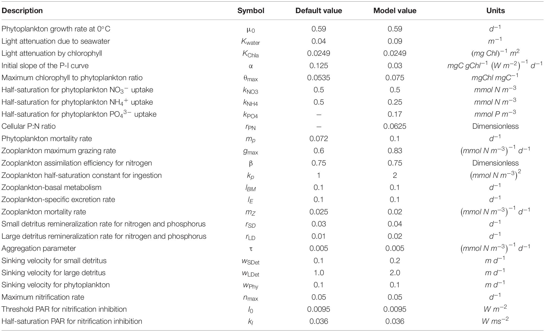
Table 1. Biogeochemical model parameters used in this study and default values from Fennel et al. (2006).

The initial and boundary conditions for chlorophyll-a in the water column were based on climatological monthly mean surface chlorophyll-a data obtained from the Moderate Resolution Imaging Spectroradiometer (MODIS)-aqua and an empirical model (Morel and Berthon, 1989; Uitz et al., 2006). The initial and boundary concentrations of NO₃^– and PO₄^3– were derived from the WOA 2013 dataset, and the concentration of NH₄⁺ was set to 1 μmolL⁻¹ as described by Garcia et al. (2013). The initial conditions of phytoplankton, zooplankton, and large and small detritus were estimated from the phytoplankton/chlorophyll-a, zooplankton/chlorophyll-a, and detritus/phytoplankton ratios of 0.5, 0.2, and 0.35, respectively (Gruber et al., 2006). The climatological annual mean concentrations of dissolved inorganic nitrogen and phosphorus in the 2000s, and the NO₃^–/ NH₄⁺ ratio for the Changjiang River, were applied in the model (Dai et al., 2011; Wang et al., 2011; Zhou et al., 2017). For the Yellow River, the annual mean concentrations of NO₃^–, NH₄⁺, and PO₄^3– for the period 2002–2004 were derived from Gong et al. (2015), and the respective concentrations in the Yalu River were obtained from Liu and Zhang (2004) for 1992, 1994, and 1996. The monthly mean riverine NO₃^–, NH₄⁺, and PO₄^3– inputs from the Korean Peninsula were obtained from the NIER. Constant atmospheric depositions of NO₃^–, NH₄⁺, and PO₄^3– of 0.027 mmolNm⁻²d⁻¹, 0.080 mmolNm⁻²d⁻¹, and 0.001 mmolPm⁻²d⁻¹, respectively, were applied to the surface boundary conditions based on previous observations (Zhang, 1994; Li et al., 2015).

The coupled model was spun up for 7 years and was integrated for the period 2006–2019. To evaluate the performance of the model, the simulated temperatures, salinities, and NO₃^– concentrations in the YS were compared to bimonthly observational data obtained from the NIFS, Korea, for the corresponding period (Figure 2B). Data that deviated from the mean by more than one standard deviation were excluded from the analysis.

Estimation of Nitrate Flux

The temporal variation in NO₃^– concentrations is expressed as follows:

${\displaystyle \frac{\partial \left[N{O}_3^{-}\right]}{\partial t}}=\left(-\overrightarrow{u}\cdot \nabla \left[N{O}_3^{-}\right]\right)+\left(k_T{\nabla }^2\left[N{O}_3^{-}\right]\right)+\left(-U_{NO3}\cdot \left[Phyto\right]\right)+\left(L_{nitri}\cdot \left[N{H}_4^{+}\right]\right),(3)$

where $\left[N{O}_3^{-}\right],\left[N{H}_4^{+}\right],\left[Phyto\right],\overrightarrow{u},k_T,U_{NO3},\mathrm{and}{L}_{nitri}$ are the NO₃^–, NH₄⁺, and phytoplankton concentrations, three-dimensional velocity, diffusion, uptake rate of NO₃^–, and nitrification rate, respectively. The terms on the right side of the equation indicate advection, diffusion, NO₃^– uptake by phytoplankton, and nitrification, respectively. The first two terms are controlled by physical processes while the remaining terms are controlled by biological processes. The diffusion term was ignored in this study because it is almost negligible compared with the advection term. The effect of currents on NO₃^– flux is reflected by the advection term. The uptake rate is defined as follows:

$U_{NO3}={\mathrm{\mu }}_{max}f\left(I\right)L_{NO3,}(4)$

where μ_max,f(I),andL_NO3 are the maximum growth rate, photosynthesis-light relationship, and half-saturation concentration for the uptake of NO₃^–, respectively. The maximum growth rate and photosynthesis-light relationship are defined as follows:

${\mathrm{\mu }}_{max}={\mathrm{\mu }}_0\cdot {1.066}^T,(5)$

$f\left(I\right)=\frac{\mathrm{\alpha }I}{\sqrt{\mathrm{\mu }_{max}{}^2+{\mathrm{\alpha }}^2{I}^2}},(6)$

where μ₀,T,I, and α are the phytoplankton growth rate at 0°C, temperature, photosynthetically active radiation, and initial slope, respectively. I decreases exponentially with depth in the water column (z), where:

$I(z)=I_s\cdot PARfrac\cdot exp\left\{-z\left(K_w+K_{chl}{\int }_z^{0}Chl\left(\mathrm{\zeta }\right)\mathit{d}\mathrm{\zeta }\right)\right\},(7)$

where I_s,PARfrac,K_chl,andChl(ζ) are the shortwave radiation flux, fraction of light, light attenuation coefficient for chlorophyll-a, and chlorophyll-a concentration at a depth of ζ m, respectively. L_nitri is calculated as follows:

$L_{nitri}=n_{max}\left(1-max[0,\frac{I-I_0}{k_I+I-I_0}]\right),(8)$

where n_max, k_I, and I₀ are the maximum rate of nitrification, half-saturation for light inhibition, and inhibition threshold, respectively.

Model Validation

To validate model performance, simulated temperatures, salinities, and NO₃^– concentrations were compared with observational data in February and August. For comparison, climatological mean data were produced from bi-monthly observation data in the southeastern YS region for the period 2006–2019. Figures 4–6 show horizontal distributions of temperature, salinity, and NO₃^–, respectively, for the climatological observations and model results at the surface and at a depth of 50 m in February and August.

FIGURE 4

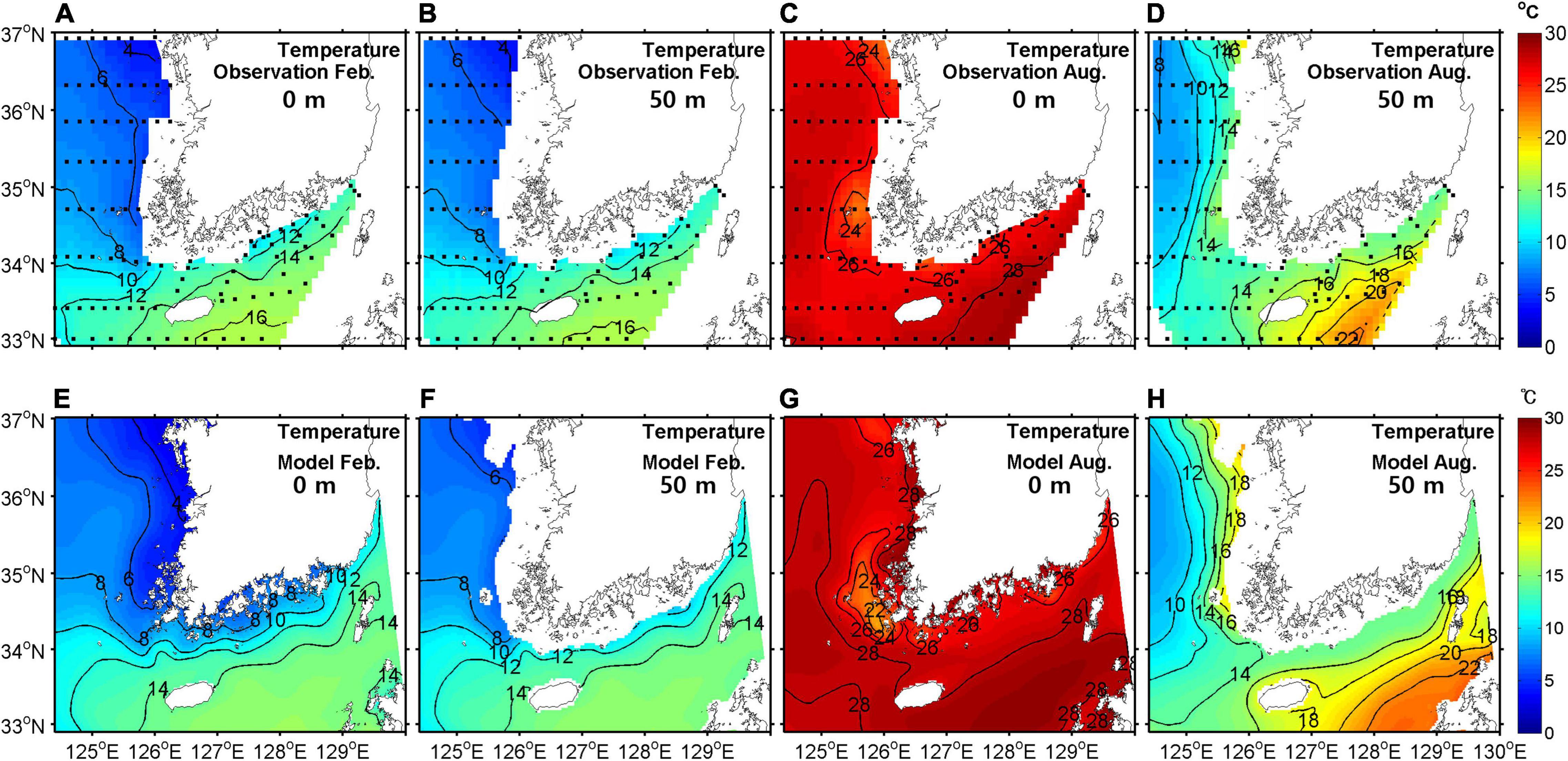
Figure 4. Horizontal distribution of temperature from observations (upper) and model outputs (lower) at the surface (A,C,E,G) and at a depth of 50 m (B,D,F,H) in February (A,B,E,F) and August (C,D,G,H) averaged for the period 2006–2019 (units are °C).

FIGURE 5

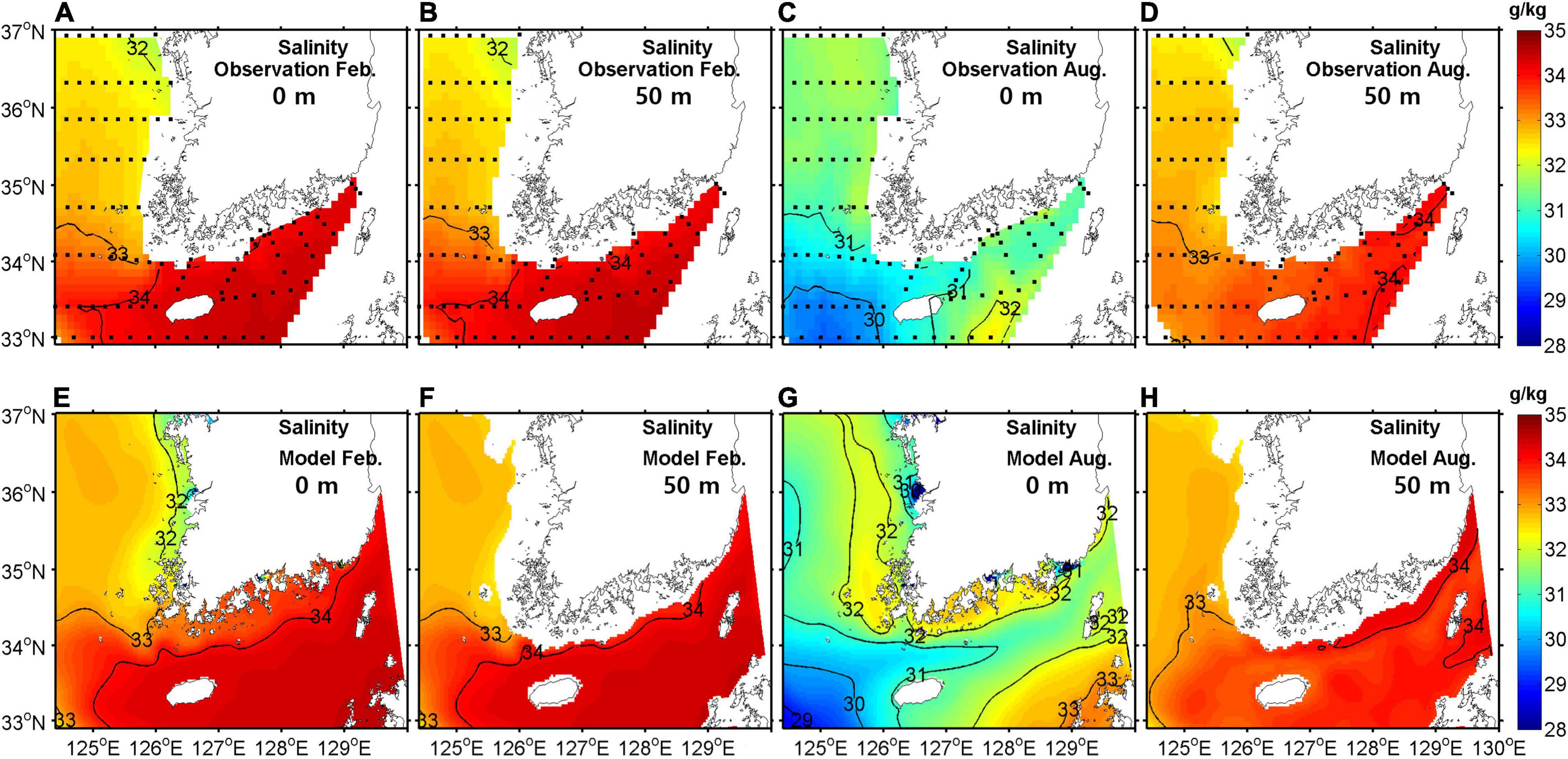
Figure 5. Horizontal distribution of salinity from observations (upper) and model outputs (lower) at the surface (A,C,E,G) and at a depth of 50 m (B,D,F,H) in February (A,B,E,F) and August (C,D,G,H) averaged for the period 2006–2019 (units are gkg⁻¹).

FIGURE 6

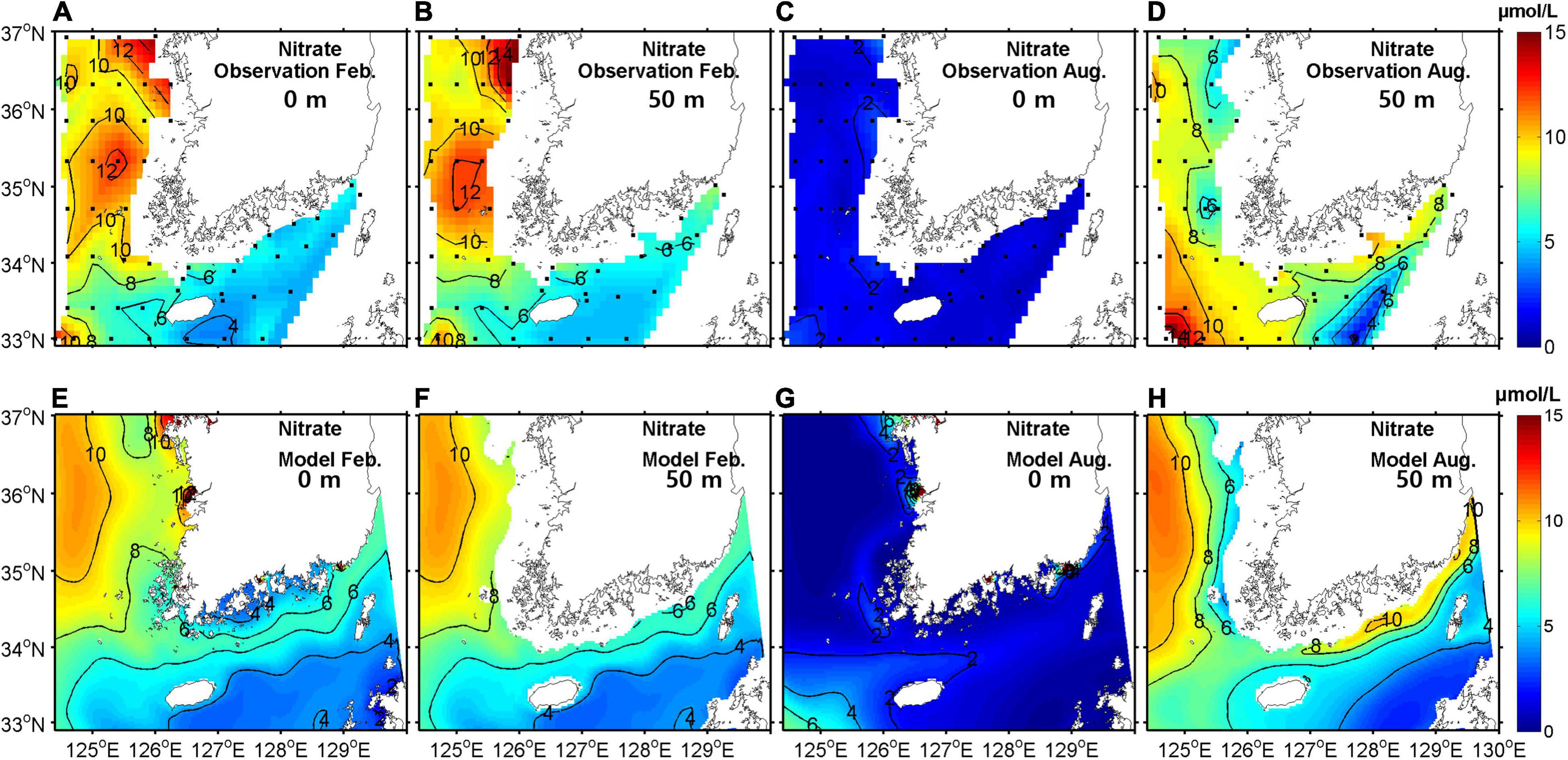
Figure 6. Horizontal distribution of NO₃^– concentrations from observations (upper) and model outputs (lower) at the surface (A,C,E,G) and at a depth of 50 m (B,D,F,H) in February (A,B,E,F) and August (C,D,G,H) averaged for the period 2006–2019 (units are μmolL⁻¹).

In February, the horizontal distribution at the surface showed the same pattern as at a depth of 50 m due to strong vertical mixing. A warm, saline, and low NO₃^– tongue was present in the eastern entrance of the YS, which was properly represented by the model. The concentration of NO₃^– was high in the eastern YS.

In August, the surface temperature was mostly higher than 26°C and relatively low along the western coast of the Korean Peninsula due to tidal mixing (Sun and Cho, 2010). The YSBCW was colder than 10°C in the central YS at 50-m depth. A low salinity patch (<31 gkg⁻¹) appeared near Jeju Island, particularly in the western region of the island because of dilution by water from the Changjiang River. The surface NO₃^– concentration was low due to primary production but high in the western region of Jeju Island with lower-salinity waters, which was somewhat overestimated in the model. At a depth of 50 m, the NO₃^– concentration was high but relatively low in the Kuroshio Current waters, which lay east of Jeju Island. Overall, the seasonal patterns of temperature, salinity, and NO₃^– were well simulated in the coupled model.

The seasonal distributions of simulated DIN concentration were also compared in the western and central YS with the distributions presented in Wei et al. (2016; Supplementary Figure 1). We estimated DIN as the sum of NO₃^– and NH₄⁺ and compared it with the observed DIN distributions. Surface DIN concentration is high in the central YS in winter. It decreases in summer except for high values in the mouth of the Changjiang River. The concentration increases in fall again. At the bottom layer, the DIN concentration is minimal in spring due to bloom and maximal in fall due to remineralization. The DIN concentration is normally high in the central YS where the YSBCW is located.

Due to massive fishery activities and extreme weather conditions in the YS, it is difficult to obtain long-term current data by moorings. Instead of current, surface temperatures obtained from the Advanced Very High Resolution Radiometer (AVHRR) satellite data were compared with those from model results averaged from 2006 to 2019, because horizontal distributions of surface temperature mainly depend on currents. The spring, summer, fall, and winter seasons were defined as March to May, June to August, September to November, and December to February, respectively. The distributions from the model results presented an intrusion of warm water by the YSWC during winter and a tidal front along the Korean coast during summer and fall, indicating that the advection and mixing by currents in the YS were simulated properly with the satellite data (Figure 7).

FIGURE 7

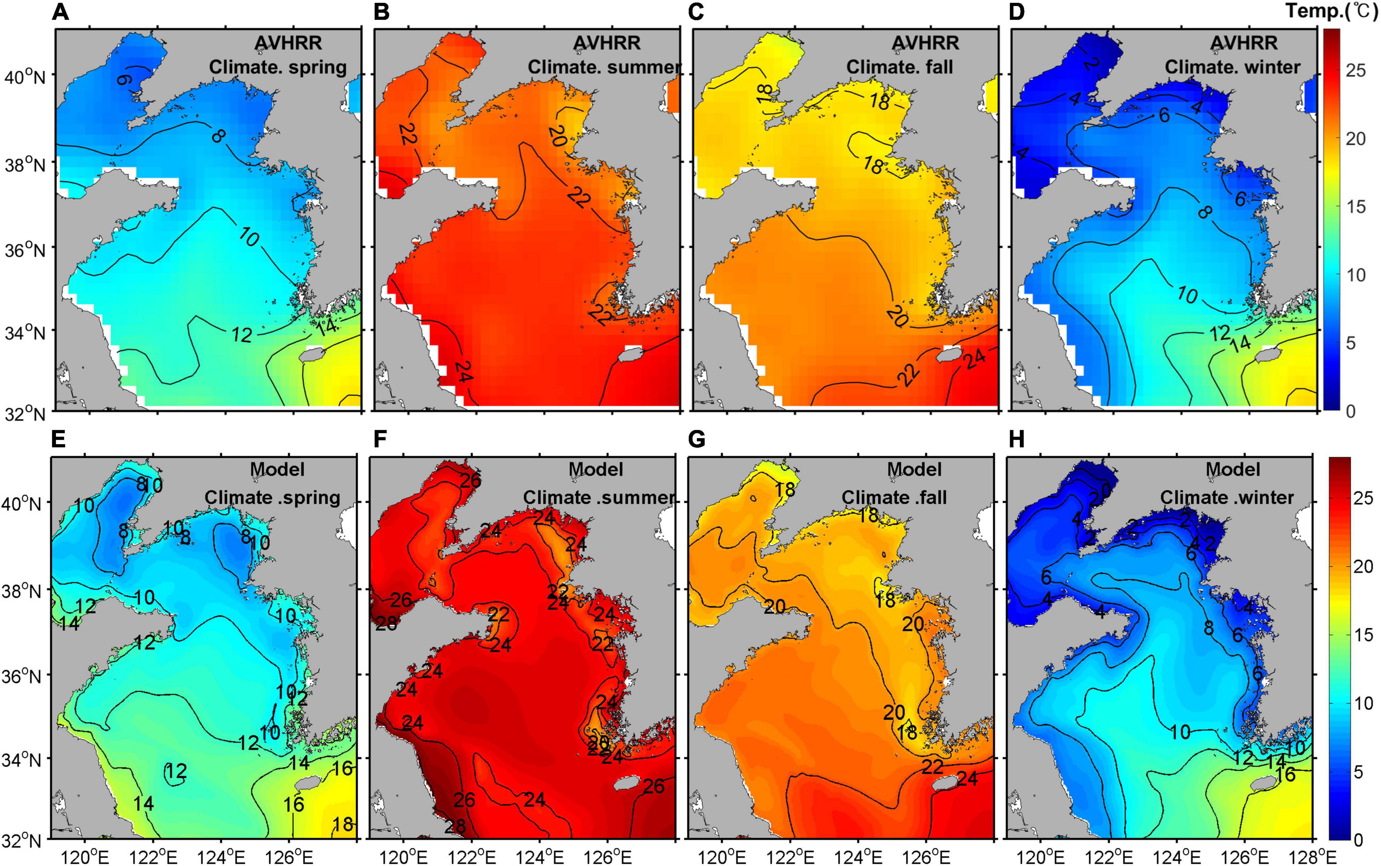
Figure 7. Horizontal distribution of surface temperature from the AVHRR satellite data (A–D) and model outputs (E–H) in spring (A,E), summer (B,F), fall (C,G), and winter (D,H) averaged for the period 2006–2019 (units are °C). AVHRR, Advanced Very High Resolution Radiometer.

For the comparison of chlorophyll- a distributions, only the data in the central region of the YS (121.5–125.5°E, 34.5–39.5°N) were selected because the chlorophyll-a concentration derived from satellite data was highly overestimated due to the resuspension of sediments in the coastal region of the YS and Bohai Sea (BS) (Yamaguchi et al., 2012; Shi et al., 2017). The model results were compared with the spatially averaged chlorophyll-a concentrations derived from MODIS-aqua for the corresponding period (Figure 8). Tan and Shi (2012) reported spring and fall blooms based on seasonal primary production patterns in the YS. Chlorophyll-a concentrations observed by satellite in winter were higher than those in fall. The high chlorophyll-a in winter from the satellite data might result from particle resuspension by active vertical mixing driven by strong winds in winter (Kiyomoto et al., 2001; Siswanto et al., 2011; Yamaguchi et al., 2012). Low planktonic biomass from in situ observations in winter supports this interpretation (Fu et al., 2009; Siswanto et al., 2011).

FIGURE 8

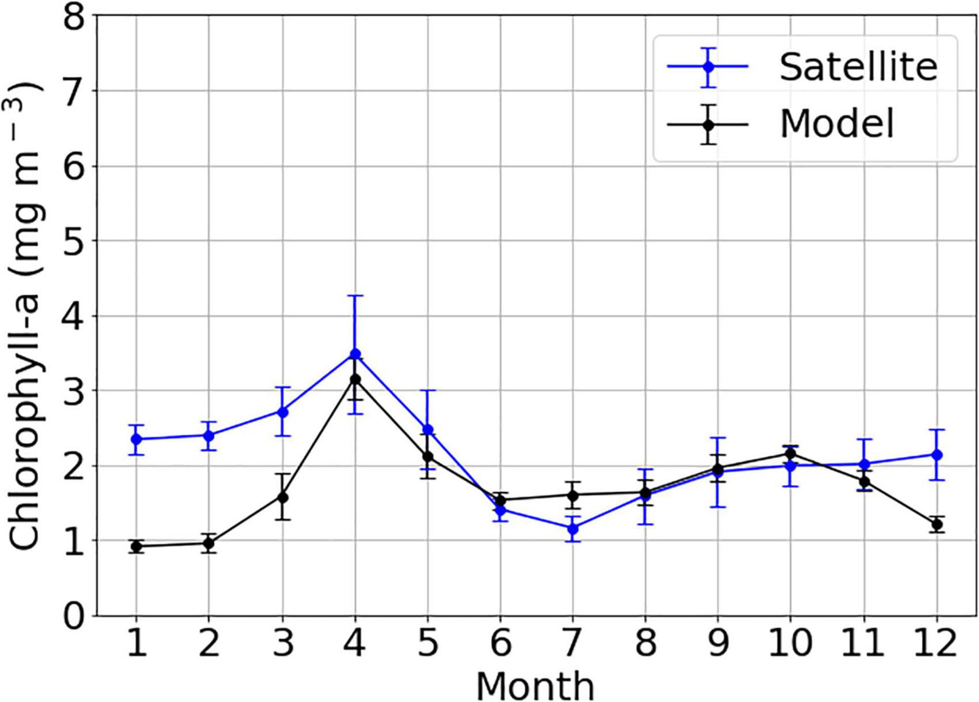
Figure 8. Time-series of climatological monthly mean of chlorophyll-a concentrations from satellite data (blue line) and model outputs (black line) averaged over the central YS (121.5–125.5°E, 34.5–39.5°N) from 2006 to 2019 (units are mg m⁻³). Vertical bars indicate the standard deviation of interannual variation. YS, Yellow Sea.

Overall, the Taylor diagram in Figure 9 objectively presents the model performance for temperature, salinity, NO₃^–, and chlorophyll-a. The abnormal chlorophyll-a concentration in winter derived from the satellite data was excluded when estimating correlation, root mean square, and standard deviation. All variables except for those at a 50-m depth were close to the observation point denoted by a black star in the x-axis and had strong correlations higher than 0.7, suggesting that the model results nearly corresponded to the observations. The correlation coefficients and normalized standard deviations for salinity and NO₃^– at a depth of 50 m were relatively lower than other variables but the p-values for those variables were below 0.05, indicating significant correlations. Using various analyses of the coupled model and observation data, simulated seasonal cycles of temperature, salinity, NO₃^–, and chlorophyll-a by the coupled model were quantitatively evaluated and were consistent with the observations.

FIGURE 9

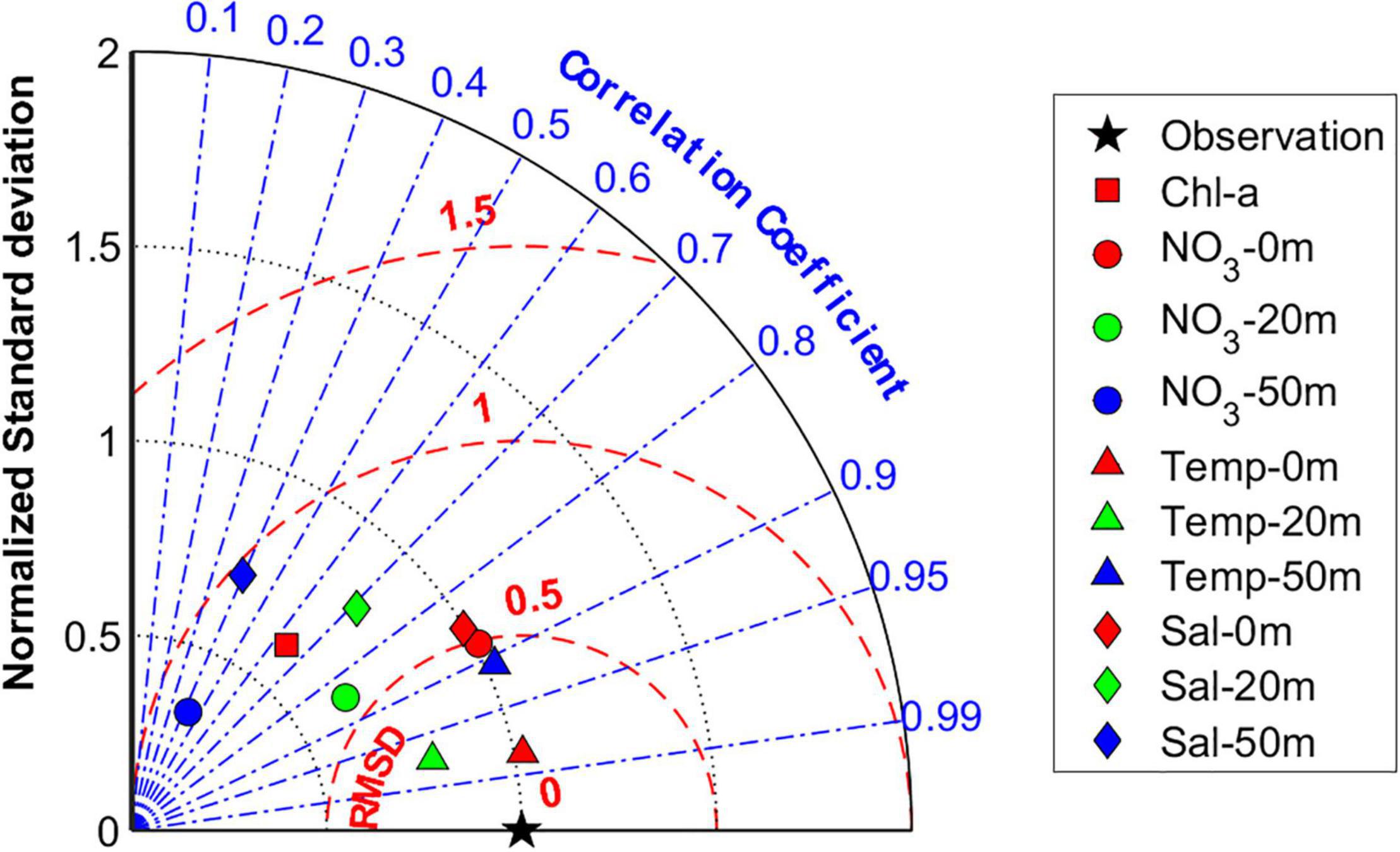
Figure 9. Normalized Taylor diagram comparing simulated monthly mean chlorophyll-a concentration (squares), spatially averaged in the central YS (121.5–125.5°E, 34.5–39.5°N), NO₃^– concentration (circles), temperature (triangles), salinity (diamonds) at the surface (red) and depths of 20 m (green) and 50 m (blue) averaged at stations denoted in Figure 2B with satellite, NIFS observation data (the reference field denoted by black star on the x-axis). The radial coordinate is the magnitude of normalized standard deviation from observation. The concentric red semi-circles indicate Root Mean Square Difference (RMSD). The angular coordinate shows the correlation coefficient (denoted by blue dotted lines). YS, Yellow Sea; NIFS, National Institute of Fisheries Science.

Results and Discussion

Subdivision of the Yellow Sea Based on Nitrate Flux Along the Southern Boundary and the Dominant Currents

Vertical sections of NO₃^– concentrations, meridional velocity, and NO₃^– flux along the southern boundary (34.5°N) of the YS in January and July are shown in Figure 10. In winter, the main advective NO₃^– influxes resulted from the YSWC in the trough of the YS and SCC along the Chinese coast (Figure 10E). Advective outfluxes occurred with the KCC along the Korean coast and the southward surface current in the trough region (Tak et al., 2016). The YSCC located between the YSWC and the SCC also contributed to the NO₃^– outflux, although its overall contribution was relatively small (Hwang et al., 2014). In summer, influx of NO₃^– into the YS occurred along the Chinese coast via the SCC and via a northward current on the eastern side of the trough in the subsurface layer (Figure 10F). The outflux of NO₃^– was mainly driven by the southward movement of the YSBCW in the subsurface layer of the trough (Yang et al., 2014).

FIGURE 10

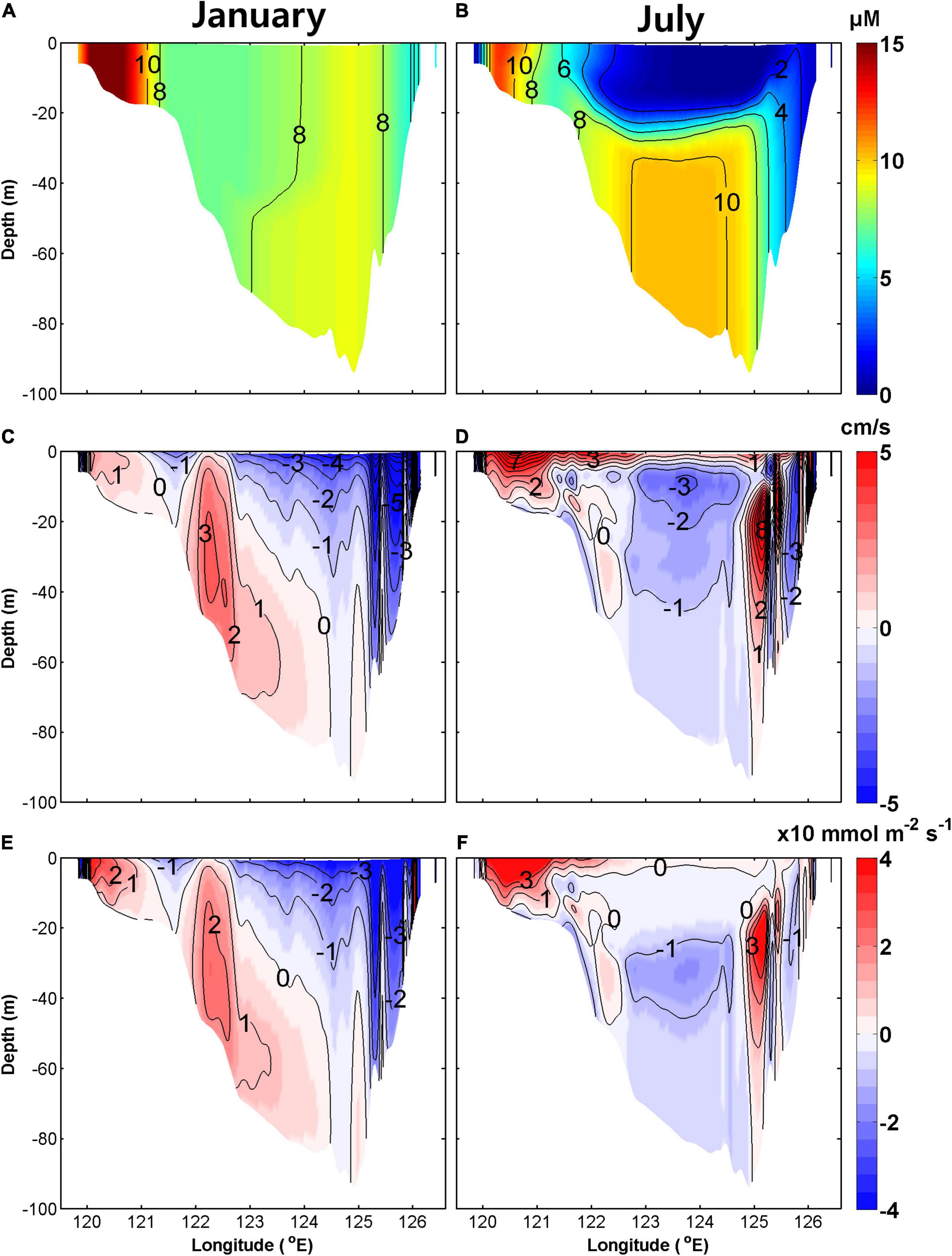
Figure 10. Climatological monthly mean vertical sections of NO₃^– concentration (upper), meridional velocity (middle), and NO₃^– flux (lower) along the 34.5°N section in January (A,C,E) and July (B,D,F) averaged for the period 2006–2019. Colors in upper panels indicate NO₃^– concentrations (μ mol L^–1). Red and blue in middle and lower panels indicate northward and southward velocities (cm/s) and NO₃ fluxes (× 10 mmol m^–2s^–1), respectively.

The southern boundary section can be divided into three areas based on the features of NO₃^– flux. In the western area of the section (119.5–121.6°E), NO₃^– was transported into the YS via the SCC all year. In the central area of the section (121.6–125.2°E), the influx occurred via the YSWC in winter and the outflux occurred via the southward movement of the YSBCW in summer. In the eastern area of the section (125.2–126.5°E), the outflux occurred via the KCC in winter.

Figure 11 shows seasonal mean horizontal velocity distributions at the surface and in the subsurface layers. Considering the surface Ekman layer depth, the surface and subsurface layers were averaged from the surface to a depth of 30 m and from 30 m to the bottom, respectively. The horizontal velocity distributions showed two representative circulation patterns, namely spring-winter and summer-fall patterns (Yanagi and Takahashi, 1993; Hwang et al., 2014). In summer and fall, a strong cyclonic circulation appeared on the surface layer with a southward current in the central YS. In spring and winter, a southward current occurred at the surface layer in the central and eastern YS due to the strong northwesterly winter monsoon, and the northward YSWC occurred in the central YS in the subsurface layer. Anticyclonic circulation appeared in the subsurface layer. In the BS, anticyclonic circulation persisted for all seasons but was weaker than in the YS. The complex system of circulation suggests that the YS should be subdivided to adequately assess the seasonal and spatial variations in NO₃^– flux.

FIGURE 11

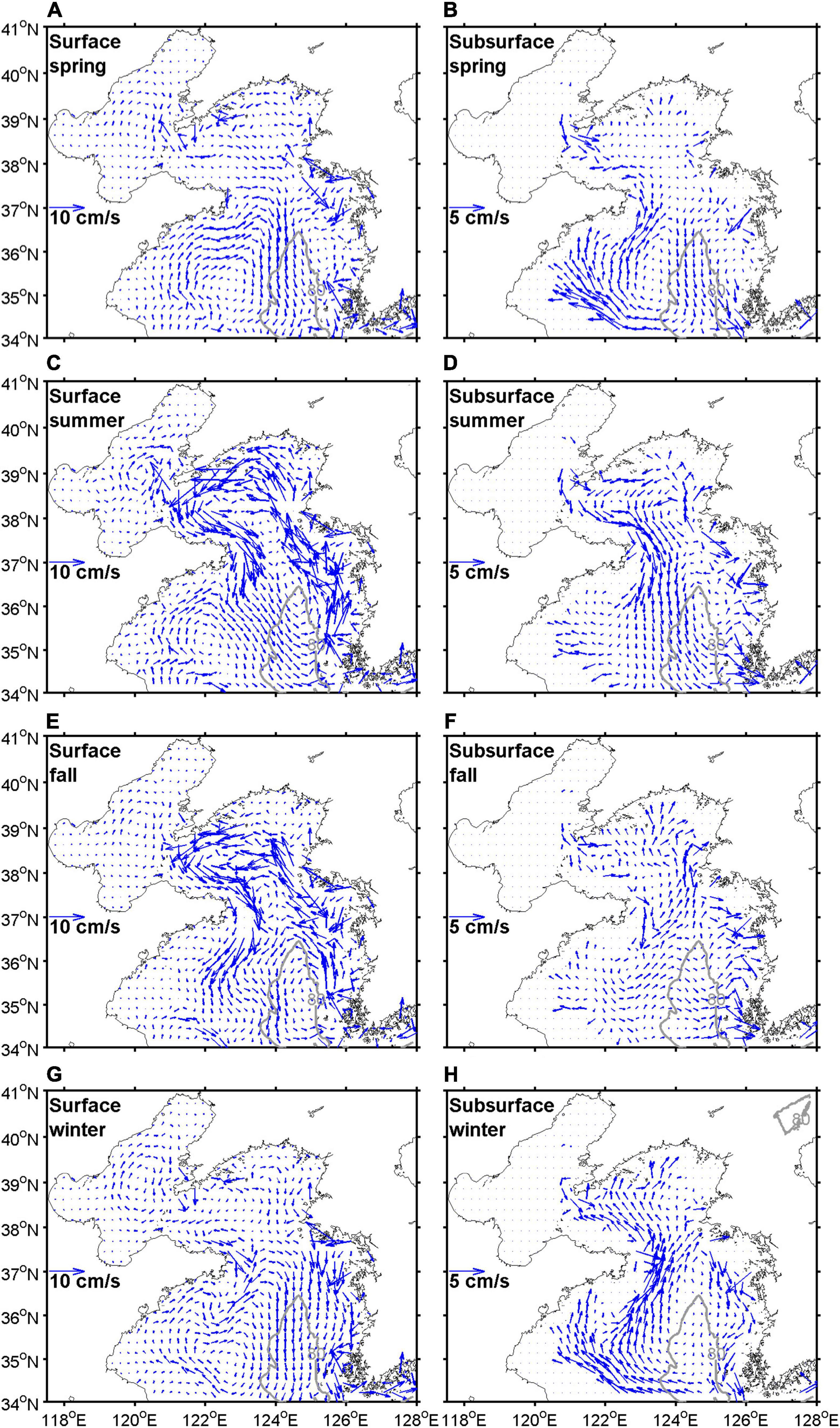
Figure 11. Horizontal velocity distributions at the surface (A–D) and subsurface (E–H) layers during spring (A,E), summer (B,F), fall (C,G), and winter (D,H) averaged for the period 2006–2019. The surface and subsurface layers are averaged from the surface to 30 m depth and from 30 m depth to the bottom, respectively.

Considering these currents, we subdivided the YS into the northern YS (nYS), southeastern YS (seYS), southcentral YS (scYS), and southwestern YS (swYS) as shown in Figure 12A. The BS was designated as a separate subregion. We further divided the boundaries between swYS and scYS, and between scYS and seYS, into northern (solid line) and southern (dashed line) boundaries. The boundary between nYS and scYS was divided into eastern (solid line) and western (dashed line) boundaries.

FIGURE 12

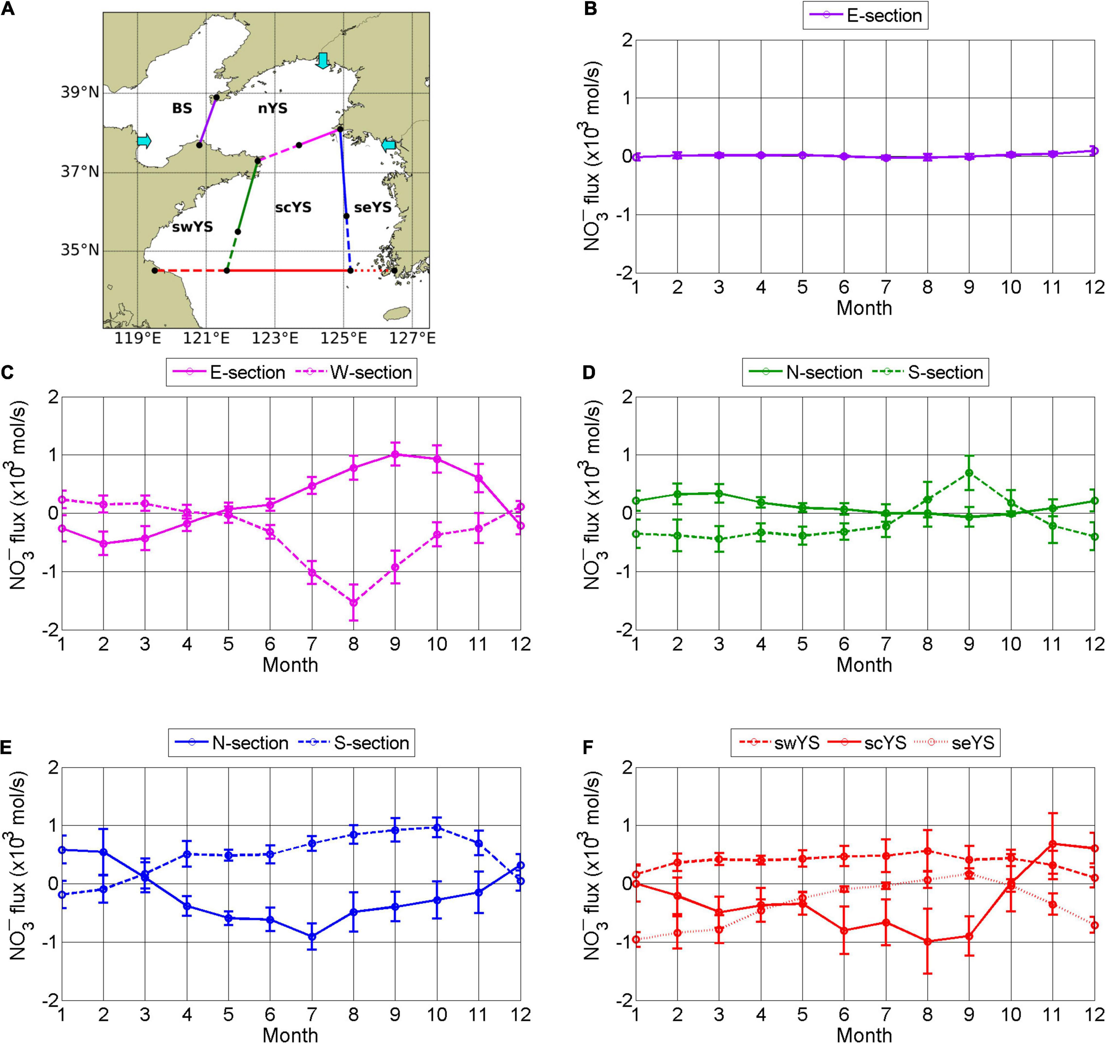
Figure 12. Subregions (A) to estimate NO₃^– flux based on circulation in the YS. BS, nYS, swYS, scYS, and seYS denote the Bohai Sea and the northern, southwestern, southcentral, and southeastern YS, respectively. Cyan arrows indicate NO₃^– flux by rivers from the Korean coast in the seYS, the Yalu River in the nYS, and the Yellow River in the BS. Monthly mean net advective NO₃^– flux between subregions was averaged for the period 2006–2019. The purple (B), magenta (C), green (D), blue (E), and red (F) lines represent boundaries indicated in (A) (kmols⁻¹), where positive values denote eastward and northward fluxes, and negative values denote westward and southward fluxes. YS, Yellow Sea.

Advective Nitrate Flux Across Subregion Boundaries

The monthly mean net advective NO₃^– fluxes by currents among subregions were calculated. The BS supplied NO₃^– to the nYS year round except in summer (Figure 12B). The net advective fluxes across boundaries in the YS exhibited strong seasonal variation. In winter, northward and southward fluxes occurred across the western and eastern boundaries between the nYS and scYS, respectively (Figure 12C). Net fluxes across the meridional boundaries dividing the swYS, scYS, and seYS similarly showed westward and eastward fluxes across the southern and northern boundaries, respectively (Figures 12D,E). Net fluxes in summer occurred in the opposite directions to those in winter in accordance with the circulation direction.

The net advective fluxes across the southern boundary of the YS represent fluxes between the YS and the ECS (Figure 12F). Influx to the swYS (red dashed line) via the SCC along the Chinese coast played a major role in the net influx from the ECS. The net influx to the scYS (red solid line) via the YSWC during winter was relatively small. The mean influx of NO₃^– via the YSWC was 1.4 10³mols⁻¹ during winter but was almost offset by the southward current in the surface layer. Net outfluxes to the ECS occurred from the scYS in summer due to the southward movement of the YSBCW and from the seYS in winter via the KCC along the Korean coast (red dotted line in Figure 12A).

Nitrate Budgets in the Subregions

Monthly mean changes in NO₃^– concentration driven by current advection, biological processes, and riverine input were calculated for each subregion (Figure 13) and are summarized in Supplementary Table 1. In the BS, advective influx of NO₃^– was much smaller than inputs from biological processes (Figure 13A). The advective influx changed little year round, whereas nitrification was maximal in fall and uptake by phytoplankton occurred predominantly in spring.

FIGURE 13

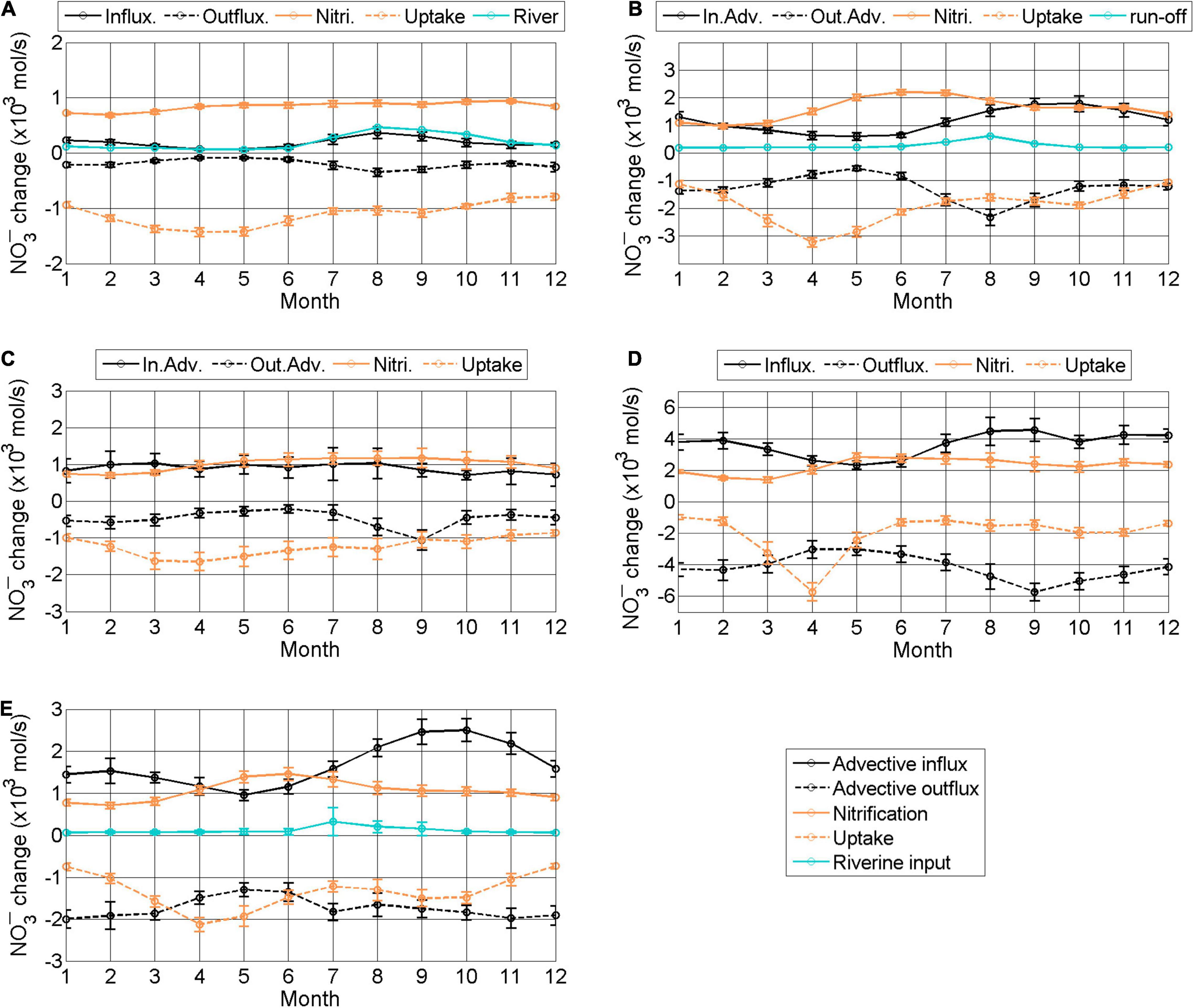
Figure 13. Monthly mean change in NO₃^– (kmols⁻¹) by advection and biological processes in different subregions averaged for the period 2006–2019. (A–E) represent subregions BS, nYS, swYS, scYS, and seYS, respectively (see Figure 11A). Black solid and dashed lines indicate total inward and outward NO₃^– fluxes via currents, respectively. Orange solid and dashed lines denote nitrification and uptake by phytoplankton, respectively. The cyan line denotes NO₃^– flux via riverine input. BS, Bohai Sea; nYS, northern Yellow Sea; swYS, southwestern Yellow Sea; scYS, southcentral Yellow Sea; seYS, southeastern Yellow Sea.

In the nYS, advective influx of NO₃^– was comparable with the change driven by biological processes in fall and winter, but was much smaller in spring and summer when uptake by phytoplankton was high (Figure 13B). The uptake consumed NO₃^– during the spring and fall blooms and nitrification supplied NO₃^– in summer because of stratification of the water column and active remineralization after the spring bloom. Total advective influx of NO₃^– was 14.0 × 10³mols⁻¹ and the outflux

was 15.2 × 10³mols⁻¹. The supply by nitrification and uptake was 19.3 × 10³ and 22.8 × 10³mols⁻¹, respectively. NO₃^– flux from the Yalu River was 3.2 × 10³mols⁻¹.

In the swYS, advective influx of NO₃^– was nearly comparable to the supply by nitrification year round (Figure 13C). The

advective outflux was lower than the uptake. The supply and consumption of NO₃^– by biological processes in the swYS were similar to those in the BS. Total advective influx and outflux were 10.8×10³ and 5.7×10³mols⁻¹, respectively, and supply by nitrification and uptake were 12.0×10³ and 14.8×10³mols⁻¹, respectively.

In the scYS, advective influx of NO₃^– was two times higher than the supply by nitrification except from April to June (Figure 13D). The advective outflux was larger than biological consumption all year except in April. Total advective influx and outflux were 44.5×10³ and 50.4×10³mols⁻¹, respectively, and the changes from nitrification and uptake yield were 27.7×10³ and 24.3×10³mols⁻¹, respectively.

NO${}_3^{-}$ in the seYS was also primarily supplied by advection, which was especially strong in fall (Figure 13E). The seasonal variation in nitrification and uptake in the seYS had a similar pattern as those in subregions nYS and scYS. Total advective influx and outflux were 20.0 × 10³ and 20.9 × 10³mols⁻¹, respectively, and the changes from nitrification and uptake yield were 12.7 × 10³ and 16.2 × 10³mols⁻¹, respectively. NO₃^– flux from rivers along the Korean coast was 1.4 × 10³mols⁻¹.

The model results clearly demonstrated that advection played a major role in the total NO₃^– budget in the central and eastern regions of the YS and that biological processes were a major factor regulating the budget in the western and northern regions of the YS and the BS. However, the relative importance of these processes varied between seasons. Notably, changes in NO₃^– driven both by currents and biological processes were essential for understanding the NO₃^– budgets and ultimately, the ecosystem in the YS and BS.

Seasonal and Spatial Variations in Nitrate Budgets

The schematic diagrams for net NO₃^– fluxes by physical and biological processes indicate the dominant factors controlling seasonal NO₃^– fluxes in each subregion (Figure 14). Net advective NO₃^– flux was anticyclonic in spring and winter but cyclonic in summer and fall following the dominant seasonal circulation patterns.

FIGURE 14

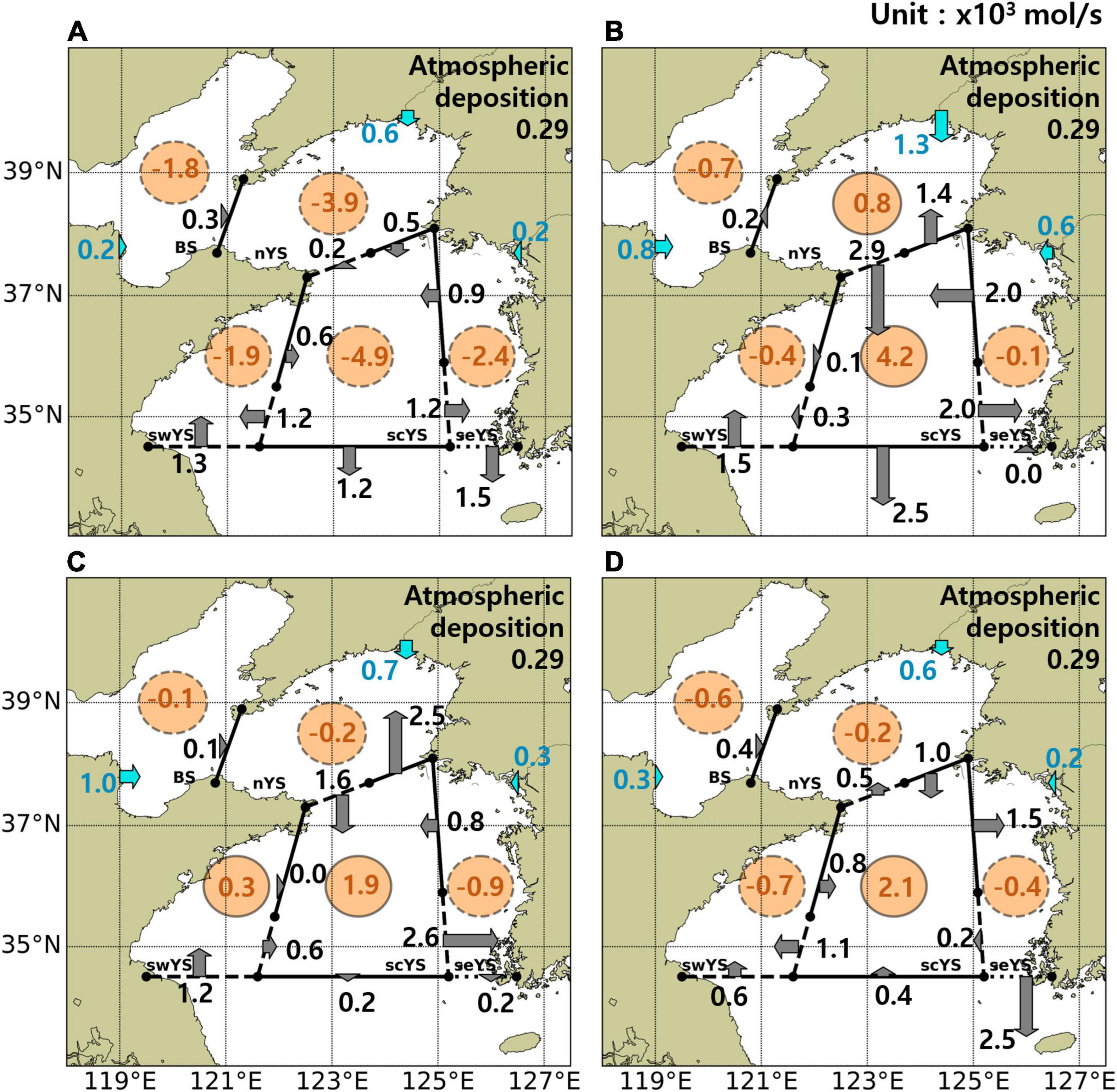
Figure 14. NO₃^– (kmols⁻¹) budgets in subregions of the YS in spring (A), summer (B), fall (C), and winter (D) averaged for the period 2006–2019. Gray arrows indicate the net advective fluxes between subregions. Cyan arrows denote the net fluxes from rivers. Orange circles denote supply (solid circle) or consumption (dashed circle) by biological processes. YS, Yellow Sea.

Net advective influx from the ECS occurred via the SCC along the Chinese coast in the swYS year round. Previous studies suggested that 0.6×10³ to 6.1×10³mols⁻¹ of DIN is transported into the swYS from the Changjiang River (Li et al., 2014, 2015), corresponding to 1.2×10³mols⁻¹ of NO₃^– from the model results. Additionally, the model results indicate that influx from the scYS into the swYS during winter and spring is also a substantial source (Figure 14). The influx of NO₃^– via the YSWC in the lower layer across the southern boundary of the scYS in winter was considerable but net flux across the boundary was very low because this flux was almost offset by the southward current-driven flux at the surface (Figure 14D). Although previous studies proposed that the YSWC could supply high NO₃^– water to the YS, the horizontal distributions from observed data (Figures 4–6) showed that a warm and saline water mass intrusion with poor NO₃^– (Jin et al., 2013; Zhou et al., 2013; Liu et al., 2015a). Moreover, the net advective influx into the scYS during winter, when the YSWC is the strongest, was insignificant. This indicates that nitrification is a more crucial source of NO₃^– in the scYS. Net advective outfluxes from the scYS occurred via the southward movement of the YSBCW in summer (Figure 14B) and from the seYS via the KCC in winter (Figure 14D). Although the advective outflux to the ECS is approximately one order of magnitude lower than other fluxes to the ECS, such as the Taiwan Warm Current, Changjiang River, and Kuroshio Current (Kim S. K. et al., 2013), it is likely to affect the southern coast of Korea because the KCC and YSBCW can flow into the southern coastal sea of Korea (Cho and Kim, 1994; Cho et al., 1995; Bae et al., 2014; Um et al., 2018). Thus, understanding the assessment of and variability in the advective outflux from the YS would be important to investigate the ecosystem over the Korean coast. Influxes of NO₃^– from the Yalu, Han, and Geum Rivers, and the atmospheric deposition were smaller than the fluxes via currents in the subregions; however, influx from the Yellow River was comparable to the advective flux in the BS where biological processes dominated the NO₃^– budget.

The consumption by phytoplankton was greater than the supply by nitrification in all subregions during spring (Figure 14A). Net consumption by biological processes continued in summer in shallow coastal regions, such as the seYS, swYS, and BS (Figure 14B), where active tidal mixing provides favorable conditions for phytoplankton by supplying nitrate to the euphotic layer (Sun and Cho, 2010). Biological uptake was lower than nitrification in offshore regions (i.e., scYS and nYS) with strong stratification in summer, which inhibited the supply of NO₃^– from the lower layer to the surface and, instead, provided a suitable environment for nitrification in the lower layer. Moreover, the advection in summer even exports NO₃^– to the ECS so that nitrification mainly results in an increase in DIN in the bottom layer of the YS, as indicated by our model results and previous observations (Supplementary Figure 1; Chen, 2009; Jin et al., 2013; Wei et al., 2016). The net supply by biological processes was the highest in the scYS during summer due to active organic matter decomposition and nitrification in the YSBCW, and the supply continued until winter. Wu et al. (2019) proposed that remineralization and nitrification are key processes to supply NO₃^– in the YSBCW. The model results also show the importance of nitrification as the source of NO₃^– and its seasonal contribution to the budgets.

Limitations of the Model

Seasonal contributions of NO₃^– budgets to biological and physical fluxes in the YS were estimated using a physical–biogeochemical numerical model. However, deficiencies in observation data and some parameterization should be improved to provide more precise assessments. In this study, organic matter was remineralized as soon as it reached the bottom layer but it is gradually decomposed depending on complicated physical and biogeochemical conditions, such as oxygen content, temperature, bacterial activity, and turbulence, in the real ocean (Glud, 2008). These conditions can vary tempo-spatially with external factors; thus, periodic and wide-ranging investigations are needed to estimate precise NO₃^– budgets.

Seasonal NO₃^– budgets from the numerical model indicated that the atmospheric flux was much lower than other sources although the flux did not consider tempo-spatial variation. However, recent studies revealed that the contribution of atmospheric deposition to NO₃^– budgets in the YS continues to increase due to anthropogenic activity (Zhang et al., 2007; Luo et al., 2018; Wang et al., 2020). Thus, the impact of a recent increase in the atmospheric deposition on budgets in the YS will be investigated through regular observation and an atmospheric-ocean coupled model.

Previous studies indicated a positive trend of NO₃^– in the southwestern YS from 2005 to 2012 but a negative trend in the southeastern YS from 2000 to 2014 (NFRDI, 2014; Li et al., 2015). Although our model results presented the same trend direction in each region, because most of the boundary conditions did not consider the inter-annual and long-term variability in our model, values of the trends from the model were different from observed data and it was difficult to determine the real causes of increased or decreased budgets. To reveal the causes of the long-term variability in nutrients due to climate change, cooperation with countries near the YS and regular investigations of the nutrient concentrations of rivers and the open ocean for the lateral boundary conditions are essential.

Summary and Conclusion

A physical-biogeochemical coupled model experiment was performed to assess the seasonal and spatial variations in NO₃^– budgets in the YS. By comparison with observation data, the model demonstrated reasonable simulation of the seasonal variations in temperature, salinity, chlorophyll-a, and NO₃^–. The model enabled us to quantitatively address the relative contribution of advective transport and biological processes in NO₃^– budgets in each subregion of the YS. Advective NO₃^– flux via currents was dominant in the central and eastern regions of the YS whereas biological flux was dominant in the western and northern regions of the YS. NO₃^– was transported cyclonically in summer and fall and anticyclonically in spring and winter following the dominant current patterns. Riverine input of NO₃^– was minor compared to the contributions of advective fluxes and biological consumption/production. The model results suggested that the SCC along the Chinese coast was a major source of NO₃^– from the ECS year round. Influx via the YSWC was offset by outflux via a southward surface current driven by the northerly wind in winter. The southward movement of the YSBCW in summer and the KCC in winter mainly drove NO₃^– export to the ECS. The influence of biological processes on NO₃^– budgets was negative in spring due to algal blooms and positive in summer due to active decomposition of organic matter and consequent nitrification. Nitrification was the largest net supplier of NO₃^– in the scYS, where the YSBCW was present.

Overall, our analyses provide initial quantitative assessment of each process including advective transport by currents, biological processes, and riverine inputs in NO₃^– budgets in the YS. Temporal and spatial variations in atmospheric deposition, sediments, and groundwater may also be important in the seasonal variation in NO₃^–; incorporation of these additional factors in future studies will further refine the model. Our study demonstrates the usefulness of the coupled model in assessing budgets of biogeochemically important parameters. This type of modeling can be adopted to address carbon transport off the shelf, for example, out of the YS in the future. In addition, causes of the annual and decadal variability in the biogeochemical processes in the YS should be investigated using the coupled model through more sophisticated model configurations.

Data Availability Statement

The original contributions presented in the study are included in the article/Supplementary Material, further inquiries can be directed to the corresponding author/s.

Author Contributions

Y-JT and Y-KC: conceptualization. Y-JT and Y-YK: methodology. Y-JT: writing draft and visualization. Y-KC and JH: review and editing. Y-KC: supervision. All authors contributed to the article and approved the submitted version.

Funding

This study was supported by the project “Deep Water Circulation and Material Cycling in the East Sea (20160400)” funded by the Ministry of Oceans and Fisheries (MOF), Republic of Korea.

Conflict of Interest

The authors declare that the research was conducted in the absence of any commercial or financial relationships that could be construed as a potential conflict of interest.

Publisher’s Note

All claims expressed in this article are solely those of the authors and do not necessarily represent those of their affiliated organizations, or those of the publisher, the editors and the reviewers. Any product that may be evaluated in this article, or claim that may be made by its manufacturer, is not guaranteed or endorsed by the publisher.

Supplementary Material

The Supplementary Material for this article can be found online at: https://www.frontiersin.org/articles/10.3389/fmars.2021.785377/full#supplementary-material

References

Bach, L. T., Riebesell, U., Sett, S., Febiri, S., Rzepka, P., and Schulz, K. G. (2012). An approach for particle sinking velocity measurements in the 3–400 μm size range and considerations on the effect of temperature on sinking rates. Mar. Biol. 159, 1853–1864. doi: 10.1007/s00227-012-1945-2

PubMed Abstract | CrossRef Full Text | Google Scholar

Bae, S. H., Kim, D. C., Lee, G. S., Kim, G. Y., Kim, S. P., Seo, Y. K., et al. (2014). Physical and acoustic properties of inner shelf sediments in the South Sea, Korea. Quat. Int. 344, 125–142. doi: 10.1016/j.quaint.2014.03.058

CrossRef Full Text | Google Scholar

Bashkin, V. N., Park, S. U., Choi, M. S., and Lee, C. B. (2002). “Nitrogen budgets for the Republic of Korea and the Yellow Sea region,” in The Nitrogen Cycle at Regional to Global Scales, eds E. W. Boyer and R. W. Howarth (Dordrecht: Springer), 387–403. doi: 10.1007/978-94-017-3405-9_12

CrossRef Full Text | Google Scholar

Beardsley, R. C., Limeburner, R., Kim, K., and Candela, J. (1992). Lagrangian flow observations in the East China, Yellow and Japan seas. La Mer 30, 297–314.

Google Scholar

Castillo-Ramírez, A., Santamaría-del-Ángel, E., González-Silvera, A., Frouin, R., Sebastiá-Frasquet, M.-T., Tan, J., et al. (2020). A new algorithm to estimate diffuse attenuation coefficient from Secchi disk depth. J. Mar. Sci. Eng. 8:558. doi: 10.3390/jmse8080558

CrossRef Full Text | Google Scholar

Chen, C. T. A. (2009). Chemical and physical fronts in the Bohai, Yellow and East China seas. J. Mar. Syst. 78, 394–410. doi: 10.1016/j.jmarsys.2008.11.016

CrossRef Full Text | Google Scholar

Chengkui, Z. (1984). Phycological research in the development of the Chinese seaweed industry. Hydrobiologia 116, 7–18. doi: 10.1007/BF00027633

CrossRef Full Text | Google Scholar

Cho, Y.-K., and Kim, K. (1994). Characteristics and origin of the cold water in the South Sea of Korea in summer. J. Korean Soc. Oceanogr. 29, 414–421.

Google Scholar

Cho, Y.-K., Kim, K., and Rho, H.-K. (1995). Salinity decrease and the transport in the South Sea of Korea in summer. J. Ocean Eng. Technol. 7, 126–134.

Google Scholar

Copernicus Climate Change Service (2017). Data from: ERA5: Fifth Generation of ECMWF Atmospheric Reanalyses of the Global Climate. European Union (EU). Available online at: https://cds.climate.copernicus.eu/cdsapp#!/home (accessed April 1, 2021).

Google Scholar

Dai, Z., Du, J., Zhang, X., Su, N., and Li, J. (2011). Variation of riverine material loads and environmental consequences on the Changjiang (Yangtze) Estuary in recent decades (1955–2008). Environ. Sci. Technol. 45, 223–227. doi: 10.1021/es103026a

PubMed Abstract | CrossRef Full Text | Google Scholar

Egbert, G. D., and Erofeeva, S. Y. (2002). Efficient inverse modeling of barotropic ocean tides. J. Atmos. Oceanic Technol. 19, 183–204.

Google Scholar

Fairall, C. W., Bradley, E. F., Rogers, D. P., Edson, J. B., and Young, G. S. (1996). Bulk parameterization of air-sea fluxes for tropical ocean-global atmosphere coupled-ocean atmosphere response experiment. J. Geophys. Res. Ocean. 101, 3747–3764. doi: 10.1029/95JC03205

CrossRef Full Text | Google Scholar

Fasham, M. J. R., Ducklow, H. W., and McKelvie, S. M. (1990). A nitrogen-based model of plankton dynamics in the oceanic mixed layer. J. Mar. Res. 48, 591–639. doi: 10.1357/002224090784984678

CrossRef Full Text | Google Scholar

Fennel, K., Wilkin, J., Levin, J., Moisan, J., O’Reilly, J., and Haidvogel, D. (2006). Nitrogen cycling in the middle Atlantic bight: results from a three-dimensional model and implications for the North Atlantic nitrogen budget. Glob. Biogeochem. Cycles 20:GB3007. doi: 10.1029/2005GB002456

CrossRef Full Text | Google Scholar

Fu, M., Sun, P., Wang, Z., Wei, Q., Qu, P., Zhang, X., et al. (2018). Structure, characteristics and possible formation mechanisms of the subsurface chlorophyll maximum in the Yellow Sea Cold Water Mass. Cont. Shelf Res. 165, 93–105. doi: 10.1016/j.csr.2018.07.007

CrossRef Full Text | Google Scholar

Fu, M., Wang, Z., Li, Y., Li, R., Sun, P., Wei, X., et al. (2009). Phytoplankton biomass size structure and its regulation in the Southern Yellow Sea (China): seasonal variability. Cont. Shelf Res. 29, 2178–2194. doi: 10.1016/j.csr.2009.08.010

CrossRef Full Text | Google Scholar

Gan, J., Lu, Z., Cheung, A., Dai, M., Liang, L., Harrison, P. J., et al. (2014). Assessing ecosystem response to phosphorus and nitrogen limitation in the Pearl River plume using the regional ocean modeling system (ROMS). J. Geophys. Res. Oceans 119, 8858–8877. doi: 10.1002/2014JC009951

CrossRef Full Text | Google Scholar

Garcia, H. E., Locarnini, R. A., Boyer, T. P., Antonov, J. I., Baranova, O. K., Zweng, M. M., et al. (2013). Data from: World Ocean Atlas 2013. Volume 4, Dissolved Inorganic Nutrients (Phosphate, Nitrate, Silicate). NOAA Atlas NESDIS 76. Silver Spring, MD: National Oceanographic Data Center, 25. doi: 10.7289/V5J67DWD

CrossRef Full Text | Google Scholar

Glud, R. N. (2008). Oxygen dynamics of marine sediments. Mar. Biol. Res. 4, 243–289. doi: 10.1080/17451000801888726

CrossRef Full Text | Google Scholar

Gong, Y., Yu, Z., Yao, Q., Chen, H., Mi, T., and Tan, J. (2015). Seasonal variation and sources of dissolved nutrients in the Yellow River, China. Int. J. Environ. Res. Public Health 12, 9603–9622. doi: 10.3390/ijerph120809603

PubMed Abstract | CrossRef Full Text | Google Scholar

Gruber, N., Frenzel, H., Doney, S. C., Marchesiello, P., McWilliams, J. C., Moisan, J. R., et al. (2006). Eddy-resolving simulation of plankton ecosystem dynamics in the California current system. Deep Sea Res. Part 1 Oceanogr. Res. Pap. 53, 1483–1516. doi: 10.1016/j.dsr.2006.06.005

CrossRef Full Text | Google Scholar

Guo, C., Zhang, G., Sun, J., Leng, X., Xu, W., Wu, C., et al. (2020). Seasonal responses of nutrient to hydrology and biology in the southern Yellow Sea. Cont. Shelf Res. 206:104207. doi: 10.1016/j.csr.2020.104207

CrossRef Full Text | Google Scholar

Holmes, R. W. (1970). The Secchi disk in turbid coastal waters. Limnol. Oceanogr. 15, 688–694. doi: 10.4319/lo.1970.15.5.0688

CrossRef Full Text | Google Scholar

Howarth, R. W. (1988). Nutrient limitation of net primary production in marine ecosystems. Ann. Rev. Ecol. 19, 89–110. doi: 10.1146/annurev.es.19.110188.000513

CrossRef Full Text | Google Scholar

Hsueh, Y. (1988). Recent current observations in the eastern Yellow Sea. J. Geophys. Res. Oceans 93, 6875–6884. doi: 10.1029/JC093iC06p06875

CrossRef Full Text | Google Scholar

Hwang, J. H., Van, S. P., Choi, B.-J., Chang, Y. S., and Kim, Y. H. (2014). The physical processes in the Yellow Sea. Ocean Coast. Manag. 102, 449–457. doi: 10.1016/j.ocecoaman.2014.03.026

CrossRef Full Text | Google Scholar

Hyun, J.-H., and Kim, K.-H. (2003). Bacterial abundance and production during the unique spring phytoplankton bloom in the central Yellow Sea. Mar. Ecol. Prog. Ser. 252, 77–88. doi: 10.3354/meps252077

CrossRef Full Text | Google Scholar

Jang, P.-G., Lee, T. S., Kang, J.-H., and Shin, K. (2013). The influence of thermohaline fronts on chlorophyll a concentrations during spring and summer in the southeastern Yellow Sea. Acta Ocean. Sin. 32, 82–90. doi: 10.1007/s13131-013-0355-8

CrossRef Full Text | Google Scholar

Jin, J., Liu, S. M., Ren, J. L., Liu, C. G., Zhang, J., Zhang, G. L., et al. (2013). Nutrient dynamics and coupling with phytoplankton species composition during the spring blooms in the Yellow Sea. Deep Sea Res. Part 2 Top. Stud. Oceanogr. 97, 16–32. doi: 10.1016/j.dsr2.2013.05.002

CrossRef Full Text | Google Scholar

Kim, C.-S., Cho, Y.-K., Choi, B.-J., Jung, K. T., and You, S. H. (2013). Improving a prediction system for oil spills in the Yellow Sea: effect of tides on subtidal flow. Mar. Pollut. Bull. 68, 85–92. doi: 10.1016/j.marpolbul.2012.12.018

PubMed Abstract | CrossRef Full Text | Google Scholar

Kim, J. K., Yarish, C., Hwang, E. K., Park, M., and Kim, Y. (2017). Seaweed aquaculture: cultivation technologies, challenges and its ecosystem services. Algae 32, 1–13. doi: 10.4490/algae.2017.32.3.3

CrossRef Full Text | Google Scholar

Kim, S. K., Chang, K. I., Kim, B., and Cho, Y. K. (2013). Contribution of ocean current to the increase in N abundance in the Northwestern Pacific marginal seas. Geophys. Res. Lett. 40, 143–148. doi: 10.1029/2012GL054545

CrossRef Full Text | Google Scholar

Kim, T. W., Lee, K., Najjar, R. G., Jeong, H.-D., and Jeong, H. J. (2011). Increasing N abundance in the Northwestern Pacific Ocean due to atmospheric nitrogen deposition. Science 334, 505–509. doi: 10.1126/science.1206583

PubMed Abstract | CrossRef Full Text | Google Scholar

Kiyomoto, Y., Iseki, K., and Okamura, K. (2001). Ocean color satellite imagery and shipboard measurements of chlorophyll a and suspended particulate matter distribution in the East China Sea. J. Oceanogr. 57, 37–44. doi: 10.1023/A:1011170619482

CrossRef Full Text | Google Scholar

Large, W. G., McWilliams, J. C., and Doney, S. C. (1994). Oceanic vertical mixing: a review and a model with a nonlocal boundary layer parameterization. Rev. Geophys. 32, 363–403. doi: 10.1029/94RG01872

CrossRef Full Text | Google Scholar

Li, H.-M., Tang, H.-J., Shi, X.-Y., Zhang, C.-S., and Wang, X.-L. (2014). Increased nutrient loads from the Changjiang (Yangtze) river have led to increased harmful algal blooms. Harmful Algae 39, 92–101. doi: 10.1016/j.hal.2014.07.002

CrossRef Full Text | Google Scholar

Li, H.-M., Zhang, C.-S., Han, X.-R., and Shi, X.-Y. (2015). Changes in concentrations of oxygen, dissolved nitrogen, phosphate, and silicate in the southern Yellow Sea, 1980–2012: sources and seaward gradients. Estuar. Coast. Shelf Sci. 163, 44–55. doi: 10.1016/j.ecss.2014.12.013

CrossRef Full Text | Google Scholar

Lie, H.-J., Cho, C.-H., Lee, J.-H., Lee, S., Tang, Y., and Zou, E. (2001). Does the Yellow Sea warm current really exist as a persistent mean flow? J. Geophys. Res. Ocean. 106, 22199–22210. doi: 10.1029/2000JC000629

CrossRef Full Text | Google Scholar

Lim, D.-I., Kang, M.-R., Jang, P.-G., Kim, S.-Y., Jung, H.-S., Kang, Y.-S., et al. (2008). Water quality characteristics along midwestern coastal area of Korea (in Korean). Ocean Polar Res. 30, 379–399. doi: 10.4217/OPR.2008.30.4.379

CrossRef Full Text | Google Scholar

Lin, X., and Yang, J. (2011). An asymmetric upwind flow, Yellow Sea Warm Current: 2. Arrested topographic waves in response to the northwesterly wind. J. Geophys. Res. Oceans 116:C04027. doi: 10.1029/2010JC006514

CrossRef Full Text | Google Scholar

Lin, X., Yang, J., Guo, J., Zhang, Z., Yin, Y., Song, X., et al. (2011). An asymmetric upwind flow, Yellow Sea Warm Current: 1. New observations in the western Yellow Sea. J. Geophys. Res. Oceans 116:C04026. doi: 10.1029/2010JC006513

CrossRef Full Text | Google Scholar

Liu, D., Keesing, J. K., He, P. M., Wang, Z. L., Shi, Y. J., and Wang, Y. J. (2013). The world’s largest macroalgal bloom in the Yellow Sea, China: formation and implications. Estuar. Coast. Shelf Sci. 129, 2–10. doi: 10.1016/j.ecss.2013.05.021

CrossRef Full Text | Google Scholar

Liu, S., and Zhang, J. (2004). Nutrient dynamics in the macro-tidal Yalujiang Estuary. J. Coast. Res. 43, 147–161.

Google Scholar

Liu, S. M., Altabet, M. A., Zhao, L., Larkum, J., Song, G. D., Zhang, G. L., et al. (2017). Tracing nitrogen biogeochemistry during the beginning of a spring phytoplankton bloom in the yellow sea using coupled nitrate nitrogen and oxygen isotope ratios. J. Geophys. Res. Biogeosci. 122, 2490–2508. doi: 10.1002/2016JG003752

CrossRef Full Text | Google Scholar

Liu, S. M., Zhang, J., Chen, S. Z., Chen, H. T., Hong, G. H., Wei, H., et al. (2003). Inventory of nutrient compounds in the Yellow Sea. Cont. Shelf Res. 23, 1161–1174. doi: 10.1016/S0278-4343(03)00089-X

CrossRef Full Text | Google Scholar

Liu, X., Chiang, K.-P., Liu, S.-M., Wei, H., Zhao, Y., and Huang, B.-Q. (2015a). Influence of the Yellow Sea warm current on phytoplankton community in the central Yellow Sea. Deep Sea Res. Part 1 Oceanogr. Res. Pap. 106, 17–29. doi: 10.1016/j.dsr.2015.09.008

CrossRef Full Text | Google Scholar

Liu, X., Huang, B., Huang, Q., Wang, L., Ni, X., Tang, Q., et al. (2015b). Seasonal phytoplankton response to physical processes in the southern Yellow Sea. J. Sea Res. 95, 45–55. doi: 10.1016/j.seares.2014.10.017

CrossRef Full Text | Google Scholar

Locarnini, R. A., Mishonov, A. V., Antonov, J. I, Boyer, T. P., Garcia, H. E., Baranova, O. K., et al. (2013). Data from: World Ocean Atlas 2013. Volume 1, Temperature. NOAA Atlas NESDIS 73. Silver Spring, MD: National Oceanographic Data Center, 40. doi: 10.7289/V55X26VD

CrossRef Full Text | Google Scholar

Luo, L., Kao, S.-J., Bao, H., Xiao, H., Xiao, H., Yao, X., et al. (2018). Sources of reactive nitrogen in marine aerosol over the Northwest Pacific Ocean in spring. Atmos. Chem. Phys. 18, 6207–6222. doi: 10.5194/acp-18-6207-2018

CrossRef Full Text | Google Scholar

Menten, L., and Michaelis, M. I. (1913). Die kinetik der invertinwirkung. Biochem. Z. 49, 333–369.

Google Scholar

Morel, A., and Berthon, J. F. (1989). Surface pigments, algal biomass profiles, and potential production of the euphotic layer: relationships reinvestigated in view of remote-sensing applications. Limnol. Oceanogr. 34, 1545–1562. doi: 10.4319/lo.1989.34.8.1545

CrossRef Full Text | Google Scholar

Moskilde, E. (1996). Topics in Non-Linear Dynamics: Application to Physics, Biology and Economic Systems. Hackensack, NJ: World Scientific.

Google Scholar

NFRDI (2014). Study on the Chlorosis Phenomena in Cultivated Phyropia. Annual Report of National Fisheries Research and Development Institute. Quezon City: National Fisheries Research and Development Institute.

Google Scholar

Park, M., Shin, S. K., Do, Y. H., Yarish, C., and Kim, J. K. (2018). Application of open water integrated multi-trophic aquaculture to intensive monoculture: a review of the current status and challenges in Korea. Aquaculture 497, 174–183. doi: 10.1016/j.aquaculture.2018.07.051

CrossRef Full Text | Google Scholar

Ryther, J. H., and Dunstan, W. M. (1971). Nitrogen, phosphorous, and eutrophication in the coastal marine environment. Science 171, 1008–1013. doi: 10.1126/science.171.3975.1008

PubMed Abstract | CrossRef Full Text | Google Scholar

Seo, G.-H., Cho, Y.-K., Choi, B.-J., Kim, K.-Y., Kim, B., and Tak, Y.-J. (2014). Climate change projection in the Northwest Pacific marginal seas through dynamic downscaling. J. Geophys. Res. Oceans 119, 3497–3516. doi: 10.1002/2013JC009646

CrossRef Full Text | Google Scholar

Shchepetkin, A. F., and McWilliams, J. C. (2005). The regional oceanic modeling system (ROMS): a split-explicit, free-surface, topography-following-coordinate oceanic model. Ocean Model. 9, 347–404. doi: 10.1016/j.ocemod.2004.08.002

CrossRef Full Text | Google Scholar

Shi, J., Liu, Y., Mao, X., Guo, X., Wei, H., and Gao, H. (2017). Interannual variation of spring phytoplankton bloom and response to turbulent energy generated by atmospheric forcing in the central Southern Yellow Sea of China: satellite observations and numerical model study. Cont. Shelf Res. 143, 257–270. doi: 10.1016/j.csr.2016.06.008

CrossRef Full Text | Google Scholar

Shi, W., and Wang, M. (2012). Satellite views of the Bohai Sea, Yellow Sea, and East China Sea. Prog. Oceanogr. 104, 30–45. doi: 10.1016/j.pocean.2012.05.001

CrossRef Full Text | Google Scholar

Shim, J. H., Hwang, J. R., Lee, S. Y., and Kwon, J. (2014). Variations in nutrients & CO₂ uptake rates of porphyra yezoensis ueda and a simple evaluation of in situ N & C demand rates at aquaculture farms in South Korea (in Korean). Korean J. Environ. Biol. 32, 297–305. doi: 10.11626/KJEB.2014.32.4.297

CrossRef Full Text | Google Scholar

Siswanto, E., Tang, J., Yamaguchi, H., Ahn, Y.-H., Ishizaka, J., Yoo, S., et al. (2011). Empirical ocean-color algorithms to retrieve chlorophyll-a, total suspended matter, and colored dissolved organic matter absorption coefficient in the Yellow and East China Seas. J. Oceanogr. 67, 627–650. doi: 10.1007/s10872-011-0062-z

CrossRef Full Text | Google Scholar

Smayda, T. J. (1969). Some measurements of the sinking rate of fecal pellets. Limnol. Oceanogr. 14, 621–625. doi: 10.4319/lo.1969.14.4.0621

CrossRef Full Text | Google Scholar

Song, G., Liu, S., Zhu, Z., Zhai, W., Zhu, C., and Zhang, J. (2016). Sediment oxygen consumption and benthic organic carbon mineralization on the continental shelves of the East China Sea and the Yellow Sea. Deep Sea Res. Part 2 Top. Stud. Oceanogr. 124, 53–63. doi: 10.1016/j.dsr2.2015.04.012

CrossRef Full Text | Google Scholar

Sun, Y.-J., and Cho, Y.-K. (2010). Tidal front and its relation to the biological process in coastal water. Ocean Sci. J. 45, 243–251. doi: 10.1007/s12601-010-0022-3

CrossRef Full Text | Google Scholar

Tan, S.-C., and Shi, G.-Y. (2012). The relationship between satellite-derived primary production and vertical mixing and atmospheric inputs in the Yellow Sea cold water mass. Cont. Shelf Res. 48, 138–145. doi: 10.1016/j.csr.2012.07.015

CrossRef Full Text | Google Scholar

Tak, Y.-J., Cho, Y.-K., and Nam, S. (2020). Numerical investigation of the generation of continental shelf waves and their role in the westward shift of the Yellow Sea Warm Current. Prog. Oceanogr. 187:102404. doi: 10.1016/j.pocean.2020.102404

CrossRef Full Text | Google Scholar

Tak, Y.-J., Cho, Y.-K., Seo, G.-H., and Choi, B.-J. (2016). Evolution of wind-driven flows in the Yellow Sea during winter. J. Geophys. Res. Oceans 121, 1970–1983. doi: 10.1002/2016JC011622

CrossRef Full Text | Google Scholar

Teague, W. J., and Jacobs, G. A. (2000). Current observations on the development of the Yellow Sea Warm Current. J. Geophys. Res. Oceans 105, 3401–3411. doi: 10.1029/1999JC900301

CrossRef Full Text | Google Scholar

Uda, M. (1934). Hydrographical research on the normal monthly conditions in the Japan Sea, the Yellow Sea, and the Okhotsk Sea. J. Imp. Fish. Exp. Sta. 5, 191–236.

Google Scholar

Uitz, J., Claustre, H., Morel, A., and Hooker, S. B. (2006). Vertical distribution of phytoplankton communities in open ocean: an assessment based on surface chlorophyll. J. Geophys. Res. Oceans 111:C08005. doi: 10.1029/2005JC003207

CrossRef Full Text | Google Scholar

Um, I. K., Choi, M. S., Bae, S. H., Song, Y., and Kong, G. S. (2018). Provenance of fine-grained sediments in the inner shelf of the Korea Strait (South Sea), Korea. Ocean Sci. J. 53, 31–42. doi: 10.1007/s12601-017-0062-z

CrossRef Full Text | Google Scholar

Vörösmarty, C. J., Fekete, B., and Tucker, B. A. (1996). Data from: River Discharge Database, Version 1.0 (RivDIS v1. 0), Volumes 0 through 6. A contribution to IHP-V Theme: 1. Technical Documents in Hydrology Series. Paris: UNESCO.

Google Scholar

Wang, B., Wang, X., and Zhan, R. (2003). Nutrient conditions in the Yellow Sea and the East China Sea. Estuar. Coast. Shelf Sci. 58, 127–136. doi: 10.1016/S0272-7714(03)00067-2

CrossRef Full Text | Google Scholar

Wang, J., Beusen, A. H. W., Liu, X., Van Dingenen, R., Dentener, F., Yao, Q., et al. (2020). Spatially explicit inventory of sources of nitrogen inputs to the Yellow Sea, East China Sea, and South China Sea for the period 1970–2010. Earths Future 8:e2020EF001516. doi: 10.1029/2020EF001516

CrossRef Full Text | Google Scholar

Wang, K., Chen, J. F., Jin, H. Y., Chen, F. J., Li, H. L., Gao, S. Q., et al. (2011). The four seasons nutrients distribution in Changjiang River Estuary and its adjacent East China Sea. J. Mar. Sci. 29, 18–35.

Google Scholar

Wang, Q., Guo, X., and Takeoka, H. (2008). Seasonal variations of the Yellow River plume in the Bohai Sea: a model study. J. Geophys. Res. Oceans 113:C08046. doi: 10.1029/2007JC004555

CrossRef Full Text | Google Scholar

Wei, Q.-S., Yu, Z.-G., Wang, B.-D., Fu, M.-Z., Xia, C.-S., Liu, L., et al. (2016). Coupling of the spatial–temporal distributions of nutrients and physical conditions in the southern Yellow Sea. J. Mar. Syst. 156, 30–45. doi: 10.1016/j.jmarsys.2015.12.001

CrossRef Full Text | Google Scholar

Wu, H., Gu, J., and Zhu, P. (2018). Winter counter-wint transport in the inner southwestern Yellow Sea. J. Geophys. Res. Oceans 123, 411–436. doi: 10.1002/2017JC013403

CrossRef Full Text | Google Scholar

Wu, Z., Yu, Z., Song, X., Wang, W., Zhou, P., Cao, X., et al. (2019). Key nitrogen biogeochemical processes in the South Yellow Sea revealed by dual stable isotopes of nitrate. Estuar. Coast. Shelf Sci. 225:106222. doi: 10.1016/j.ecss.2019.05.004

CrossRef Full Text | Google Scholar

Xing, Q., Yu, H., Yu, H., Sun, P., Liu, Y., Ye, Z., et al. (2020). A comprehensive model-based index for identification of larval retention areas: a case study for Japanese anchovy Engraulis japonicus in the Yellow Sea. Ecol. Indic. 116:106479. doi: 10.1016/j.ecolind.2020.106479

CrossRef Full Text | Google Scholar

Xuan, J.-L., Zhou, F., Huang, D.-J., Wei, H., Liu, C.-G., and Xing, C.-X. (2011). Physical processes and their role on the spatial and temporal variability of the spring phytoplankton bloom in the central Yellow Sea. Acta Ecol. Sin. 31, 61–70. doi: 10.1016/j.chnaes.2010.11.011

CrossRef Full Text | Google Scholar

Yamaguchi, H., Kim, H.-C., Son, Y. B., Kim, S. W., Okamura, K., Kiyomoto, Y., et al. (2012). Seasonal and summer interannual variations of SeaWiFS chlorophyll a in the Yellow Sea and East China Sea. Prog. Oceanogr. 105, 22–29. doi: 10.1016/j.pocean.2012.04.004

CrossRef Full Text | Google Scholar

Yanagi, T., and Takahashi, S. (1993). Seasonal variation of circulations in the East China Sea and the Yellow Sea. J. Oceanogr. 49, 503–520. doi: 10.1007/BF02237458

CrossRef Full Text | Google Scholar

Yang, H.-W., Cho, Y.-K., Seo, G.-H., You, S. H., and Seo, J.-W. (2014). Interannual variation of the southern limit in the Yellow Sea bottom cold water and its causes. J. Mar. Syst. 139, 119–127. doi: 10.1016/j.jmarsys.2014.05.007

CrossRef Full Text | Google Scholar

Yuan, D., Li, Y., Wang, B., He, L., and Hirose, N. (2017). Coastal circulation in the southwestern Yellow Sea in the summers of 2008 and 2009. Cont. Shelf Res. 143, 101–117. doi: 10.1016/j.csr.2017.01.022

CrossRef Full Text | Google Scholar

Zhang, J. (1994). Atmospheric wet deposition of nutrient elements: correlation with harmful biological blooms in Northwest Pacific coastal zones. Ambio 23, 464–468.

Google Scholar

Zhang, G., Zhang, J., and Liu, S. (2007). Characterization of nutrients in the atmospheric wet and dry deposition observed at the two monitoring sites over Yellow Sea and East China Sea. J. Atmos. Chem. 57, 41–57. doi: 10.1007/s10874-007-9060-3

CrossRef Full Text | Google Scholar

Zhao, B., Yao, P., Bianchi, T. S., Arellano, A. R., Wang, X., Yang, J., et al. (2018). The remineralization of sedimentary organic carbon in different sedimentary regimes of the Yellow and East China Seas. Chem. Geol. 495, 104–117. doi: 10.1016/j.chemgeo.2018.08.012

CrossRef Full Text | Google Scholar

Zhou, F., Chai, F., Huang, D., Xue, H., Chen, J., Xiu, P., et al. (2017). Investigation of hypoxia off the Changjiang Estuary using a coupled model of ROMS-CoSiNE. Prog. Oceanogr. 159, 237–254. doi: 10.1016/j.pocean.2017.10.008

CrossRef Full Text | Google Scholar

Zhou, F., Xuan, J., Huang, D., Liu, C., and Sun, J. (2013). The timing and the magnitude of spring phytoplankton blooms and their relationship with physical forcing in the central Yellow Sea in 2009. Deep Sea Res. Part 2 Top. Stud. Oceanogr. 97, 4–15. doi: 10.1016/j.dsr2.2013.05.001

CrossRef Full Text | Google Scholar

Zweng, M. M., Reagan, J. R., Antonov, J. I., Locarnini, R. A., Mishonov, A. V., Boyer, T. P., et al. (2013). Data From: World Ocean Atlas 2013. Volume 2, Salinity. NOAA Atlas NESDIS 74. Silver Spring, MD: National Oceanographic Data Center, 39. doi: 10.7289/V5251G4D

CrossRef Full Text | Google Scholar