 Siim Pärt
 Harri Kankaanpää
 Jan-Victor Björkqvist
 Rivo Uiboupin
- 1Department of Marine Systems, Tallinn University of Technology, Tallinn, Estonia
- 2Marine Research Centre, Finnish Environment Institute, Helsinki, Finland
- 3Norwegian Meteorological Institute, Bergen, Norway
- 4Finnish Meteorological Institute, Helsinki, Finland
A large part of oil spills happen near busy marine fairways. Presently, oil spill detection and monitoring are mostly done with satellite remote sensing algorithms, or with remote sensors or visual surveillance from aerial vehicles or ships. These techniques have their drawbacks and limitations. We evaluated the feasibility of using fluorometric sensors in flow-through systems for real-time detection of oil spills. The sensors were capable of detecting diesel oil for at least 20 days in laboratory conditions, but the presence of CDOM, turbidity and algae-derived substances substantially affected the detection capabilities. Algae extract was observed to have the strongest effect on the fluorescence signal, enhancing the signal in all combinations of sensors and solutions. The sensors were then integrated to a FerryBox system and a moored SmartBuoy. The field tests support the results of the laboratory experiments, namely that the primary source of the measured variation was the presence of interference compounds. The 2 month experiments data did not reveal peaks indicative of oil spills. Both autonomous systems worked well, providing real-time data. The main uncertainty is how the sensors' calibration and specificity to oil, and the measurement depth, affects oil detection. We recommend exploring mathematical approaches and more advanced sensors to correct for natural interferences.
1. Introduction
Oil spills are a major threat to the marine ecosystems, local communities and economy (Samiullah, 1985; Farrington, 2014; Jørgensen et al., 2019; Câmara et al., 2021; Sandifer et al., 2021). The research into the consequences of oil pollution has been long and extensive. The effects to wildlife are broad, ranging from exposure of birds (Jenssen, 1994; Stephenson, 1997; Fox et al., 2016) and mammals (Engelhardt, 1987; Bodkin et al., 2002; Ridoux et al., 2004) to oil to toxic, mutagenic and/or carcinogenic effects of polycyclic aromatic hydrocarbons (PAHs) present in crude oil and products based on fossil oil (Hylland, 2006; Abdel-Shafy and Mansour, 2016; Hayakawa, 2018; Honda and Suzuki, 2020). Besides harming the natural environment, oil spills can impair the economy in the affected region (Cohen, 1993; Taleghani and Tyagi, 2017; Ribeiro et al., 2021) and have adverse effects on human health and psychology (D'Andrea and Reddy, 2014; Shultz et al., 2015; Sandifer et al., 2021).
The Baltic Sea has always been an important route for maritime trade and transport, accounting for up to 15% of the world's maritime traffic (HELCOM, 2003; WWF, 2010). Oil shipments in the Baltic Sea are projected to grow by 64% by 2030, from about 180 million tons to nearly 300 million tons (HELCOM, 2018a) and the overall volume of ship traffic has been estimated to double during the period 2010–2030 (Rytkönen et al., 2002). The immense volume of shipping in the Baltic Sea is accompanied by a high risk of accidents. According to the Helsinki Commission (HELCOM), 1,520 maritime accidents have occurred in the Baltic Sea area during the period 2011–2015, with a fairly stable rate of 300 accidents per year; 4% of these accidents led to loss of life, serious injuries or environmental damages (HELCOM, 2018a).
A considerable contributor to marine oil pollution is oil pollution by ships, which are concentrated to main shipping lanes and other areas of high maritime activity (Serra-Sogas et al., 2008; Ferraro et al., 2009; Liubartseva et al., 2015; Sankaran, 2019; Polinov et al., 2021). It is estimated that in the Baltic Sea 10% of the total amount of oil hydrocarbons comes from illegal discharges by vessels (HELCOM, 2003). These various smaller spills, referred to as operational oil spills, are not the result of ship accidents, but instead result from discharges of small amounts of oil, or more usually unfiltered oily water. Most of this pollution risk is concentrated along major ship routes (HELCOM, 2013). The number and size of these spills has been decreasing (HELCOM, 2018c). For example, in 2015 the number of observed spills was 80 and the total estimated annual volume of oil spills observed in 2009–2015 was in the order of 20 m3 (HELCOM, 2018a). However, even small amounts of oil can have a negative impact on the marine environment (Brussaard et al., 2016).
Current oil spill remote sensing methods have become more reliable but they still have many drawbacks and limitations (Fingas and Brown, 2018). Nowadays the most dominant and cost-effective means for remote spill detection is the combination of satellite-based synthetic aperture radar (SAR) images and aircraft surveillance flights for verification (Gade et al., 2000; Uiboupin et al., 2008; Solberg, 2012; Fingas and Brown, 2018). SAR sensors give a good coverage and are not limited by cloud cover or weather conditions. Furthermore, there are many studies on algorithms meant for identification of oil spills from SAR data (Marghany, 2016; Krestenitis et al., 2019; Al-Ruzouq et al., 2020; Zeng and Wang, 2020). Besides SAR, optical remote sensing techniques gathering information in different spectral range (ultraviolet, visible, and near-infrared) and can give useful information about oil pollution (Solberg, 2012; Fingas and Brown, 2018; Al-Ruzouq et al., 2020). Ships and aircraft equipped with radar or optical sensor are also widely used for detection and monitoring of oil pollution (Jensen et al., 2008; Xu et al., 2020). Also, sensors like microwave radiometers and laser fluorometers mounted on aircraft can provide additional information about the oil type and amount (Jha et al., 2008; Solberg, 2012).
Oil spills can be difficult to detect even with modern aerial surveillance equipment for numerous reasons. They can be small, and in rough sea the oil is mixed well below the surface, while a visible slick might also disappear because of evaporation. Optical methods of satellite sensing are also limited by resolution, cloud cover and the sea state (Brekke and Solberg, 2005; Jha et al., 2008; Fingas and Brown, 2018). Even the most studied and used remote sensing method of detecting oil from SAR images has problems, such as lookalikes—radar signatures similar to oil pollution but which can actually be for example floating algae, ship wakes, cold upwelling water or natural surface films produced by plankton or fish (Sipelgas and Uiboupin, 2007; Alpers et al., 2017; Al-Ruzouq et al., 2020). Even a comprehensive satellite coverage might therefore not be able to detect all oil spills. Nonetheless, PAHs will remain in the water after the spill is no longer visible on the surface but are still detectable by in-water fluorometers. Thus, the real-time detection of these spills would benefit from additional detection systems. In addition, in-situ sensors can be used for validation for remote sensing techniques and vice versa. One possible in-situ solution is to use fluorometric sensors installed on a suitable platform.
Ships of Opportunity (SOOPs) fitted with oceanographic instrumentation and automated water sampling systems, so-called FerryBoxes, are commonly used for studies of near surface waters (Petersen et al., 2003, 2011; Hydes et al., 2010; Petersen, 2014). Also, the Baltic Sea is well covered with FerryBox lines (Petersen, 2014; Schneider et al., 2014; Karlson et al., 2016; Kikas and Lips, 2016). FerryBoxes have a great potential for gathering scientific data, especially when installed on ferries and cargo ships cruising the same route on a regular basis. While SOOPs give a good spatial coverage, monitoring buoys give an excellent temporal coverage. Such autonomous monitoring buoy systems are being developed and operated worldwide to measure the physical and biogeochemical properties of coastal surface waters (Mills et al., 2003; Nam et al., 2005). The technological progress has resulted in SmartBuoys with a stable power supply, two-way communication and real-time data acquisition for effective environmental monitoring (Chavez et al., 1997; Mills et al., 2003; Nam et al., 2005; Benson et al., 2008; Papoutsa et al., 2012). Moroni et al. (2016) have developed a sensorized buoy for detecting oil spills from the air-side. Fluorescence-based in-situ sensors and systems have been globally used for real-time monitoring of oil spills and determining the levels of the contamination (Lambert et al., 2001, 2003; He et al., 2003; Kim et al., 2010; Malkov and Sievert, 2010; Tedetti et al., 2010). Combining FerryBoxes and SmartBuoys with portable fluorometric sensors could provide an additional method for early notification of oil spills in the sea. Nonetheless, to our knowledge, such an approach has not previously been adopted.
Fluorometric detection (FLD) is essentially about measuring fluorescence at predetermined wavelengths, meaning that FLD can't resolve between different sources of hydrocarbons and fluorescent compounds – for example oil and oil refined products, combustion processes (e.g., power plants, maritime and land-based traffic, forest fires). Compound-specific laboratory methods such as gas chromatography–mass spectrometry can make such distinctions, but field-usability (data continuity), speed and low running costs still make FLD-based field protocols appealing alternatives compared to laboratory-based techniques.
For purposes of the operational detection of oil spills, the accuracy of the sensor is a crucial, but not the sole part. We split up the operational chain of oil-detection with fluorometers to five steps: 1) the sensors need to accurately and selectively detect oil, 2) the system where the sensors are operating need to function at least semi-autonomously, 3) the system needs to reliably transmit real time data, 4) an automated algorithm detects anomalic events and 5) the data is available to the user in a reliable interface on a short notice. In this study we focus on steps 1–3 and 5. We first present laboratory tests of sensors and then evaluate the real-time oil detection capability of two autonomous in-situ remote sensing platforms that are equipped with fluorometers. The two platforms, a FerryBox and a SmartBuoy, covered high-risk areas in the Baltic Sea.
2. Materials and Methods
2.1. UviLux, EnviroFlu-HC 500 and Turner Design C3 Fluorometers
Three commercially available fluorometric instruments, designed for in-situ and real-time quantification of oil or oil compounds, were chosen for the experiments: UviLux and EnviroFlu-HC 500 for the FerryBox system, and C3 Submersible Fluorometer for the SmartBuoy. All three sensors were also tested in laboratory conditions.
The UviLux UV-fluorometer (Chelsea Technologies Ltd, UK) is an in-situ UV fluorometer. Oil detection is based on the measurement of PAH concentrations. The sensitivity of the sensor is 0.005 μg carbazole per liter, the calibrated range is 0.005–2,000 μg carbazole per liter, the excitation wavelength is 255 nm, and the emission wavelength is 360 nm.
The EnviroFlu-HC 500 submersible UV fluorometer (TriOS Optical Sensors, Germany) is an instrument designed for the measurement of PAHs in water. The fluorometer has a minimum detection limit of 0.3 μg phenantrene per liter, a calibrated range of 0–500 μg phenantrene per liter, an excitation wavelength 254 nm, and an emission wavelength of 360 nm.
The Turner Design C3 submersible fluorometer (Turner Design, USA) is manufactured according to users' requirements. C3 fluorometers come with a factory-installed temperature probe and can be configured with up to three optical sensors. Each optical sensor is designed with fixed excitation and emission filters. For the SmartBuoy experiment the C3 fluorometer was equipped with three sensors: a hydrocarbon sensor for crude oil with sensitivity of 0.2 μg pyrenetetrasulfonic acid (PTSA) per liter and linear range 0–1500 μg PTSA per liter, excitation light 325/120 nm and emission light 410–600 nm; a sensor for colored dissolved organic matter (CDOM) with minimum detection limit (MDL) 0.1 μg quinine sulfate per liter, linear range 0–1.5 μg quinine sulfate per liter, excitation wavelength 325–120 nm and emission wavelength 470–60 nm; a turbidity sensor with MDL 0.05 Nephelometric Turbidity Units (NTU) and range 0–1,500 NTU, excitation wavelength 850 nm, and emission wavelength 850 nm.
2.2. Laboratory Tests
In order to examine selectivity and sensitivity of fluorometric sensors to oil, two separate laboratory experiments were performed in 2017. All experiments were performed in a dark climatic room set to a temperature of 16°C.
The first experiment examined the selectivity of the sensors, i.e., interferences to oil detection caused by interfering substances. Baltic Sea water (S; salinity 6.2 PSU) was used as a blank and as a solution for extraction of humic substances (H), cyanobacterial algae (A) and production of clay suspension (C).
Stock solutions (one of each) of clay suspension (from Baltic Sea's clayey sediment), seawater extract of humic substances (originating from decayed plant material) and a seawater extract of cyanobacterial algae (from dried Baltic Sea surface phytoplankton) were produced. Also, two batches of water accommodated fraction (WAF; W) of diesel oil were produced. Each extract was made by combining 100 ml of commercial winter-quality diesel oil with 1,000 ml of seawater under gentle stirring overnight. All solutions were prepared 1 week prior to measurements in the aquarium. Concentrations of PAHs were quantified using gas chromatography—mass spectrometry and aliphatic hydrocarbons (decane-tetracontane) using gas chromatography—flame ionization detection at SYKE laboratory center. No attempt was made to determine chemical composition of each interference solution in detail, instead the solutions mimicked natural constituents in Baltic Sea water.
Altogether six glass beakers (each 2,000 ml) were wrapped with black plastic except for the top section and filled with 1,200 ml of seawater. Aliquots of the clay suspension (50.0 ml), humic extract (50.0 ml), cyanobacteria algae extract (10.0 ml) and diesel WAF (50 ml) were sequentially added so that all combinations of the aforementioned solutions in seawater were achieved. The solutions were kept in slow stirring motion using a magnetic stirrer. In first three sets of measurements no WAF was added. WAF was applied in three last measurement sets. After addition of each solution the responses were measured using one sensor at a time at exactly 50 mm below the upper level of the beakers. The top part of the beakers and the sensor housing were wrapped with black plastic. Fluorescence responses were collected for 3–5 min with each sensor and the average and standard deviation of fluorescence for each period of data collection were calculated.
The logging rates used with fluorometer sensors during the experiment were 1 min (average of values collected at 0.5 Hz), 30 and 1 s for the UviLux, EnviroFlu-HC and Turner C3 sensors, respectively. Data from EnviroFlu-HC were logged into a laptop PC using the TriOS MSDA_XE software and the data from Turner C3 into a PC using Turner C-soft software. Data from UviLux were logged into a portable logger connected to automatic GSM network-based modem and sent via GSM network to Tallinn University of Technology once a minute. Altogether 1.32 million, 79,000 and 30,000 time points of data from Turner C3, Enviroflu-HC and UviLux were generated, respectively. The small dilution effect in WAF solutions, caused by the volume increase by the added interference solutions, was compensated by a corresponding multiplier factor in final calculations thus yielding oil-related fluorescence (ORF) presented. Normalized responses from each fluorometer were calculated by dividing observed responses from different solutions with responses obtained from seawater. No compensation was calculated for CDOM or turbidity values.
The second experiment for diesel WAF persistence and for method comparison lasted for 3 weeks. A 25-liter glass aquarium was used and placed over a black plastic sheet in a steel tank and filled with 21.8 liters of filtered seawater (salinity 6.2 PSU). Thermostatted (11°C) tap water was circulated in the exterior tank. The FLD sensors were fixed into laboratory stands so that the optical window of each sensor was at 10 cm below the surface of liquid (Figure 1). Gentle mixing was applied using an electricity-powered laboratory stirrer. The aquarium was covered by a black plastic wrapping except during water sampling and maintenance. The UviLux sensor needed to be moved further away from the two other sensors due to interference that was unfortunately not noticed before 7 days into the experiment. The data transmission, storage and sensors' acquisition rates were as described for the first experiment.
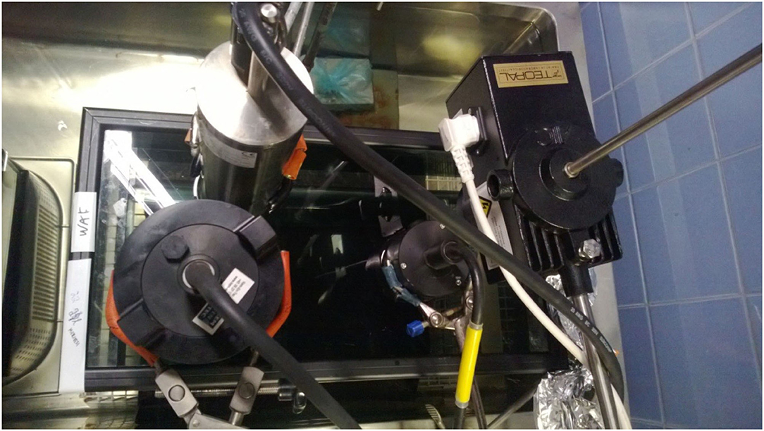
Figure 1. Above view of the experimental set up. Instruments: TriOS EnviroFlu-HC (with metallic cover, upper part), Turner C3 (with black cover, left) and UviLux (black cover, right). The electric motor of the stirrer is at far right. Photograph: Harri Kankaanpää.
The persistence of diesel oil fractions in seawater and comparability between oil detection methods were measured in the second test. The methods were: the three fluorometric sensors, total oil monitoring method used by Finland, gas chromatography flame ionization detection (GC–FID; for aliphatic hydrocarbons) and gas chromatography—mass spectrometry (GC–MS; for PAHs including 1– and 2–methylnapthtalene). At S1–S9, water samples of 100 ml were collected for total oil HELCOM protocol and another 100 ml for the GC–MS and GC–FID analyses.
The Finnish HELCOM monitoring method for total oil analysis can be described briefly as follows: seawater is extracted with 10 ml of n–hexane under stirring. Fluorescence is measured using 310 and 360 nm excitation and emission wavelengths, respectively. Calibration is performed using solutions of Norwegian crude oil (Ekofisk) dissolved in n–hexane. Limit of quantification is 0.05 μg oil/l and analytical error is ±15%.
Aliphatic hydrocarbons (decane-tetracontane) were extracted using n-hexane, cleaned up using adsorbent, concentrated, separated using gas chromatography and quantified by flame ionization detection. The method has a limit of quantification of 100 μg total aliphatics/l and analytical error of 30 %. PAHs were extracted using n-hexane under stirring or solid phase extraction. The n-hexane solution was then concentrated and analyzed using GC–MS. The quantification limits of the method were between 0.005 and 0.01 μg/l, while the analytical errors varied between 20 and 40% depending on compound.
Normalized responses for each detection method were calculated by dividing observed responses with period S1 responses at given water sampling time points (S1–S9).
2.3. FerryBox Operation and Oil Detection Capability
A FerryBox system developed by Marine Systems Institute at Tallinn University of Technology is used on board of the M/S Baltic Queen (Tallink Group, Estonia) (Figure 2), which commutes between Tallinn (Estonia), Mariehamn (Åland) and Stockholm (Sweden) (Figure 3). The ship route covers the western Gulf of Finland, Northern Baltic Proper, Southern Archipelago Sea, and Southern Åland Sea (Figure 3). One crossing, including a stop in Mariehamn harbor, is about 425 km long and takes approximately 17 h. The ship then returns after a 7 h stay in the destination harbor.
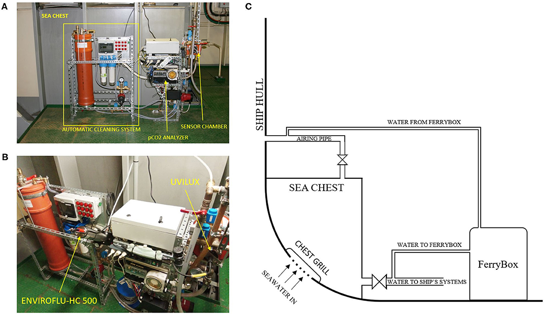
Figure 2. FerryBox system on board M/S Baltic Queen (A) and the same system with UviLux and EnviroFlu-HC fluorometers during the experiment (B). General scheme of the FerryBox's placement and water flow on M/S Baltic Queen is shown on figure (C). Photographs: Kaimo Vahter.
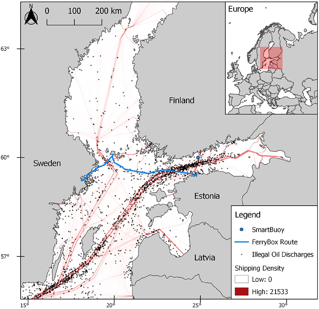
Figure 3. FerryBox line and SmartBuoy mooring location in the Baltic Sea. Points of information describing the location and size of illegal oil discharges observed during aerial surveillance flights by HELCOM Contracting Parties during 1998–2017 (HELCOM, 2018b). Shipping density (defined as the number of ships crossing a 1 × 1 km grid cell) of all IMO (International Maritime Organization) registered ships operating in the Baltic Sea in 2016 (HELCOM, 2017).
All FerryBoxes are flow-through systems where the water is taken in from an inlet in a vessel hull and then pumped into a measuring circuit containing sensors (Petersen, 2014). On M/S Baltic Queen the water was taken from the ship's sea chest and pumped continuously through the FerryBox system at a rate of 9 l/min. The opening of the chest is situated about 4 m below the waterline. Parameters were measured with 1-min intervals, giving an approximately 0.5 km spatial resolution along the fairway, depending on the ship's speed. A typical transect contained roughly 1,000 records for each variable.
The UviLux and EnviroFlu-HC fluorometers, were installed in parallel to the FerryBox system (Figure 2B), which recorded additional real-time seawater properties. Conductivity (salinity) and temperature was measured with a High-Precision Pressure Level Transmitter Series 36XiW (KELLER AG, Switzerland), turbidity was measured with a Seapoint Turbidity Meter (Seapoint Sensors Inc., USA) and pCO2 was measured with an OceanPackTM pCO2 analyzer (SubCtech, Germany).
We made four maintenance visits to M/S Baltic Queen in order to clean the FerryBox system and the sensors. These visits were made roughly every 2 weeks (March 3, March 20, April 3, April 15) during our 2-month experiment (February 21 to April 21, 2018). The maintenance consisted of washing the system with a solution of oxalic acid and a manual cleaning of the optical sensors. The FerryBox also has a automatic cleaning system, which was not functional during the experiment. Similar automatic acid-washing cleaning method is applied to prevent biofouling on a FerryBox traveling between Tallinn and Helsinki (Lips et al., 2016).
Measurements from the sensors in the FerryBox were collected by a datalogger (RTCU-MX2i pro by Logic IO) on board M/S Baltic Queen. The datalogger includes a modem and a GPS, and adds the position and a time stamp to the measurement before sending the data to an on-shore FTP server of the Marine Systems Institute using the GSM/GPRS protocol. The data were sent in real-time (every minute).
A publicly available, web-based, user interface was built to visualize the data online, where the ship's track, real-time position and gathered FerryBox data was available in real-time (Figure 4) (TalTech, 2017). The web-based user interface is also equipped with different options to view historical data: the user can select parameters or time periods, and construct a map view and 2D graphs of multiple parameters. Data are also available in a tabulated form and parameters can be viewed in color-coded view along the ship's track. The data that were provided in real-time during the experiment is still available on the web-page.
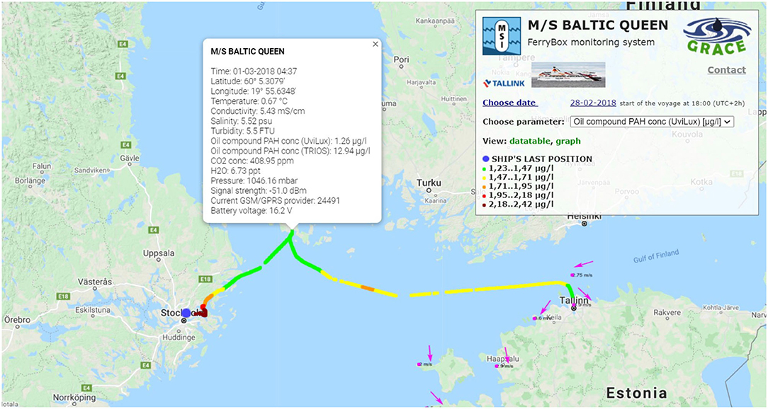
Figure 4. Web-based user interface for viewing the real-time data from the FerryBox system (TalTech, 2017). The gaps in the data were caused by loss of the GSM-network.
2.4. SmartBuoy Setup and Experiment for Oil Spill Detection
The SmartBuoy, developed by Meritaito Ltd (Finland), is a combination of a polyethylene spar buoy with mobile and/or satellite communication technology and a versatile selection of monitoring sensors (Figure 5). The Turner Design C3 fluorometer was installed inside of the buoy in a vertical monitoring well with an open flow through a pipe, enabling continuous sea water exchange. The monitoring depth was 2–3 m depending on the sea level. Concentration of CDOM and turbidity values were measured simultaneously with the hydrocarbon measurements. To ensure high data quality, the C3 sensor was equipped with a mechanical wiper cleaning all three optical lenses before taking the measurements. In addition to the water quality monitoring, the SmartBuoy also collected data about current speed and direction at the depth of 7 m to identify spreading direction of potential oil spills. Furthermore, the significant wave height was calculated from roughly 8.5-min time series, measured by a pressure sensor (Aanderaa Wave and Tide Sensor 5218).
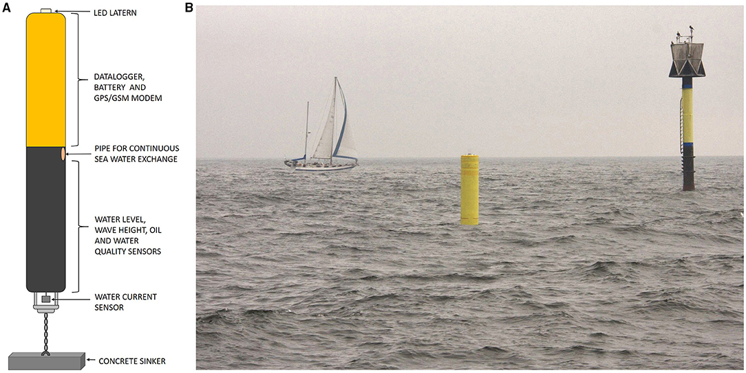
Figure 5. Schematic figure of the SmartBuoy system (A) and the SmartBuoy deployed to the off-shore area in the Gulf of Finland for oil spill detection (B). Photograph: Joose Mykkänen.
Water quality and sea state sensors were connected to a datalogger (Aanderaa SmartGuard 5300) that was programmed to operate the sensors with an 1-h measurement and data transmission interval. Real-time data from the SmartBuoy were transmitted over satellite modem to a server, where it were subjected to an automatic data quality control before being visualized online.
The SmartBuoy buoy was moored on a junction of the main merchant shipping lanes in the Gulf of Finland (Figure 3) for a 2-month measurement period (October 25 to December 24, 2018). Vessels navigating on the north–south direction shipping lane between Helsinki and Tallinn were passing close to the buoy, and vessels on the east–west direction shipping lane passed the buoy further south. The SmartBuoy was visited once during the monitoring period for datalogger reprogramming and manual maintenance of the sensors.
3. Results of the Laboratory Experiments
The produced WAF contained the following main PAH constituents (all μg/l): naphthalene (65), 1-methylnapthtalene (89), 2-methylnapthtalene (31), anthracene (1.6), acenaphthene (2.7), acenaphthylene (1.2), phenanthrene (1.2), fluoranthene (0.20), fluorene (4.4) and pyrene (0.2). Other PAHs fell below the 0.005 μg/l limit of quantification. The concentration of aliphatic compounds was 1,200 μg/l.
3.1. Effect of Interference Solutions
In the first laboratory experiment we investigated how the sensors reacted to the addition of interference solutions. In the absence of interference solutions, Turner C3 showed the largest absolute fluorescence values (primary data), followed by Enviroflu-HC and Uvilux. The data from Turner C3's PAH and CDOM channels had occasional spikes, but overall the data stability from each channel of the detectors were good. When WAF was added to the seawater, the relative change in signal strength (normalized response) was largest for UviLux (4.48-fold), followed by EnviroFlu-HC (2.62-fold) and Turner C3 (1.1-fold) (Table 1).
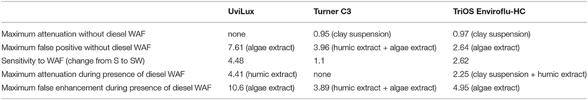
Table 1. Relative responses (fold compared to average fluorescence in seawater) of sensors to interference solutions, sensitivity to water accommodated fraction (WAF) of diesel oil.
All sensors reacted when interference solutions were added to seawater. The addition of suspended clay to seawater slightly attenuated the PAH channel's fluorescence signal in Turner C3 and Enviroflu-HC, while slightly enhancing it in UviLux (Figure 6, left half, S vs. SC). When suspended clay was added to the seawater-WAF solution, the signal was slightly attenuated in Enviroflu-HC and UviLux, and slightly enhanced in Turner C3 (Figure 6, right half, SW vs. SWC). In all combinations, the changes were at most 12% (0.88–1.04).
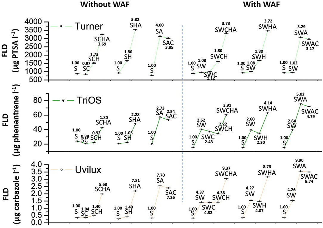
Figure 6. Fluorescence responses from EnviroFlu-HC (TriOS), Turner C3 (Turner) and UviLux sensors in seawater, seawater containing interferences of clay, humic substances, algae substances, and seawater containing diesel WAF with and without the interferences. S = seawater, C = clay suspension, H = humic substance extract, A = cyanobacterial algae extract, and W = water accommodated fraction (diesel fuel extracted in seawater). PTSA = 1,3,6,8-pyrenetetrasulphonic acid tetrasodium salt. The change in FLD response respective to the baseline (S) value in each series (e.g., S–SC–SCH–SCHA) is indicated on top of each treatment.
The sensors were more sensitive to the presence of humic substance extracts, with the PAH-signals increasing between 1.05- and 1.8-fold in all sensors (compared to seawater). The enhancement was strongest in Turner C3 and weakest in EnviroFlu-HC (Figure 6, left half, S vs. SH). In the seawater-WAF solution the added humic extracts enhanced the PAH signal in Turner C3 (1.67-fold), while slightly attenuating the signal in the other sensors (Figure 6, right half, SW vs. SWH).
Clearly the largest effect on the PAH fluorescence signal was observed after adding algae extract. The signal was enhanced in all combinations of sensors and solutions. Importantly, the enhancement caused by the algae extract was stronger than the PAH signal of the WAF-solution without any interference solutions, which means that the presence of algae can interfere strongly with the sensors ability to detect oil compounds in the water. The enhancements when adding the algae extract to the seawater were roughly between 3- and 8-fold, with UviLux showing the largest change and EnviroFlu-HC showing the smallest change (Figure 6, right half, SW vs. SWA). When the algae extract was added to the seawater-WAF solution, the PAH signal was enhanced roughly 2- to 3-fold in all sensors, with Turner C3 showing the strongest change in signal strength (Figure 6, right half, SW vs. SWA).
3.2. Diesel WAF Persistence and Method Comparison
In the second laboratory experiment we studied how long the sensors can detect oil compounds in seawater, while also comparing detection methods. Lagging software caused several gaps in the Turner C3 data and one gap in the EnviroFlu-HC data. UviLux was relocated after 165 h when we noted that it did not react clearly to the third addition of WAF (WAF3; Figure 7), having large subsequent oscillations in the signal. This behavior was caused by optical interference by the two other sensors. Despite that there was substantial suppression in UviLux responses during the suppressed period, the sensor overall did show slight responses even during this period. These small responses occurred simultaneously when adding WAF 1 and WAF 3 (but not when adding WAF 2), and were also simultaneous with HELCOM and Enviroflu-HC responses (Figure 7). After UviLux was relocated, it provided data with a considerably higher response and less noise. For response calculations we therefore only used the UviLux data gathered after the relocation.
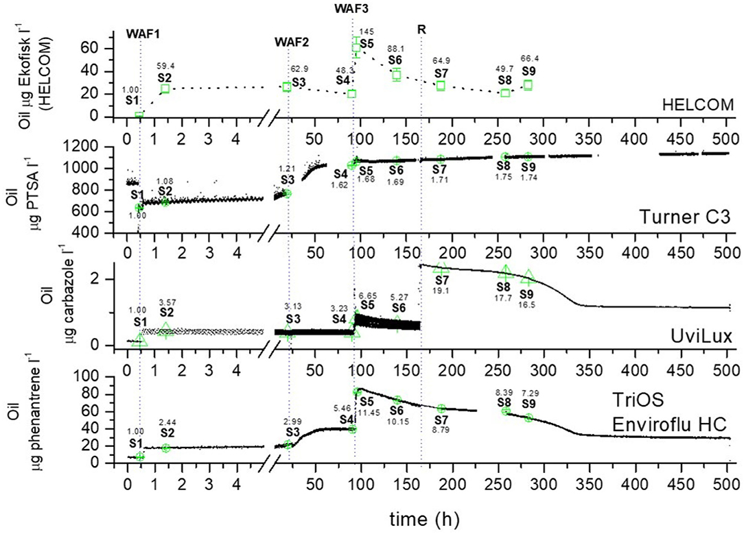
Figure 7. Evolution of responses of fluorescence signals obtained in experiment two over 503.2 h originating from HELCOM reference method (top), Turner C3, UviLux and EnviroFlu-HC (bottom). S1–S9: water sampling events; WAF1–WAF3: events of WAF addition; R: relocation of the sensors. Normalized response values relative to the initial background level (at S1) measured before just before S events are indicated above each S event.
The responses from all sensors and the standard HELCOM oil monitoring method indicated that fluorescent compounds originating from diesel oil were detectable for at least 20 days since the start of the experiment (Figure 7). The temporal evolution in PAH-related responses measured by the EnviroFlu-HC and UviLux sensors were in line with the HELCOM method, especially after the readjustment of the sensors. In contrast, Turner C3 showed slightly increasing fluorescence between 100 and 505 h while the signal from the other two sensors decayed and leveled off.
Table 2 summarizes the responses obtained from sensor-based fluorescence right before water samples (GC methods) were collected at events S5 and S7. Event before sample S7 should serve as the primary point for response comparison since it was taken after the readjustment of sensor locations (R). The relative responses compared to initial state S1 of the fluorescence-based methods, during 165–505 h were (from strongest to weakest): HELCOM, UviLux, EnviroFlu-HC and Turner C3 (Figure 7 including responses at each S event).
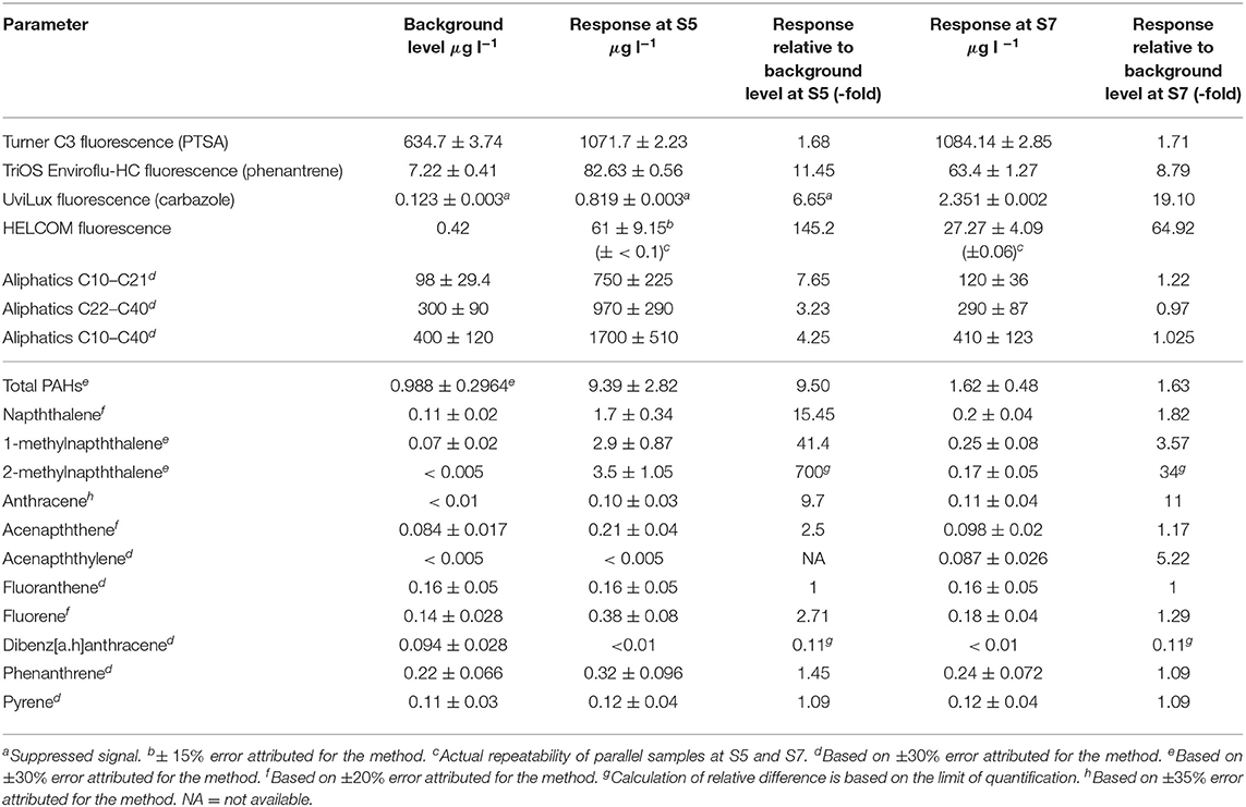
Table 2. Overview on the response levels generated by the fluorescence-based methods and parameters obtained from GC–FID and GC–MS analyses.
Several PAH molecules were good indicators for diesel-originating contamination (Table 2). All napthtalenes provided pronounced responses also at S1 (strongest to weakest): 1-methylnaphtalene (1-MN), naphthalene (NAF) and 2-methylnaphtalene (2-MN) (data not shown). Also, anthracene, acenapthtene and phenantrene were sensitive and showed a similar temporal evolution as the FLD-based responses and the methylated napthtalenes (1/2-MN).
Concentration of fluoranthene did not change over the experimental period, and Dibenz[a.h]anthracene showed a declining trend compared to the initial seawater (Figure 8). These substances (in addition to acenapthtylene, fluoranthene, dibenzo[a,h]anthracene and pyrene) were poor proxies for WAF contamination in the seawater (Figure 8).
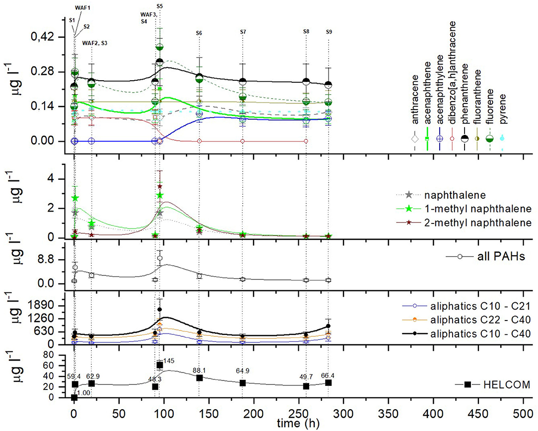
Figure 8. Concentrations of hydrocarbon compounds analyzed using GC–FID (aliphatic hydrocarbons) and GC–MS (PAHs) from samples of experiment two. The values on top of HELCOM data points denote signal relative to baseline. S1–S9 are water sampling events and WAF1–WAF3 events of WAF addition.
The concentration of aliphatic hydrocarbons followed a similar pattern as those of FLD, methylated napthtalene and the more sensitive PAHs. The PAH and aliphatic hydrocarbon concentrations also had a similar evolution pattern as the values derived using the HELCOM fluorescence method. Interestingly, the increase in aliphatic hydrocarbon concentrations between S8 and S9 showed a similar increase as the HELCOM method; this change was not visible in any other parameter (Figures 7, 8).
4. Results of the Field Experiments
4.1. FerryBox Experiment
The real-time transmission and online presentation of the FerryBox data worked well, but data gaps occurred systematically in the Baltic Proper due to loss of the GSM network. These gaps typically lasted a maximum of a few hours. An example is presented in Figure 4. The complete data was recovered from the datalogger after the fact. Altogether 58 ship voyages were analyzed. The PAH-transects were visually checked for peaks that would have indicated an oil pollution. No such anomalies were found during the 2-month measurement period the UviLux and EnviroFlu-HC fluorometers were installed to the FerryBox system.
The detected PAH values stayed between 1 and 2.6 μg carbazole/l for the UviLux and 12.4–25.5 μg phenantrene/l for the EnviroFlu-HC (Figures 9A,B). The detected hydrocarbon values were lowest in the sea areas near Åland and highest in the Stockholm archipelago, where the effect of the natural background of organic carbon from river waters is greater (Figures 9A,B). From 20.5°, longitude eastward, the PAH values were quite homogeneous. Some variation can be seen e.g., between 22°, and 23° longitude (trips 19–23), showing up more clearly in the UviLux data (Figures 9A,B). We surmise that the detected values do not reflect concentration of carbazole, phenantrene or oil in seawater. This interpretation is supported by the chemical monitoring (HELCOM/EU MSFD) and analysis of the Baltic Sea, which has found concentrations below 1 μg oil hydrocarbons/l rather constantly (Pikkarainen and Lemponen, 2005; FIMR and Olsonen, 2007). These low values are considered to be typical for seawater without significant oil pollution (Bícego et al., 1996; Zanardi et al., 1999).
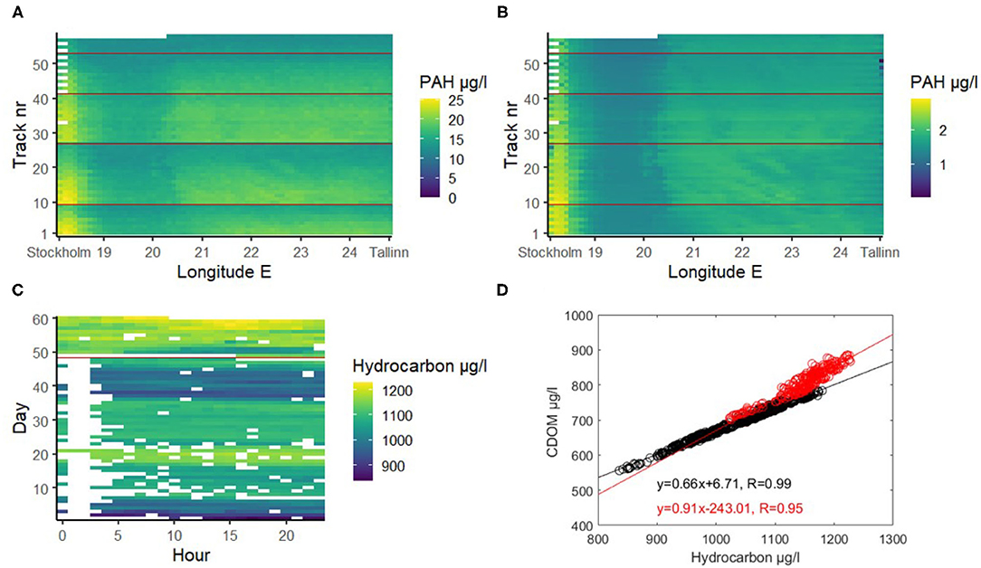
Figure 9. Heatmap plots showing spatiotemporal distributions of PAH concentrations in seawater along the ship track between Stockholm and Tallinn (February 21 to April 21, 2018) measured with the UviLux (A) and EnviroFlu-HC (B) fluorometric sensors. A temporal heatmap of the SmartBuoy data (October 25 to December 24, 2018) (C) and correlation between CDOM and hydrocarbon data before (black) and after (red) the maintenance (D). Red lines on the heatmaps indicate system maintenance visits.
The FerryBox and the accompanying sensors were maintained and cleaned frequently. Nevertheless, biofouling still impacted the quality of the measured data as can be seen from the decreasing values between the maintenance visits (Figures 9A,B). The field data suggests that EnviroFlu-HC is affected more strongly by the fouling than UviLux.
4.2. SmartBuoy Experiment
The obtained values ranged between 790 and 1,250 during the monitoring period. The variation pattern was nearly identical with the variation of collected colored organic carbon (CDOM) values, varying between 600 and 890 (Figure 9). The measured data had systematic gaps. On the 12th of December a maintenance visit to the boy was made to reprogram the datalogger and manually clean the sensors.
The correlation between the collected hydrocarbon dataset and the CDOM data set collected by the C3 sensor on SmartBuoy was very high (Figure 9D). No anomalic spikes indicative of oil-contamination were present during the test period. The C3 sensor on SmarBuoy was equipped with a mechanical wiper, which cleaned all three optical lenses prior to measuring. No significant reduction in data quality due to biofouling was detected compared to the FerryBox where the detected values gradually decreased after the cleaning (Figure 9). The linear relationship between the two variables changed after the maintenance on 12 December. This change was probably caused by the readjustment of the mechanical wipers (Joose Mykkänen, Personal communication). Nonetheless, the correlation between the variables remained high (Figure 9D).
During the experimental period, the buoy tolerated several events with significant wave heights over 2 m. The maximum significant wave height reached almost 3 m, which is estimated to be exceeded at this location roughly 1% of the times (Tuomi et al., 2011; Björkqvist et al., 2018). During the monitoring period the current speed reached 39 cm/s, with the mean value being 12 cm/s. The mean yearly current speed (for depth 0–7.5 m) in the area is expected to be under 10 cm/s (Westerlund et al., 2018).
5. Discussion
Laboratory tests showed that optical interferences strongly affected optical PAH detection. The effect of these interferences was corroborated by the strong correlation between oil-related fluorescence and CDOM fluorescence (Figure 9D). CDOM causes interference and false positives whenever it is present sufficiently and not accounted for properly. Similar results arose from the presence of cyanobacteria-derived material. The Baltic Sea contains substantial concentrations of CDOM at any time of year, most prominently close to river outlets. The quenching of oil-related fluorescence caused by clay-derived turbidity further complicates the interpretation of the signal.
Extensive spring and summer blooms of phytoplankton occur regularly in the Baltic sea (Kahru et al., 2007, 2016; Groetsch et al., 2014). We can also suspect greater interference during summer blooms of cyanobacteria and minor contribution throughout the year as there are always small quantities of chlorophylls and phycocyanin of phytoplankton origin in the surface waters. The spring bloom duration in the Baltic Sea is about one and a half months (Groetsch et al., 2016) and the peak of the bloom in 2018 coincided with the end of the FerryBox experiment (Almén and Tamelander, 2020). Nevertheless, we did not see the signal enhancing effect of the phytoplankton during the FerryBox experiment, as the PAH signals should have increased toward the end of the testing period together with the bloom intensity.
There also exist several overall issues when using fluorometers that are related to the information about the presence and relative concentration of oil compounds in water. Fluorometers are generally calibrated using a specific oil or specific compounds; thus, the relevant concentration results are relative to the specific oil or compound and the procedure used to calibrate the instrument (Lambert et al., 2003). The response of the fluorometer to oil depends significantly on the oil composition and its weathering state, complicating the quantification of oil concentration further (Henry et al., 1999). Also other studies have noted that the other fluorescent substances in seawater can significantly interfere with direct fluorescence measurements of petroleum hydrocarbons (Henry et al., 1999; Bugden et al., 2008; Tedetti et al., 2010; Cyr et al., 2019). Lastly, a reliable comparison of different sensors would also require a consensus over the units used to report FLD-based results.
Taking account of the aforementioned issues and the knowledge that most of the oil pollution in the Baltic Sea comes from small operational oil spills, and that most cases requiring criminal prosecution have involved diesel oil, the latter was selected to mimic the oil pollution in our laboratory experiments. Moreover, based on this background and the results of the laboratory tests, the field trials concentrated only on the detection of oil pollution, which should have appeared as a clear peak, deviating from the background fluorescence in the measured response patterns. The question of capabilities to detect different types of oil in the field is not only a question of the detection capabilities of the actual sensors, since also the weathering process for e.g., crude oil and diesel oil differ. In addition, the calibration of the sensors can reflect the a priori expectations of what type of oil might be encountered. It is therefore impossible to give any general recommendations on this subject, and follow-up studies are needed to test the suitability of the sensors used in this study in case they are planned to be used outside the Baltic Sea.
Due to the interfering substances it is difficult to distinguish water quality variations from the responses from oil spills. To combat that problem, suitable mathematical protocols should be explored. Some newer sensors also include built-in correction methods to discriminate oil from the natural interferences. Examples of sensors with such specification are Vlux OilPro (Chelsea Technologies Ltd), SeaOWL UV-A™ (Sea-Bird Scientific) and HM-900 (Pyxis).
Another aspect that needs careful consideration is the measurement or water intake depth of the oil detection systems. After a spill, wind, waves and currents can break the oil spill into droplets and may propel the oil deeper into the water column; this process is called natural dispersion. Dispersion is a complicated physio–chemical process affected by the characteristics of the oil spill (oil type, density, viscosity, thickness) and other seawater properties such as temperature and salinity (Xiankun et al., 1993; Papadimitrakis et al., 2011). Various other physical, chemical, and biological processes begin to alter the oil as well, altogether referred to as weathering process (Mishra and Kumar, 2015; Tarr et al., 2016).
Using sampling and further laboratory analysis the maximum detection depths of naturally dispersed oils has been between 2.5 and 15 m (Cormack and Nichols, 1977; Lichtenthaler and Daling, 1983, 1985). An experiment by Cormack and Nichols (1977), part of which was monitoring naturally dispersed Ekofisk crude oil in the water column, showed comparatively rapid decrease in oil concentration down to 5 m depth, followed by a slower decrease to background levels at 20 m. A similar experiment in Norwegian waters with 10 m3 of topped Statfjord crude oil showed that small concentrations of oil were present to at least at a depth of 3 m in the water column under the slick (Lichtenthaler and Daling, 1985). In another experiment done with 2,000 liters of Statfjord crude oil and of topped Statfjord crude oil the maximum detection depths were 2.5 m (Lichtenthaler and Daling, 1983).
At the Baffin Island Oil Spill experimental site in the Canadian Arctic, flow-through fluorometry was successfully used to monitor a subsurface release of chemically dispersed crude oil cloud over several days, providing real-time and continuous data on oil concentrations in the water column (Green et al., 1983). Nonetheless, during a surface release experiment performed in the same study, petroleum hydrocarbons from the untreated oil were not detected in the water column deeper than 1 m (Humphrey et al., 1987). In a contained oil spill experiment, part of which was 3 liters of crude oil spilled in moored 66 m3 containers in the ocean, a continuous flow-through fluorescence system was capable of detecting oil concentrations down to 8 m, over a period of 7 days (Green et al., 1982). Lunel (1995), using continuous-flow fluorometry (calibrated using discrete samples) found traces of oil down to 5 m after 20 metric ton of a mixture of medium fuel oil and gas oil (in a 50–50 ratio) were experimentally released in United Kingdom waters. Nevertheless, these experiments made in U.K., the Canadian Arctic and inside the British Colombian archipelago might not be directly transferable to the Baltic Sea because of differences in hydrography, and wind and wave conditions.
The probability of detecting oil pollution clearly depends on the weather conditions, and the size, oil type, source and weathering state of the spill. Most of the FerryBox systems are limited to a fixed depth set by the ship's design, as is the case in this study. For the FerryBox system on M/S Baltic Queen, the water is taken in at a depth of approximately 4 m and the SmartBuoy sensors situate 2–3 m below the surface, depending on the sea level. In light of the results of the aforementioned studies, these depths should be suitable for detecting anomalies in fluorescence. Also, for the FerryBox the water will also be mixed by the moving ship itself. Nonetheless, when devising such systems in the future, measurement depths as close to the surface as possible are recommended to ensure higher chance of spill detection.
Biofouling (marine growth) is likewise a major factor limiting the reliability of optical sensors in aquatic studies, especially during long term measurements. Biofouling is the net result of various physical, chemical and biological factors such as water temperature, conductivity, season, and location—to name a few (Delauney et al., 2010). Several antifoulant approaches for optical systems on autonomous platform have been suggested (Manov et al., 2004; Delauney et al., 2010). In our experiments the automatic mechanical cleaning of the sensor on the SmartBoy was satisfactory but the fouling of the FerryBox sensors after the maintenance visits is clearly there. It is not evident how much biofouling affects the oil detection capabilities of the sensors, but in our experiment is seemed to be of secondary importance compared to the presence of the other interfering substances.
6. Conclusions
Laboratory experiments indicated that the sensitivity of the sensors to diesel oil is good and they provide useful data on oil in seawater. Fluorescent compounds from the oil were detectable by the fluorometric sensors for at least 20 days. Our laboratory tests were conducted with diesel oil, Baltic Sea water, and local interfering substances and therefore may not be representative of different types of oils or marine areas. The main issue with the sensors we used was their specificity, since the presence of humic substances (CDOM), phytoplankton (phycocyanin and chlorophylls) or high turbidity (suspended/colloidal clay) can cause false positives or signal quenching when detecting oil. In our tests the impact of algal material was clearly the most significant. We suggest exploring mathematical protocols or use of more sophisticated sensors for distinguishing actual oil pollution from co-occurring optical interference.
The three tested portable fluorometers were successfully integrated to the FerryBox and SmartBuoy systems. The systems functioned semi-autonomously well during the 2-month testing periods, as did the real-time data transmissions and user interfaces/data visualization. The signal quenching effect of the biofouling could be seen on the FerryBox fluorometers, but it was a secondary problem compared to the interfering substances in the seawater. Nonetheless, automatic cleaning methods of the systems and sensors are recommended.
In this paper we did not touch upon the automatic detection of the anomalic events in the detected values that would indicate an oil spill, but this kind of an algorithm should be developed if the detection system is to be used operationally. When these systems can reliably detect oil, a comprehensive network of SmartBuoys and FerryBoxes covering the major fairways can greatly complement the aerial surveillance, ship-based and satellite monitoring that are presently used to, among other things, detect oil in seawater.
Data Availability Statement
The raw data supporting the conclusions of this article will be made available by the authors, without undue reservation. The data received from the real-time transmission of the FerryBox system can be viewed on a public web-site (TalTech, 2017).
Author Contributions
SP: investigation, validation, formal analysis, writing—original draft, and visualization. HK: methodology, investigation, formal analysis, writing—original draft, and visualization. J-VB: validation, writing—review and editing, and supervision. RU: writing—review and editing and supervision. All authors contributed to the article and approved the submitted version.
Funding
This manuscript has been produced within project GRACE, which received funding from the European Union's Horizon 2020 research and innovation programme under Grant agreement no. 679266 and supported by the Estonian Research Council (Grant no. PSG22).
Conflict of Interest
The authors declare that the research was conducted in the absence of any commercial or financial relationships that could be construed as a potential conflict of interest.
Publisher's Note
All claims expressed in this article are solely those of the authors and do not necessarily represent those of their affiliated organizations, or those of the publisher, the editors and the reviewers. Any product that may be evaluated in this article, or claim that may be made by its manufacturer, is not guaranteed or endorsed by the publisher.
Acknowledgments
We gratefully acknowledge the contributions of Tarmo Kõuts, who was the head of work package 1 (Oil spill detection, monitoring, fate and distribution) in the GRACE project and did the original conceptualization of the FerryBox experiment. We want to thank AS Tallink Grupp for allowing us to use the FerryBox installation of their vessel for the purposes of this study. Furthermore, we would like to thank Kaimo Vahter for his contribution to the installation and upkeep of the FerryBox system, and for transfer and technical advice on the UviLux. We also appreciate the work done by the employees of Arctia Meritaito Oy and Luode Consulting Oy in carrying out the SmartBuoy experiment, and thank them for providing the consequent data and for lending instrumentation (TriOS HC-500 and Turner C3), especially Joose Mykkänen from Luode Consulting is thanked for providing technical assistance during the campaign. Jari Nuutinen and Helena Kutramoinen are thanked for the GC–MS and GC–FID analyses. Furthermore, we also wish to acknowledge help by Jere Riikonen (SYKE MRC) in laboratory experiments and Kirsten Jørgensen (SYKE MRC) acting as coordinator of GRACE.
References
Abdel-Shafy, H. I., and Mansour, M. S. (2016). A review on polycyclic aromatic hydrocarbons: source, environmental impact, effect on human health and remediation. Egypt. J. Petroleum 25, 107–123. doi: 10.1016/j.ejpe.2015.03.011
Almén, A. K., and Tamelander, T. (2020). Temperature-related timing of the spring bloom and match between phytoplankton and zooplankton. Mar. Biol. Res. 16, 674–682. doi: 10.1080/17451000.2020.1846201
Alpers, W., Holt, B., and Zeng, K. (2017). Oil spill detection by imaging radars: challenges and pitfalls. Remote Sens. Environ. 201, 133–147. doi: 10.1016/j.rse.2017.09.002
Al-Ruzouq, R., Gibril, M. B. A., Shanableh, A., Kais, A., Hamed, O., Al-Mansoori, S., et al. (2020). Sensors, features, and machine learning for oil spill detection and monitoring: a review. Remote Sens. 12, 1–42. doi: 10.3390/rs12203338
Benson, B., Chang, G., Spada, F., Manov, D., and Kastner, R. (2008). “Real-time telemetry options for ocean observing systems,” in European Telemetry Conference (Munich), 5.
Bícego, M. C., Weber, R. R., and Ito, R. G. (1996). Aromatic hydrocarbons on surface waters of Admiralty Bay, King George Island, Antarctica. Mar. Pollut. Bull. 32, 549–553. doi: 10.1016/0025-326X(96)84574-7
Björkqvist, J.-V., Lukas, I., Alari, V., van Vledder, G. P., Hulst, S., Pettersson, H., et al. (2018). Comparing a 41-year model hindcast with decades of wave measurements from the Baltic Sea. Ocean Eng. 152, 57–71. doi: 10.1016/j.oceaneng.2018.01.048
Bodkin, J. L., Ballachey, B. E., Dean, T. A., Fukuyama, A. K., Jewett, S. C., McDonald, L., et al. (2002). Sea otter population status and the process of recovery from the 1989 'Exxon Valdez' oil spill. Mar. Ecol. Prog. Ser. 241, 237–253. doi: 10.3354/meps241237
Brekke, C., and Solberg, A. H. (2005). Oil spill detection by satellite remote sensing. Remote Sens. Environ. 95, 1–13. doi: 10.1016/j.rse.2004.11.015
Brussaard, C. P., Peperzak, L., Beggah, S., Wick, L. Y., Wuerz, B., Weber, J., et al. (2016). Immediate ecotoxicological effects of short-lived oil spills on marine biota. Nat. Commun. 7:11206. doi: 10.1038/ncomms11206
Bugden, J. B. C., Yeung, C. W., Kepkay, P. E., and Lee, K. (2008). Application of ultraviolet fluorometry and excitation–emission matrix spectroscopy (EEMS) to fingerprint oil and chemically dispersed oil in seawater. Mar. Pollut. Bull. 56, 677–685. doi: 10.1016/j.marpolbul.2007.12.022
Câmara, S. F., Pinto, F. R., da Silva, F. R., Soares, M. D. O., and De Paula, T. M. (2021). Socioeconomic vulnerability of communities on the Brazilian coast to the largest oil spill (2019–2020) in tropical oceans. Ocean Coastal Manag. 202:105506. doi: 10.1016/j.ocecoaman.2020.105506
Chavez, F. P., Pennington, J. T., Herlien, R., Jannasch, H., Thurmond, G., and Friederich, G. E. (1997). Moorings and drifters for real-time interdisciplinary oceanography. J. Atmos. Ocean. Technol. 14, 1199–1211. doi: 10.1175/1520-0426(1997)014andlt;1199:MADFRTandgt;2.0.CO;2
Cohen, M. J. (1993). Economic impact of an environmental accident: a time-series analysis of the exxon valdez oil spill in southcentral alaska. Sociol. Spectrum 13, 35–63. doi: 10.1080/02732173.1993.9982016
Cormack, D., and Nichols, J. A. (1977). The concentrations of oil in sea water resulting from natural and chemically induced dispersion of oil slicks. Int. Oil Spill Conf. Proc. 1977, 381–385. doi: 10.7901/2169-3358-1977-1-381
Cyr, F., Tedetti, M., Besson, F., Bhairy, N., and Goutx, M. (2019). A glider-compatible optical sensor for the detection of polycyclic aromatic hydrocarbons in the marine environment. Front. Mar. Sci. 6:110. doi: 10.3389/fmars.2019.00110
D'Andrea, M. A., and Reddy, G. K. (2014). Crude oil spill exposure and human health risks. J. Occup. Environ. Med. 56, 1029–1041. doi: 10.1097/JOM.0000000000000217
Delauney, L., Compare, C., and Lehaitre, M. (2010). Biofouling protection for marine environmental sensors. Ocean Sci. 6, 503–511. doi: 10.5194/os-6-503-2010
Engelhardt, F. (1987). “Assessment of the vulnerability of marine mammals to oil pollution,” in Fate and Effects of Oil in Marine Ecosystems, eds J. Kuiper and W. Van den Brink (Dordrecht: Martinus Nijhoff Publishers), 101–115.
Farrington, J. W. (2014). Oil pollution in the marine environment II: Fates and effects of oil spills. Environment 56, 16–31. doi: 10.1080/00139157.2014.922382
Ferraro, G., Meyer-Roux, S., Muellenhoff, O., Pavliha, M., Svetak, J., Tarchi, D., et al. (2009). Long term monitoring of oil spills in European seas. Int. J. Remote Sens. 30, 627–645. doi: 10.1080/01431160802339464
F. I. M. R, and Olsonen, R. (2007). FIMR Monitoring of the Baltic Sea Environment-Annual Report 2006. Technical Report 59, The Finnish Institute of Marine Research.
Fingas, M., and Brown, C. E. (2018). A review of oil spill remote sensing. Sensors 18, 1–18. doi: 10.1007/978-1-4939-2493-6_732-4
Fox, C. H., O'Hara, P. D., Bertazzon, S., Morgan, K., Underwood, F. E., and Paquet, P. C. (2016). A preliminary spatial assessment of risk: Marine birds and chronic oil pollution on Canada's Pacific coast. Sci. Total Environ. 573, 799–809. doi: 10.1016/j.scitotenv.2016.08.145
Gade, M., Scholz, J., and von Viebahn, C. (2000). On the detectability of marine oil pollution in European marginal waters by means of ERS SAR imagery. Int. Geosci. Remote Sens. Sympos. 6, 2510–2512. doi: 10.1109/IGARSS.2000.859623
Green, D., Humphrey, B., and Fowler, B. (1983). The use of flow-through fluorometry for tracking dispersed oil. Int. Oil Spill Conf. 1983, 473–475. doi: 10.7901/2169-3358-1983-1-473
Green, D. R., Bucley, J., and Humphrey, B. (1982). Fate of Chemically Dispersed Oil in the Sea, A Report on Two Field Experiments. Environment Protection Service Report EPS 4-EC-82-5. Environmental Impact Control Directorate, Canada.
Groetsch, P. M. M., Simis, S. G. H., Eleveld, M. A., and Peters, S. W. M. (2014). Cyanobacterial bloom detection based on coherence between ferrybox observations. J. Mar. Syst. 140, 50–58. doi: 10.1016/j.jmarsys.2014.05.015
Groetsch, P. M. M., Simis, S. G. H., Eleveld, M. A., and Peters, S. W. M. (2016). Spring Blooms in the Baltic Sea have weakened but lengthened from 2000 to 2014. Biogeosciences 13, 4959–4973. doi: 10.5194/bg-13-4959-2016
Hayakawa, K. (2018). “Oil Spills and Polycyclic Aromatic Hydrocarbons,” in Polycyclic Aromatic Hydrocarbons, ed K. Hayakawa (Singapore: Springer), 213–223. doi: 10.1007/978-981-10-6775-4_16
He, L. M., Kear-padilla, L. L., Lieberman, S. H., and Andrews, J. M. (2003). Rapid in situ determination of total oil concentration in water using ultraviolet fluorescence and light scattering coupled with artificial neural networks. Anal. Chim. Acta 478, 245–258. doi: 10.1016/S0003-2670(02)01471-X
HELCOM (2003). The Baltic Marine Environment 1999–2002. Technical Report 87, The Helsinki Commission. Available online at: https://www.helcom.fi/wp-content/uploads/2019/10/BSEP87.pdf (accessed September 2, 2021).
HELCOM (2013). Risks of Oil and Chemical Pollution. Technical report, HELCOM. Available online at: https://helcom.fi/media/publications/BRISK-BRISK-RU_SummaryPublication_spill_of_oil.pdf (accessed September 2, 2021).
HELCOM (2017). Helcom Metadata Catalouge-2016 All Ship Types Ais Shipping Density. Available online at: http://metadata.helcom.fi/geonetwork/srv/eng/catalog.search#/metadata/95c5098e-3a38-48ee-ab16-b80a99f50fef (accessed September 2, 2021).
HELCOM (2018a). HELCOM Maritime Assesment 2018 - Maritime Activities in the Baltic Sea. Technical report, The Helsinki Commission. Available online at: https://www.helcom.fi/wp-content/uploads/2019/08/BSEP152-1.pdf (accessed September 2, 2021).
HELCOM (2018b). Helcom Metadata Catalouge-Illegal Oil Discharges. Available online at: http://metadata.helcom.fi/geonetwork/srv/eng/catalog.search#/metadata/345c9b95-6e9c-44a4-b02a-ee4304cccffc (accessed September 2, 2021).
HELCOM (2018c). Operational oil spills from ships - HELCOM core indicator report. Technical report, HELCOM. Available online at: https://helcom.fi/media/core%20indicators/Operational-oil-spills-from-ships-HELCOM-core-indicator-2018.pdf (accessed September 2, 2021).
Henry, C. B., Roberts, P. O., and Overton, E. B. (1999). “A primer on in situ fluorometry to monitor dispersed oil,” in International Oil Spill Conference Proceedings (Seattle, WA).
Honda, M., and Suzuki, N. (2020). Toxicities of polycyclic aromatic hydrocarbons for aquatic animals. Int. J. Environ. Res. Public Health 17, 1363. doi: 10.3390/ijerph17041363
Humphrey, B., Green, D. R., Fowler, B. R., Hope, D., and Boehm, P. D. (1987). The fate of oil in the water column following experimental oil spills in the arctic marine nearshore. Arctic 40, 124–132. doi: 10.14430/arctic1808
Hydes, D. J., Kelly-Gerreyn, B. A., Colijn, F., Petersen, W., Schroeder, F., Mills, D., et al. (2010). “The way forward in developing and integrating FerryBox technologies,” in Proceedings of OceanObs'09: Sustained Ocean Observations and Information for Society (Venice), 503–510.
Hylland, K. (2006). Polycyclic aromatic hydrocarbon (PAH) ecotoxicology in marine ecosystems. J. Toxicol. Environ. Health A 69, 109–123. doi: 10.1080/15287390500259327
Jensen, H. V., Andersen, J. H., Daling, P. S., and Nøst, E. (2008). “Recent experience from multiple remote sensing and monitoring to improve oil spill response operations,” in International Oil Spill Conference-IOSC 2008, Proceedings (Savannah, GA), 407–412.
Jenssen, B. M. (1994). Review article: Effects of oil pollution, chemically treated oil, and cleaning on thermal balance of birds. Environ. Pollut. 86, 207–215. doi: 10.1016/0269-7491(94)90192-9
Jha, M. N., Levy, J., and Gao, Y. (2008). Advances in remote sensing for oil spill disaster management: state-of-the-art sensors technology for oil spill surveillance. Sensors 8, 236–255. doi: 10.3390/s8010236
Jørgensen, K. S., Kreutzer, A., Lehtonen, K. K., Kankaanpää, H., Rytkönen, J., Wegeberg, S., et al. (2019). The EU Horizon 2020 project GRACE: integrated oil spill response actions and environmental effects. Environ. Sci. Eur. 31:44. doi: 10.1186/s12302-019-0227-8
Kahru, M., Elmgren, R., and Savchuk, O. P. (2016). Changing seasonality of the Baltic Sea. Biogeosciences 13, 1009–1018. doi: 10.5194/bg-13-1009-2016
Kahru, M., Savchuk, O. P., and Elmgren, R. (2007). Satellite measurements of cyanobacterial bloom frequency in the Baltic Sea: interannual and spatial variability. Mar. Ecol. Prog. Ser. 343, 15–23. doi: 10.3354/meps06943
Karlson, B., Andersson, L. S., Kaitala, S., Kronsell, J., Mohlin, M., Seppälä, J., et al. (2016). A comparison of FerryBox data vs. monitoring data from research vessels for near surface waters of the Baltic Sea and the Kattegat. J. Mar. Syst. 162, 98–111. doi: 10.1016/j.jmarsys.2016.05.002
Kikas, V., and Lips, U. (2016). Upwelling characteristics in the Gulf of Finland (Baltic Sea) as revealed by Ferrybox measurements in 2007-2013. Ocean Sci. 12, 843–859. doi: 10.5194/os-12-843-2016
Kim, M., Hyuk, U., Hee, S., Jung, J.-H., Choi, H.-W., An, J., et al. (2010). Hebei Spirit oil spill monitored on site by fluorometric detection of residual oil in coastal waters off Taean, Korea. Mar. Pollut. Bull. 60, 383–389. doi: 10.1016/j.marpolbul.2009.10.015
Krestenitis, M., Orfanidis, G., Ioannidis, K., Avgerinakis, K., Vrochidis, S., and Kompatsiaris, I. (2019). Oil spill identification from satellite images using deep neural networks. Remote Sens. 11, 1–22. doi: 10.3390/rs11151762
Lambert, P., Fingas, M., and Goldthorp, M. (2001). An evaluation of field total petroleum hydrocarbon (TPH) systems. J. Hazard Mater. 83, 65–81. doi: 10.1016/S0304-3894(00)00328-9
Lambert, P., Goldthorp, M., Fieldhouse, B., Wang, Z., Fingas, M., Pearson, L., et al. (2003). Field fluorometers as dispersed oil-in-water monitors. J. Hazard Mater. 102, 57–79. doi: 10.1016/S0304-3894(03)00202-4
Lichtenthaler, R. G., and Daling, P. S. (1983). “Dispersion of chemically treated crude oil in Norwegian offshore waters,” in Proceedings of the 1983 Oil Spill Conference (San Antonio, TX), 7–14.
Lichtenthaler, R. G., and Daling, P. S. (1985). “Aerial application of dispersants comparison of slick behavior of chemically treated versus non-treated slicks,” in International Oil Spill Conference Proceedings (1985) (Los Angeles, CA), 471–478.
Lips, U., Kikas, V., Liblik, T., and Lips, I. (2016). Multi-sensor in situ observations to resolve the sub-mesoscale features in the stratified Gulf of Finland, Baltic Sea. Ocean Sci. 12, 715–732. doi: 10.5194/os-12-715-2016
Liubartseva, S., De Dominicis, M., Oddo, P., Coppini, G., Pinardi, N., and Greggio, N. (2015). Oil spill hazard from dispersal of oil along shipping lanes in the Southern Adriatic and Northern Ionian Seas. Mar. Pollut. Bull. 90, 259–272. doi: 10.1016/j.marpolbul.2014.10.039
Lunel, T. (1995). Dispersant effectiveness at sea. Int. Oil Spill Conf. Proc. 1995, 147–155. doi: 10.7901/2169-3358-1995-1-147
Malkov, V., and Sievert, D. (2010). Oil-in-water fluorescence sensor in wastewater and other industrial applications. Power Plant Chem. 12, 144–154.
Manov, D. V., Chang, G. C., and Dickey, T. D. (2004). Methods for reducing biofouling of moored optical sensors. J. Atmos. Ocean. Technol. 21, 958–968. doi: 10.1175/1520-0426(2004)021andlt;0958:MFRBOMandgt;2.0.CO;2
Marghany, M. (2016). Automatic mexico gulf oil spill detection from radarsat-2 SAR satellite data using genetic algorithm. Acta Geophys. 64, 1916–1941. doi: 10.1515/acgeo-2016-0047
Mills, D. K., Laane, R., Rees, J. M., Rutgers van der Loeff, M., Suylen, J. M., Pearce, D. J., et al. (2003). Smartbuoy: a marine environmental monitoring buoy with a difference. Elsevier Oceanogr. Ser. 69, 311–316. doi: 10.1016/S0422-9894(03)80050-8
Mishra, A. K., and Kumar, G. S. (2015). Weathering of oil spill: modeling and analysis. Aquatic Procedia 4, 435–442. doi: 10.1016/j.aqpro.2015.02.058
Moroni, D., Pieri, G., Salvetti, O., Tampucci, M., Domenici, C., and Tonacci, A. (2016). Sensorized buoy for oil spill early detection. Methods Oceanogr. 17:221–231. doi: 10.1016/j.mio.2016.10.002
Nam, S., Kim, G., Kim, K.-,r., Kim, K., Cheng, L. O., Kim, K.-W., et al. (2005). Application of real-time monitoring buoy systems for physical and biogeochemical parameters in the coastal ocean around the korean peninsula. Mar. Technol. Soc. J. 39, 70–80. doi: 10.4031/002533205787444024
Papadimitrakis, I., Psaltaki, M., and Markatos, N. (2011). 3-D oil spill modelling. Natural dispersion and the spreading of oil-water emulsions in the water column. Global Nest J. 13, 325–338. doi: 10.30955/gnj.000726
Papoutsa, C., Kounoudes, A., Milis, M., Toulios, L., Retalis, A., Kyrou, K., et al. (2012). Monitoring turbidity in asprokremmos dam in cyprus using earth observation and smart buoy platform. Eur. Water 38, 25–32.
Petersen, W. (2014). FerryBox systems: State-of-the-art in Europe and future development. J. Mar. Syst. 140, 4–12. doi: 10.1016/j.jmarsys.2014.07.003
Petersen, W., Petschatnikov, M., and Schroeder, F. (2003). FerryBox systems for monitoring coastal waters. Building the European capacity in operational oceanography. Proc. Third Int. Conf. EuroGOOS 69, 325–333. doi: 10.1016/S0422-9894(03)80052-1
Petersen, W., Schroeder, F., and Bockelmann, F. D. (2011). FerryBox - Application of continuous water quality observations along transects in the North Sea. Ocean Dyn. 61, 1541–1554. doi: 10.1007/s10236-011-0445-0
Pikkarainen, A. L., and Lemponen, P. (2005). Petroleum hydrocarbon concentrations in Baltic Sea subsurface water. Boreal Environ. Res. 10, 125–134.
Polinov, S., Bookman, R., and Levin, N. (2021). Spatial and temporal assessment of oil spills in the Mediterranean Sea. Mar. Pollut. Bull. 167:112338. doi: 10.1016/j.marpolbul.2021.112338
Ribeiro, L. C. D. S., Souza, K. B. D., Domingues, E. P., and Magalh aes, A. S. (2021). Blue water turns black: economic impact of oil spill on tourism and fishing in Brazilian Northeast. Curr. Issues Tour. 24, 1042–1047. doi: 10.1080/13683500.2020.1760222
Ridoux, V., Lafontaine, L., Bustamante, P., Caurant, F., Dabin, W., Delcroix, C., et al. (2004). The impact of the “Erika” oil spill on pelagic and coastal marine mammals: combining demographic, ecological, trace metals and biomarker evidences. Aquat. Living Resour. 17, 379–387. doi: 10.1051/alr:2004031
Rytkönen, J., Siitonen, L., Riipi, T., Sassi, J., and Sukselainen, J. (2002). Statistical Analyses of the Baltic Maritime Traffic. Technical Report VAL34-012344, VTT Technical research centre of Finland. Available online at: https://cris.vtt.fi/en/publications/statistical-analyses-of-the-baltic-maritime-traffic (accessed September 2, 2021).
Samiullah, Y. (1985). Biological effects of marine oil pollution. Oil Petrochem. Pollut. 2, 235–264. doi: 10.1016/S0143-7127(85)90233-9
Sandifer, P. A., Ferguson, A., Finucane, M. L., Partyka, M., Solo-Gabriele, H. M., Walker, A. H., et al. (2021). Human health and socioeconomic effects of the deepwater horizon oil spill in the gulf of Mexico. Oceanography 34, 174–191. doi: 10.5670/oceanog.2021.125
Sankaran, K. (2019). Protecting oceans from illicit oil spills: environment control and remote sensing using spaceborne imaging radars. J. Electromag. Waves Appl. 33, 2373–2403. doi: 10.1080/09205071.2019.1685409
Schneider, B., Gülzow, W., Sadkowiak, B., and Rehder, G. (2014). Detecting sinks and sources of CO2 and CH4 by ferrybox-based measurements in the Baltic Sea: three case studies. J. Mar. Syst. 140, 13–25. doi: 10.1016/j.jmarsys.2014.03.014
Serra-Sogas, N., O'Hara, P. D., Canessa, R., Keller, P., and Pelot, R. (2008). Visualization of spatial patterns and temporal trends for aerial surveillance of illegal oil discharges in western Canadian marine waters. Mar. Pollut. Bull. 56, 825–833. doi: 10.1016/j.marpolbul.2008.02.005
Shultz, J. M., Walsh, L., Garfin, D. R., Wilson, F. E., and Neria, Y. (2015). The 2010 deepwater horizon oil spill: the trauma signature of an ecological disaster. J. Behav. Health Serv. Res. 42, 58–76. doi: 10.1007/s11414-014-9398-7
Sipelgas, L., and Uiboupin, R. (2007). “Elimination of oil spill like structures from radar image using MODIS data,” in International Geoscience and Remote Sensing Symposium (IGARSS) (Barcelona), 429–431.
Solberg, A. H. (2012). Remote sensing of ocean oil-spill pollution. Proc. IEEE 100, 2931–2945. doi: 10.1109/JPROC.2012.2196250
Stephenson, R. (1997). Effects of oil and other surface-active organic pollutants on aquatic birds. Environ. Conserv. 24, 121–129. doi: 10.1017/S0376892997000180
Taleghani, N. D., and Tyagi, M. (2017). Impacts of major offshore oil spill incidents on petroleum industry and regional economy. J. Energy Resour. Technol. Trans. ASME 139, 1–7. doi: 10.1115/1.4035426
TalTech (2017). M/S BALTIC QUEEN FerryBox Monitoring System. Available online at: http://on-line.msi.ttu.ee/GRACEferry/ (accessed September 2, 2021).
Tarr, M. A., Zito, P., Overton, E. B., Olson, G. M., Adhikari, P. L., and Reddy, C. M. (2016). Weathering of oil spilled in the marine environment. Oceanography 29, 126–135. doi: 10.5670/oceanog.2016.77
Tedetti, M., Guigue, C., and Goutx, M. (2010). Utilization of a submersible UV fluorometer for monitoring anthropogenic inputs in the Mediterranean coastal waters. Mar. Pollut. Bull. 60, 350–362. doi: 10.1016/j.marpolbul.2009.10.018
Tuomi, L., Kahma, K. K., and Pettersson, H. (2011). Wave hindcast statistics in the seasonally ice-covered Baltic Sea. Boreal Environ. Res. 16, 451–472.
Uiboupin, R., Raudsepp, U., and Sipelgas, L. (2008). “Detection of oil spills on SAR images, identification of polluters and forecast of the slicks trajectory,” in US/EU-Baltic International Symposium: Ocean Observations, Ecosystem-Based Management and Forecasting - Provisional Symposium Proceedings, BALTIC (Tallinn), 6–10.
Westerlund, A., Tuomi, L., Alenius, P., Miettunen, E., and Vankevich, R. E. (2018). Attributing mean circulation patterns to physical phenomena in the Gulf of Finland. Oceanologia 60, 16–31. doi: 10.1016/j.oceano.2017.05.003
WWF (2010). Future Trends in the Baltic Sea. Baltic Ecoregion Programme– Future Trends in the Baltic Sea, 1–40. Available online at: https://wwwwwfse.cdn.triggerfish.cloud/uploads/2019/01/wwf_future_trends_in_the_baltic_sea_2010_1_.pdf (accessed September 2, 2021).
Xiankun, L., Jing, L., and Shuzhu, C. (1993). Dynamic model for oil slick dispersion into a water column-a wind-driwen wave tank experiment. Chin. J. Oceanol. Limnol. 11, 161–170. doi: 10.1007/BF02850823
Xu, J., Wang, H., Cui, C., Zhao, B., and Li, B. (2020). Oil spill monitoring of shipborne radar image features using SVM and local adaptive threshold. Algorithms 13:69. doi: 10.3390/a13030069
Zanardi, E., Bícego, M. C., and Weber, R. R. (1999). Dissolved/dispersed petroleum aromatic hydrocarbons in the Sao Sebastiao Channel, São Paulo, Brazil. Mar. Pollut. Bull. 38, 410–413. doi: 10.1016/S0025-326X(97)00194-X
Keywords: oil spill, flow-trough system, fluorometric sensors, Baltic Sea, natural interferences, sensor selectivity
Citation: Pärt S, Kankaanpää H, Björkqvist J-V and Uiboupin R (2021) Oil Spill Detection Using Fluorometric Sensors: Laboratory Validation and Implementation to a FerryBox and a Moored SmartBuoy. Front. Mar. Sci. 8:778136. doi: 10.3389/fmars.2021.778136
Received: 16 September 2021; Accepted: 02 November 2021;
Published: 30 November 2021.
Edited by:
Kenneth Mei Yee Leung, City University of Hong Kong, Hong Kong SAR, ChinaReviewed by:
Maged Marghany, Syiah Kuala University, IndonesiaNorimitsu Sakagami, Tokai University, Japan
Copyright © 2021 Pärt, Kankaanpää, Björkqvist and Uiboupin. This is an open-access article distributed under the terms of the Creative Commons Attribution License (CC BY). The use, distribution or reproduction in other forums is permitted, provided the original author(s) and the copyright owner(s) are credited and that the original publication in this journal is cited, in accordance with accepted academic practice. No use, distribution or reproduction is permitted which does not comply with these terms.
*Correspondence: Siim Pärt, c2lpbS5wYXJ0QHRhbHRlY2guZWU=