Features of Intraseasonal Variability Observed in the Upper-Layer Current in the Northern South China Sea

This study reveals the features of the strong intraseasonal variability (ISV) of the upper-layer current in the northern South China Sea (NSCS) based on four long-time mooring observations and altimeter data. The ISV of the upper-layer current in the NSCS consists of two dominant periods of 10–65 days and 65–110 days. The ISV with period of 10–65 days is much strong in the Luzon Strait and decays rapidly westward along the slope. The ISV with the period of 65–110 days is relatively strong along the slope with two high cores at 115 and 119°E, whereas it is weak in the Luzon Strait. The 10–65-day ISV can propagate directly from the western Pacific into the NSCS for most of the time. However, due to its long wavelength, the 65–110-day ISV propagates into the NSCS indirectly, possibly similar to the wave diffraction phenomenon. The spatial differences between the two main frequency bands are primarily due to the baroclinic and barotropic instabilities. The spatial distribution of the upper-layer ISV is closely associated with the mesoscale eddy radius of the NSCS. The eddy radius is directly proportional to the strength of 65–110-day ISV, but it is inversely proportional to the strength of 10–65-day ISV.

Introduction

The South China Sea (SCS) is the largest marginal sea in the western Pacific Ocean. The Luzon Strait is the only deep passage for water exchange between the SCS and the western Pacific. There is a steep continental slope in the northern deep basin extending from the northeast to southwest of the SCS. Driven by the seasonally reversing monsoon, the upper circulation of the SCS exhibits cyclonic structure in winter, and it contains a cyclonic circulation in the northern part of the deep basin and an anticyclonic circulation in the southern part in summer (Wyrtki, 1961; Hu et al., 2000; Qu, 2000; Gan et al., 2006, 2016). As a result, the perpetual southwestward flow along the slope of the northern SCS (NSCS) enhances in winter and weakens in summer (Hu et al., 2000; Shu et al., 2018).

The upper circulation in the SCS exhibits significant intraseasonal variability (ISV) characteristics (Liu et al., 2001; Xie et al., 2007; Zhuang et al., 2010; Liang et al., 2018), which play an important role in the distribution of nutrients and biological activity (Isoguchi and Kawamura, 2006; Xie et al., 2007). The NSCS is one of the most active ISV areas, which is largely explained by the mesoscale eddies associated with the barotropic and baroclinic instabilities (Zhuang et al., 2010). Wu and Chiang (2007) reported that the intraseasonal fluctuations in the NSCS are attributed to the westward-propagating mesoscale eddies, which originate from the vicinity of the Luzon Strait. The variability of the cross-slope flow in the NSCS is dominated by the intraseasonal component mainly associated with mesoscale eddies to the west of Luzon Strait (Wang et al., 2020b). In addition to mesoscale eddies, the ISV in the SCS is influenced by wind forcing and external intrusion. The variability of summer monsoon at the period of 30–60 days could induce significant ISV of the sea surface height in the mid-basin in the SCS (Yang et al., 2017). Wu et al. (2005) found that the wind stress curl is one of the factors which triggers the ISV in the northeast SCS. The intraseasonal sea level anomaly (SLA) signals in the Pacific can propagate into the eastern SCS in the form of baroclinic Rossby waves along the Philippine Archipelago and then contribute to the SCS ISV (Chen et al., 2015).

As a major source of the ISV, mesoscale eddies in the SCS have been widely studied through observations and numerical simulation (Wang et al., 2003, 2015; Chen et al., 2011; Shu et al., 2016, 2019; Zhang et al., 2016). Statistical analyses based on the satellite observations have shown that mesoscale eddies are commonly observed in the northeastern SCS and propagate in the northeast-southwest direction along the northern slope (Wang et al., 2003; Chen et al., 2011). Dongsha and Xisha Islands are two major sink zones of mesoscale eddies (Su et al., 2020). Mesoscale eddies in the SCS are mainly generated through Kuroshio shedding (Li et al., 1998; Xue et al., 2004), wind forcing (Yang and Liu, 2003; Wang et al., 2007), baroclinic instabilities (Chen et al., 2012; Zu et al., 2013), and topography gradient (Qiu et al., 2020). In the NSCS, Rossby waves and mesoscale eddy trains along the slope have been observed (Yang and Liu, 2003). The westward-propagating eddies from the Pacific can cross the Luzon Strait at approximately the same speed as the first baroclinic Rossby wave phase (Sheu et al., 2010). When the Kuroshio is unsteady, mesoscale eddies generated by the non-linear Rossby waves in the western Pacific will shed into the SCS (Zheng et al., 2011). The shed eddy is a portion of a large non-linear Rossby eddy that penetrates the Luzon Strait, forming a new eddy in the NSCS (Hu et al., 2012). Although some mesoscale eddies from the western Pacific can enter into the NSCS, some researchers have suggested that eddies associated with the ISV are not from the western Pacific; instead, they are locally generated and propagate southwestwardly (Wu and Chiang, 2007; Zhuang et al., 2010).

Although ISV in the NSCS has been widely studied, they were primarily based on altimeter observations and numerical models, lacking long-time in situ observations. Moreover, the spatial distribution of the ISV in the NSCS associated with the different frequency bands is unclear. Combined with four long-time mooring observations and the satellite data, this study revealed the features of the two main frequency bands of the upper-current ISV in the NSCS and explored the source of the intraseasonal signals. The rest of this article is organized as follows. The “Data” section introduces the observational and reanalysis data. The “Results” section presents the results of the vertical and horizontal distribution of the ISV in the NSCS. The possible mechanisms of the ISV in the NSCS are discussed in the “Discussion” section. The final section is the “Conclusion” section.

Data

Moorings

Four mooring stations, LS01, DS01, DS02, and XS01, were deployed in the NSCS, three along the slope and one in the Luzon Strait (Figure 1). Each mooring was equipped with an upward 75 kHz Teledyne RD Instruments Workhorse ADCP (Acoustic Doppler Current Profiles) at ∼470 m to observe the upper-layer velocity. The observation period spanned approximately 5 years from 2015 to 2020, except for DS02, which was approximately 3 years from 2015 to 2018. The time resolution was 60 min, the vertical spatial resolution was 8 m, and the observed depth range was ∼450 m for all moorings. Additional details are provided in Table 1. The short gaps in data collection between every 2 years were filled by linear interpolation. A 7-day low-pass filter was applied to the all-time series of the current velocity, and the data were averaged daily to filter out high-frequency signals. In this study, we define 10–110-day band-passed velocity as the ISV and regard 50–450 m as the upper layer.

FIGURE 1

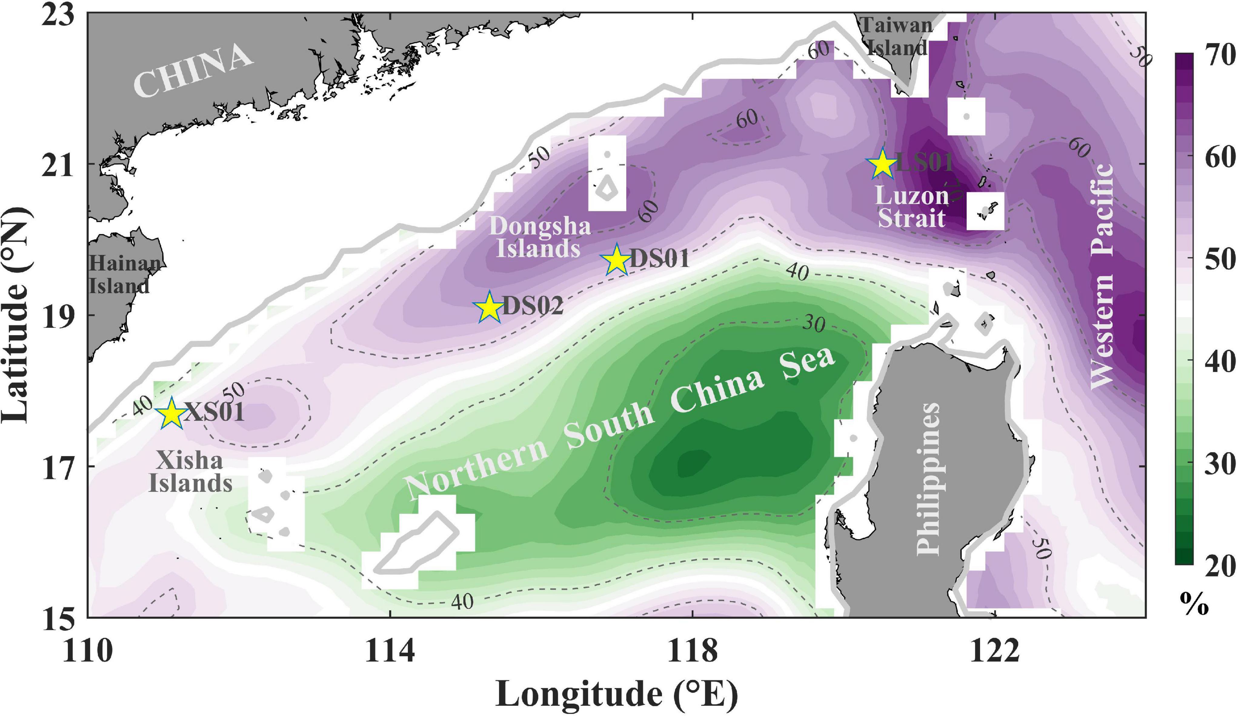
Figure 1. The annual mean of the ratios between the intraseasonal and raw sea level anomaly STD (1993–2019). Solid gray line: 200 m isobath; yellow stars: mooring stations.

TABLE 1

Table 1. Detailed mooring information.

Satellite Altimeter and Reanalysis Data

The SLA data from 1993 to 2019 were distributed by the Copernicus Marine Environment Monitoring Service. The daily gridded SLA has a horizontal resolution of 0.25° × 0.25° (Ducet et al., 2000). The data with the water depth shallower than 200 m were masked in this study.

An eddy detection scheme based on the geometry of velocity vector fields was used to identify the mesoscale eddies (Nencioli et al., 2010; Dong et al., 2012). The eddy center was defined as the location of the local minimum of the velocity fields, and the boundary was defined as the outermost closed streamline around the center, across which the velocity magnitudes were still increasing in the radial direction. In this study, the radius was the average distance from the center to the boundary, and the propagation speed was obtained by dividing the propagation distance by the time.

A Hybrid Coordinate Ocean Model (HYCOM) reanalysis product was used in this study. The HYCOM data have a time resolution of 1 day, a horizontal resolution of 1/12 × 1/12°, and 40 uneven vertical levels. The data in the upper 1,000 m from January 2003 to December 2012 were used for energy analysis. The reanalysis system assimilated available satellite altimeter observations, satellite sea surface temperature, and in situ data (Cummings and Smedstad, 2013).

Results

Generally Spatial Features of Intraseasonal Variability

The ratio of standard deviation (STD) of 10–110-day band-passed SLA to that of the raw SLA (i.e., STD of 10–110-day SLA/STD of raw SLA) is shown in Figure 1, demonstrating the contribution of ISV to the total variability. The ISV dominated the variability of SLA in the Luzon Strait and along the northern slope (Figure 1). It accounted for 25–70% (with an average value of ∼49%) of the total variability in the NSCS. In particular, ISV explained more than 50% of the total variability on the slope and ∼70% in the Luzon Strait. ISV weakened westward from the Luzon Strait to Xisha Islands.

The spatial features of the intraseasonal kinetic energy were revealed by the ADCP observed velocity fields. Here, we recorded the intraseasonal kinetic energy as the eddy kinetic energy (EKE) calculated as EKE = 1/2 (u′² + v′²), where u′ and v′ is 10–110-day band-passed zonal and meridional velocity anomaly, respectively. EKE decreased obviously with depth at LS01, DS01, and DS02. In the upper 150 m, it was even greater than 1,200 cm²/s² at some time, but almost weaker than 300 cm²/s² below 200 m (Figure 2). The vertical features of EKE at XS01 were different from those at the other three stations, exhibiting a non-significant change with depth that was usually lower than 300 cm²/s² throughout the upper layer (Figure 2). The enhanced EKE bursts at LS01, DS01, and DS02 were correlated with the time lags among them, indicating that the ISV propagated westward along the slope (Figure 2). However, the correlation was weak between XS01 and the other stations.

FIGURE 2

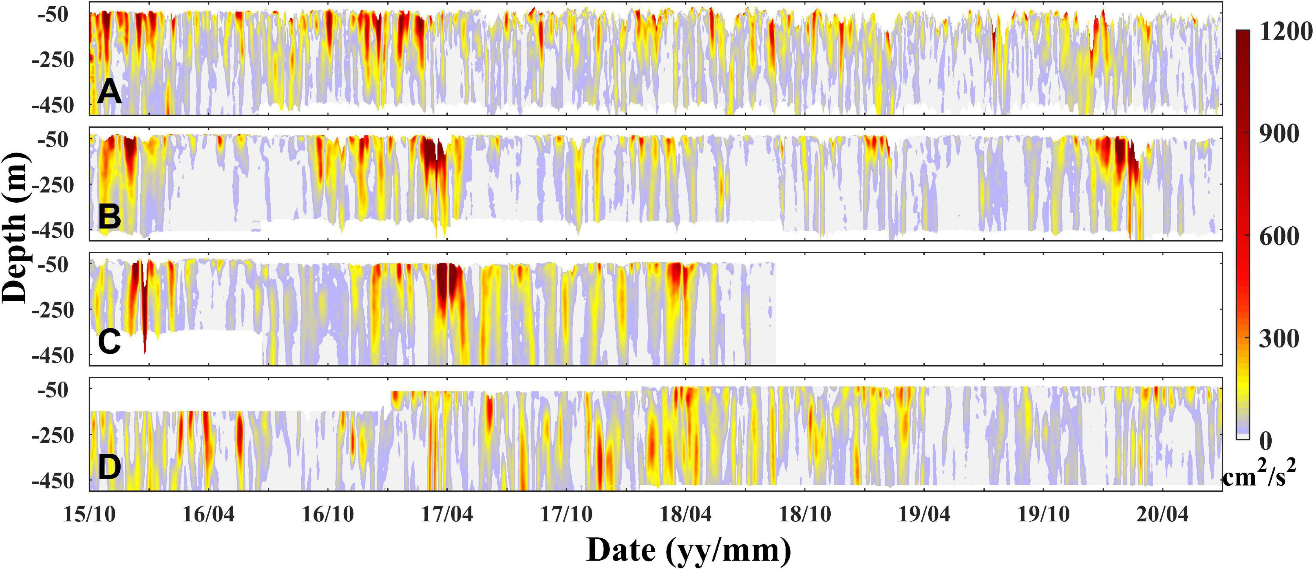
Figure 2. Time series of 10–110-day eddy kinetic energy (cm²/s²). Station (A) LS01, (B) DS01, (C) DS02, and (D) XS01.

The time-averaged EKE profiles at the four mooring sites are shown in Figure 3. EKEs exhibited a maximum value in the subsurface of ∼70 m at DS01 and DS02. The subsurface maximum EKE was consistent with the previous study of Wang et al. (2020a), who reported a subsurface (40–70 m) speed maximum existed in the NSCS, and it originated from the Kuroshio intrusion. The EKE decreased rapidly with depth at LS01, as did DS01 and DS02 below 70 m depth. However, the EKE was vertically aligned at XS01, with the vertical difference less than 40 cm²/s². In the upper 150 m, EKE at LS01, DS01, and DS02 was much greater than that at XS01, whereas it showed a slight difference below 200 m. EKE at XS01 even became the strongest below 320 m, significantly stronger than that at LS01 and DS01. The time- and vertical-averaged EKE was 77.3, 64.1, 91.6, and 61.2 cm²/s² at LS01, DS01, DS02, and XS01, respectively. The strongest ISV was observed at DS02, and the weakest ISV was observed at XS01. The relatively weak ISV at XS01 was possibly due to that Xisha Islands are located at the dissipation area of most mesoscale eddies in the NSCS (Chen et al., 2011; He et al., 2018).

FIGURE 3

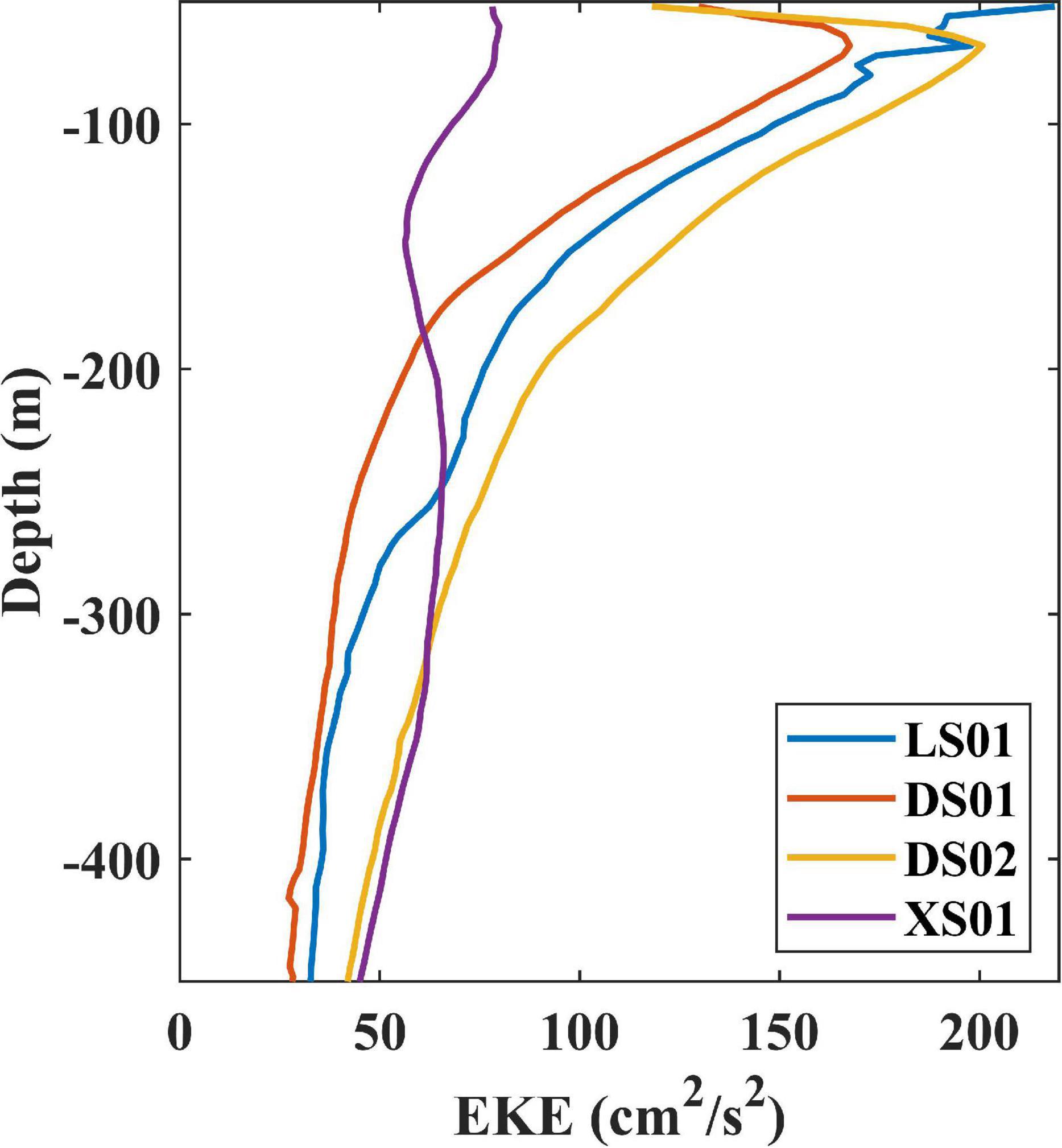
Figure 3. Vertical structure of time-averaged 10–110-day eddy kinetic energy (cm²/s²).

Spatial Differences Between the Two Main Frequency Bands of Intraseasonal Variability

We calculated the kinetic energy spectra in the variance-preserving form using the ADCP-observed velocity in each layer at the four mooring sites to examine the dominant frequency bands of the variability of the current (Figure 4). Notably, at DS02, the velocity between 350 and 450 m was only observed from July 2016 to August 2018 (Figure 2C), resulting in a break in the spectra at ∼350 m (Figure 4C). At XS01, there was no observation in the upper 150 m before January 2017 (Figure 2D). Thus, only data from January 2017 to July 2020 were used to calculate the spectrum.

FIGURE 4

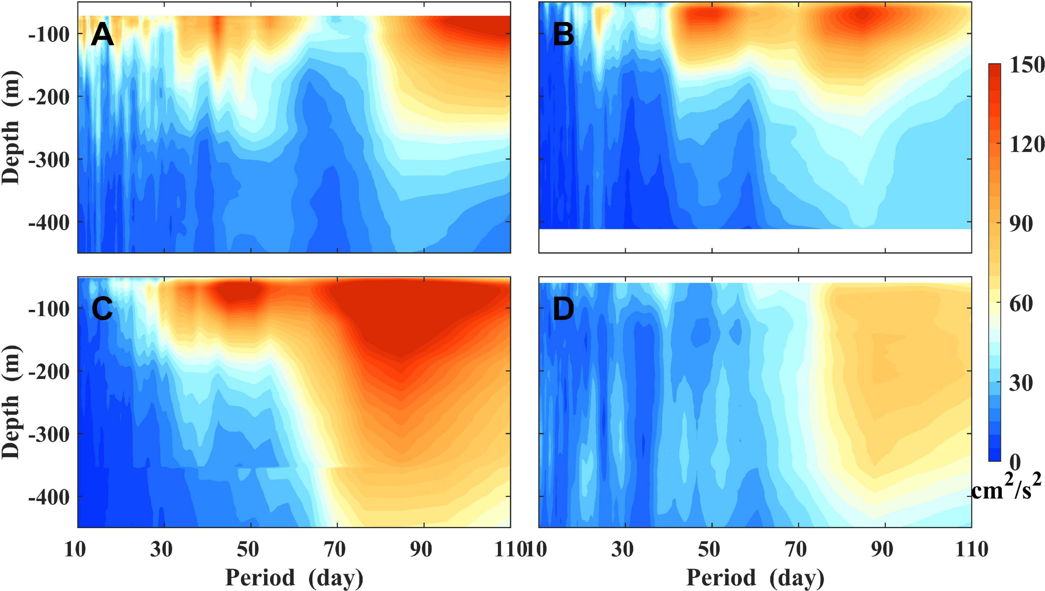
Figure 4. Kinetic energy spectra (cm²/s²) in variance-preserving form. Station (A) LS01, (B) DS01, (C) DS02, and (D) XS01. XS01 spectrum was calculated from 3.5 years of data (January 2017 to July 2020).

As shown in Figure 4, the spectra at the period of ∼65 days were weaker than those on both sides at LS01, DS01, and DS02. At each of the three mooring sites, there were two significant peak frequencies with the periods shorter and longer than 65 days. However, the spectrum of XS01 was strong only in the period longer than 65 days with a peak much weaker than that of the other three stations (Figure 4). The peak periods of the spectra were different at the four mooring sites. For the longer period ISV, the variance was strongest at the period of ∼85 days at DS01 and DS02 (Figures 4B,C); the peak period appeared at ∼108 and ∼90 days at LS01 and XS01, respectively (Figures 4A,D). For the shorter period ISV, the peak period was ∼45 days at LS01, DS01, and DS02. Additionally, the spectrum with the period of 10–30 days was slightly strong in the upper 200 m at LS01, while it was weak at the other three stations. It demonstrated that the high-frequency ISV in the upper 200 m was stronger at LS01 than that at other stations. The large variances of the kinetic energy spectra with the period of 10–65 days mainly appeared in the upper 200 m at LS01, DS01, and DS02, and they decreased rapidly with depth (Figures 4A–C). Below 200 m, the variances in the longer period (65–110 days) ISV were larger than that in the shorter period (10–65 days), suggesting that the low-frequency ISV had a deeper influence and the high-frequency ISV mainly concentrated on the upper layer (Figure 4).

Kinetic energy spectra analysis revealed differences between ISV periods shorter and longer than 65 days at the four mooring sites. Therefore, we divided ISV into two frequency bands, a high-frequency with a period of 10–65 days and a low-frequency with a period of 65–110 days. Similar to the vertical distribution of the kinetic energy spectra, the 10–65-day EKE weakened rapidly with depth at LS01, DS01, and DS02 (Figures 5A–C). The high-frequency ISV was weakest at XS01 (Figure 5D). The low-frequency EKE was generally weaker than the high-frequency EKE at all the four mooring sites (Figures 5, 6). Both the low- and high-frequency ISV presented a westward propagation characteristic. The low-frequency ISV could propagate westward from LS01 to XS01 (Figure 6), whereas the high-frequency ISV just propagated to DS02. The high-frequency ISV at XS01 showed no significant relationship with that at the other three mooring sites (Figure 5).

FIGURE 5

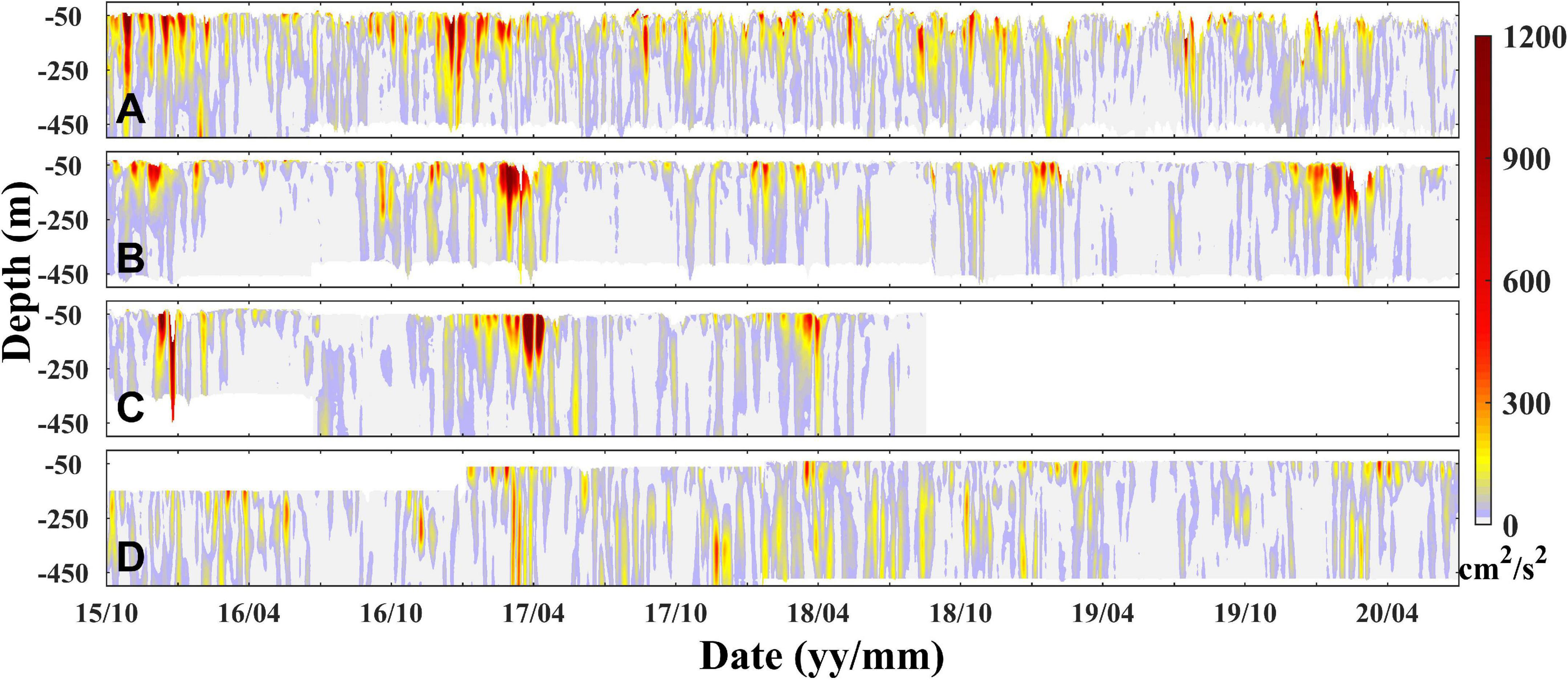
Figure 5. Time series of 10–65-day eddy kinetic energy (cm²/s²). Station (A) LS01, (B) DS01, (C) DS02, and (D) XS01.

FIGURE 6

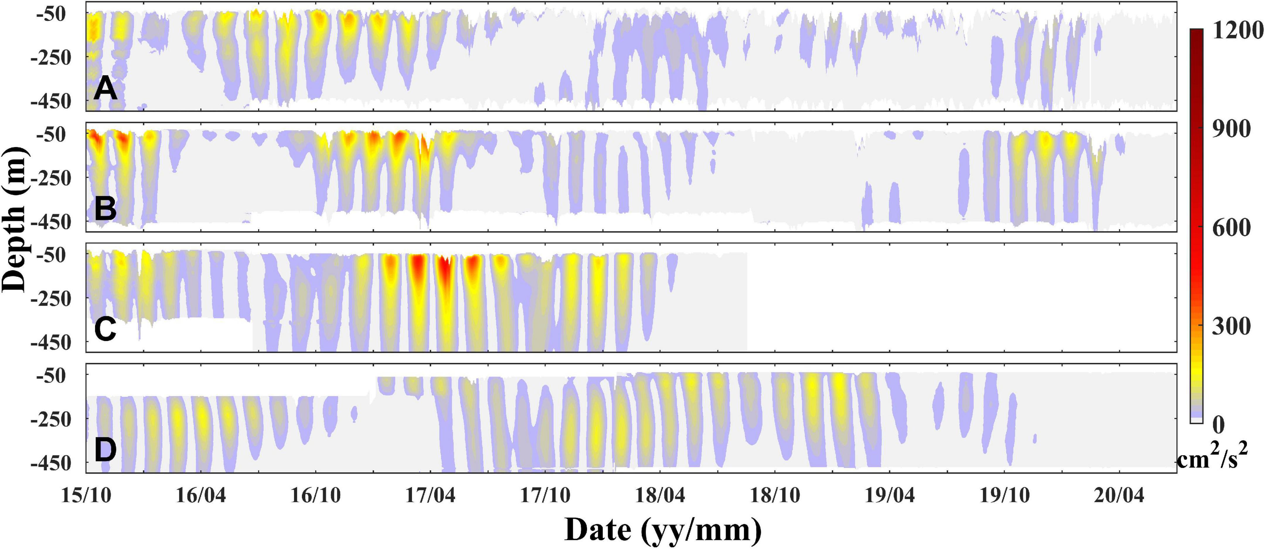
Figure 6. Time series of 65–110-day eddy kinetic energy (cm²/s²). Station (A) LS01, (B) DS01, (C) DS02, and (D) XS01.

The time-averaged EKE profiles with periods 10–65 days and 65–110 days are shown in Figure 7. Both the high- and low-frequency EKE exhibited a subsurface maximum characteristic at DS01 and DS02, with an additional occurrence at LS01 for the low-frequency (Figure 7). The high-frequency EKE decreased quickly below 70 m at LS01, DS01, and DS02 (Figure 7A). However, the vertical distribution of EKE showed that the low-frequency ISV had less variations with depth at the four mooring sites (Figure 7B). The high-frequency EKE weakened westward from LS01 to XS01 (Figure 7A), with mean values of 56.5, 36.3, 44.5, and 34.7 cm²/s² at LS01, DS01, DS02, and XS01, respectively (Table 2). However, the low-frequency EKE was strongest at DS02 with the mean value of 49.4 cm²/s² and weakest at LS01 with the mean value of 22.5 cm²/s² (Figure 7 and Table 2). Thus, the ISV was strongest at DS02 (with a time- and vertical-averaged EKE of 91.6 cm²/s²) among the four mooring sites (Figure 3 and Table 2).

FIGURE 7

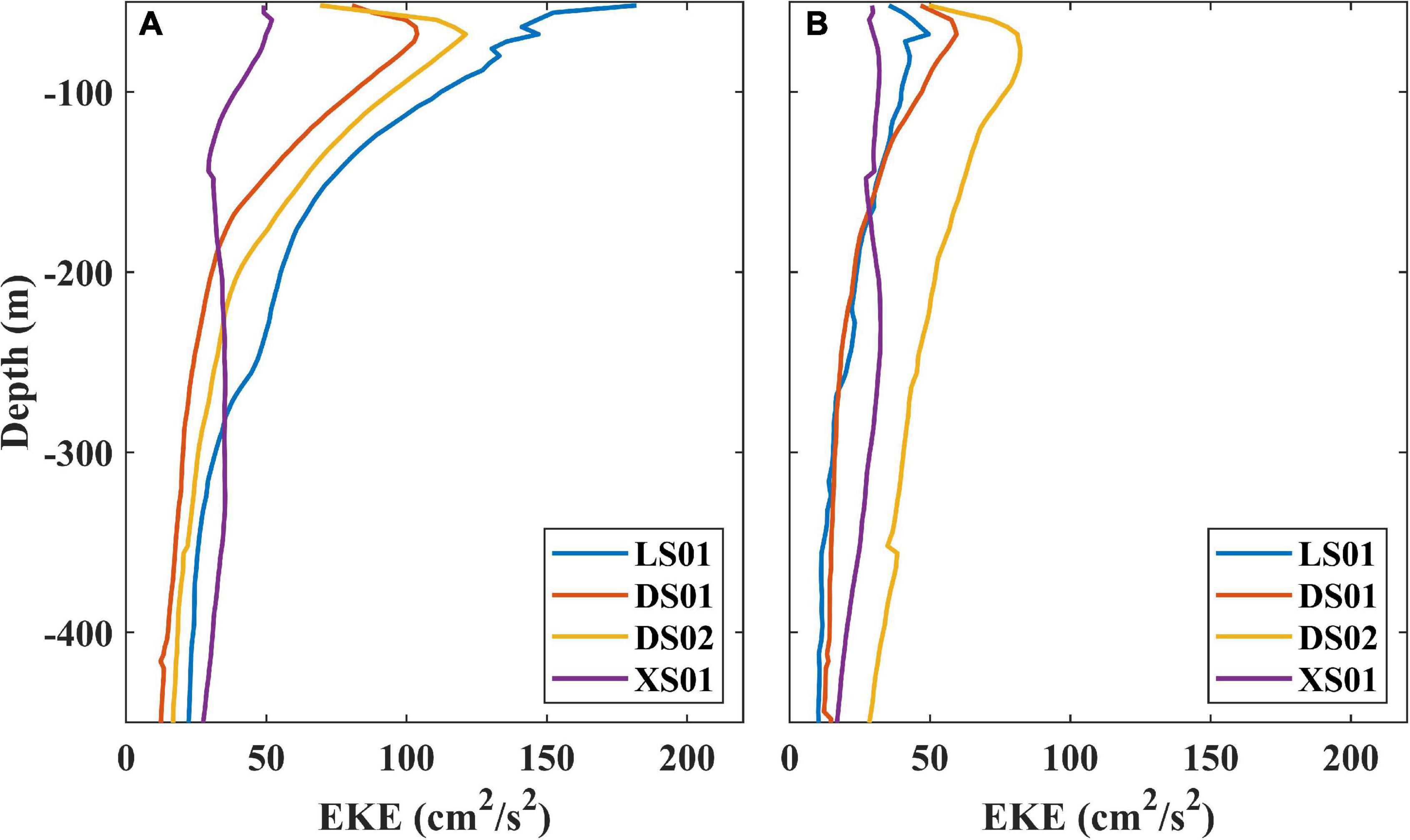
Figure 7. Vertical structure of time-averaged eddy kinetic energy (cm²/s²) at the period of (A) 10–65 days and (B) 65–110 days.

TABLE 2

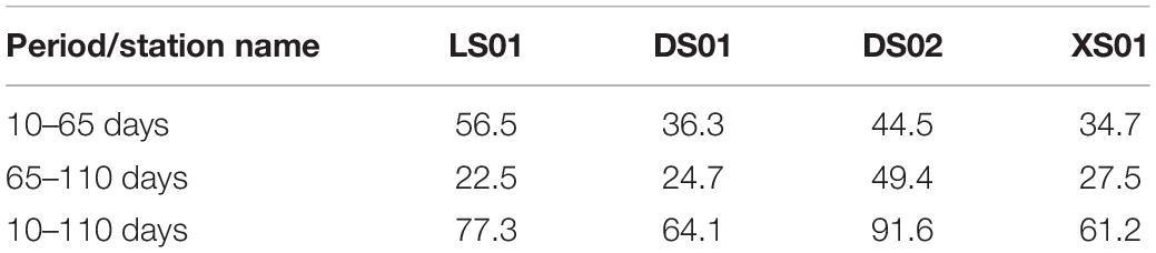
Table 2. Time- and vertical-averaged eddy kinetic energy of three periods (cm²/s²).

To investigate the horizontal distribution, the annual mean standard deviation of intraseasonal SLA (hereinafter, STD SLA) in the two periods (10–65 days and 65–110 days) in the NSCS are shown in Figures 8A,B. We obtained the STD SLA by calculating the standard deviation of band-passed SLA in each year and then taking the average of the standard deviations from 1993 to 2019. The horizontal distribution of STD SLA in the two periods exhibited obviously different patterns. For the 10–65-day ISV, the STD SLA was high in the Luzon Strait, connecting the NSCS and the western Pacific and then forming a continuous high STD SLA band (Figure 8A). There was a high core in the southwest Taiwan Strait at around 118.8°E, 21.3°N. The STD SLA decreased rapidly along the slope, which declined to below 3 cm in the west of 115°E (Figure 8A). For 65–110-day ISV, the STD SLA was quite low in the Luzon Strait compared with both sides of the strait, forming a gap between the NSCS and the western Pacific (Figure 8B). However, the STD SLA maintained relatively high along the slope from 111 to 120°E and had two high cores. One was near the DS02, which can explain why the 65–110-day kinetic energy was so strong at this station (Figure 7B and Table 2). The other was at almost the same position as the high core of 10–65-day ISV. The high-frequency ISV of SLA at LS01 was much stronger than the low-frequency ISV, but the opposite at DS02. The two frequency band signals had almost equal strength at DS01. At XS01, the high-frequency ISV was slightly stronger than the low-frequency ISV. These results were consistent with the spatial features of mooring observed EKE and spectrum analysis.

FIGURE 8

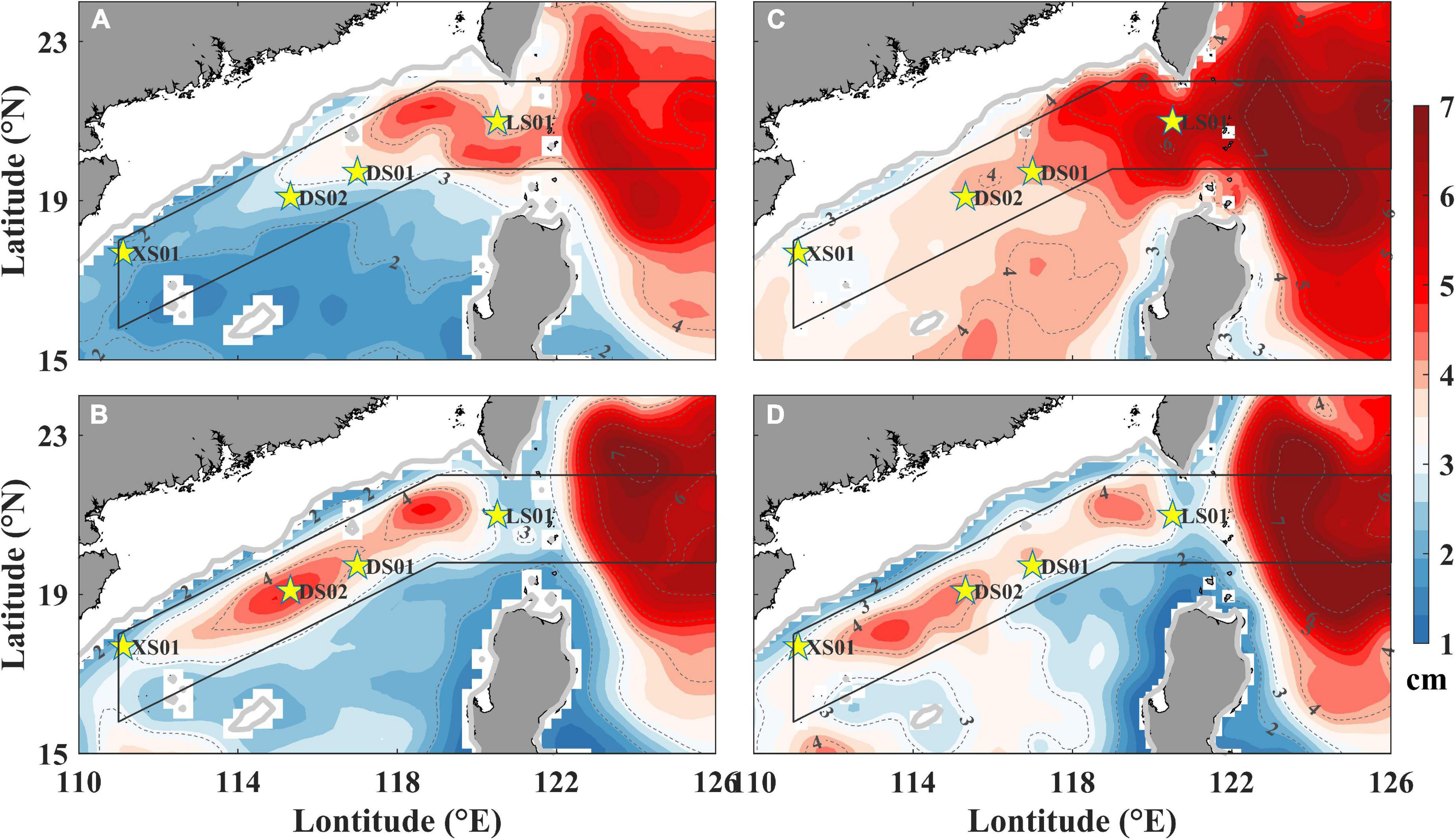
Figure 8. The annual mean standard deviation of intraseasonal sea level anomaly (SLA, cm) and sea surface height (SSH, cm) of the two periods derived from AVISO (HYCOM). (A) 10–65-day SLA; (B) 65–110-day SLA; (C) 10–65-day SSH; (D) 65–110-day SSH. Solid gray line: 200 m isobath; yellow stars: mooring stations.

The spatial distribution of ISV could be well reproduced by the sea surface height (SSH) from HYCOM (Figures 8C,D), confirming the existence of the spatial differences between the two frequency bands. The general spatial features of ISV calculated by HYCOM and AVISO were highly similar in the Luzon Strait and the northern slope. The slight differences were that the high core of 10–65-day ISV appeared at the Luzon Strait (120.3°E, 20.4°N), and the strength of 10–65-day ISV became stronger than that of 65–110-day ISV on the whole. The reproduction of spatial distribution of ISV enabled us to use HYCOM data to do energy analysis later.

Figure 9 shows the multi-year mean intraseasonal SLA along with the high STD SLA band from 111 to 126°E. The intraseasonal SLAs displayed distinct wave-like signals alternated between positive and negative for both frequency bands. The alternation of positive and negative SLA signals is associated with the mesoscale eddies (Wang et al., 2018). The 10–65-day ISV can propagate westward from the western Pacific to the NSCS for most of the time (Figure 9A). However, the 65–110-day ISV seemed to hardly propagate into the NSCS directly, which was weak in the Luzon Strait (120–122°E, Figure 9B). The significant gap in the Luzon Strait was also identical to the horizontal distribution of the STD SLA (Figures 8B,D). The propagation speed in the NSCS was ∼0.13 m/s for 10–65-day ISV and ∼0.10 m/s for 65–110-day ISV. In the western Pacific (122–126°E), it was ∼0.20 m/s for 10–65-day ISV and ∼0.10 m/s for 65–110-day ISV. Thus, the propagation speed of high-frequency ISV was faster than that of low-frequency ISV in the NSCS. The propagation speed of high-frequency ISV in the NSCS was much slower than that in the western Pacific. However, the propagation speed of low-frequency ISV varied slightly between the two sides of the Luzon Strait.

FIGURE 9

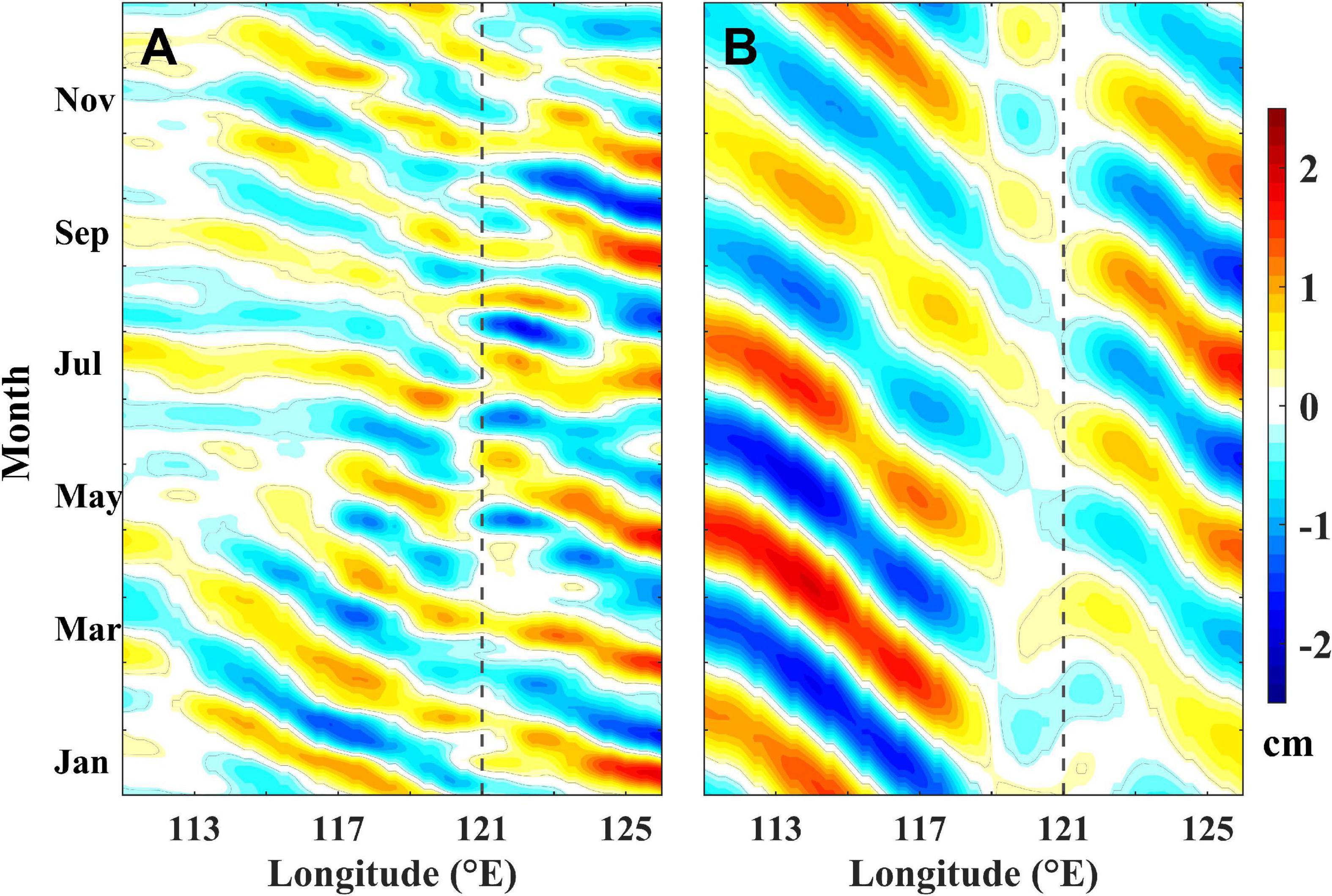
Figure 9. Hovmöller diagrams of annual mean sea level anomaly (cm) of two periods along with the black box of Figure 8. (A) 10–65-day period; (B) 65–110-day period. Black dashed lines: central Luzon Strait.

Energy Transfer Governing the Two Main Intraseasonal Variability Frequency Bands

Energy analysis was conducted to explore the dynamic processes resulting in the spatial differences between the two frequency bands of ISV. EKE and eddy available potential energy (EPE) per unit mass is defined as follows (Böning and Budich, 1992):

$$\text{EKE}={\displaystyle \frac{1}{2}}\left(u^{{}^{\prime }2}+v^{{}^{\prime }2}\right),$$

$$\text{EPE}=-{\displaystyle \frac{g{\tilde{\mathrm{\rho }}}^{{}^{\prime }2}}{2\mathrm{\rho }\left(\partial {\overline{\mathrm{\rho }}}_{\mathrm{\theta }}/\partial z\right)}}.$$

Here, g is the gravitational acceleration, $\tilde{\mathrm{\rho }}(x,y,z,t)=\mathrm{\rho }(x,y,z,t)-{\mathrm{\rho }}_b(z)$, ρ_b(z) is the depth-dependent background density, which is the temporal mean from January 2003 to December 2012 and the horizontal mean over the domain shown in Figure 8. ${\overline{\mathrm{\rho }}}_{\mathrm{\theta }}(z)$ is the temporal and horizontal mean potential density. The transient components of velocity and density are defined as the band-passed variabilities of 10–65 days and 65–110 days. The residual low-frequency variabilities (with periods > 65 days and > 110 days) are treated as the background state.

The four-box energy diagram illustrates the energy transfer between mean and eddy kinetic and potential energies (Lorenz, 1955; Böning and Budich, 1992; Beckmann et al., 1994). This method has been widely applied to calculate instabilities caused by eddy-mean flow interaction in the SCS (Zhuang et al., 2010; Zu et al., 2013; Geng et al., 2016). The eddy-mean flow interaction terms are defined as follows:

$$T_2=-{\displaystyle \frac{g}{-\mathrm{\rho }\left(\partial {\overline{\mathrm{\rho }}}_{\mathrm{\theta }}/\partial z\right)}}\left(u^{\prime }{\tilde{\mathrm{\rho }}}^{\prime }{\displaystyle \frac{\partial \overline{\tilde{\mathrm{\rho }}}}{\partial x}}+v^{\prime }{\tilde{\mathrm{\rho }}}^{\prime }{\displaystyle \frac{\partial \overline{\tilde{\mathrm{\rho }}}}{\partial y}}\right),$$

$$T_4=-\left(u^{\prime }{u}^{\prime }{\displaystyle \frac{\partial \overline{u}}{\partial x}}+u^{\prime }{v}^{\prime }\left({\displaystyle \frac{\partial \overline{v}}{\partial x}}+{\displaystyle \frac{\partial \overline{u}}{\partial y}}\right)+v^{\prime }{v}^{\prime }{\displaystyle \frac{\partial \overline{v}}{\partial y}}\right).$$

Here, T₂ is the conversion between mean potential energy (MPE) and EPE. Positive values of T₂ correspond to baroclinic instability (BCI) due to the intense density differences between the eddy and mean flow, indicating that the MPE is converted to EPE. T₄ is the work of the Reynolds stresses against the mean shear. Positive values of T₄ imply barotropic instability (BTI) due to strong velocity shear, indicating that the mean kinetic energy (MKE) is converted to EKE.

The horizontal distributions of vertically integrated EKE and EPE in the two frequency bands showed similar spatial patterns with the STD SLA, especially for the EPE (Figures 8, 10). The energy of 10–65 days was stronger than that of 65–110 days, but this difference was relatively weak for EPE, and EPE was stronger than EKE for both periods. These results suggested that EPE was more closely related to the spatial differences between the two frequency bands.

FIGURE 10

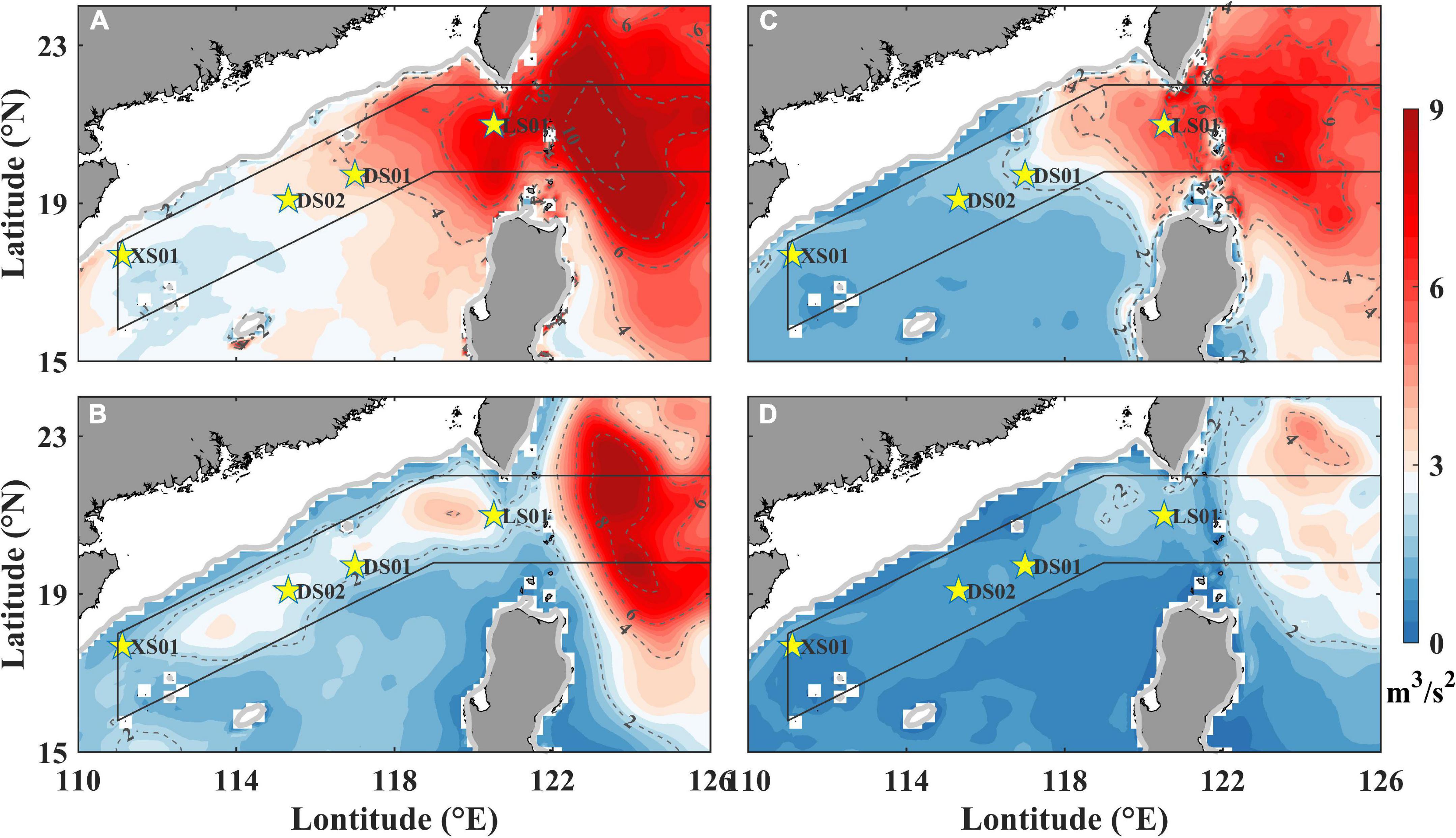
Figure 10. Horizontal distribution of vertical integrated energy. (A) Eddy potential energy (EPE) in 10–65-day period (m³/s²); (B) EPE in 65–110-day period (m³/s²); (C) Eddy kinetic energy (EKE) in 10–65-day period (m³/s²); and (D) EKE in 65–110-day period (m³/s²) averaged from January 2003 to December 2012.

Figure 11 shows the vertical integration of T₂ and T₄ averaged from January 2003 to December 2012, where only positive values were considered. The sum of T₂ and T₄ in the two frequency bands presented similar spatial patterns with the ISV in two main frequency bands, except for the 65–110-day ISV in the Luzon Strait (Figures 8, 11). The sums of T₂ and T₄ in the two frequency bands showed strong BCI and BTI in the Luzon Strait and its western part. Individually, strong T₂ and T₄ in 10–65 days were mainly concentrated on the Luzon Strait and weakened westward along the slope. T₂ and T₄ in 65–110 days were relatively strong on the slope of the NSCS. The instabilities mainly occurred in the Luzon Strait and the northern slope of the SCS (Figure 11), suggesting that much energy was converted from the large-scale current to the intraseasonal-scale current there (Zhang et al., 2015). Thus, the instabilities in the two intraseasonal scales could result in different spatial patterns of ISV in the two frequency bands.

FIGURE 11

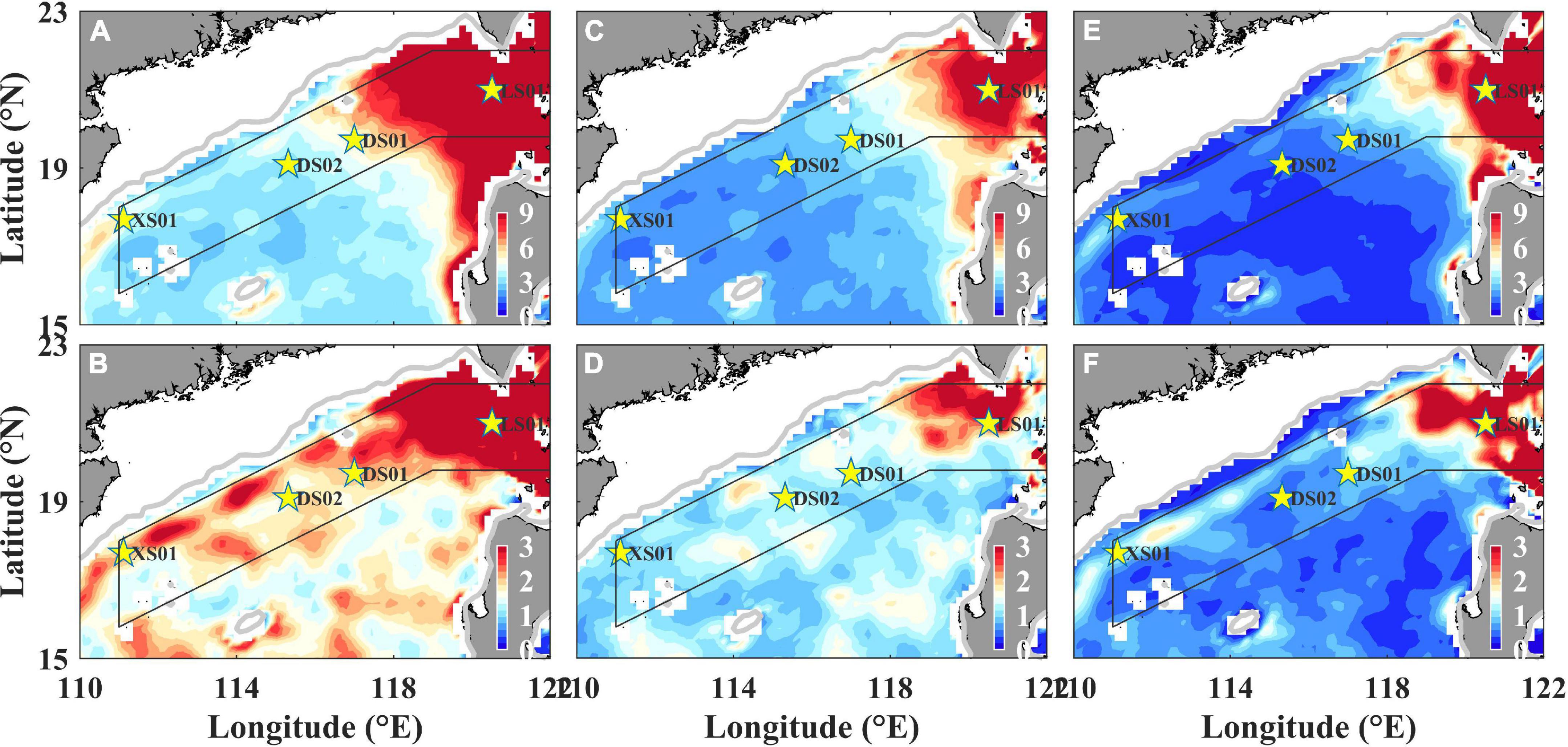
Figure 11. Horizontal distribution of vertical integrated T₂ and T₄. (A) Sum of T₂ and T₄ in 10–65-day period (×10^–6 m³/s³); (B) sum of T₂ and T₄ in 65–110-day period (×10^–6 m³/s³); (C) T₂ in 10–65-day period (×10^–6 m³/s³); (D) T₂ in 65–110-day period (×10^–6 m³/s³); (E) T₄ in 10–65-day period (×10^–6 m³/s³); and (F) T₄ in 65–110-day period (×10^–6 m³/s³) averaged from January 2003 to December 2012 (only positive values considered).

Discussion

Intraseasonal Variability and Mesoscale Eddies

Intraseasonal variability is closely associated with the activity of mesoscale eddies in the NSCS (Liu et al., 2001; Zhuang et al., 2010; Wang et al., 2020b). Figure 12 shows the mean radius and propagation speed of mesoscale eddies from 1993 to 2019, which were located in the black box shown in Figure 8. The mean eddy radius in the NSCS and the western Pacific was significantly higher than that in the Luzon Strait. The radius gradually increased along the slope from 121°E westward up to ∼115°E (the position of one high core of the low-frequency ISV in Figure 8B), reaching its maximum. The spatial features of eddy propagation speed were almost opposite to that of eddy radius. The mean eddy propagation speed in the NSCS and the western Pacific was slower than that in the Luzon Strait. Notably, the eddy propagation speed in the western Pacific was faster than that in the NSCS, which was identical to the propagation speed of the 10–65-day ISV in Figure 9. The eddy propagation speed showed a decreasing trend from 121°E to the west, though it was slightly slow at ∼119°E, possibly because many mesoscale eddies dissipate here due to the topography of the Dongsha Islands. The propagation speed was stable from 115 to 111°E. Compared with the spatial features of the two frequency bands of SLA (Figures 8A,B), it can be found that the high-frequency ISV was strong when the eddy radius was small and the eddy propagation speed was fast, and low-frequency ISV was strong when the eddy radius was large, and the eddy propagation speed was slow. Therefore, the eddy radius was inversely proportional to the strength of the high-frequency ISV, and it was directly proportional to the strength of the low-frequency ISV. This proportional relationship was reversed for the eddy propagation speed.

FIGURE 12

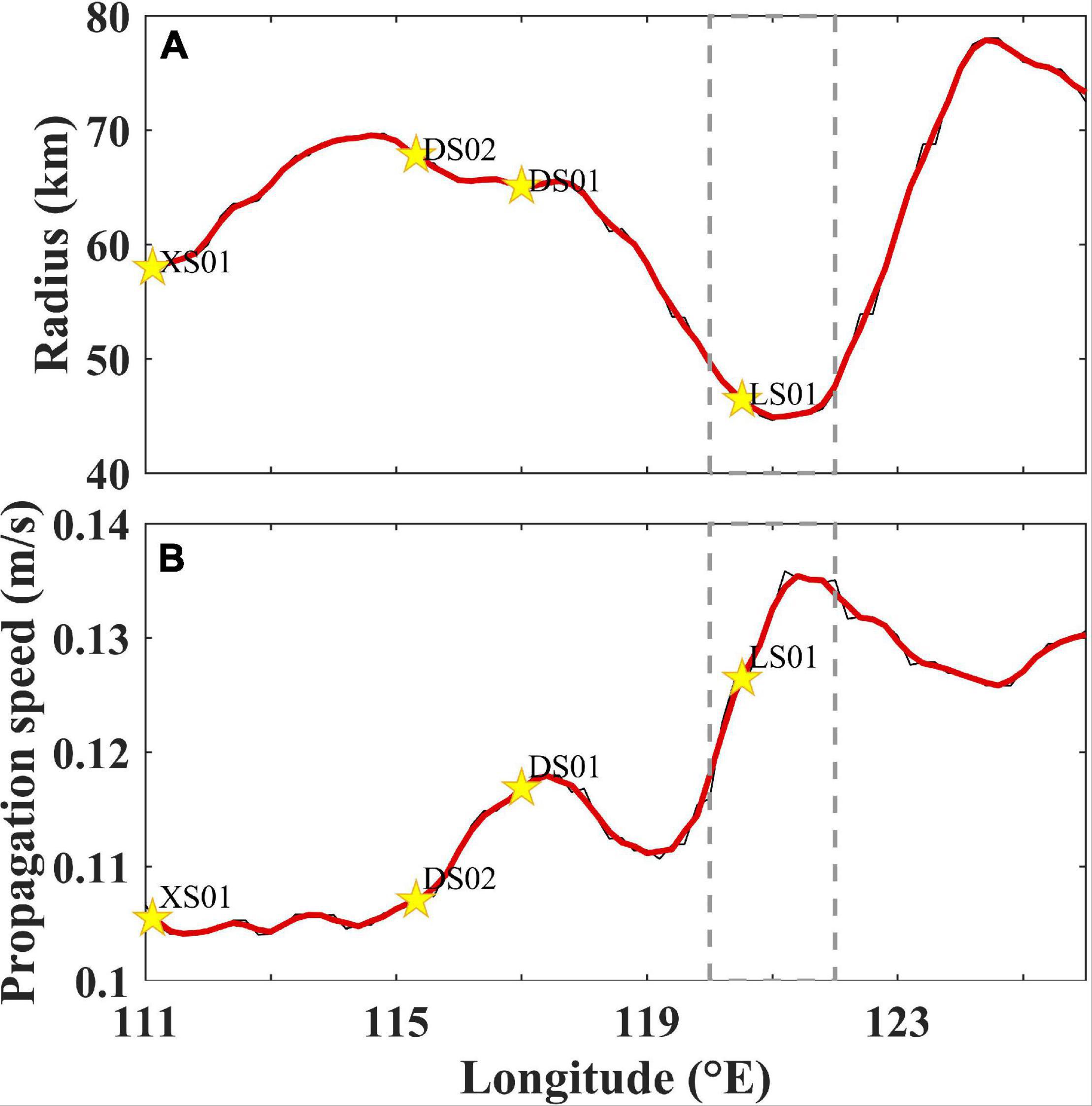
Figure 12. (A) Mean eddy radius (km) and (B) mean eddy propagation speed (m/s) along with the black box of Figure 8. Thin black lines: raw data; thick red lines: running means of raw data; mooring stations (yellow stars) are marked on lines according to longitudes; gray dashed boxes: Luzon Strait.

We used the mean eddy radius of ∼60 km as the size threshold to distinguish the eddies. Figure 13 shows the spatial distribution of the number of mesoscale eddies in the two ranges of eddy radius. The majority of eddies with a radius < 60 km was located in the Luzon Strait and its west side, although there were several near the Xisha Islands. Eddies > 60 km were mostly distributed along the slope, but few in the Luzon Strait. The spatial distributions of mesoscale eddies in the two sizes were similar to the spatial distributions of ISV in two dominant frequency bands (Figure 8).

FIGURE 13

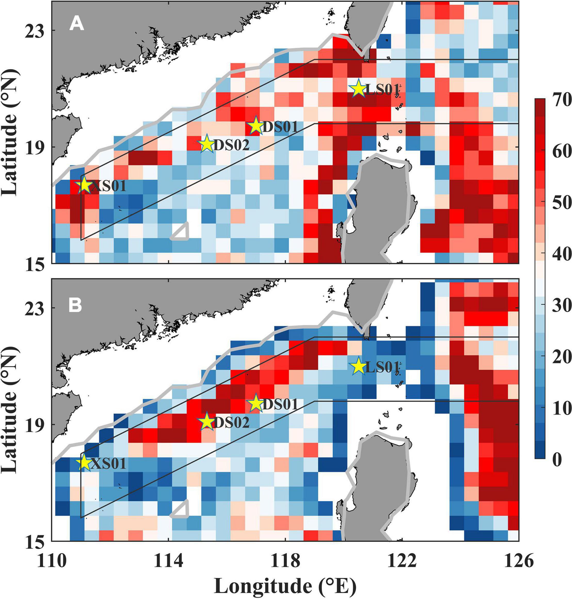
Figure 13. Spatial distribution of (A) the number of eddy radius smaller than 60 km and (B) the number of eddy radius larger than 60 km.

The relationship between the two frequency bands of ISV and the mesoscale eddies can be understood from the perspective of wave theory (i.e., frequency = wave speed/wavelength, $\mathrm{\sigma }=\frac{v}{\mathrm{\lambda }}$), if we consider that the eddy size corresponds to wavelength λ and the eddy propagation speed corresponds to wave speed v. Take the Luzon Strait as an example. The eddy propagation speed was fast and the eddy radius was small in the Luzon Strait, corresponding to a high value of v and a low value of λ. According to the formula, $\mathrm{\sigma }=\frac{v}{\mathrm{\lambda }}$, this will result in a high value of frequency σ, coinciding with our results that showed a strong high-frequency signal in the Luzon Strait (Figure 8A). For the remaining areas of the high STD SLA band, except for ∼119°E, the results fitted this condition. The eddy propagation speed was slightly slow at ∼119°E, probably because of the strength of the low-frequency signal. Therefore, the spatial differences of ISV in the two frequency bands may result from the spatial differences of eddy radius and propagation speed.

Effects of the Western Pacific

Intraseasonal variability in the NSCS was closely correlated with that of the western Pacific, especially the 10–65-day ISV (Figures 8, 9). Zheng et al. (2011) reported that the non-linear Rossby eddies (NREs) originating from the tropical Pacific propagate westward and at least 60% of them enter into the NSCS. Some observational studies further confirmed that the non-linear Rossby eddies penetrate the Luzon Strait from the Pacific to the NSCS (Hu et al., 2012). The 10–65-day ISV, whose strength was inversely proportional to eddy radius, can frequently propagate westward from the Pacific directly to the NSCS. It demonstrates that the waves with short wavelengths can penetrate the Luzon Strait from the Pacific to the SCS directly.

Some investigators suggested that ISV in the NSCS is not from the western Pacific; rather, the ISV is locally generated just west of Luzon Strait and then propagates southwestward (Wu and Chiang, 2007; Zhuang et al., 2010). This viewpoint is coincident that the 65–110-day ISV cannot propagate from the Pacific into the NSCS directly (Figure 9B). The 65–110-day ISV was quite weak (approaching zero) at ∼121°E in the Luzon Strait. However, the 65–110-day ISV presented high similarity on both sides of the strait since the propagation speed, the strength of ISV, and time lagging were linked between the western Pacific and the NSCS (Figure 9B). We hypothesized that the indirect connection was realized as wave diffraction through a small hole, Luzon Strait. Obvious wave diffraction occurs on the premise that the hole size is smaller than or close to the wavelength. In our case, the Luzon Strait played the role of a small hole. Wave diffraction was more likely to occur for 65–110-day ISV with a large wavelength. So, although the 65–110-day ISV was weak at the Luzon Strait, we believe that the energy of 65–110-day ISV in the NSCS was partly from the western Pacific and then was maintained or strengthened by the BCI and BTI. It should be noted that the ISV in the upper circulation usually has two comparable origins: the dynamical instabilities of the background flow and the intraseasonal wind forcing (Wang et al., 2016). This study mainly investigates the internal component of the ocean associated with eddy generation. The wind stress curls could also spin up cyclonic and anticyclonic eddies in the SCS (Wang et al., 2007). Yang et al. (2017) found that the intraseasonal wind results in the ISV of sea surface height in summer in the southeast of Vietnam. The relative contribution of dynamical instabilities of the background flow and the intraseasonal wind forcing to the ISV in the SCS needs to be further studied.

Conclusion

Based on four long-time mooring observations and satellite observations, a prominent ISV had been found in the NSCS, especially in the Luzon Strait and the northern slope with the ISV contributing more than 50% of the total variability. The ISV in the NSCS consisted of two dominant frequency bands, 10–65 days and 65–110 days, corresponding to high-frequency and low-frequency signals of ISV, respectively. The spatial features of the two frequency bands were quite different. The 10–65-day ISV was strong in the Luzon Strait and then weakened rapidly along the northern slope. The 65–110-day ISV was weak in the Luzon Strait, whereas it was relatively strong along the entire slope and had two high cores. One high core of the low-frequency ISV was near the Dongsha Islands, and the other was near southwestern Taiwan, where the high-frequency ISV was also strong. In addition, the two frequency bands exhibited a westward propagation characteristic along the northern slope. Vertically, the 10–65-day ISV decreased rapidly with depth at LS01 but was aligned at XS01. It exhibited a subsurface maximum at ∼70 m at DS01 and DS02 and then decreased quickly below 70 m. However, the 65–110-day ISV did not change much with depth at all four stations.

The 10–65-day ISV is likely to originate from the western Pacific, which can penetrate the Luzon Strait directly and propagate into the NSCS. However, the 65–110-day ISV could not propagate into the NSCS from the western Pacific directly, which seemed to have an indirect link between the western Pacific and the NSCS, maybe in a form similar to the wave diffraction due to the large wavelength of the low-frequency ISV. Furthermore, Hovmöller diagrams exhibited that the propagation speed of high-frequency ISV was faster than that of low-frequency ISV in the NSCS. The ISV was maintained or strengthened by the BCI and BTI after propagating from the western Pacific into the NSCS. BCI and BTI in the two intraseasonal scales resulted in the spatial differences of ISV between the two frequency bands.

The spatial distribution of ISV in the NSCS was closely associated with the radius and propagation speed of mesoscale eddies. The strength of high-frequency ISV was inversely proportional to the mean eddy radius, whereas the strength of low-frequency ISV was directly proportional to the mean eddy radius. This proportional relationship was reversed for eddy propagation speed. Moreover, the spatial distributions of mesoscale eddies in the two sizes were similar to that of the ISV in the two frequency bands. Further studies are needed to understand how the mesoscale eddies result in the ISV and how the ISV signals propagate from the western Pacific to the NSCS.

Data Availability Statement

The original contributions presented in the study are included in the article/supplementary material, further inquiries can be directed to the corresponding author.

Author Contributions

YS designed the research and guided the study. WX analyzed the data. WX and YS wrote the first draft of the manuscript. DW and QX contributed to the interpretation of the results. JC and YH contributed to the collection of mooring data. All authors contributed to the discussion of data analysis and manuscript writing.

Funding

This work was supported by the National Natural Science Foundation of China (41776036, 41521005, 91958202, 42076019, 91858203, 41906017, and 42076026), the Chinese Academy of Sciences Foundation (CXJJ-19-C18), Key Special Project for Introduced Talents Team of Southern Marine Science and Engineering Guangdong Laboratory (Guangzhou) (GML2019ZD0304), and the Open Project Program of State Key Laboratory of Tropical Oceanography (project LTOZZ2001 and LTOZZ2102). The ADCP velocity fields were provided by the Network of Field Observation and Research Stations of the Chinese Academy of Sciences.

Conflict of Interest

The authors declare that the research was conducted in the absence of any commercial or financial relationships that could be construed as a potential conflict of interest.

Publisher’s Note

All claims expressed in this article are solely those of the authors and do not necessarily represent those of their affiliated organizations, or those of the publisher, the editors and the reviewers. Any product that may be evaluated in this article, or claim that may be made by its manufacturer, is not guaranteed or endorsed by the publisher.

Acknowledgments

This study was benefited from the freely available datasets: the altimeter dataset (https://resources.marine. copernicus.eu/product-detail/SEALEVEL_GLO_PHY_L4_REP_ OBSERVATIONS_008_047/INFORMATION) and HYCOM reanalysis product (http://apdrc.soest.hawaii.edu/data/data.php). The main data supporting the findings in this study are available on the MediaFire repository (https://www.mediafire.com/file/9f3y90tvw6hen6x/SupplementaryData_xw.zip/file).

References

Beckmann, A., Böning, C. W., Brügge, B., and Stammer, D. (1994). On the generation and role of eddy variability in the central North Atlantic Ocean. J. Geophys. Res. 99, 20381–20391. doi: 10.1029/94JC01654

CrossRef Full Text | Google Scholar

Böning, C. W., and Budich, R. G. (1992). Eddy dynamics in a primitive equation model: sensitivity to horizontal resolution and friction. J. Phys. Oceanogr. 22, 361–381.

Google Scholar

Chen, G., Gan, J., Xie, Q., Chu, X., Wang, D., and Hou, Y. (2012). Eddy heat and salt transports in the South China Sea and their seasonal modulations. J. Geophys. Res. 117:C05021. doi: 10.1029/2011JC007724

CrossRef Full Text | Google Scholar

Chen, G., Hou, Y., and Chu, X. (2011). Mesoscale eddies in the South China Sea: mean properties, spatiotemporal variability, and impact on thermohaline structure. J. Geophys. Res. 116:C06018. doi: 10.1029/2010JC006716

CrossRef Full Text | Google Scholar

Chen, X., Qiu, B., Cheng, X., Qi, Y., and Du, Y. (2015). Intra-seasonal variability of pacific-origin sea level anomalies around the Philippine Archipelago. J. Oceanogr. 71, 239–249. doi: 10.1007/s10872-015-0281-9

CrossRef Full Text | Google Scholar

Cummings, J. A., and Smedstad, O. M. (2013). Variational Data Assimilation for the Global Ocean. In Data Assimilation for Atmospheric Oceanic and Hydrologic Applications Vol. II, Chap. 13. Berin: Springer, 303–343. doi: 10.1007/978-3-642-35088-7-13

CrossRef Full Text | Google Scholar

Dong, C., Lin, X., Liu, Y., Nencioli, F., Chao, Y., Guan, Y., et al. (2012). Three-dimensional oceanic eddy analysis in the Southern California Bight from a numerical product. J. Geophys. Res. 117:C00H14. doi: 10.1029/2011JC007354

CrossRef Full Text | Google Scholar

Ducet, N., Le Traon, P., and Reverdin, G. (2000). Global high-resolution mapping of ocean circulation from TOPEX/Poseidon and ERS-1 and -2. J. Geophys. Res. 105, 19477–19498. doi: 10.1029/2000JC900063

CrossRef Full Text | Google Scholar

Gan, J., Li, H., Curchitser, E. N., and Haidvogel, D. B. (2006). Modeling South China Sea circulation: response to seasonal forcing regimes. J. Geophys. Res. 111:C06034. doi: 10.1029/2005JC003298

CrossRef Full Text | Google Scholar

Gan, J., Liu, Z., and Hui, C. R. (2016). A three-layer alternating spinning circulation in the South China Sea. J. Phys. Oceanogr. 46, 2309–2315. doi: 10.1175/JPO-D-16-0044.1

CrossRef Full Text | Google Scholar

Geng, W., Xie, Q., Chen, G., Zu, T., and Wang, D. (2016). Numerical study on the eddy–mean flow interaction between a cyclonic eddy and Kuroshio. J. Oceanogr. 72, 1–19. doi: 10.1007/s10872-016-0366-0

CrossRef Full Text | Google Scholar

He, Q., Zhan, H., Cai, S., He, Y., Huang, G., and Zhan, W. (2018). A new assessment of mesoscale eddies in the South China Sea: surface features, three-dimensional structures, and thermohaline transports. J. Geophys. Res. 123, 4906–4929. doi: 10.1029/2018JC014054

CrossRef Full Text | Google Scholar

Hu, J., Kawamura, H., Hong, H., and Qi, Y. (2000). A review on the currents in the South China Sea: seasonal circulation, South China Sea warm current and kuroshio intrusion. J. Oceanogr. 56, 607–624. doi: 10.1023/A:1011117531252

CrossRef Full Text | Google Scholar

Hu, J., Zheng, Q., Sun, Z., and Tai, C. K. (2012). Penetration of nonlinear Rossby eddies into South China Sea evidenced by cruise data. J. Geophys. Res. 117:C03010. doi: 10.1029/2011JC007525

CrossRef Full Text | Google Scholar

Isoguchi, O., and Kawamura, H. (2006). MJO-related summer cooling and phytoplankton blooms in the South China Sea. Geophys. Res. Lett. 33:L16615. doi: 10.1029/2006GL027046

CrossRef Full Text | Google Scholar

Li, L., Nowlin, W. D., and Su, J. (1998). Anticyclonic rings from the Kuroshio in the South China Sea. Deep Sea Res. Part I Oceanogr. Res. Pap. 45, 1469–1482. doi: 10.1016/S0967-0637(98)00026-0

CrossRef Full Text | Google Scholar

Liang, Z., Xie, Q., Zeng, L., and Wang, D. (2018). Role of wind forcing and eddy activity in the intraseasonal variability of the barrier layer in the South China Sea. Ocean Dyn. 68, 363–375. doi: 10.1007/s10236-018-1137-9

CrossRef Full Text | Google Scholar

Liu, Q., Jia, Y., Liu, P., Wang, Q., and Chu, P. C. (2001). Seasonal and intraseasonal thermocline variability in the central South China Sea. Geophys. Res. Lett. 28, 4467–4470.

Google Scholar

Lorenz, E. N. (1955). Available potential energy and the maintenance of the general circulation. Tellus 7, 157–167. doi: 10.1111/j.2153-3490.1955.tb01148.x

CrossRef Full Text | Google Scholar

Nencioli, F., Dong, C., Dickey, T., Washburn, L., and Mcwilliams, J. C. (2010). A vector geometry-based eddy detection algorithm and its application to a high-resolution numerical model product and high-frequency radar surface velocities in the Southern California Bight. J. Atmos. Ocean Tech. 27:564. doi: 10.1175/2009JTECHO725.1

CrossRef Full Text | Google Scholar

Qiu, C., Liang, H., Huang, Y., Mao, H., Yu, J., Wang, D., et al. (2020). Development of double cyclonic mesoscale eddies at around Xisha Islands observed by a ‘Sea-Whale 2000’ autonomous underwater vehicle. Appl. Ocean Res. 101:102270. doi: 10.1016/j.apor.2020.102270

CrossRef Full Text | Google Scholar

Qu, T. (2000). Upper-layer circulation in the South China Sea. J. Phys. Oceanogr. 30, 1450–1460.

Google Scholar

Sheu, W. J., Wu, C. R., and Oey, L. Y. (2010). Blocking and westward passage of eddies in the Luzon Strait. Deep Sea Res. Part II Top. Stud. Oceanogr. 57, 1783–1791. doi: 10.1016/j.dsr2.2010.04.004

CrossRef Full Text | Google Scholar

Shu, Y., Chen, J., Li, S., Wang, Q., Yu, J., and Wang, D. (2019). Field-observation for an anticyclonic mesoscale eddy consisted of twelve gliders and sixty-two expendable probes in the northern South China Sea during summer 2017. Sci. China Earth Sci. 62, 451–458. doi: 10.1007/s11430-018-9239-0

CrossRef Full Text | Google Scholar

Shu, Y., Wang, Q., and Zu, T. (2018). Progress on shelf and slope circulation in the northern South China Sea. Sci. China Earth Sci. 61, 560–571. doi: 10.1007/s11430-017-9152-y

CrossRef Full Text | Google Scholar

Shu, Y., Xiu, P., Xue, H., Yao, J., and Yu, J. (2016). Glider-observed anticyclonic eddy in the northern South China Sea. Aquat. Ecosyst. Health. 19, 233–241. doi: 10.1080/14634988.2016.1208028

CrossRef Full Text | Google Scholar

Su, D., Lin, P., Mao, H., Wu, J., Liu, H., Cui, Y., et al. (2020). Features of slope intrusion mesoscale eddies in the northern South China Sea. J. Geophys. Res. 125:e2019JC015349. doi: 10.1029/2019JC015349

CrossRef Full Text | Google Scholar

Wang, F., Li, Y., and Wang, J. (2016). Intraseasonal variability of the surface zonal currents in the western tropical pacific ocean: characteristics and mechanisms. J. Phys. Oceanogr. 46, 3639–3660. doi: 10.1175/jpo-d-16-0033.1

CrossRef Full Text | Google Scholar

Wang, G., Chen, D., and Su, J. (2007). Winter eddy genesis in the eastern South China Sea due to orographic wind jets. J. Phys. Oceanogr. 38, 726–732. doi: 10.1175/2007JPO3868.1

CrossRef Full Text | Google Scholar

Wang, G., Su, J., and Chu, P. C. (2003). Mesoscale eddies in the South China Sea observed with altimeter data. Geophys. Res. Lett. 30:2121. doi: 10.1029/2003GL018532

CrossRef Full Text | Google Scholar

Wang, Q., Zeng, L., Li, J., Chen, J., He, Y., Yao, J., et al. (2018). Observed cross-shelf flow induced by mesoscale eddies in the northern South China Sea. J. Phys. Oceanogr. 48, 1609–1628. doi: 10.1175/JPO-D-17-0180.1

CrossRef Full Text | Google Scholar

Wang, Q., Zeng, L., Zhou, W., Xie, Q., Cai, S., Yao, J., et al. (2015). Mesoscale eddies cases study at Xisha waters in the South China Sea in 2009/2010. J. Geophys. Res. 120, 517–532. doi: 10.1002/2014JC009814

CrossRef Full Text | Google Scholar

Wang, Q., Zhou, W., Zeng, L., Chen, J., He, Y., and Wang, D. (2020b). Intraseasonal variability of cross-slope flow in the northern South China Sea. J. Phys. Oceanogr. 50, 2071–2084. doi: 10.1175/JPO-D-19-0293.1

CrossRef Full Text | Google Scholar

Wang, Q., Zeng, L., Chen, J., He, Y., Zhou, W., and Wang, D. (2020a). The linkage of Kuroshio intrusion and mesoscale eddy variability in the northern South China Sea: subsurface speed maximum. Geophys. Res. Lett. 47:e2020GL087034. doi: 10.1029/2020GL087034

CrossRef Full Text | Google Scholar

Wu, C. R., and Chiang, T. L. (2007). Mesoscale eddies in the northern South China Sea. Deep Sea Res. Part II Top. Stud. Oceanogr. 54, 1575–1588. doi: 10.1016/j.dsr2.2007.05.008

CrossRef Full Text | Google Scholar

Wu, C. R., Tang, T. Y., and Lin, S. F. (2005). Intra-seasonal variation in the velocity field of the northeastern South China Sea. Cont. Shelf Res. 25, 2075–2083. doi: 10.1016/j.csr.2005.03.005

CrossRef Full Text | Google Scholar

Wyrtki, K. (1961). Physical Oceanography of the Southeast Asian Waters. Naga Report. No. 2. California, CA: University of California, 195..

Google Scholar

Xie, S. P., Chang, C. H., Xie, Q., and Wang, D. (2007). Intraseasonal variability in the summer South China Sea: wind jet, cold filament, and recirculations. J. Geophys. Res. 112:C10008. doi: 10.1029/2007JC004238

CrossRef Full Text | Google Scholar

Xue, H., Chai, F., Pettigrew, N., and Xu, D. (2004). Kuroshio intrusion and the circulation in the South China Sea. J. Geophys. Res. 109:C02017. doi: 10.1029/2002JC001724

CrossRef Full Text | Google Scholar

Yang, H., and Liu, Q. (2003). Forced Rossby wave in the northern South China Sea. Deep Sea Res. Part I Oceanogr. Res. Pap. 50, 917–926. doi: 10.1016/S0967-0637(03)00074-8

CrossRef Full Text | Google Scholar

Yang, H., Wu, L., Sun, S., and Chen, Z. (2017). Selective response of the South China Sea Circulation to summer monsoon. J. Phys. Oceanogr. 47, 1555–1568. doi: 10.1175/JPO-D-16-0288.1

CrossRef Full Text | Google Scholar

Zhang, Z., Tian, J., Qiu, B., Zhao, W., Chang, P., Wu, D., et al. (2016). Observed 3D structure, generation, and dissipation of oceanic mesoscale eddies in the South China Sea. Sci. Rep. 6:24349. doi: 10.1038/srep24349

PubMed Abstract | CrossRef Full Text | Google Scholar

Zhang, Z., Zhao, W., Tian, J., Yang, Q., and Qu, T. (2015). Spatial structure and temporal variability of the zonal flow in the Luzon Strait. J. Geophys. Res. 120, 759–776. doi: 10.1002/2014JC010308

CrossRef Full Text | Google Scholar

Zheng, Q., Tai, C. K., Hu, J., Lin, H., Zhang, R. H., Su, F. C., et al. (2011). Satellite altimeter observations of nonlinear Rossby eddy–Kuroshio interaction at the Luzon Strait. J. Oceanogr. 67, 365–376. doi: 10.1007/s10872-011-0035-2

CrossRef Full Text | Google Scholar

Zhuang, W., Xie, S. P., Wang, D., Taguchi, B., Aiki, H., and Sasaki, H. (2010). Intraseasonal variability in sea surface height over the South China Sea. J. Geophys. Res. 115:C04010. doi: 10.1029/2009JC005647

CrossRef Full Text | Google Scholar

Zu, T., Wang, D., Yan, C., Belkin, I., Zhuang, W., and Chen, J. (2013). Evolution of an anticyclonic eddy southwest of Taiwan. Ocean Dyn. 63, 519–531. doi: 10.1007/s10236-013-0612-6

CrossRef Full Text | Google Scholar