Variability of the Red River Plume in the Gulf of Tonkin as Revealed by Numerical Modeling and Clustering Analysis

We study the daily to interannual variability of the Red River plume in the Gulf of Tonkin from numerical simulations at high resolution over 6 years (2011–2016). Compared with observational data, the model results show good performance. To identify the plume, passive tracers are used in order to (1) help distinguish the freshwater coming from different continental sources, including the Red River branches, and (2) avoid the low salinity effect due to precipitation. We first consider the buoyant plume formed by the Red River waters and three other nearby rivers along the Vietnamese coast. We show that the temporal evolution of the surface coverage of the plume is correlated with the runoff (within a lag), but that the runoff only cannot explain the variability of the river plume; other processes, such as winds and tides, are involved. Using a K-means unsupervised machine learning algorithm, the main patterns of the plume and their evolution in time are analyzed and linked to different environmental conditions. In winter, the plume is narrow and sticks along the coast most of the time due to the downcoast current and northeasterly wind. In early summer, the southwesterly monsoon wind makes the plume flow offshore. The plume reaches its highest coverage in September after the peak of runoff. Vertically, the plume thickness also shows seasonal variations. In winter, the plume is narrow and mixed over the whole water depth, while in summer, the plume can be detached both from the bottom and the coast. The plume can deepen offshore in summer, due to strong wind (in May, June) or specifically to a recurrent eddy occurring near 19°N (in August). This first analysis of the variability of the Red River plume can be used to provide a general picture of the transport of materials from the river to the ocean, for example in case of anthropogenic chemical substances leaked to the river. For this purpose, we provide maps of the receiving basins for the different river systems in the Gulf of Tonkin.

Introduction

River plume can be defined in a general way as the region of the coastal ocean where its properties and dynamics are affected by the river runoff (Horner-Devine et al., 2015). Though the river runoff is small compared to the whole ocean water volume, it can impact both the physics and biogeochemistry of the coastal ocean depending on the discharge, the properties of the ocean area (bathymetry, bottom roughness) and external forcing (air-sea fluxes, open ocean influence). Furthermore, rivers carry sediments and anthropogenic contaminants from agriculture and industrial activities. Therefore, there is a need to better understand the fate of the river water from the estuaries to the ocean. It is the first step toward the study of the dispersion of the possible contaminations and toward the design of strategies for monitoring and managing the water quality and the health of ecosystems. These are particularly crucial issues in densely populated areas, such as many deltaic regions of Southeast Asia, including the Gulf of Tonkin.

The Gulf of Tonkin (16.9°N – 21.9°N, 105.6°E – 110°E) is a small shelf sea located east of Vietnam and south of China with depth less than 100 m (Figure 1A). It is a meso-tidal region, dominated by diurnal constituents (K1, O1) as described for instance by Nguyen et al. (2014) and Piton et al. (2020). The ocean circulation of the Gulf of Tonkin (hereafter GOT) has been examined by several authors (e.g., Ding et al., 2013; Gao et al., 2014; Rogowski et al., 2019; for a recent review see Piton et al., 2021). Using model results and observational data, they all agree that the winter circulation at the gulf scale is cyclonic and driven by wind. However, in summer, the circulation is not so well explained. Wu et al. (2008) showed that the flow through Hainan Strait has an impact on the circulation in summer: if it is inflow, the circulation is mainly cyclonic and vice versa. From high-resolution model pluri-annual simulations, Piton et al. (2021) found a basin-scale anticyclonic circulation in summer. They also suggest that the surface circulation is mainly ageostrophic, as a consequence from the monsoon wind forcing, except along the Vietnamese coast where the southward coastal current has a dominant density-driven component.

FIGURE 1

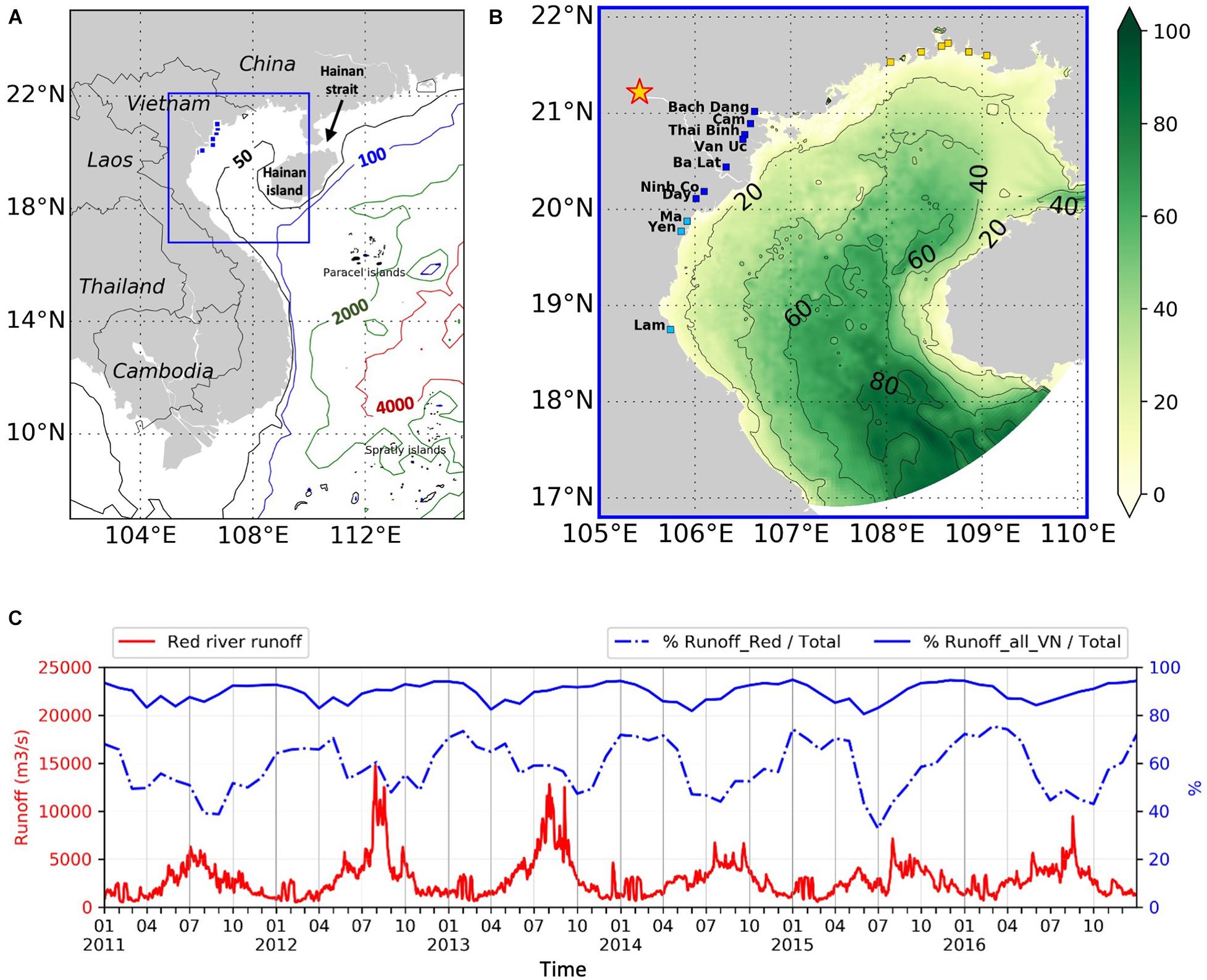
Figure 1. (A) Location of the Gulf of Tonkin. Blue dots show the location of the river mouths of the Red River system. Contour lines indicate the bathymetry of the area. (B) Model domain with bathymetry. The star indicates the location of Son Tay hydrological station at the apex of the delta. Blue boxes show the most upstream points where the runoffs flow to the model. Cyan and yellow boxes show the location of other river mouths in the south and north of RR, respectively. (C) Daily Red River discharge in the model configuration, from National Hydro-Meteorological Service data (red curve, left y-axis). Blue dashed line: Percentage of Red River runoff compared to total runoff (sum of runoff from Red River, other rivers in Vietnam, rivers in China). Blue line: percentage of all rivers in Vietnam (including Red and other rivers in the GOT) compared to total runoff. Blue lines are referred to the right y-axis.

One of the expected drivers of the dynamics is the freshwater input from the continent. In the GOT, several rivers feed the gulf. The main one is the Red River (hereafter RR) system. It is formed by 3 tributaries that connect at Son Tay (Figure 1B) and then split again into several distributaries. On average, the RR’s runoff accounts for more than 60% of the total runoff in GOT (Figure 1C).

In spite of its importance, to date, studies focusing on the RR plume are still scarce. Gao et al. (2013) showed that the coastal plume was found near the northern and western coasts of the gulf in winter while spreading eastward and offshore in summer. Rogowski et al. (2019) analyzed the mean seasonal circulation and suggested that the southwesterly wind direction which is prominent during the summer monsoon is the main mechanism preventing downcoast advection of the RR plume. However, that study did not attempt to explain further the temporal variations of the RR plume. In this study, we propose to take the analysis a step further and examine the plume variability in the mid-field and far-field regions (as defined by Horner-Devine et al., 2015) in more detail, using high-resolution simulations and an unsupervised learning method.

The objectives of this study are (1) to propose a method to identify the RR plume in the GOT from the model outputs, (2) to describe its development and characterize its variability at different scales and (3) to attempt to describe the physical processes at work. To do this, we use numerical simulations combined with cluster analysis. In section “Methods, Model, and Data,” the model configurations, data sources and the unsupervised learning algorithm used to classify the main pattern of the plume (K-means) are described. The model is then evaluated against several observational data sets in section “General Circulation and Model Assessment.” In section “River Plume in GOT: Identification and Variations of Area,” several methods to identify the plume in the GOT are compared which allows us to select the most appropriate one given our purposes. On that basis, the river plume variability at different time scales is examined in section “Variability of the RR Plume,” illustrating the effect of key physical processes. A discussion on the plume classification and a description of the receiving basins from the different river systems in the GOT are presented in section “Discussion,” followed by conclusions in section “Conclusion.”

Methods, Model, and Data

SYMPHONIE Model and General Configuration

SYMPHONIE is a numerical model that solves the primitive, Boussinesq, hydrostatic equations of the ocean circulation (Marsaleix et al., 2006, 2008) on a curvilinear bipolar (Bentsen et al., 1999). Arakawa C-grid with regular sigma vertical levels. The QUICKEST scheme is used for advection and diffusion of tracers (Neumann et al., 2011), while horizontal advection and diffusion of momentum are respectively computed with a 4th order centered and a bi-harmonic scheme, and vertical advection of momentum by a 2nd order centered scheme (Damien et al., 2017). The k-epsilon turbulence closure scheme is implemented as in Michaud et al. (2012).

Our reference configuration, hereafter called GOT_REF, is an update of the configuration of Piton et al. (2021). The model domain covers the GOT area. Due to the variable horizontal grid, the coastal area near the RR mouths has a fine horizontal resolution of 300 m, while near the open boundary, the grid size can increase to 4500 m (Figure 2A). As the coastal area adjacent to the RR delta is characterized by a complex topography, with many islands and islets, a considerable effort has been devoted to the construction of the model bathymetry and shorelines and is described in Piton et al. (2020). In particular, the bathymetry is reconstructed from GEBCO 2014 combined with other sources and field surveys. The bottom drag coefficient follows a logarithmic law (Blumberg and Mellor, 1987), depending upon the bottom roughness length which is set to 1 mm. The parametrization for the solar penetration depth (as described for instance by Maraldi et al., 2013) distinguishes the red and near-infrared radiations which are absorbed in surface layers (e-folding length scale: l = 0.35 m), and shorter wavelengths (mostly visible and ultraviolet) which penetrate deeper (e-folding length scale from less than 4 m along the coastline up to 15 m in the deeper region of the GOT).

FIGURE 2

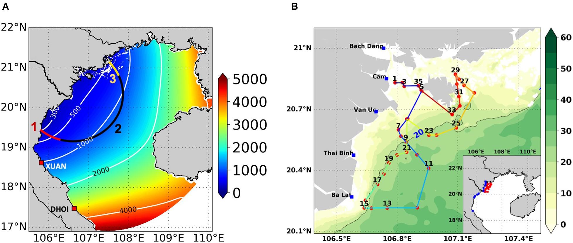
Figure 2. (A) Grid cell size (m). Red squares show the location of HFR antennas. (1, 2, 3): Sections used to calculate the tracer transport. VITEL (B) CTD stations location. Red dots indicate the station locations, while blue points indicate the river mouths’ locations.

Lateral boundary conditions, as described in Toublanc et al. (2018), allow the model to be nested into a larger scale model. At the open boundary, tidal surface elevation and current at K1, O1, P1, Q1, K2, M2, N2, S2, M4 frequencies from the tidal atlas FES2014 (Lyard et al., 2021) are taken into account as in Pairaud et al. (2008). The model is also forced by daily averages of sea surface height (SSH), 3D zonal velocity (u), meridional velocity (v), temperature (T) and salinity (S) fields, from the global analysis (hereafter ‘OGCM’) produced by Mercator-Océan International and provided by Copernicus Marine Service (CMEMS) at a resolution of 1/12°. CMEMS T, S fields are adjusted to recover consistency with tidal physics before being used at the open-boundary conditions of the model (APPENDIX A).

At the surface, boundary conditions are provided by an atmospheric model and fluxes of momentum, heat and freshwater are computed using the bulk formulae of Large and Yeager (2004). Operational ECMWF analyses (with a spatial resolution of 1/8°) are used to provide 3-h wind, precipitation, solar energy, atmospheric temperature, dew-point temperature, surface pressure.

As the present study focuses on the fate of continental water into the coastal ocean, a specific effort has been deployed on the river runoffs implementation; section “River Configurations” is dedicated to its description.

The model is run from 2010 to 2016, starting from the ocean state condition as provided by the global OGCM on 01/01/2010. The time step is set at 2 min. Further analyses are calculated during 2011–2016 (i.e., following a 1-year spinup). The model outputs include daily averaged variables as well as instantaneous fields every 12 h. Unless otherwise specified, both components of the current are detided based on an online harmonic analysis. A summary of the general configuration is available in Table 1.

TABLE 1

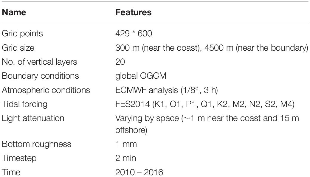
Table 1. General characteristics of GOT_REF.

Two other simulations are performed over the same period:

– a twin simulation without river forcing (GOT_NORIV) to assess the impact of the river runoff on the coastal circulation; all other forcings and parameters are the same as in GOT_REF.

– a twin simulation without tides (GOT_NOTIDE) to assess the impact of tides on the main patterns of the river plume variability; all other forcings and parameters are the same as in GOT_REF.

River Configurations

In most modeling studies to date, the RR was set up with only one mouth (or input grid point) using monthly or annual climatological runoff because more realistic runoff at the hydrological station was unavailable (Ding et al., 2013; Gao et al., 2013). In this study and in Piton et al. (2021), the river condition is configured as realistically as possible. Firstly, the delta is represented taking into account seven input grid points representing the mouths of the main RR delta distributaries (Bach Dang, Cam, Van Uc, Thai Binh, Ba Lat, Ninh Co., Day) (Figure 1B). Secondly, the daily RR runoff is obtained from the National Hydro-Meteorological Service (NHMS) of Vietnam at Son Tay hydrological station which is located at the apex of the RR delta. The discharge is distributed across the seven distributaries based on the results of Vinh et al. (2014) (Bach Dang (7%), Cam (13.2%), Van Uc (14.5%), Thai Binh (6.4%), Ba Lat (30.3%), Ninh Co (5.6%), Day (23.0%)). Furthermore, each river mouth is connected to a channel in the model to allow the water entering the coastal ocean with realistic salt and temperature properties and realistic stratification. The length of the channels (35–45 km, depending on the channel) is chosen to exceed the saltwater intrusion, which is approximately 30 km from the mouth (Nguyen Thi Hien et al., 2020). The results from GOT_REF confirm that the salty water never reaches the end of the channel, even in the low discharge period. The river runoff is converted into a vertically sheared current at the most upstream point of the channel (APPENDIX B); there the salinity of the river flow is 0 and the temperature varies seasonally from 17°C (in February) to 29°C (in August).

Other Vietnamese rivers (Ma, Yen, Lam) at the south of the Red River delta (hereafter referred to as the ‘southern rivers’) are also taken into account (Figure 1B). As daily runoffs were not available to us, we prescribe monthly climatological runoffs from NHMS. At the north of the Red River delta, 6 rivers (hereafter referred to as the ‘northern rivers’) are accounted for (Figure 1B), based on the data given by Gao et al. (2013). In general, the runoff of the Red River system alone accounts for 60% of the total runoff to the gulf, while adding other rivers runoff in Vietnam accounts for around 90% of the total runoff (Figure 1C). In detail, the average discharge for the Red River system in low (December, January, February) and high (July, August, September) discharge period equals to 1632 m³/s and 4959 m³/s, respectively. For the southern rivers, this value is 365 and 2043 m³/s. For the northern rivers, it is 164 m³/s and 1103 m³/s. It is clearly shown that for the Red River, the ratio between high and low discharge seasons is only 3 times, this ratio is 5.6 times for the southern rivers and 6.7 times for the northern rivers. The lower ratio of the Red River can be due to the presence of several hydrological dams upstream.

In order to simulate the pathways of the river water into the GOT, passive tracers are used. Tracers act as dyes, i.e., they do not affect the dynamics. In total, there are 3 tracers (or three colors) meant to distinguish the inputs from the different river systems. The first tracer is added to the runoff of all the Red River distributaries at constant concentration (100 arbitrary unit/m³). The second one is added at the other rivers in the south and the third one at the rivers in the north of Red River, with the same concentration (100 arbitrary unit/m³). Since tracers are injected with the runoff, they are also submitted to the 1 year of spin-up.

Observational Data Sets Used to Evaluate the Simulation

In situ Data

We use temperature (T) and salinity (S) profiles measured at 35 CTD stations (Figure 2B) during the VITEL cruise which took place in July 2014 (Ouillon, 2014). We further use CTD measurements of T, S acquired repeatedly at 10 stations along a 25 km cross-shelf section by Vietnamese and US teams from Center for Oceanography (CFO) and Oregon State University (Rogowski et al., 2019). This dataset, hereinafter referred to as CFO data, consists in 20 timeframes between September 2015 and July 2016.

We compare the simulated tidal amplitude and phase with historical tidal measurements from 13 stations (whose location is indicated in Figure 3). The dataset stems from the International Hydrographic Organization¹.

FIGURE 3

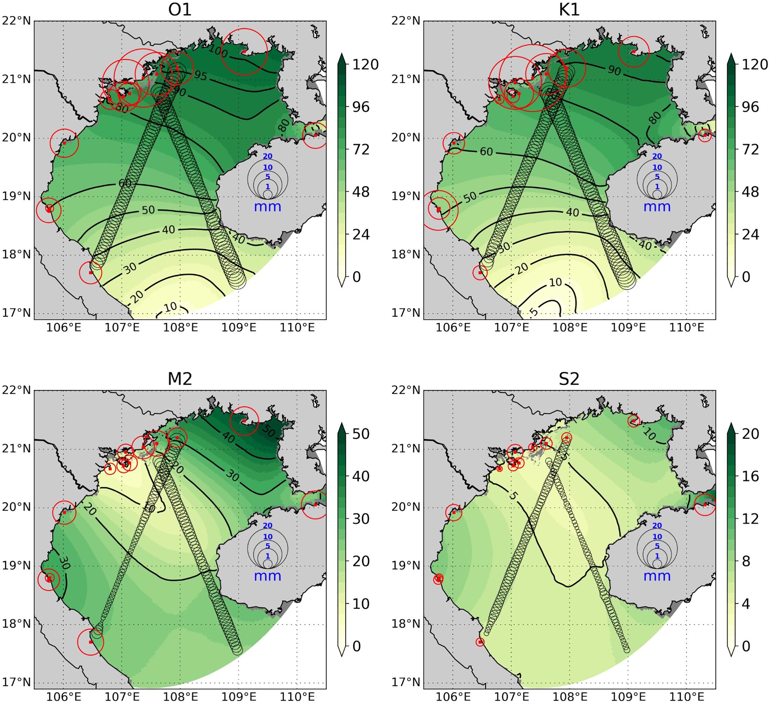
Figure 3. Amplitude of the tidal constituent (in colors, cm) from GOT_REF. Each figure shows the complex error (mm), calculated from the amplitude and phase, between model result and observational data for 4 main tidal constituents (O1, K1, M2, S2). Black circles show errors compared to altimetry data, while red circles indicate errors compared to the tidal gauges data.

High-Frequency Radar Measurements

We use surface velocity data from the high-frequency radar (hereafter HFR) system based on two antennas located at 18.62°N (XUAN site) and 17.47°N (DHOI site) (Figure 2A) along the coast and operated by the Center for Oceanography, Vietnam Administration of Sea and Islands (CFO, VASI). The data consists of daily maps of zonal and meridional components of the surface current, over the year 2015, built by Tran et al. (2021). The radial velocity measurements are gap-filled, interpolated onto a 6-km rectangular grid and detided as described by Tran et al. (2021). As explained in Rogowski et al. (2019), the summer coverage is lesser than in winter because of low sea state conditions; therefore uncertainties on the interpolated velocities are larger in summer. Comparisons with in situ measurement over a 12-day period indicate a mean bias of 3 cm/s and an RMS difference of 10 cm/s (Tran et al., 2021); we use these values as rough estimates of the data uncertainties. HFR data is representative of currents at 2.4 m below the surface (Tran et al., 2021); as a consequence, for the model assessment, we estimate the model current at 2.4 m before interpolating it over the HFR grid.

Altimetric Data

Tidal constituents computed from satellite altimetric data provide a rich dataset to evaluate the simulated tides offshore. Along-track amplitudes and phases are calculated from the long time series of sea surface height obtained from satellite altimetry (TOPEX/Poseidon, Jason 1–2) by using harmonic analysis. We use the dataset described in Lyard et al. (2021).

K-Means Unsupervised Learning Algorithm for Time Series Pattern Analysis

Many different methods exist to analyze the main characteristics of time series, such as statistical, spectral and classification methods. In terms of classification, there are several methods. For example, Self-Organizing Maps method is used to describe the river plume patterns by Vaz et al. (2018) for the Tagus River and Falcieri et al. (2014) for the Po River. Here, we apply another method, K-means, to analyze not only the plume patterns but the associated forcing conditions.

K-means clustering analysis (KMA) is a popular unsupervised learning method (Hastie et al., 2001) that allows to classify objects (observations, model outputs) into different groups, given a measure of dissimilarity.

The aim of this method is to iteratively identify clusters by their centroid (the means) then minimize the distance between each member of the cluster and the centroid of that cluster. The procedure of this method is made of six steps.

Step 1: Choose the number of clusters to compute.

Step 2: Allocate random numbers as the centroids of the clusters.

Step 3: Calculate the distance from each member to the centroids, using the Euclidian distance (see APPENDIX C for more details).

Step 4: compare these distances, then assign the member to the cluster corresponding to the minimum distance.

Step 5: for each cluster, re-calculate the centroid based on the mean of all members which belong to that cluster.

Step 6: repeat step 3 to 5 until the clusters no longer change.

This method has been used in several past studies in coastal oceanography. Solabarrieta et al. (2015) used it to examine the relationship between wind and surface circulation in the Bay of Biscay. They found that most of the current patterns are related to a specific wind pattern in the study area. Chen et al. (2017) identified the area of Pearl river plume by applying the K-means clustering to a summer climatological turbidity image. Sonnewald et al. (2019) used it to classify different regions based on the barotropic vorticity.

In this study, we use KMA to identify the main patterns of the plume and their temporal variations using daily model outputs. To do this, we use the KMA as implemented in the scikit-learn library coded in python (Pedregosa et al., 2011).

In the KMA method, the number of clusters is not fixed automatically, it is chosen depending on the application. The number of clusters should lead to an easy interpretation of the classification, since the objective is to reduce the dimension of the ensemble of scenes to analyze, without eliminating too much variability. In this study, we choose 4 clusters. The method to identify the number of clusters is described in APPENDIX C.

We applied KMA to the “masked river plume.” Firstly, plumes are identified using tracers (as described in section “River Plume in GOT: Identification and Variations of Area”). Then, for a given day (a scene), each grid point where the plume is considered to be present is masked with 1, while other points are masked with 0. The results of the classification are shown and analyzed in section “Variability of the RR Plume.”

General Circulation and Model Assessment

The main objectives of this section are to provide a general description of the patterns of the seasonal circulation at the scale of the GOT from GOT_REF, to assess the consistency of model results with previous studies (or evidence their specificities) and to provide a qualitative assessment by comparing to observations. As a description of the general circulation and model verification (in particular using satellite data) have been provided recently by Piton et al. (2021) from a very similar configuration, we do not provide a detailed analysis. We introduce the section by a discussion of the first Rossby radius, continue with the basin-scale circulation, evaluation of tidal elevation and with the comparison to in situ temperature and salinity data and surface current velocity from high-frequency radars in the area of the RR plume.

First Baroclinic Rossby Radius of Deformation

The first baroclinic Rossby radius of deformation (Rd) sets the scale of mesoscale baroclinic instabilities and, as such, should be resolved by the numerical circulation models (see for instance Greenberg et al., 2007). In river plume dynamics, Rd in the near-field or far-field (coastal current) is used to estimate the relative impact of Coriolis force on the plume dynamics with respect to other forcing (runoff, ambient current). For instance, Yankovsky and Chapman (1997) showed that for surface-advected plumes, the offshore extension is more than four Rossby radii.

In this study, Rd is computed from the mean seasonal field of temperature and salinity from our simulation over 2011–2016. The calculation is made by solving a Sturm-Liouville problem as described for instance in Chelton et al. (1998). We use the method developed by F. Lyard at LEGOS for free surface vertical modes of the internal pressure and described for instance in Nugroho (2017). At depths larger than 60 m, the Rossby radius decreases from 10 to 13 km in April–September (Figure 4A) to 4–7 km in October–March (Figure 4B). In shallower areas, it decreases from 3–8 to 1–5 km. Such a seasonal variation is expected as the stratification is stronger in April–September with higher air temperature. A large spatial variability is also observed; by construction it is correlated to the bathymetric variations. In particular, a striking feature is the eastward extension of the shelf, between the Bach Long Vi island and the coast; the Rd does not exceed 4 km there. Close to the coast in both summer and winter monsoon periods, it can drop to less than 1 km. Moreover, the Rd spatial variability also reflects some patterns of the circulation. For instance, a strong mixing occurs west of Hainan, mostly due to tides, as suggested in the literature (e.g., Nguyen et al., 2014; Piton et al., 2020) and in agreement with the local maximum of the K1 and O1 current in our simulation (Supplementary Figure 1). As a consequence, the Rd is only a few hundred meters west of Hainan Island. On the other hand, the RR runoff leads to an increase of stratification along the Vietnamese coast south of 21°N which has a clear signature in a locally larger Rd (∼4–5 km) in the October–March period.

FIGURE 4

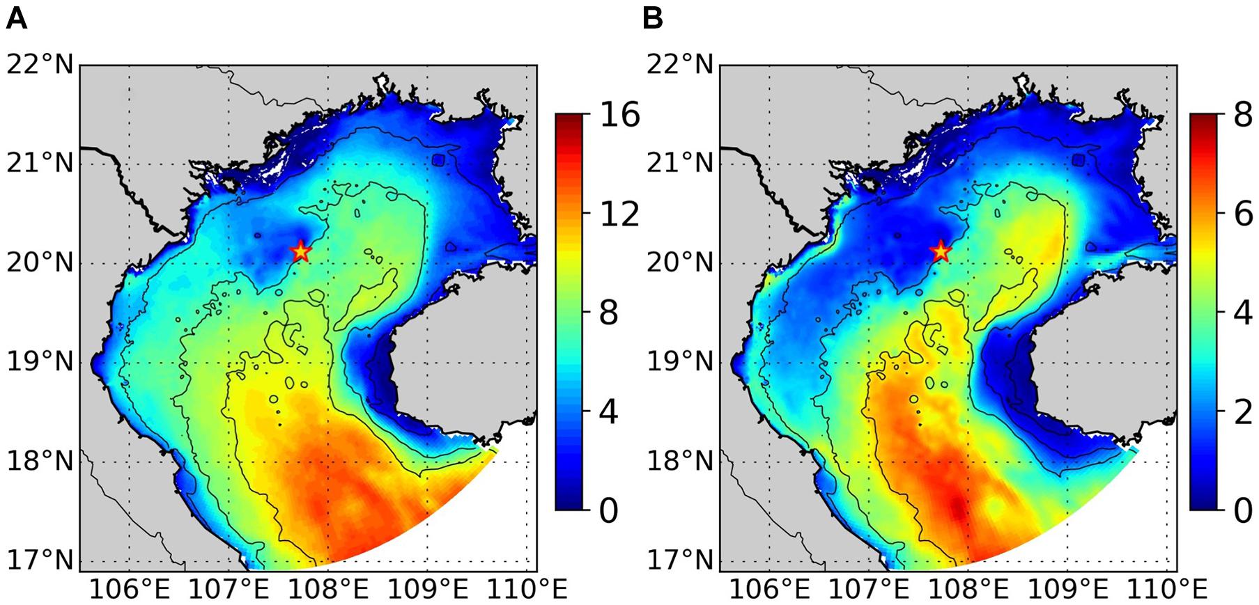
Figure 4. (A,B) The first baroclinic Rossby radius of deformation (km), over the period 2011 – 2016, computed from the temperature and salinity profiles averaged from April to September (A) and October to March (B). Contour lines indicate the bathymetry. Star shows the location of Bach Long Vi island. Note: Different color bar scales.

Assuming that the effective resolution is roughly between six and ten times its grid resolution, we can evaluate the model’s ability to resolve Rd. Rd is well resolved in the northwest quarter of our domain where the mesh is well refined in summer, and along the Vietnamese coast between 19 and 21°N in winter. However, if we consider that the scales of interest are about 4 times the Rossby radius, then the model resolution is sufficient between 18 and 21°N.

General Circulation

Mean Surface Circulation

The current in the GOT has been studied with mainly a focus on the northern region, due to the lack of observational data in the south (Wu et al., 2008; Ding et al., 2013; Gao et al., 2014). Recently, thanks to the deployment of a high-frequency radar system, the surface circulation in the southwestern area has been documented (Rogowski et al., 2019; Tran et al., 2021). However, the variability of the general surface and subsurface circulation remains relatively undocumented over the whole gulf and more specifically along the Vietnamese coasts.

Figure 5A shows the mean surface current from November to March from GOT_REF for the 2011–2016 period. The circulation in this winter monsoon period is dominated by the gulf-scale cyclonic gyre, as reported by several authors (Ding et al., 2013; Gao et al., 2014; Rogowski et al., 2019; Piton et al., 2021). The coastal current along Vietnam originates from the merging at 20°N of the westward flow from Hainan Strait and a coastal current from the northernmost shelf. It flows downcoast down to the southern boundary of the domain. It is the dominant feature of the surface circulation with a mean amplitude of about 30 cm/s. South of Hainan Island, an inflow from the South China Sea is simulated in the deepest part of the area with a decreasing intensity from November to March. This inflow is deflected westward and joins the coastal current south of 19°N, creating a small-scale cyclonic gyre as in Ding et al. (2013).

FIGURE 5

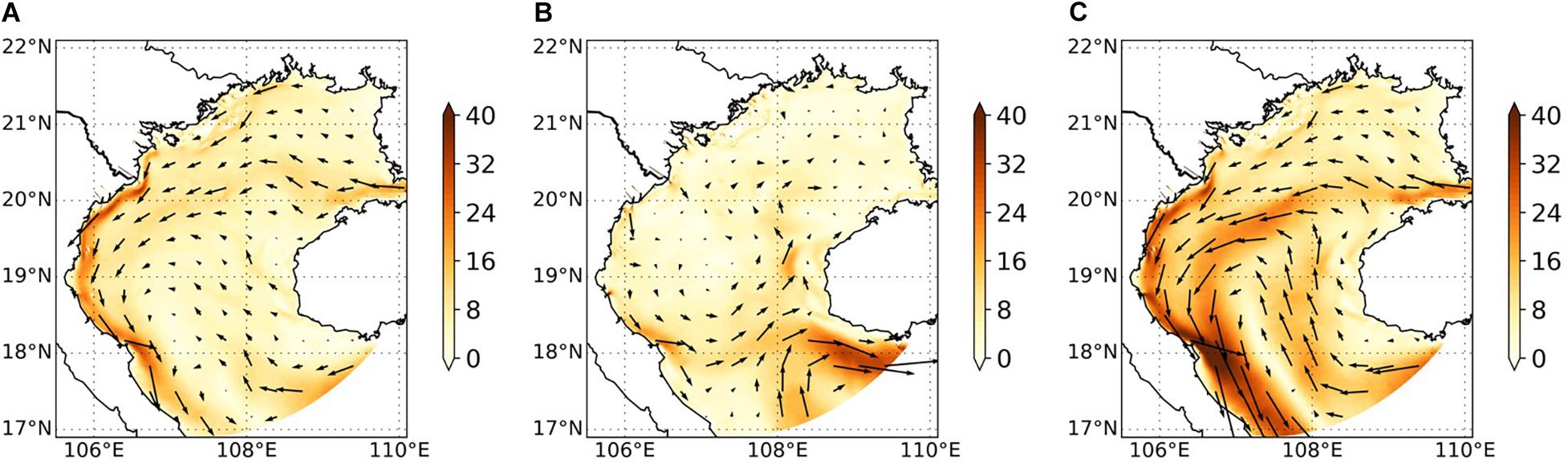
Figure 5. Means of the detided daily surface current (cm/s) simulated by GOT_REF. (A) November – March average. (B) April – August average. (C) September – October average.

In April, the summer monsoon sets in and lasts until August. The southward coastal current weakens and becomes intermittent (Figure 5B). When present, it is deflected eastward at ∼18°N; it then splits into 2 branches. The first one forms a cyclonic circulation in the central basin. The second branch feeds an intense current south of Hainan that flows out from the gulf. This corresponds to the circulation scheme described by Gao et al. (2014) and Rogowski et al. (2019), but, in our simulation, the current variability is large at daily and interannual time scales.

In September and October (Figure 5C), the coastal current is southward again from 21°N to the southern boundary where it exits the gulf. It reaches its maximum amplitude (∼35 cm/s) and width. Besides, the circulation is characterized by two inflows with large velocity (∼30 cm/s): one from Hainan Strait and the other from the southern boundary in the deep region.

Horizontal Transport

The horizontal transport displays a similar seasonal cycle as the surface current. From September to March, the general circulation is cyclonic, with a large downcoast transport over the shelf in the west. From April to August, the transport inside the gulf weakens significantly. The main specific patterns are a cyclonic gyre in the central area.

The flow direction during the summer monsoon through Hainan Strait is discussed in several papers (Shi et al., 2002; Gao et al., 2013; Chen et al., 2017). In our simulation, the flux is inflow from September to April and an outflow during the summer monsoon. It varies between −0.18 Sv and +0.15 Sv at 110 E, with significant daily and interannual variability (not shown). Our results however are consistent with the situation described by Wu et al. (2008); in case of inflow the circulation is mainly cyclonic, while in case of outflow the overall circulation is anticyclonic.

Besides, the gulf is fed all year long by an inflow from the southern boundary, which is maximum in summer monsoon period. From September to December, it enters through the east and either penetrates northward in the gulf or is deflected westward and joins the coastal current. The rest of the year it enters through the center, is deflected eastward and generates a large outflow south of Hainan Island.

Model Assessment

Evaluation of Tides

The simulated amplitudes in terms of sea surface elevation for the four main tidal constituents (O1, K1, M2, S2) are shown in Figure 3. O1 and K1 have the same amplitude distribution. The amplitude is largest in the north (100 cm and 95 cm for O1 and K1, respectively) and decreases to its lowest value at the south of the gulf, near the boundary. M2 has two peaks of amplitude. One peak is located in the north (50 cm) and another peak is located at 19°N (30 cm) along the Vietnamese coast. The lowest amplitude is located near RR mouths. These patterns are similar to the ones found by Nguyen et al. (2014) and Piton et al. (2020). We also examined the tidal currents (see Supplementary Figure 1): the O1 and K1 tidal currents are the strongest west and south of Hainan Island and in the Hainan Strait (more than 50 cm/s). Near the Vietnamese coast, they are weaker and range from 10 to 20 cm/s. They reach a local maximum (∼ 30 cm/s) along the coast at ∼18°N, 106.5°E. M2 tidal currents vary between 10 and 20 cm/s, with a local maximum close to the Ba Lat mouth. S2 currents have a similar spatial distribution but smaller amplitude (<4 cm/s close to the RR mouths).

The simulated tides show remarkable comparisons to along-track altimetric data (Figure 3): the root mean squares of the complex errors (i.e., the model-data misfits) over the domain are as low as 2.6 cm, 2.8 cm, 1.3 cm, 0.7 cm for O1, K1, M2 and S2, respectively. These values correspond to 5.0%, 6.0%, 7.4%, and 12.9% of the signal. The model-data misfits are homogeneous in the center of the basin. They are the largest near the coast as expected due to the larger uncertainty of both the altimetry data near the coast and due to the uncertainty of model bathymetry in the very shallow area. These values are comparable to those obtained by Piton et al. (2020) with the T-UGOm tidal model over the same domain (2.6 cm, 3.5 cm, 3.0 cm, and 1.2 cm for O1, K1, M2 and S2, respectively) and to those of Nguyen et al. (2014).

Compared to historical tidal gauges data, the complex error is larger: 18.3, 20.9, 6.2, and 2.3 cm for O1, K1, M2, S2, respectively (Figure 3). There are several reasons for these higher errors. Firstly, the observation period for the tidal gauges data that are available is relatively short (15 days to 1 year) and may not be long enough to be accurate and representative of ‘mean’ tides. Secondly, the largest errors are observed in the area of the RR delta where the extremely complicated coastline with the presence of thousands of small islands makes the accurate representation of tides a challenge for such a configuration. Compared to Piton et al. (2020), GOT_REF performs better for M2 (6.8 cm) and S2 (3.5 cm), but gives poorer results for K1 (10.2 cm) and O1 (10.2 cm). Future work will be dedicated to tuning the properties of the channels (see section “River Configurations”) to better simulate the propagation of the tidal wave in the delta.

Comparisons With High-Frequency Radar Currents

Figure 6 shows the data from the HFRs and from GOT_REF in different seasons in 2015, as well as the maps of correlation between simulated and observed u and v over the whole time series (1 year).

FIGURE 6

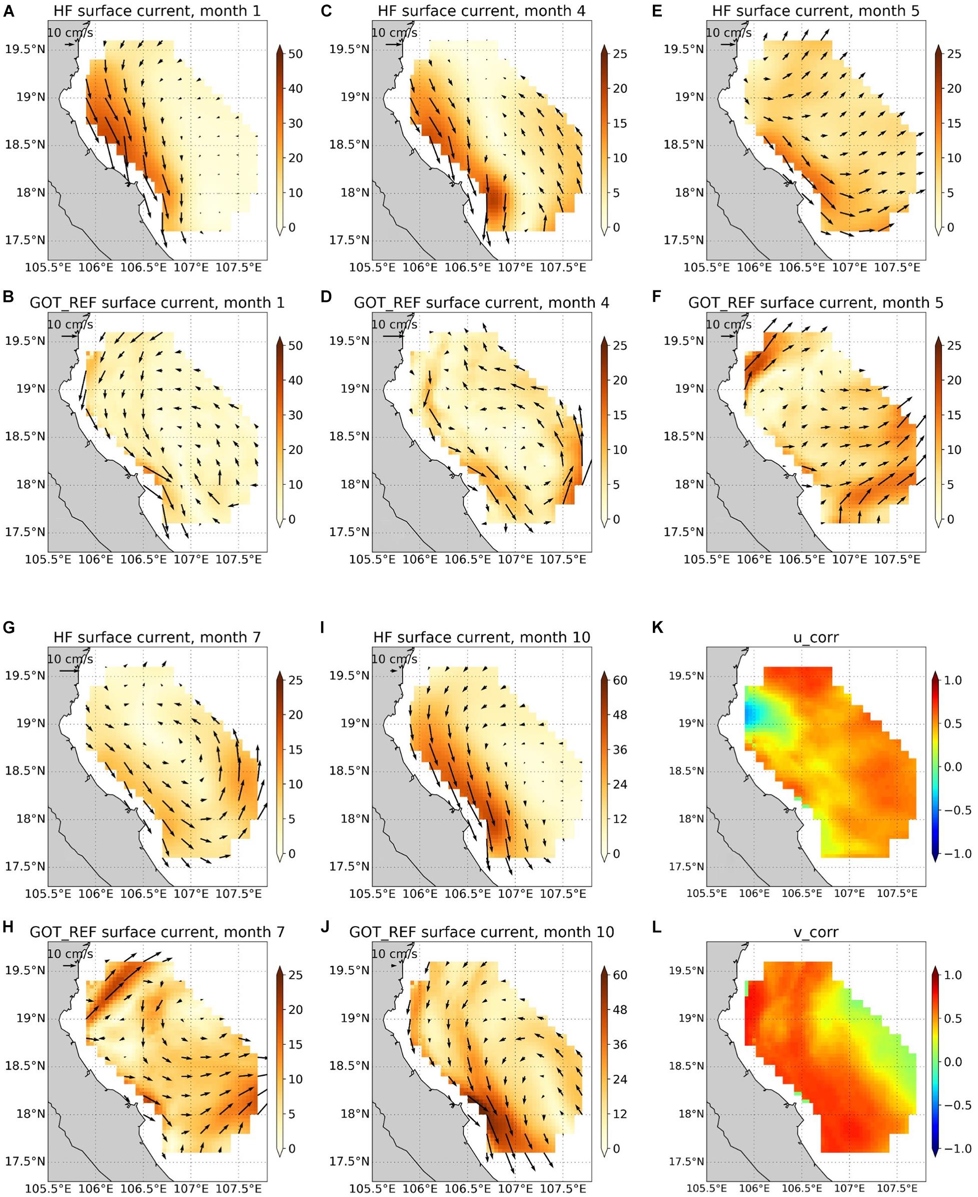
Figure 6. Surface current from HFR data (A,C,E,G,I) and model simulations (B,D,F,H,J) for different months of 2015 (Jan, Apr, May, Jul, Oct) (cm/s). Temporal correlation of u and v (K,L) computed from daily currents. Note: Different color bar scales.

In January, the main observed coastal current is southward, with an amplitude of ∼ 30 cm/s at the coast and decreasing offshore. The model shows the same current direction, but its amplitude is underestimated by 20 cm/s (Figures 6A,B). In April, the coastal current is less intense, but the northward current at 107–107.5°E is stronger. In GOT_REF, both the southward and northward circulations are observed, with a persistent underestimation of the coastal current regarding the HFR data (Figures 6C,D). In May, the coastal current reverses north of 19°N in both the observations and simulation. At around 18°N, the simulated downcoast current is deflected eastward consistently with the HFR observations. However, both at 19°N and 18°N the simulated current is stronger than in the HFR data (Figures 6E,F). In July, HFR data show a nearly closed circulation. The coastal current flows southward at 19°N, then rotates at 18°N and flows northward and finally joins the coastal current at 19°N again. In GOT_REF, the circulation shows a more complex pattern, with a northward current (of ∼20 cm/s) at 19°N and a large temporal variability (Figures 6G,H). In October, HFR data show a similar current pattern as in January, with a strong southward coastal current (∼40 cm/s). The model shows very good consistency, with the strongest velocity near 18°N (Figures 6I,J).

The temporal correlation between simulated and observed daily fields of u and v is higher for u offshore (∼0.5) (Figure 6K), while the correlation for v is better near the coast (>0.6) (Figure 6L). The larger misfits between the model and data at ∼19°N seem to come from a larger spatial variability of the simulated u component (not shown) than the observed one. In particular, as discussed in section “Variability of the RR Plume,” this area is characterized by some eddy activity in summer which may not be resolved by the HFR observations or may be out of phase with the observations.

Temperature and Salinity Profiles From in situ Measurements

Figure 7 shows the salinity and temperature profiles from the VITEL campaign and the GOT_REF simulation. Although it is a very shallow area, the bathymetry of the model is quite accurate compared to the depth of the CTD data. The largest bathymetry misfit is reached at stations 26 to 30 where the model is too shallow by ∼10 m. Since the campaign took place in summer (July), there is a strong stratification in both salinity and temperature profiles. At the surface, the observed salinity can be as low as 15, while at the bottom it is around 34. The mean value at all points is 28.7. The model performance is good, with a correlation R = 0.88 computed from all profiles, but the mean value is overestimated by 0.7. The model overestimates the surface salinity at stations located in the shallowest area. This suggests that the river runoff is underestimated or that the simulated mixing in the estuaries is too strong, possibly due to local errors on the tidal representation.

FIGURE 7

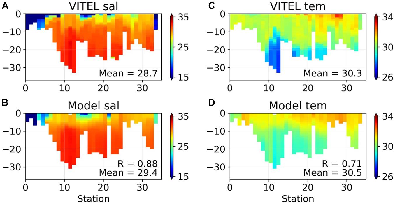
Figure 7. Profiles of salinity from VITEL data (A) from GOT_REF (B). (C,D) Same but for temperature.

The observed temperature goes up to 33°C at the surface and 27°C at the bottom, with a mean value of 30.3°C. The mean bias of the model is low (0.2°C), although the temperature is overestimated at both the surface and bottom at some stations. Overall, R is 0.72.

The comparison with the T, S profiles from the CFO campaigns is not described in detail as we get similar results to those described by Piton et al. (2021) in a similar configuration of the model. For all the 20 sections available, the mean biases (absolute value) between data and model are 0.61 and 0.71°C for S and T respectively, and the mean correlations 0.81 and 0.72. The comparisons suggest that the model runoff is not high enough (as already suggested by the comparison with the VITEL data), or the background salinity provided by the boundary condition is too high. The vertical mixing seems underestimated also. Overall, despite small biases, the model reproduces accurately the seasonal conditions even in the very shallow area.

River Plume in GOT: Identification and Variations of Area

This section will first review some past studies on plume identification then explains our method to identify the plume locally in the GOT. Then, the resulting variations of the plume area in the period 2011–2016 are analyzed.

A Brief and Non-exhaustive Review of Past Studies

There are no clear criteria to identify a river plume in general. Usually, such criteria involve sea surface salinity (hereafter SSS) because the river plume has a lower surface salinity than the surrounding ambient waters. However, due to different environmental conditions, the reference salinity is difficult to set in a general enough manner. In some studies, the authors may choose a suitable value based on their knowledge and experience; however, the choice is seldom justified in a rigorous way. This may lead to a situation where different authors choose different values for the same plume, depending on the observational or modeling approach and the objectives. For example, for the Columbia river plume, Liu et al. (2009) use SSS = 29 to detect the plume, while Burla et al. (2010) use the value of SSS = 28 and in MacCready et al. (2009) the plume is identified using SSS < 31.

Other authors defined other criteria to identify the plume. Otero et al. (2008) use the highest horizontal gradient of mixed layer depth to classify the river plume area in the Northwest Iberia and then use the SSS value of 35.6 that coincides with this maximum gradient. Another approach to identify river plumes is based on ocean color satellite images that reveal turbid water masses rich in Chlorophyll, suspended matter, or colored dissolved organic matter (e.g., Chen et al. (2017) for the Pearl River).

To our knowledge, there have been very few studies dedicated to the RR plume, so there is no published reference ambient salinity value. Rogowski et al. (2019) locate the RR plume using monthly means of ocean color maps from MODIS. In tropical areas, the presence of clouds is however a limitation to the use of optical products to investigate the sea surface variability at time scales shorter than a month.

Stratification Index and SSS Threshold

To identify the RR plume, different methods are in consideration in this paper. Firstly, we apply a method based on the Stratification Index (hereafter SI), assuming that the river water forms a buoyant layer over the ocean water. This index was first proposed by Hansen and Rattray (1966) for estuary classification. It is defined as the relative difference between the surface and bottom salinity (eq. 1). In this paper, we tested this method with a threshold of 0.1. If SI equals or exceeds 0.1, the water column is defined as belonging to the river plume. The time series of the daily plume area for all the rivers in GOT based on SI is shown in Figure 8A. As expected, the river plume area varies with the river runoff. In July–August (high runoff period), the plume area reaches its highest value, while it is lowest in December–January (low runoff period).

$$SI=\frac{salinit{y}_{bottom}-salinit{y}_{surface}}{verticalmeansalinity}(1)$$

FIGURE 8

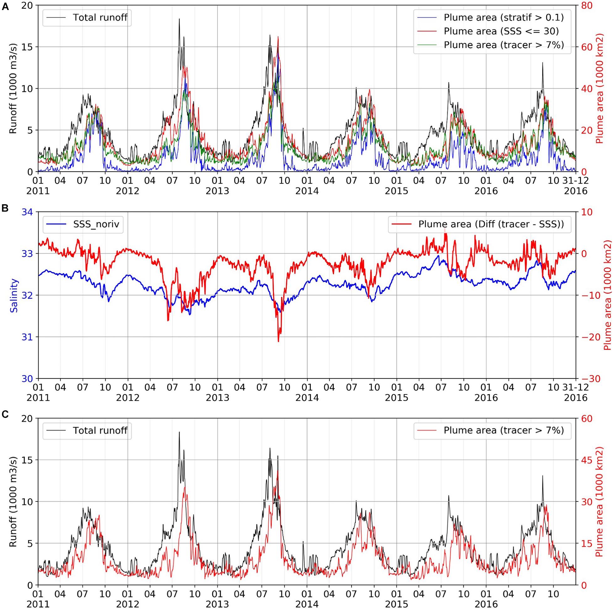
Figure 8. (A) Total runoff (in m³/s) and plume area (in km²) for all the rivers in the Gulf of Tonkin. The plume area is calculated using the Stratification Index (blue), SSS (red) and tracer concentration (green). (B) Spatially averaged SSS over the whole domain (in blue) from the simulation without river (GOT_NORIV), and difference of river plume area between SSS and tracer methods (in red). (C) Daily runoff and plume area for the Red River and Southern rivers.

However, there is one major drawback to the SI method. Vertical salinity sections indicate that the plume in the GOT consists of 2 zones. One is the very shallow coastal area where the plume is mixed over the entire water column; in the second one, farther offshore, the plume is detached from the bottom and stays on top of the high salinity water. SI being based on the difference between the salinity at the top and the bottom of the water column, it cannot detect the plume zone in the shallow area where it is totally mixed. In the low runoff period, as we will show in section “Variability of the RR Plume,” the downcoast current and the northeasterly wind make the plume stick to the coast; in such a case, the whole plume is well-mixed and SI is not helpful since the calculated area is close to zero (Figure 8A).

To deal with that problem, in a second step, we considered using SI as a proxy to find the suitable SSS that can be used as the plume indicator. After several experiments, we selected the value of SSS = 30. In high runoff period, this criterion defines a plume with a similar pattern offshore to the one deduced from the SI criterion. In the low runoff period, this discriminant value also captures the narrow plume area that runs along the coast (Figure 8A).

Using SSS, the envelope of river plumes created by all the rivers in the GOT was generally identified. However, this “stratification-based SSS” method has in turn two drawbacks. Firstly, it cannot distinguish the plumes created by the different rivers that feed the GOT. Secondly, the SSS criterion may be slightly biased at seasonal time scales by the effect of precipitation. Indeed, the precipitation has seasonal variations due to the monsoon system. The average precipitation from January to March is 1.8 mm/day, while it is 5 times higher (9.4 mm/day) from August to October (calculated from ECMWF daily precipitation over 2011–2016).

Passive Tracers

As an alternative method, we use passive tracers that behave in the model as any buoyancy-free particle or passive chemical from the rivers (as explained in section “River Configurations”). This is particularly relevant to identify the coastal area influenced by the river input of contaminants and to distinguish the freshwater input from other sources than the river such as advection by coastal current and other coastal runoffs [see for instance Wang et al. (2014) for the Copper River in the Gulf of Alaska] or to study mixing between the plume and ambient waters [e.g., Vlasenko et al. (2013) for the Columbia River]. As for the SSS criteria, the choice of a tracer concentration threshold to define the plume is author-dependent. In Vlasenko et al. (2013), the river plume is identified as the area where the concentration exceeds 10 units/m³ while in Wang et al. (2014), the threshold is 5 units/m³. In our study, several experiments led to identify the river plume as the area where the concentration exceeds 7 unit/m³, which best fits with the area identified by the criterion on SSS in the low runoff period (dry season).

As indicated in section “Observational Data Sets Used to Evaluate the Simulation,” 3 tracers were added, respectively to the RR distributaries, the southern rivers and the northern rivers. Figure 8A shows the plume area for all the rivers in the GOT calculated by summing the three tracers’ concentrations. The plume areas computed from the SSS and tracer criteria have a similar trend in both the low and high runoff periods. However, in the high runoff period, especially during the peaks in 2012 and 2013, the plume area calculated from the tracer is much lower than from the SSS. This difference can go up to over 20,000 km² (Figure 8B). Figure 8B also shows the SSS of the twin simulation without any river runoff (GOT_NORIV). Even with no river, the SSS shows significant variations between 31 and 33. The low sea surface salinity often happens in summer, which is in the rainy season. It is minimum in 2012 and 2013, which are also the years when the runoff reaches the highest peaks (Figure 8A), hinting at a correlation between local precipitation and runoff in both years. The SSS drop in the GOT_NORIV run has a similar trend than the difference of plume area calculated by the two methods, which suggests that this difference could be indeed due to precipitation.

In conclusion, for our objectives, the method based on the passive tracers seems the most appropriate to help identify the RR plume among the three methods investigated in this study. It can capture the plume in both the highly stratified zone and the shallow mixed zone. Besides, it can distinguish the plumes created by different rivers (as discussed in section “Discussion”).

Temporal Variability of the Plume Area

South of 20°N, the RR plume is quickly joined by the plumes of the southern rivers (Ma, Yen and Lam, Figure 1), creating a unique buoyant plume which extends southward along the coast most of the year. In this section and in the following we therefore analyze the variability of the resulting plume from the RR and the three southern rivers together. Section “Discussion” will discuss the receiving basins by distinguishing the RR from the other rivers, thanks to the multi-tracer approach.

Figure 8C shows the evolution of the cumulated runoff from the Red, Lam, Yen and Ma rivers and the corresponding plume area from 2011 to 2016. As expected, the plume area follows the same variations as the river runoff, albeit with a time lag. In summer, when the runoff is high, the peak of the plume area occasionally reaches more than 40,000 km² (about 27% of the GOT area), while in winter, it sometimes falls below 2,000 km². Due to the interannual variability of the runoff, the plume area varies significantly between different years. The river plume area peak in 2013 (41,000 km²) is nearly twice as large as the peak in 2015 (22,000 km²). Both the total discharge and the plume area undergo a strong variability at shorter time scales of a few days as well.

Figure 8C also shows two more characteristics of the plume variability. Firstly, a higher runoff does not ensure a larger river plume area. In 2012, the runoff peak is higher than in 2013, while the plume extension in 2013 is larger. Similarly, although the rainy seasons in 2014 and 2015 are characterized by similar runoffs, the plume area in 2015 is much lower than in 2014. Secondly, there is a time lag between the runoff peak and the peak of the plume area. This lag is also described in Rogowski et al. (2019). Depending on the year, it can be up to 1 month (in 2013). In 2015 and 2016, the plume area is relatively small until July and reaches its peak value rapidly within a few days. In short, both the time lag and plume area do not appear directly correlated to the runoff intensity (i.e., a higher runoff will not necessarily create a larger plume area about 1 month later). Such a variability evidences the fact that river runoff intensity is not the only factor driving the plume size and variability. Wind variability and its impact on the surface circulation and mixing is likely to be another driver, as we show in the next section.

Figure 8C displays as well some interannual variability in both the runoff and the plume area variations. The years 2015–2016 were marked by an intense El Nino event. Generally, El Nino events lead to decreased rainfall, drought and saltwater intrusion in deltas in Vietnam (Sutton et al., 2019). Figure 8C does not evidence a drastic drop in the 2015–2016 runoff with respect to 2014 and 2011. However, the SSS signal in the GOT_NORIV run is significantly different in 2015–2016 with respect to the previous years (Figure 8B): the mean SSS stays above 32 and the seasonal signal is inverted with a maximum SSS in summer. El Nino is likely to influence the coastal circulation, through alteration of wind and air-sea fluxes of freshwater and heat. The specific influence of ENSO on the coastal plume will be investigated in future studies as we focus in this paper on seasonal and shorter time scales.

Variability of the RR Plume

Spatial Patterns of the Plume

In the previous section, the river plume in GOT has been identified using passive tracers. We have documented the time variations of the total surface area and compared them to the runoff variations. Now, the seasonal variability of the plume spatial patterns is examined using KMA.

Figure 9 shows the spatial distribution of frequency of occurrence of the plume within each of the 4 clusters calculated from the plume area from 2011 to 2016, and the temporal evolution of the clusters, revealing both seasonal and interannual variations. The main variables of interest (SSS, wind, surface current, SSH) are averaged over the period corresponding to each cluster and are shown in Figure 10.

FIGURE 9

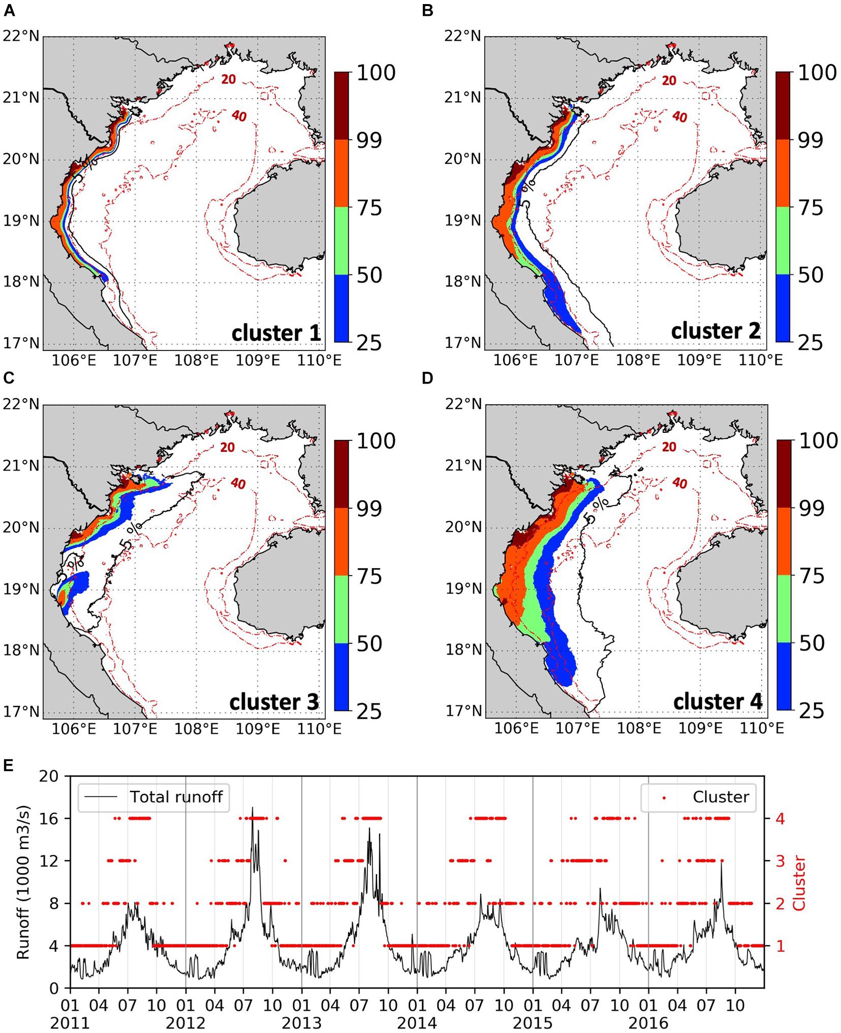
Figure 9. Frequency of occurrence of the plume within cluster 1 (A), cluster 2 (B), cluster 3 (C), cluster 4 (D). For instance, for cluster 1: at a given point, a frequency of 25 means that over the whole period when cluster 1 is present, the plume is present at this point 25% of the time. (E) Temporal distribution of each cluster (in red) and the runoff from Red and Southern rivers (in black).

FIGURE 10

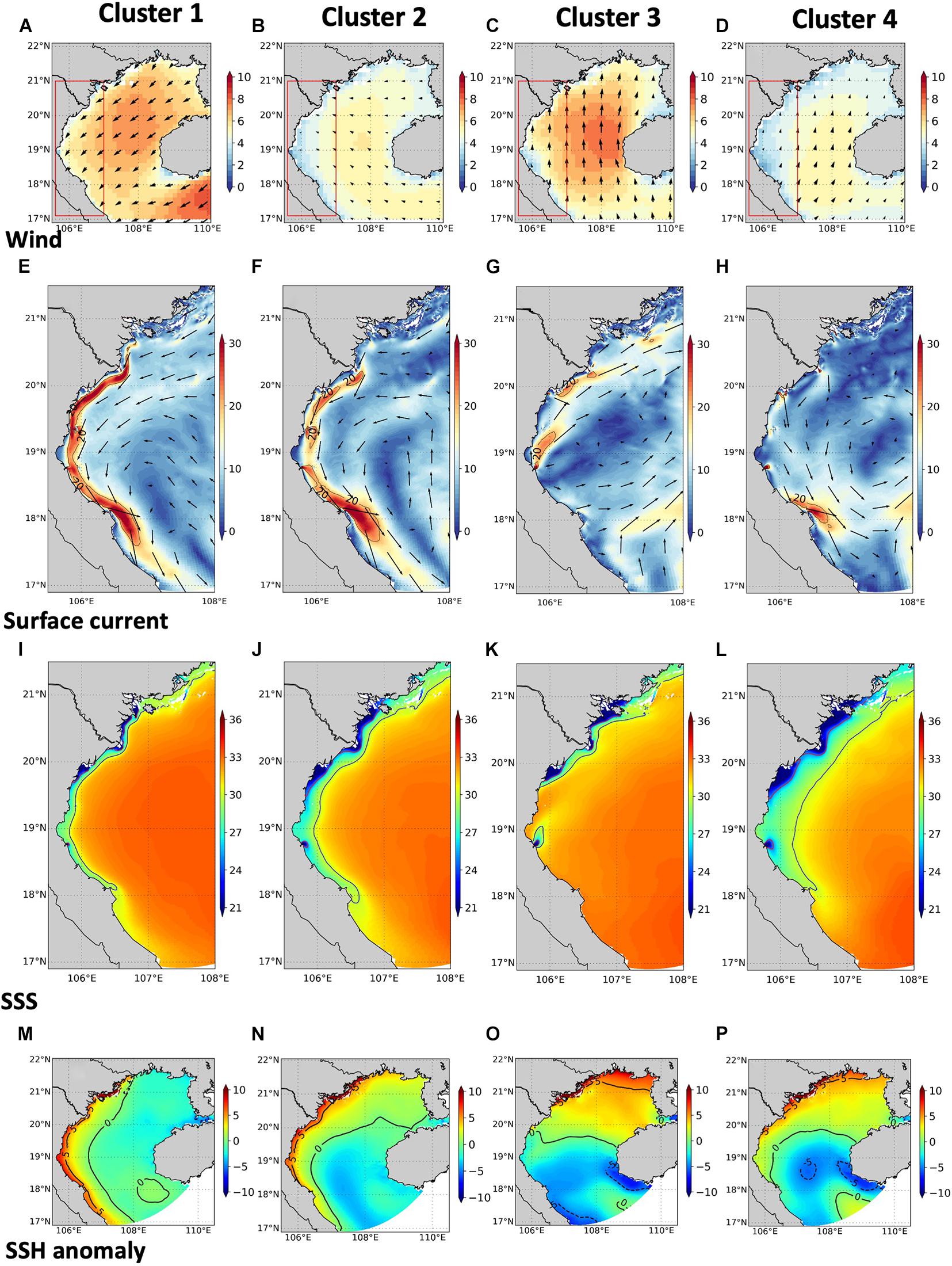
Figure 10. (A–D) Wind conditions (m/s) corresponding to the 4 clusters. (E–H) and (I–L) Same as (A–D) but for surface current (cm/s) and SSS. (M–P) SSH anomaly with respect to the mean over the basin for each cluster (cm).

The first cluster usually occurs from October to March and appears on 992 days (45.3%) in 6 years. In this cluster, the plume is very narrow and is mostly confined to the shallow area (depth < 20 m). 75% of the time that the plume occurs, at 19°N, it extends to 105.8E (∼20 km from the coast) while 25% of the plume extends to 105.85E (∼25 km from the coast) (Figure 9A). If the runoff (or other forcing) undergoes strong fluctuations, the plume area should also vary. In this cluster, the difference between the spatial occupancy of 25% and 75% is small: it means that the forcing condition is relatively stable. The simultaneous occurrence of several conditions can explain the relatively small extent of the plume in this cluster. Firstly, it happens in the lowest runoff period (average discharge over the cluster equal to 2197 m³/s). Secondly, the wind is strong and from the north-east (winter monsoon, Figure 10A), which is downwelling-favorable. At the GOT scale, the mean wind velocity is 6.4 m/s; it is stronger than in any other cluster, even near the coast (it reaches ∼ 5.7 m/s on average inside the red box shown on Figure 10A). The coastal surface current is southward, with a mean speed larger than 20 cm/s between 20.5 and 17.5°N (Figure 10E); consistently with the strong monsoon wind, the current also reaches its largest intensity in cluster 1. All these conditions favor the low salinity (SSS < 30) water to be confined to the coast and to extend southward all along the coast (Figure 10I). We also observe a cross-shore gradient of SSH with an elevation larger than 5 cm with respect to the basin-averaged SSH (Figure 10M). Here, the coastal current is fed by buoyant river waters which contribute to the geostrophic component of the current. Indeed, in the GOT_NORIV simulation, the surface current in cluster 1 is 10 to 15 cm/s weaker; the SSH is 1 to 4 cm lower (not shown). Similarly, Piton et al. (2021) estimate that the geostrophic contribution to the downcoast surface current reaches up to 60% in December-February.

The second cluster appears on and off throughout the year, with a slightly greater rate of occurrence in April and September (usually before the occurrence of cluster 3 and after the one of cluster 4), and accounts for 518 days (23.6%). It happens mostly in late spring and early winter, i.e., during the seasonal transition of the monsoon. This suggests that cluster 2 represents a transition regime for the river plume. In this cluster, the river plume extends both further offshore and further southward compared to cluster 1.75% of the time, the plume extends to 105.85°E (∼25 km from the coast) while 25% of the time, it extends to 106°E (∼40 km from the coast). The low salinity strip defined by the 30 isohaline is about twice as wide as in cluster 1 (Figure 10J). 50% of the time, the plume reaches 18°N, which is the same as in cluster 1, while 25% of the time, it extends as south as 17.1°N (Figure 9B). The higher spatial coverage of the plume area in this cluster can be explained by the higher runoff (4020 m³/s) than in cluster 1 (2197 m³/s). Also, in this cluster, the wind direction is from the southeast, therefore different with respect to cluster 1 (Figure 10B). The wind speed is weak, with a mean speed of 4.3 m/s near the coast (4.7 m/s at the gulf scale). The downwelling effect is relaxed and the light plume water can spread seaward. The coastal current is still flowing southward but is weaker than in cluster 1. As in cluster 1 and cluster 4 (see below), it is locally intensified, around 106.5°E, 18°N. The tidal current is intensified there as well (Supplementary Figure 1), probably because this is an area where the shelf is thinning and the coastline draws a cape. When present, the coastal current may be intensified there, through the same processes as for the tidal current. Another assumption is that interactions between tides and the coastal current occur there and result in an intensification of the local circulation.

The third cluster, which happens primarily in June and July (315 days, 14.4%), has a different shape with respect to clusters 1 and 2 (Figure 9C). In this cluster, the plume is advected northward and seaward. This is also the cluster in which the river plumes from the various rivers are disjoint. It corresponds to the period when the runoff increases with the mean value equal to 4631 m³/s and the summer monsoon wind reaches its strongest intensity. The mean gulf-scale wind speed is 5.7 m/s (5.6 m/s inside the box). It blows northeastward therefore corresponding to upwelling conditions. The surface coastal current is not present anymore south of ∼18.7°N; at 18°N the surface current is oriented seaward, with weak speed (∼10–15 cm/s). North of 18.7°N, the coastal current is reversed, flowing northward, with a weaker speed than in cluster 2 (∼15 cm/s), but locally intensified by the river runoffs. Although the average runoff is larger than for cluster 2, the very low salinity strip (SSS < 25) is smaller than in cluster 2, suggesting that strong mixing is taking place, either vertically due to wind-induced turbulent kinetic energy or horizontally. Figure 9C shows that 5% of the time, the plume reaches the 40 m isobath, and indeed the salinity over this area is decreased with respect to cluster 2, supporting the hypothesis of lateral mixing and/or stirring. The involved processes are assumed to be at daily timescales or shorter (inertial, tidal time scales) and are discussed in section “Variability of the Plume Dynamics at Daily Time Scales.”

The fourth cluster exhibits the largest spatial coverage and occurs mostly in August and September (367 days, 16.7%), that is at the peak of the high runoff season (the mean runoff over this cluster reaches 7336 m³/s). In this cluster, the plume extends the farthest offshore. At 19°N, it can extend to more than 100 km from the coast. 75% of the plume extends to ∼55 km from the coast, while 25% of the plume extends to 100 km from the coast. 5% of the plume can extend as far east as 107.0°N, which is 145 km from the coast (Figure 9D). In this cluster, the mean wind pattern is still upwelling-favorable, i.e., capable of driving the plume offshore (Figure 10D). However, the wind speed is less intense: 4.5 m/s at the gulf scale and 4.0 m/s inside the box only. It is the period with the lowest wind speed and the weakest coastal current; the latest is downcoast again. Its speed does not exceed 10 cm/s (except around 106.5°E, 18°N where it is locally accelerated up to more than 20 cm/s as in clusters 1 and 2, Figure 10H). The plume is surface-advected, which is verified by the analysis of the plume thickness in the next section. The large runoff during the August–September period is responsible for the very low salinity (SSS < 25) simulated along the coast between 21°N and 19.5°N. As for cluster 3, the salinity over the whole shelf in the western half of the GOT is decreased in this cluster, with respect to the previous one, indicating a larger extent of the river water influence than the one formalized by the plume definition that we adopted in section “River Plume in GOT: Identification and Variations of Area.” In other words, even highly diluted in the ocean waters, the river water is still influencing the ocean SSS. The comparison between the reference run and the run without runoff (GOT_NORIV) confirms that the runoff influences the SSS all over the gulf in clusters 2, 3 and 4 (Supplementary Figure 2), with the largest influence in cluster 4 (more than 1 west of 107°N and north of ∼20.5°N). The SSH shows a small elevation between the center of the basin and the Vietnamese coast, consistently with a weak downcoast circulation (Figure 11P). In GOT_NORIV, the SSH east of 107°E is decreased by 1 to 2.5 cm with respect to REF (not shown), while the surface current only differs from the REF run locally and the differences are smaller than for cluster 1 (and to a lesser extent for cluster 2), therefore suggesting a weak contribution of the riverine waters to the circulation in late summer.

FIGURE 11

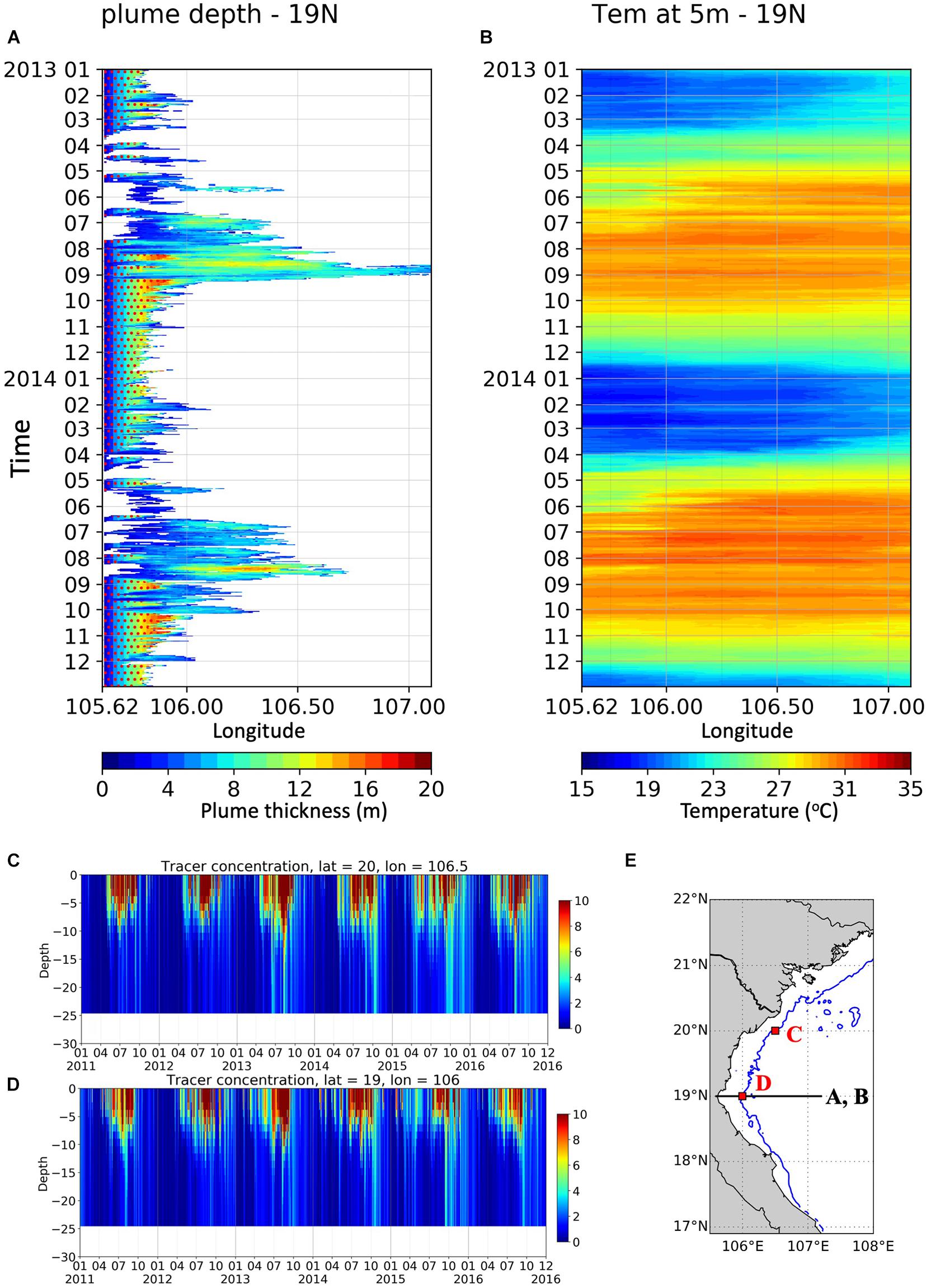
Figure 11. (A) Plume thickness (m) at 19°N section from 2013 to 2014. Red points indicate the area where the plume is present over the whole depth. (B) Temperature (°C) at 5 m at the same section as (A). (C,D) Tracer concentration over time at two coastal points. The location of the section and the points are shown in panel (E).

We estimate the export of riverine waters by computing the daily fluxes of dye concentration (for the RR and southern rivers) through three sections (Figure 2A). We then average the fluxes over the periods of the cluster to obtain a mean daily flux for each cluster. We found that the highest offshore flux (section 2) occurs in cluster 3 (∼402,000 unit/s), while the largest downcoast flux (section 1) is in cluster 2. Overall the largest exports are across section 1 in clusters 2 (473,532 unit/s) and 4 (431,408 unit/s). The flux across section 3 is much smaller in all the clusters; it is the largest (northward) in cluster 3 (76,000 unit/s).

Plume Thickness

We define the plume thickness as the maximum depth at which water is found with a tracer concentration greater than 7 unit/m³. It is computed daily. Figure 11 shows the time evolution of plume thickness and temperature at 5 m along the 19°N section. For the sake of clarity, we show years 2013 and 2014 only, representative of high and low discharge conditions respectively, but similar conclusions would be drawn for the other years (Supplementary Figure 3).

As we have seen in the previous section, from September to March, the plume is narrow and elongated along the coast due to the winter monsoon downwelling winds. During that period the plume is bottom attached, i.e., it is filling the whole water column with a thickness of the order of 10 m at 20°N and 15 m at 19°N (Figure 11A). Several factors can explain such a thickness: first the downwelling winds tend to create a convergent flow onshore; secondly the vertical mixing may be enhanced by the bottom-generated turbulence resulting from the strong coastal current (Wiseman and Garvine, 1995). Wiseman and Garvine (1995) also suggest that onshore Ekman flow may result in dense ocean water overriding buoyant plume water, therefore creating instabilities and mixing.

From May on, the monsoon changes to southwesterly wind, driving the plume northward and detaching it from the coast and from the bottom. We observe that events where the plume detaches from the coast at 19°N coincide with the temperature at the coast colder than seaward (Figure 11B). This supports the assumption that the southerly monsoon winds generate a coastal upwelling. The offshore extension of the low-temperature signal is less than 40 km. This summer upwelling was also simulated by Gao et al. (2013) for 2007, and is likely to be responsible for the detachment of the plume from the coast. When detached, the plume thickness increases from ∼4 m onshore to about 10 m seaward. Sometimes in May-August, the plume is thickening offshore to 12–15 m (Figure 11A). That deepening may be due to strong winds events that increase the mixing offshore in the upwelling region or to the increase of river discharge.

In mid-August, we observe a strong plume deepening. In 2013, the plume is still attached to the coast, contrary to 2014 (Figure 11A). This difference can be due to two reasons. Firstly, the runoff in 2013 is higher than in 2014. Secondly, the wind in 2014 is stronger than in 2013 (not shown). However, both deepening events appear to be linked with a seasonally recurrent anti-cyclonic eddy developing near 19°N, which is examined in more detail in the next section.

We also look into detail at the temporal evolution of the tracer concentration over the water column at some points near the coast (Figures 11C–E). After a peak discharge in summer, from October until November or December (depending on the year), the tracer is rapidly mixed down to the bottom (∼25 m) at a low concentration (3–5 unit/m³). Then, from January to March, the concentration gets close to zero, except for some sporadic events of a few days.

Variability of the Plume Dynamics at Daily Time Scales

The cluster analysis allowed to identify clear seasonal patterns of the plume variability, but the analysis of the plume thickness variability highlighted a strong variability at daily time scales as well. In particular, the plume is observed to spread seaward in spring and summer, which is synonymous of export of fresh water and riverine materials from the coastal zone to the interior of the GOT. Those sporadic events are represented by the 5% of plume occurrence in Figure 9. Figures 12A–C illustrates some of these events for three dates in June 2012. They show that the river waters spread within the whole basin, with a low concentration though. They extend as far east as Hainan coasts. As the forcings (wind, runoff, tides) are also strongly variable, it is not possible to disentangle their respective impacts. Besides, the plume seems to be shaped by small-scale circulation patterns over the whole shelf, suggesting that mesoscale or submesoscale activity strongly influences the horizontal transport as well as the dilution.

FIGURE 12

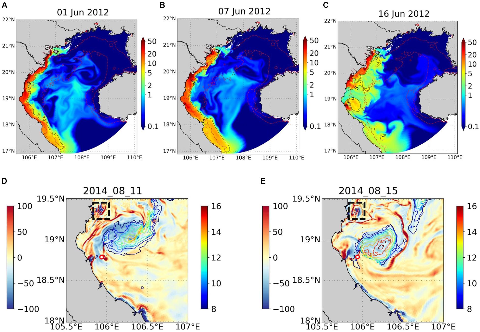
Figure 12. (A–C) Surface tracer concentration on 01 June 2012 (A), 07 June 2012 (B), and 16 June 2012 (C). (D,E) Relative surface vorticity (10⁻⁶s⁻¹) (contour fill, left color bar) and plume thickness (m) (line, right color bar) on 11 and 15 August 2014. The black box and red circle indicate the location of two islands.

In particular, at 19°N, we observe a recurrent anticyclonic eddy as mentioned in the previous section. Figures 12D,E shows the relative surface vorticity and the plume thickness on 11 and 15 August 2014. The eddy is depicted by the minimum of negative surface vorticity. It appears clearly that the plume is deepening at the center of the eddy, with a difference of thickness reaching 8 m between the edge and the center for instance on 15 August 2014. In our simulation, this eddy generally happens in August, when the wind direction is southwest, which is upwelling-favorable, and the runoff is high. Then, this eddy disappears when the coastal southward current develops again and/or the wind is not favorable anymore. Its lifetime varies from a few days to ∼15 days; its diameter is about 50 km, i.e., much larger than the first Rossby radius. There is no mention about such an eddy from the HFR analysis (Rogowski et al., 2019; Tran et al., 2021); the availability and resolution of the HFR measurements may be too limited to depict such a pattern. The formation mechanism of this eddy is unclear. The comparison with GOT_NORIV shows that most of the time, without the river, some vorticity gradients can be depicted, suggesting a weak anticyclonic structure which vanishes on a shorter time scale (for instance in 2013, 6 days in GOT_NORIV instead of 8 days in GOT_REF) (Supplementary Figure 4). The anticyclone seems strongly connected to the Lam river plume. Bottom topography may be another forcing factor. Indeed a small island is present at 106°N and is likely to influence the river flow. Both the buoyant Lam river plume and the island may generate instabilities of the coastal flow that could lead to the eddy development.

Impact of Tides

The influence of tides in shaping the far field plume is investigated by comparing the reference simulation GOT_REF with the simulation without tides (GOT_NOTIDE). We first compute the total area of the plume from all the Vietnamese rivers (including the RR). On average, the plume in GOT_REF is 5% larger than in GOT_NOTIDE, with the largest differences found in the high discharge period (not shown). Significant differences (∼10%) are observed during the summer of 2011 and 2012, with the plume being larger in the GOT_REF run; over the remaining period, the differences are weaker.

We performed a KMA analysis on the GOT_NOTIDE outputs for 4 clusters; the resulting clusters are very close to the ones from GOT_REF, both in terms of spatial structures and temporal distribution (Supplementary Figure 5). The main differences are found in clusters 3 and 4, that is during the summer monsoon and high runoff period. Without tides, the plume spreads more to the north. In cluster 4, the plume spreads a bit further to the south without tides.

Besides, of equal importance are the tidal effect on vertical mixing (already inside the estuaries) and frontal activities (Guarnieri et al., 2013). The impact of tides on the vertical mixing is investigated by comparing the tracer concentration between GOT_REF and GOT_NOTIDE (Figure 13). The tidal influence differs depending on the area: along the coast, just north of the mouth (close to ∼21°N), it is larger without tides at both surface and bottom (>4 unit/m³). Everywhere else, the bottom concentration is larger with tides (>0.5 unit/m³). At the surface, the concentration is smaller at the mouths (>4 unit/m³) and larger in the plume (0.5–1 unit/m³) in the run with tides. Over the shelf, the impact is small; in clusters 3 and 4 we observe a larger surface concentration (>0.5–1 unit/m³) in the run without tides at ∼ 107–108°E and ∼ 20°N. These differences are small but significant with regard to the concentrations in GOT_REF (Figure 13): the values are 5–50 unit/m³ (resp. 1–20 unit/m³) in the plume and 0.5–10 unit/m³ (resp. 0.1–1 unit/m³) over the shelf west of 108°E at surface and at the bottom, respectively.

FIGURE 13

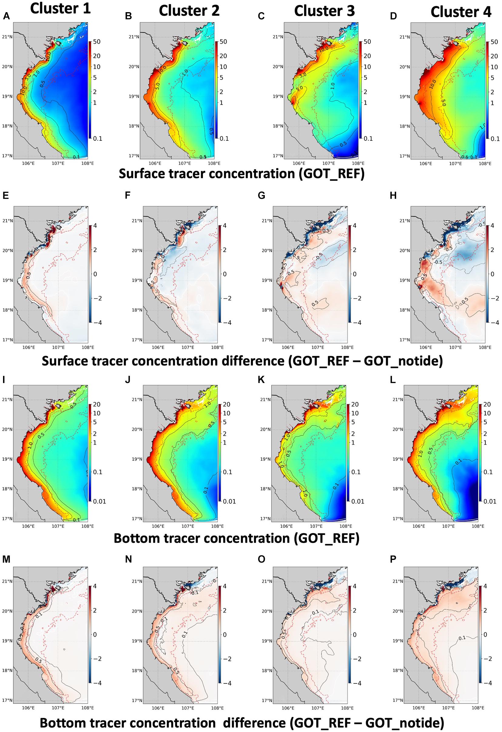
Figure 13. (A–D) Maps of mean surface tracer concentration correspond for 4 clusters. (E–H) Difference of surface tracer concentration between GOT_REF and GOT_NOTIDE correspond for 4 clusters. (I–L) Same as (A–D) but at the bottom. (M–P) Same as (E–H) but at the bottom.

We interpret the results as follows: tides enhance the vertical mixing, which explains the larger concentration at the bottom in GOT_REF. However, tides also enhance the export of riverine waters offshore at the mouth, hence the slightly larger surface concentration values in GOT_REF in the plume and the smaller concentration close to the mouth. The plume reaches the small coastal area north of the RR mouths only in the absence of tides as mentioned previously, so the surface and bottom concentrations are larger in GOT_NOTIDE.

Discussion

In this section, we summarize our findings, presenting them with paradigms found in the literature on plume dynamics (classification) or on environmental applications (receiving basins).

Classification

Several attempts have been made in the past to classify buoyant coastal runoffs with the objective of deriving general dynamical properties and to compare different plume systems. Garvine (1995) introduced the Kelvin number (K) which is defined as the ratio of the typical cross-shore scale of the buoyant runoff (usually taken as the estuary mouth width) over the local internal Rossby radius. K measures the importance of rotation: for K < 1, the influence of earth rotation on the plume dynamics is not significant and the river outflow forms energetic jets whose direction is controlled by local bathymetry and coastline (Hetland and Hsu, 2013). When K > 1, the Coriolis effect is dominant and the plume flows downcoast forming a coastal current; for large K, the downcoast flow may be insensitive to wind-driven motion in the opposite direction (Wiseman and Garvine, 1995).

Very close to the RR mouths, the internal Rossby radius is between 1.5 and 5 km. Given the typical width of the distributaries mouths in our configuration (from 0.6 to 2.5 km), the Kelvin numbers vary between 0.5 and 1. Therefore in theory, bulges could be formed and the impact of the Coriolis force should be small. Close to the mouth, the currents for each cluster do not show evidence of bulge formation. The outflow from the Cam river is very much constrained by the bathymetry and coastline. At the Van Uc and Ba Lat mouths, the outflow forms a kind of jet. In clusters 1 and 2, the plume is deflected downcoast and merges into the strong (wind-generated) coastal current (not shown). At the mouth of the Lam river, we identified daily scenes where the outflow has the shape of a bulge with a recirculating current (not shown). There the Kelvin number is estimated around 0.35, so a recurrent bulge might possibly be formed.

However, as in other delta systems, the typical length scale of the plume, and therefore the Kelvin number K, is not defined unambiguously, according to whether one considers the individual mouths or the system created by the merging plumes. Indeed, the plumes of the Red River distributaries (plus the Ma and Yen rivers) interact and merge in all clusters except cluster 3. Therefore, the overall fate of the Red River is likely to be better described by considering the system as a whole, as suggested by the ‘menagerie’ of plumes summarized by Horner-Devine et al. (2015; their Figure 5).

The Receiving Basin of Different Rivers in the GOT

As described in section “Observational Data Sets Used to Evaluate the Simulation,” the introduction of several tracers allows us to follow the pathway of different river systems: Red River, the rivers south of the RR delta (SR) and the rivers north of the RR delta (NR). This information is helpful for many practical purposes and environmental applications (e.g., contaminant dispersion, water quality). Mapping the ‘receiving basin’ of a river is a useful tool to estimate the zone of influence of dissolved or particulate terrestrial inputs, with the aim to design evaluation strategies of the coastal ocean ecological status and to build scenarios for the preservation or restoration of vulnerable areas. This is done, for instance, by Menesguen et al. (2018) in a numerical study to identify the source of eutrophication in the Bay of Biscay and the English Channel and to design a strategy of nutrient load reduction within European institutions directives framework. In this study, we define the “receiving basin” for different rivers from the passive tracer content with the same threshold as defined in section “River Plume in GOT: Identification and Variations of Area” (concentration > 7 unit/m³), but this time we apply it to each river system. The calculation is made for the high runoff/summer monsoon period (July–August–September, hereafter JAS) and for the low runoff/winter monsoon season (December–January–February, hereafter DJF) from 2011 to 2016 (Figure 14). The choice to work with ‘classical’ seasons, and not on the clusters of section “Variability of the RR Plume,” is motivated by the concern to provide maps that can be easily used by the readers of this article. For each season, the “core of the receiving basin” is the area where the plume is present at least 90% of the time, the “average receiving basin” where the plume is present at least 50% of the time, “the envelope of the receiving basin” where the plume is present at least 10% of the time. Figure 14 also shows areas where the cores/averages/envelopes of the receiving basins for two different river systems superimpose.

FIGURE 14

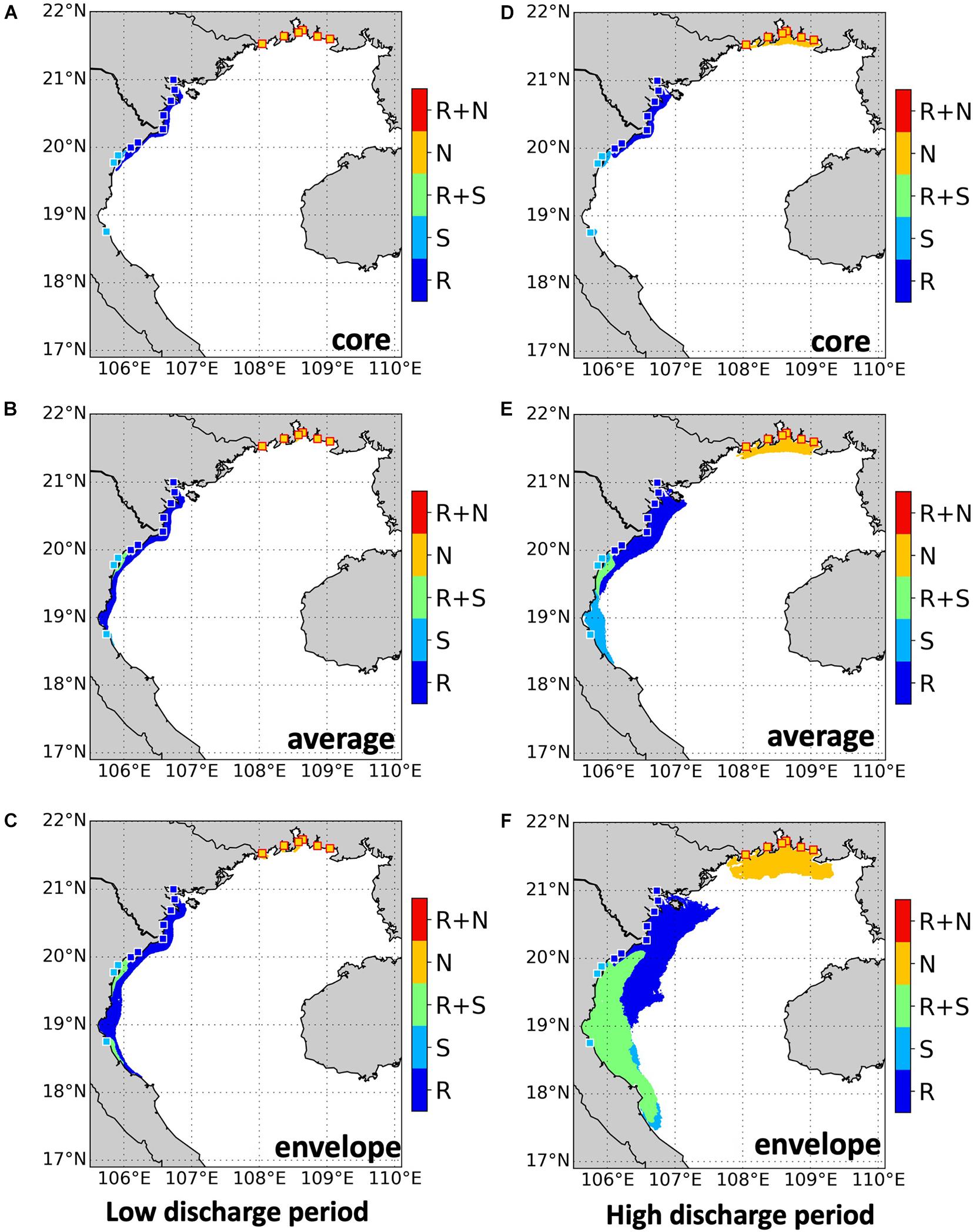
Figure 14. The “receiving basins” from different rivers. The “core of the receiving basin” is the area where the plume is present at least 90% of the time (A), the “average receiving basin” is the area where the plume is present at least 50% of the time (B), “the envelop of the receiving basin” is the area where the plume is present at least 10% of the time (C), all in low runoff period. (D–F) Same as (A–C) but in high runoff period. The location of the rivers is indicated by little boxes with the same color as the corresponding receiving basins. Explanation: (R): Red River plume, (S): plume of the rivers south of the RR delta, (N): the rivers north of the RR delta, (R+S): both R and S are present, (R+N): both R and N are present.

In the low runoff period (DJF, Figures 14A–C), the receiving basins are very narrow and elongated along the coast. While the envelope of the RR receiving basin can extend to approximately 18.2°N and mix with the plume of SR, its core appears mostly at the river mouths. In all cases, the receiving basins of NR is not detected with this choice of threshold for the tracer concentration (see below).

In the high runoff period (JAS, Figures 14D–F), the envelopes of the receiving basins of RR and SR are connected. South of 19°N, the plumes of RR and SR are fully mixed and their envelopes are indistinguishable. North of 19°N, the eastward extension of the RR envelope exceeds the one of the SR envelope and extends as eastward as 107.5°E. The receiving basin of NR appears north of 21°N but does not connect with the RR one. The average basins show different characteristics than the envelopes: while the SR influence can reach 18.3°N, the RR basin does not extend further south than 19.3°N.

In Figure 14, there is no connection between the RR and NR. However, it does not mean that they do not interact with each other. If we consider a lower threshold to identify the plume (e.g., 3 unit/m³), the envelopes of NR and RR are connected both in low and high discharge periods (not shown). This suggests that the NR waters are strongly and quickly diluted. This also means that depending on the objectives of the study, and therefore on the choice of the tracer concentration threshold, the basins will be connected or not.

As written before, the information about receiving basins can help in case of water quality monitoring or contamination leakage. This analysis leads to 2 concluding remarks. Firstly, the freshwater along the Vietnamese coasts tends to flow southward and to exit the gulf. However, the freshwater from all the rivers tends to dilute to under 7% before it leaves the domain. This means that in case of contaminant leakage, the contaminants tend to mix and affect the gulf’s water quality locally mostly. Secondly, the RR average receiving basin extends further southward and in a wider coastal strip than the SR basin during the low runoff season, while the SR basin extends further southward and further eastward (south of 19.5°N) than the RR basin during the high runoff period (Figures 14B,E). In both cases though, the RR runoff is higher than the SR runoff. These contrasted situations highlight the importance of wind and coastal circulation on shaping the receiving basin and consequently, on the fate of terrestrial inputs depending on their origin (SR or RR rivers systems).

Conclusion

We presented a comprehensive study of the plume formed by the waters from the Red River and three nearby rivers in the GOT using numerical simulation, in a realistic high-resolution configuration over the period 2011–2016. Compared to various observational data, the model shows good results. We then compare several methods to identify the river plume in the study area. We found that identification through passive (dye-like) tracers is preferable since it allows to distinguish the runoff influence from the precipitation one and to distinguish the runoff from different rivers as well. The runoff shows large seasonal and interannual variability. It usually reaches the highest value in August and lowest in February, in phase with the monsoon system. At the surface, the plume area shows similar variations. However, the plume area reaches its peak in September, which is about 1 month later than the peak of runoff.

To identify the main spatial patterns of variability, we apply a clustering method to daily scenes of the model outputs where the plume is defined from the tracer concentration (>7 arbitrary unit/m³). The cluster analysis identifies the plume regimes and their period of occurrence without having to pre-define these periods as one would do when computing seasonal averages for instance. Besides it allows identifying transition regimes (e.g., cluster 2).

The plume pattern of the first cluster is characteristic of the November–March period: the plume is narrow and contained within the inner shelf (bottom depth < 20 m), due to low runoff and downwelling wind (winter monsoon) with an intense downcoast current. The second pattern is mainly observed in the transition period of the monsoon (April, May, October) and is wider than the first pattern; both the relaxation of the winter monsoon and the weaker coastal current allow the plume to spread further offshore than in cluster 1. The third pattern occurs when the summer monsoon is the strongest and the runoff increases. The wind is upwelling favorable; the plumes are advected northward and detach locally from the coast. It is the only pattern where the plumes from the different rivers are disconnected. The final pattern coincides with the highest runoff period and the summer monsoon relaxation. The plumes are connected again in a pool of low salinity waters with the largest coverage, spreading both offshore and southward. Overall, we found that this hydrological system with multiple source points and a strong seasonal variability of along-shore wind is similar to the one for instance described by Kourafalou et al. (1996) in the Southern Atlantic Bight along the US coast.

The vertical variability of the plume is examined as well. In winter, the plume is usually mixed over the whole water depth. When the summer monsoon arrives at the end of March, the plume starts to detach from the bottom and spreads offshore as a surface buoyant layer. The plume can detach from the coast near 19°N when a coastal upwelling develops. It may deepen offshore also. In particular, the plume is strongly deepened in the middle of August when trapped in a recurrent eddy near 19°N.

The cluster analysis therefore evidenced at least three regimes. In winter regime, the plumes of all the Vietnamese rivers are connected in a well-mixed freshwater strip which is contained to the coast; the downcoast current is likely to act like a barrier preventing exchanges of riverine water and material cross-shore toward the center of the gulf. In early summer, the upwelling winds lead to a reverse circulation, where the plumes are advected northward and slightly offshore; the plumes are partly disconnected from each other. In the late summer regime, the wind relaxes and the large amount of freshwater due to the annual runoff peak spreads at the surface, reaching the maximal offshore and southward extension.

The impact of tides on the shape of the plume has been explored using a dedicated simulation without tides; we found that the general shape of the plume is not significantly influenced by tides, except in the Ha Long Bay area during the high runoff period (clusters 3 and 4). The main forcings of the far-field plume are the wind and basin-scale circulation. However, tides impact the vertical structure of the plume: they enhance the vertical mixing hence the riverine water concentration in the bottom layer. They also lead to a larger export offshore or the riverine water at the surface close to the mouth during the high discharge season. The influence of tides is obviously not limited to the far field; first, tides determine the buoyancy of the river water entering the ocean. Then, in the near and mid-field area, the bottom friction induced by tides is likely to impact the local dynamics and mixing, therefore influencing the plume properties in the far-field as well. An in-depth analysis of the tidal processes, of the tides-river flow interactions and of their impact on the velocity, shear and stratification in the estuaries and at the mouths was beyond the scope of this paper. It will be the topic of a future study aimed at better understanding the shape and dynamics of the outflow in the near and mid fields. The dynamics at the mouth is also highly important for sediment dynamics close to the mouth area.

Small-scale patterns of the coastal circulation, such as the recurrent eddy observed at 19°N in August, are also involved in the dilution and fate of the riverine water in the ocean. Submesoscale features due to instabilities within the plume or at the fronts may also develop and influence the mixing as found in other systems (e.g., Horner-Devine et al., 2015; Ayouche et al., 2021 this issue). Such small-scale processes should be examined in dedicated studies.

At last, this study provides some reference information about the river plume variability, showing in particular the role of the wind. In such a context, ensemble simulations will be useful to assess the sensitivity of our results due to the uncertainty of the forcing conditions (wind and runoff).

Data Availability Statement

The raw data supporting the conclusions of this article (i.e., the model simulations) will be made available by the authors without undue reservation.

Author Contributions

TuN-D, NA, PM, and PDM-F contributed to the conception and scientific design of the study. PM provided the model. VP, MH, TD, and PM developed the previous GOT configuration used for this analysis. MT provided the HFR data. TuN-D, NA, and FT performed most of the analyses. TuN-D wrote the first draft of the manuscript. NA wrote sections of the manuscript. All authors actively contributed to manuscript revision, read, and approved the submitted version.

Funding

TuN-D Ph.D. thesis is funded by the “Programme d’Excellence” of the French Embassy of Vietnam and by IRD ARTS program. This work is a contribution to the LMI LOTUS project (http://lotus.usth.edu.vn) and to the SWOT COCTO-FO project funded by CNES (French Spatial Agency). This work has used HPC resources from CALMIP/France (grant 2020-p1119) and HILO at the University of Science and Technology of Hanoi (USTH). Support from IRD, CNES, CNRS, and USTH is gratefully acknowledged.

Conflict of Interest

The authors declare that the research was conducted in the absence of any commercial or financial relationships that could be construed as a potential conflict of interest.

Publisher’s Note

All claims expressed in this article are solely those of the authors and do not necessarily represent those of their affiliated organizations, or those of the publisher, the editors and the reviewers. Any product that may be evaluated in this article, or claim that may be made by its manufacturer, is not guaranteed or endorsed by the publisher.

Acknowledgments

CFO CTD data used in this study was collected by the Vietnam Center for Oceanography (CFO, VASI) in the framework of the United States–Vietnam collaboration project: “Gulf of Tonkin Circulation study” (NICOP N62909-15-1-2018), financed by the Office of Naval Research (ONR). The VITEL (VIetnam TELédétection remote sensing) campaign has been funded by CNES; we are grateful to S. Ouillon for providing the T/S data. The historical tidal gauges dataset stems from the International Hydrographic Organization (https://www.iho.int/, last access: November 2, 2019) and is available upon request at https://www.admiralty.co.uk/ukho/tidal-harmonics (last access: November 2, 2019). The altimetric tidal constituents were provided to us by F. Lyard (LEGOS). We also acknowledge F. Lyard for the use of his code to compute the Rossby Radius and for his expertise on the model’s bathymetry field. This study has been conducted using ECMWF product (www.ecmwf.int) and E.U. Copernicus Marine Service Information (product: GLOBAL_ANALYSIS_FORECAST_PHY_001_024, available at https://resources.marine.copernicus.eu/?option=com_csw&view=details&product_id=GLOBAL_ANALYSIS_FORECAST_PHY_001_024). Many thanks to C. Nguyen and D. Gazen for the help with the model and computing facilities at LAERO (Toulouse). The SYMPHONIE code and the code to compute the Rossby radius are distributed by the SIROCCO French national service website (https://sirocco.obs-mip.fr/), hosted by the Observatoire Midi-Pyrénées, Toulouse, France.

Supplementary Material

The Supplementary Material for this article can be found online at: https://www.frontiersin.org/articles/10.3389/fmars.2021.772139/full#supplementary-material

Footnotes

1. ^ https://www.iho.int/

References

Ayouche, A., Charria, G., Carton, X., Ayoub, N., and Theetten, S. (2021). Non-linear processes in the Gironde river plume (North-East Atlantic): instabilities and mixing. Front. Mar. Sci. 8:701773. doi: 10.3389/fmars.2021.701773

CrossRef Full Text | Google Scholar

Bentsen, M., Evensen, G., Drange, H., and Jenkins, A. D. (1999). Coordinate transformation on a sphere using conformal mapping. Mon. Weather Rev. 127, 2733–2740.

Google Scholar

Blumberg, A. F., and Mellor, G. L. (1987). “A description of a three–dimensional coastal ocean circulation model,” in Three-Dimensional Coastal Ocean Models, ed. N. S. Heaps (Washington, DC: American Geophysical Union), doi: 10.1029/CO004p0001

CrossRef Full Text | Google Scholar

Burla, M., Baptista, A. M., Zhang, Y., and Frolov, S. (2010). Seasonal and interannual variability of the Columbia river plume: a perspective enabled by multiyear simulation databases. J. Geophys. Res. 115:C00B16. doi: 10.1029/2008JC004964

CrossRef Full Text | Google Scholar

Chelton, D. B., deSzoeke, R. A., Schlax, M. G., El Naggar, K., and Siwertz, N. (1998). Geographical variability of the first baroclinic rossby radius of deformation. J. Phys. Oceanogr. 28, 433–460.

Google Scholar

Chen, Z., Gong, W., Cai, H., Chen, Y., and Zhang, H. (2017). Dispersal of the Pearl river plume over continental shelf in summer. Estuar. Coast. Shelf Sci. 194, 252–262. doi: 10.1016/j.ecss.2017.06.025

CrossRef Full Text | Google Scholar

Csanady, G. T. (1982). Circulation in the Coastal Ocean. Dordrecht: Springer, 281. doi: 10.1007/978-94-017-1041-1

CrossRef Full Text | Google Scholar

Damien, P., Bosse, A., Testor, P., Marsaleix, P., and Estournel, C. (2017). Modeling postconvective submesoscale coherent vortices in the Northwestern Mediterranean Sea. J. Geophys. Res. Oceans 122, 9937–9961. doi: 10.1002/2016JC012114

CrossRef Full Text | Google Scholar

Ding, Y., Chen, C., Beardsley, R. C., Bao, X., Shi, M., Zhang, Y., et al. (2013). Observational and model studies of the circulation in the Gulf of Tonkin, South China Sea. J. Geophys. Res. Oceans 118, 6495–6510. doi: 10.1002/2013JC009455

CrossRef Full Text | Google Scholar

Falcieri, F. M., Benetazzo, A., Sclavo, M., Russo, A., and Carniel, S. (2014). Po river plume pattern variability investigated from model data. Cont. Shelf Res. 87, 84–95. doi: 10.1016/j.csr.2013.11.001

CrossRef Full Text | Google Scholar

Gao, J., Shi, M., Chen, B., Guo, P., and Zhao, D. (2014). Responses of the circulation and water mass in the Beibu Gulf to the seasonal forcing regimes. Acta Oceanol. Sin. 33, 1–11.

Google Scholar

Gao, J., Xue, H., Chai, F., and Shi, M. (2013). Modeling the circulation in the Gulf of Tonkin, South China Sea topical collection on the 4th international workshop on modelling the ocean in Yokohama, Japan 21–24 May 2012. Ocean Dyn. 63, 979–993. doi: 10.1007/s10236-013-0636-y

CrossRef Full Text | Google Scholar

Garvine, R. W. (1995). A dynamical system for classifying buoyant coastal runoffs. Cont. Shelf Res. 15, 1585–1596.

Google Scholar

Greenberg, D. A., Dupont, F., Lyard, F. H., Lynch, D. R., and Werner, F. E. (2007). Resolution issues in numerical models of oceanic and coastal circulation. Cont. Shelf Res. 27, 1317–1343. doi: 10.1016/j.csr.2007.01.023

CrossRef Full Text | Google Scholar

Guarnieri, A., Pinardi, N., Oddo, P., Bortoluzzi, G., and Ravaioli, M. (2013). Impact of tides in a baroclinic circulation model of the Adriatic Sea. J. Geophys. Res. Oceans 118, 166–183. doi: 10.1029/2012JC007921

CrossRef Full Text | Google Scholar

Hansen, D. V., and Rattray, M. (1966). New dimensions in estuary classification. Limnol. Oceanogr. 11, 319–326. doi: 10.4319/lo.1966.11.3.0319

CrossRef Full Text | Google Scholar

Hastie, T., Tsbshirani, R., and Friedman, J. (2001). The Elements of Statistical Learning: Data Mining, Inference, and Prediction. New York, NY: Springer, 533.

Google Scholar

Hetland, R. D., and Hsu, T.-J. (2013). “Freshwater and sediment dispersal in large river plumes,” in Biogeochemical Dynamics at Large River–Coastal Interfaces: Linkages with Global Climate Change, eds T. S. Bianchi, M. A. Allison, and W.-J. Cai (New York, NY: Springer), 55–85.

Google Scholar

Horner-Devine, A. R., Hetland, R. D., and MacDonald, D. G. (2015). Mixing and transport in coastal river plumes. Annu. Rev. Fluid Mech. 47, 569–594. doi: 10.1146/annurev-fluid-010313-141408

CrossRef Full Text | Google Scholar

Kourafalou, V. H., Lee, T. N., Oey, L.-Y., and Wang, J. D. (1996). The fate of river runoff on the continental shelf: 2. Transport of coastal low–salinity waters under realistic wind and tidal forcing. J. Geophys. Res. 101, 3435–3455. doi: 10.1029/95JC03025

CrossRef Full Text | Google Scholar

Large, W. G., and Yeager, S. (2004). Diurnal to Decadal Global Forcing for Ocean and Sea–Ice Models: The Data Sets and Flux Climatologies, NCAR Technical Note, NCAR/TN-460+STR. Boulder, CO: National Center for Atmospheric Research. doi: 10.5065/D6KK98Q6

CrossRef Full Text | Google Scholar

Liu, Y., MacCready, P., and Hickey, B. M. (2009). Columbia river plume patterns in summer 2004 as revealed by a hindcast coastal ocean circulation model. Geophys. Res. Lett. 36:L02601. doi: 10.1029/2008GL036447

CrossRef Full Text | Google Scholar

Lyard, F. H., Allain, D. J., Cancet, M., Carrère, L., and Picot, N. (2021). FES2014 global ocean tide atlas: design and performance. Ocean Sci. 17, 615–649. doi: 10.5194/os-17-615-2021

CrossRef Full Text | Google Scholar

MacCready, P., Banas, N. S., Hickey, B. M., Dever, E. P., and Liu, Y. (2009). A model study of tide– and wind–induced mixing in the Columbia river estuary and plume. Cont. Shelf Res. 29, 278–291. doi: 10.1016/j.csr.2008.03.015

CrossRef Full Text | Google Scholar

Maraldi, C., Chanut, J., Levier, B., Ayoub, N., De Mey, P., Reffray, G., et al. (2013). NEMO on the shelf: assessment of the Iberia–Biscay–Ireland configuration. Ocean Sci. 9, 745–771. doi: 10.5194/os-9-745-2013

CrossRef Full Text | Google Scholar

Marsaleix, P., Auclair, F., and Estournel, C. (2006). Considerations on open boundary conditions for regional and coastal ocean models. J. Atmos. Ocean. Technol. 23, 1604–1613. doi: 10.1175/JTECH1930.1

CrossRef Full Text | Google Scholar

Marsaleix, P., Auclair, F., Floor, J. W., Herrmann, M. J., Estournel, C., Pairaud, I., et al. (2008). Energy conservation issues in sigma–coordinate free–surface ocean models. Ocean Model. 20, 61–89. doi: 10.1016/j.ocemod.2007.07.005

CrossRef Full Text | Google Scholar

Menesguen, A., Dussauze, M., and Dumas, F. (2018). Designing optimal scenarios of nutrient loading reduction in a WFD/MSFD perspective by using passive tracers in a biogeochemical–3D model of the English Channel/Bay of Biscay area. Ocean Coast. Manage. 163, 37–53. doi: 10.1016/j.ocecoaman.2018.06.005

CrossRef Full Text | Google Scholar

Michaud, H., Marsaleix, P., Leredde, Y., Estournel, C., Bourrin, F., Lyard, F., et al. (2012). Three–dimensional modelling of wave–induced current from the surf zone to the inner shelf. Ocean Sci. 8, 657–681. doi: 10.5194/os-8-657-2012

CrossRef Full Text | Google Scholar

Neumann, L. E., Šimůnek, J., and Cook, F. J. (2011). Implementation of quadratic upstream interpolation schemes for solute transport into HYDRUS–1D. Environ. Model. Softw. 26:11. doi: 10.1016/j.envsoft.2011.05.010

CrossRef Full Text | Google Scholar

Nguyen, N. M., Marchesiello, P., Lyard, F., Ouillon, S., Cambon, G., Allain, D., et al. (2014). Tidal characteristics of the Gulf of Tonkin. Cont. Shelf Res. 91, 37–56. doi: 10.1016/j.csr.2014.08.003

CrossRef Full Text | Google Scholar

Nguyen Thi Hien, A., Vu Minh Cat, B., and Roberto Ranzi, C. (2020). “Upstream effects on salinity dynamics in the Red River Delta,” in APAC 2019, eds N. Trung Viet, D. Xiping, and T. Thanh Tung (Singapore: Springer), 1439–1443.

Google Scholar

Nugroho, D. (2017). The Tides in a General Circulation Model in the Indonesian Seas. Ph.D. thesis. Toulouse: Univ. Paul Sabatier 3.

Google Scholar

Otero, P., Ruiz-Villarreal, M., and Peliz, A. (2008). Variability of river plumes off Northwest Iberia in response to wind events. J. Mar. Syst. 72, 238–255. doi: 10.1016/j.jmarsys.2007.05.016

CrossRef Full Text | Google Scholar

Ouillon, S. (2014). VITEL–NORTH Cruise, RV Alis. doi: 10.17600/14004100

PubMed Abstract | CrossRef Full Text | Google Scholar

Pairaud, I. L., Lyard, F., Auclair, F., Letellier, T., and Marsaleix, P. (2008). Dynamics of the semi–diurnal and quarter–diurnal internal tides in the Bay of Biscay. Part 1: barotropic tides. Cont. Shelf Res. 28, 1294–1315. doi: 10.1016/j.csr.2008.03.004

CrossRef Full Text | Google Scholar

Pedregosa, F., Varoquaux, G., Gramfort, A., Michel, V., Thirion, B., Grisel, O., et al. (2011). Scikit–learn: machine learning in python. J. Mach. Learn. Res. 12, 2825–2830.

Google Scholar

Piton, V., Herrmann, M., Lyard, F., Marsaleix, P., Duhaut, T., Allain, D., et al. (2020). Sensitivity study on the main tidal constituents of the Gulf of Tonkin by using the frequency–domain tidal solver in T–UGOm. Geosci. Model Dev. 13, 1583–1607. doi: 10.5194/gmd-13-1583-2020

CrossRef Full Text | Google Scholar

Piton, V., Herrmann, M., Marsaleix, P., Duhaut, T., Ngoc, T. B., Tran, M. C., et al. (2021). Influence of winds, geostrophy and typhoons on the seasonal variability of the circulation in the Gulf of Tonkin: a high–resolution 3D regional modeling study. Reg. Stud. Mar. Sci. 45:101849. doi: 10.1016/j.rsma.2021.101849

CrossRef Full Text | Google Scholar

Reffray, G., Fraunié, P., and Marsaleix, P. (2004). Secondary flows induced by wind forcing in the Rhône region of freshwater influence. Ocean Dyn. 54, 179–196. doi: 10.1007/s10236-003-0079-y

CrossRef Full Text | Google Scholar

Rogowski, P., Zavala-Garay, J., Shearman, K., Terrill, E., Wilkin, J., and Tran, H. L. (2019). Air-sea-land forcing in the Gulf of Tonkin: assessing seasonal variability using modern tools. Oceanography 32, 150–161. doi: 10.5670/oceanog.2019.223

CrossRef Full Text | Google Scholar

Shi, M., Chen, C., Xu, Q., Lin, H., Liu, G., Wang, H., et al. (2002). The role of Qiongzhou Strait in the seasonal variation of the South China Sea circulation. J. Phys. Oceanogr. 32, 103–121. doi: 10.1175/1520-04852002032<0103:TROQSI<2.0.CO;2

CrossRef Full Text | Google Scholar

Solabarrieta, L., Rubio, A., Cárdenas, M., Castanedo, S., Esnaola, G., Méndez, F. J., et al. (2015). Probabilistic relationships between wind and surface water circulation patterns in the SE Bay of Biscay. Ocean Dyn. 65, 1289–1303. doi: 10.1007/s10236-015-0871-5

CrossRef Full Text | Google Scholar

Sonnewald, M., Wunsch, C., and Heimbach, P. (2019). Unsupervised learning reveals geography of global ocean dynamical regions. Earth Space Sci. 6, 784–794. doi: 10.1029/2018EA000519

PubMed Abstract | CrossRef Full Text | Google Scholar

Sutton, W. R., Srivastava, J. P., Rosegrant, M., Thurlow, J., and Sebastian, L. (2019). Striking a Balance, Managing El Niòo and la Niòa in Vietnam Agriculture, RepNo 132068. Washington, DC: World Bank.

Google Scholar

Toublanc, F., Ayoub, N. K., Lyard, F., Marsaleix, P., and Allain, D. J. (2018). Tidal downscaling from the open ocean to the coast: a new approach applied to the Bay of Biscay. Ocean Model. 124, 16–32. doi: 10.1016/j.ocemod.2018.02.001

CrossRef Full Text | Google Scholar

Tran, M. C., Sentchev, A., and Nguyen, K. C. (2021). Multi-scale variability of circulation in the Gulf of Tonkin from remote sensing of surface currents by high-frequency radars. Ocean Dyn. 71, 175–194. doi: 10.1007/s10236-020-01440-x

CrossRef Full Text | Google Scholar

Vaz, N., Rodrigues, J. G., Mateus, M., Franz, G., Campuzano, F., Neves, R., et al. (2018). Subtidal variability of the Tagus river plume in winter 2013. Sci. Total Environ. 627, 1353–1362. doi: 10.1016/j.scitotenv.2018.01.325

PubMed Abstract | CrossRef Full Text | Google Scholar

Vinh, V. D., Ouillon, S., Thanh, T. D., and Chu, L. V. (2014). Impact of the Hoa Binh dam (Vietnam) on water and sediment budgets in the Red river basin and delta. Hydrol. Earth Syst. Sci. 18, 3987–4005. doi: 10.5194/hess-18-3987-2014

CrossRef Full Text | Google Scholar

Vlasenko, V., Stashchuk, N., and McEwan, R. (2013). High–resolution modelling of a large–scale river plume. Ocean Dyn. 63, 1307–1320. doi: 10.1007/s10236-013-0653-x

CrossRef Full Text | Google Scholar

Wang, Y., Xue, H., Chai, F., Chao, Y., and Farrara, J. (2014). A model study of the Copper river plume and its effects on the northern Gulf of Alaska topical collection on the 5th International Workshop on Modelling the Ocean (IWMO) in Bergen, Norway 17–20 June 2013. Ocean Dyn. 64, 241–258. doi: 10.1007/s10236-013-0684-3

CrossRef Full Text | Google Scholar

Wiseman, W. J., and Garvine, R. W. (1995). Plumes and coastal currents near large river mouths. Estuaries 18:509. doi: 10.2307/1352368

CrossRef Full Text | Google Scholar

Wu, D., Wang, Y., Lin, X., and Yang, J. (2008). On the mechanism of the cyclonic circulation in the Gulf of Tonkin in the summer. J. Geophys. Res. Oceans 113, 2–11. doi: 10.1029/2007JC004208

CrossRef Full Text | Google Scholar

Yankovsky, A. E., and Chapman, D. C. (1997). A simple theory for the fate of buoyant coastal runoffs. J. Phys. Oceanogr. 27, 1386–1401.

Google Scholar