Turnover Time of the East Sea (Sea of Japan) Meridional Overturning Circulation

The East Sea (ES; Sea of Japan) meridional overturning circulation (MOC) serves as a crucial mechanism for the transportation of dissolved, colloidal, and suspended particulate matters, including pollutants, on the surface to deep waters via thermohaline circulation. Therefore, understanding the structure of the ES MOC is critical for characterizing its temporal and spatial distribution. Numerous studies have estimated these parameters indirectly using chemical tracers, severely limiting the accuracy of the results. In this study, we provide a method for directly estimating the turnover times of the ES MOC using the stream functions calculated from HYbrid Coordinate Ocean Model (HYCOM) reanalysis data by averaging the flow pattern in the meridional 2-D plane. Because the flow pattern is not consistent but various over time, three cases of stream function fields were computed over a 20-year period. The turnover time was estimated by calculating the time required for water particles to circulate along the streamlines. In the cases of multiple (two or three) convection cells, we considered all possible scenarios of the exchange of water particles between adjacent cells, so that they circulated over those cells until finally returning to the original position and completing the journey on the ES MOC. Three different cell cases were tested, and each case had different water particle exchange scenarios. The resulting turnover times were 17.91–58.59 years, 26.41–37.28 years, and 8.68–45.44 years for the mean, deep, and shallow convection cases, respectively. The maximum turnover time, namely 58.59 years, was obtained when circulating the water particle over all three cells, and it was approximately half of that estimated by the chemical tracers in previous studies (∼100 years). This underestimation arose because the streamlines and water particle movement were not calculated in the shallow (<300 m) and deep areas (>3,000 m) in this study. Regardless, the results of this study provide insight into the ES MOC dynamics and indicate that the traditional chemical turnover time represents only one of the various turnover scenarios that could exist in the ES.

Introduction

The East Sea (ES; Sea of Japan) is a semi-enclosed marginal sea connected to the North Pacific, East China Sea, Yellow Sea, and Sea of Okhotsk via relatively narrow and shallow straits such as the Korea/Tsushima, Tsugaru, Soya, and Tatarsky Straits. These straits result in the active exchange of seawater with adjacent oceans and seas from the surface to depths of ∼300 m (Figure 1; Chang et al., 2016; Han et al., 2020). In addition, the sea surface atmospheric and oceanic conditions of the ES result in strong ventilation of deep dissolved oxygen in this small deep basin compared to the weak ventilation in the Pacific Ocean (Kim et al., 2001; Talley et al., 2006; Yoon et al., 2018; Han et al., 2020). This ventilation process occurs in intrinsic internal circulations in both horizontal and vertical directions and is related to meridional overturning circulation (MOC; Wunsch, 2002; Stouffer et al., 2006; Han et al., 2020). Horizontally, in the upper part of the ES MOC, currents such as the East Korea Warm Current and the Tsushima Warm Current are generated to carry warm and saline water to the north, whereas the North Korea Cold Current transports cold and less saline water to the south (Cho and Kim, 1998; Kim and Kim, 1999; Yoshikawa et al., 1999; Yun et al., 2004; Kim et al., 2006; Min and Kim, 2006; Park and Lim, 2018). Moreover, the ES MOC is developed vertically to carry dissolved, colloidal, and suspended particulate matters together with other bio-reactive elements between the surface and deep waters (Kim and Kim, 2012; Han et al., 2020). These matters can contain fractions of pollution from the surface water, which are then transported to deeper waters via the ES MOC; thus, a precise understanding of the spatial (MOC paths) and temporal (turnover time) structure of the ES MOC is crucial (Kawamura et al., 2007). In addition, the ES is often referred to as a “miniature ocean” because it has a circulation pattern similar to that of the global ocean (Ichiye, 1984; Kim et al., 2002; Talley et al., 2003). Therefore, studies on the ES MOC process and structure may provide a foundation for a better understanding of the global MOC that occurs at a much slower time scale.

FIGURE 1

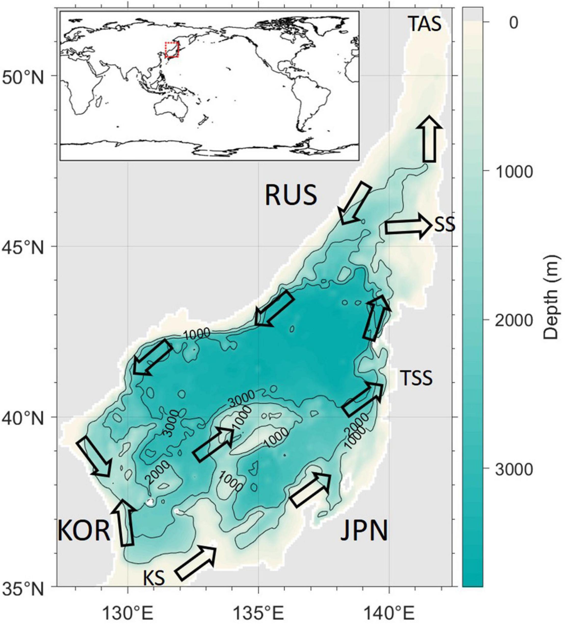
Figure 1. Map of the East Sea (ES; Sea of Japan). Open arrows represent major surface currents. The iso-depth interval is 1,000 m and land is shaded in light gray. KOR, RUS, and JPN indicate Korea, Russia, and Japan, respectively. KS, TSS, SS, and TAS denote Korea/Tsushima, Tsugaru, Soya, and Tatarsky straits, respectively. The ES is represented by a red dotted rectangle on the world map (upper left). Latitudinal sections in Figures 2–9 are zonally integrated sections in the ES because the ES MOC was calculated with zonally integrated values.

FIGURE 2

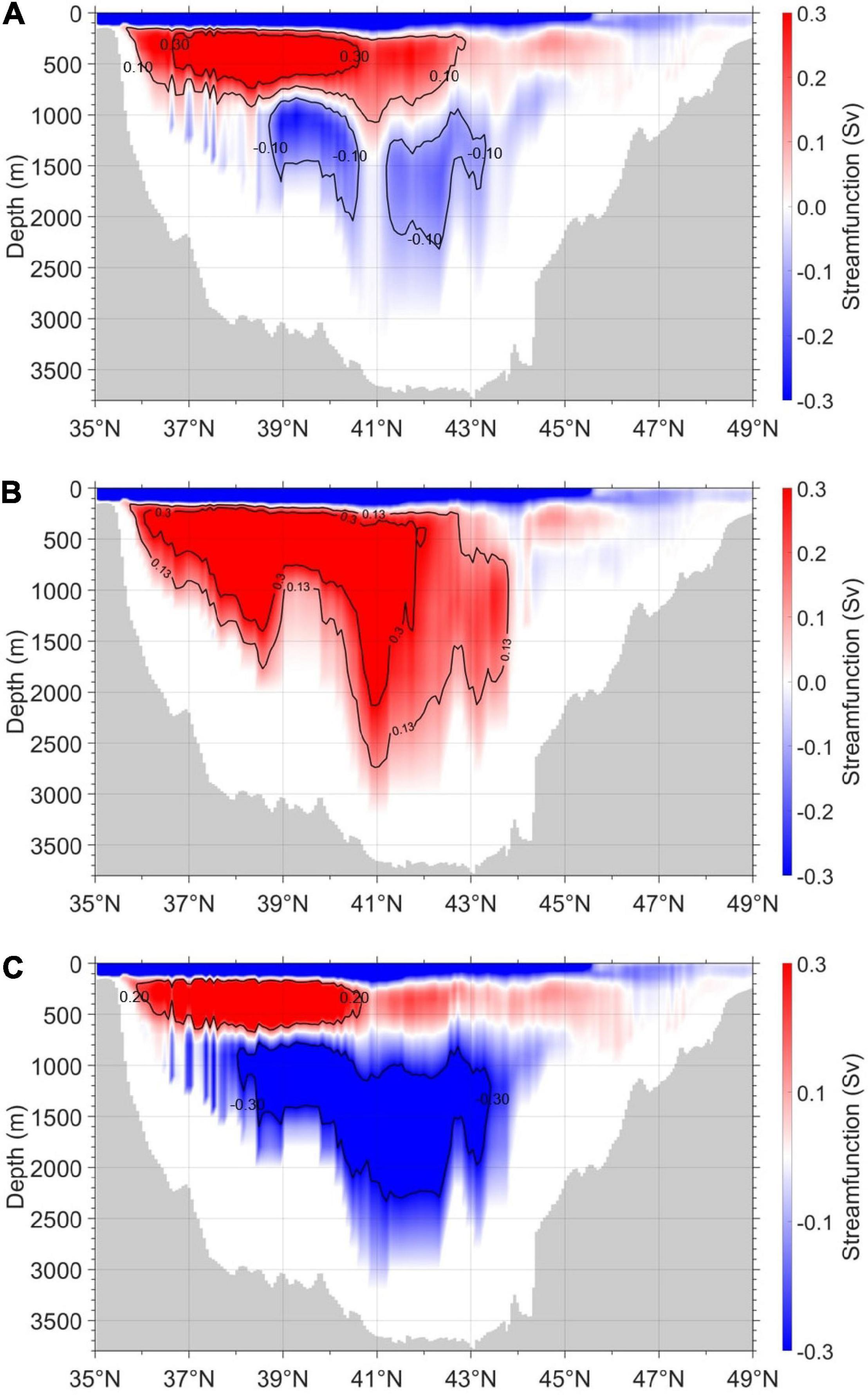
Figure 2. (A) Mean convection (1993–2012), (B) deep convection, (1993, 2002, 2004–2009) and (C) shallow convection (1996–2001 and 2010–2012) cases in the meridional overturning stream functions. The contour intervals are (A) −0.1, 0.1, and 0.3 Sv; (B) 0.13 and 0.3 Sv; and (C) −0.3 and 0.2 Sv, respectively.

FIGURE 3

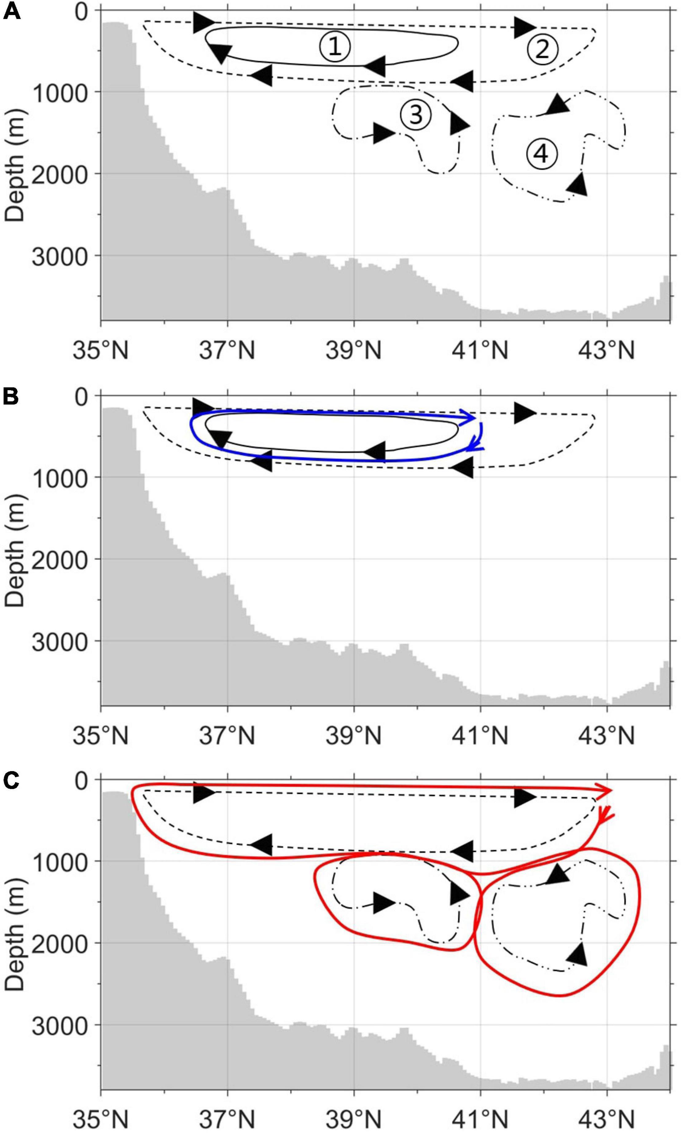
Figure 3. (A) Streamlines of 0.3 Sv (①: solid line), 0.1 Sv (②: dashed line), and −0.1 Sv (③: left dot-dashed line and ④: right dot-dot-dashed line) for the mean convection case in the meridional overturning stream function from Figure 2A. Individual turnover times are ① 17.91, ② 18.04, ③ 16.95, and ④ 23.6 years, respectively. (B) Turnover times of upper cells from ∼300 to ∼700 m and from ∼300 to ∼900 m: ① 17.91 and ② 18.04 years, respectively. (C) Turnover times of upper and lower cells: (②+③) 34.99 years, (②+④) 41.64 years, and (②+③+④) 58.59 years, respectively.

FIGURE 4

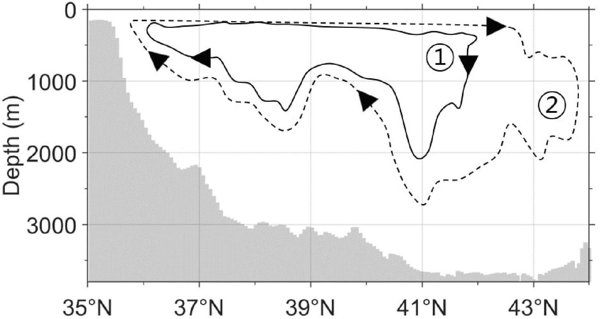
Figure 4. Streamlines of 0.3 Sv (①: solid line) and 0.13 Sv (②: dashed line) for the deep convection case in the meridional overturning stream function from Figure 2B. Individual turnover times are ① 26.41 years and ② 37.28 years, respectively.

FIGURE 5

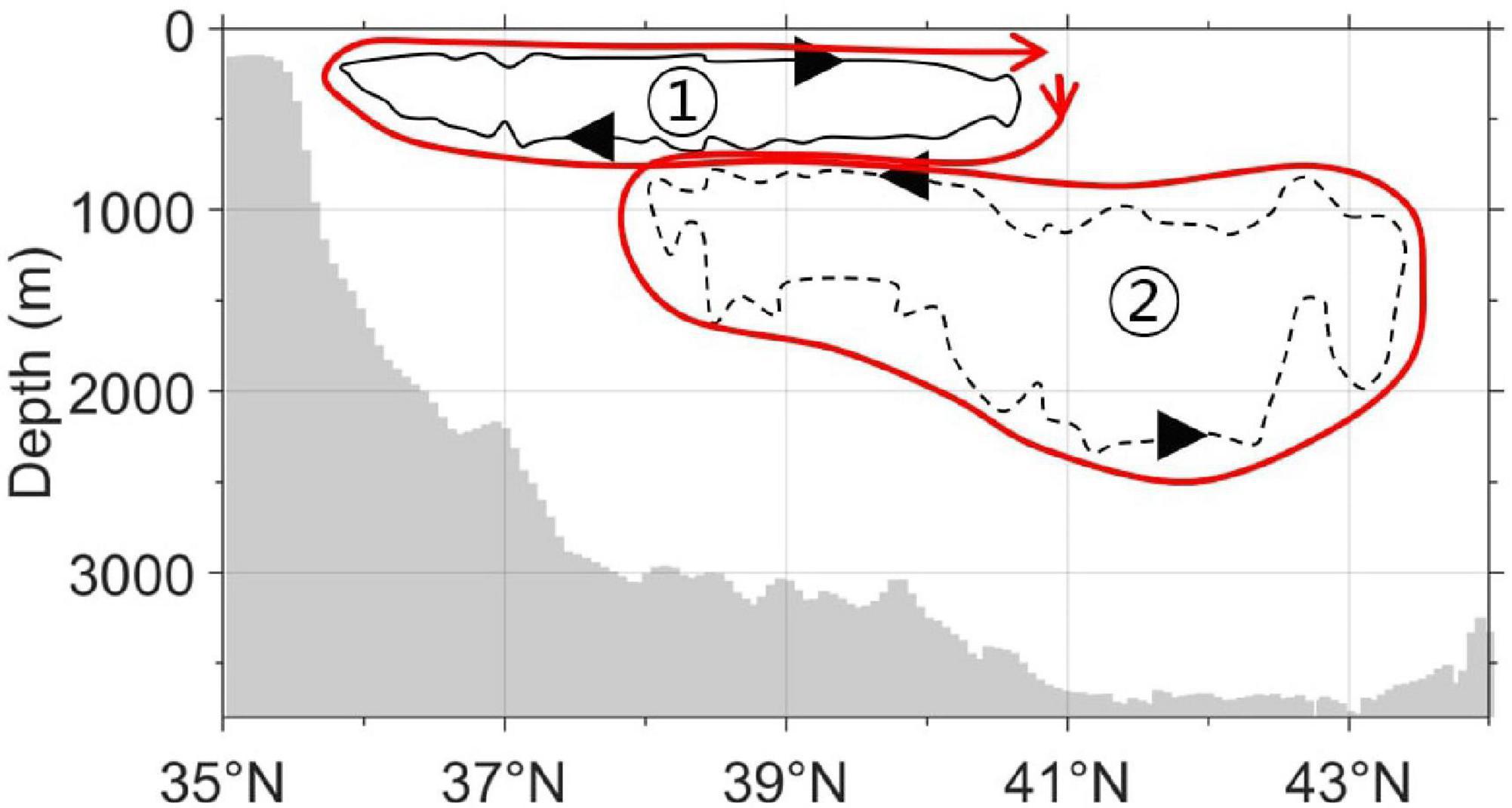
Figure 5. Streamlines of 0.2 Sv (①: solid line) and −0.3 Sv (②: dashed line) for the shallow convection case in the meridional overturning stream function from Figure 2C. Turnover times are ① 8.68 years, ② 36.76 years, and ①+② 45.44 years, respectively.

FIGURE 6

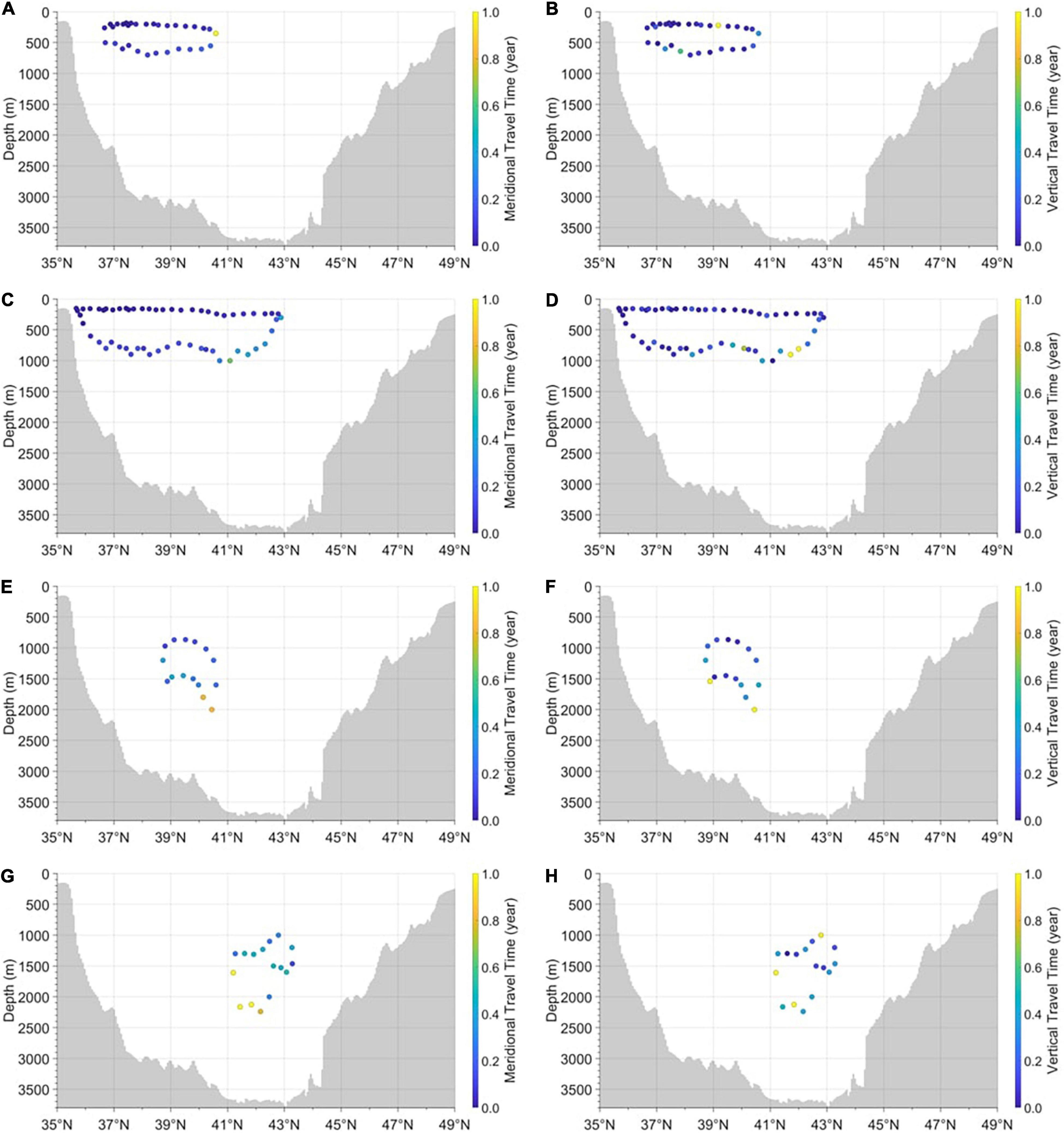
Figure 6. Meridional and vertical travel times of 0.3 Sv (A,B), 0.1 Sv (C,D), and −0.1 Sv (E–H) streamlines for the mean convection case in the meridional overturning stream function. Turnover times of the 0.3 Sv (A,B), 0.1 Sv (C,D), −0.1 Sv (E,F), and −0.1 Sv (G,H) streamlines are 17.91 years (= 3.62 + 14.29), 18.04 years (= 6.52 + 11.52), 23.60 years (= 4.83 + 18.77), and 16.95 years (= 9.81 + 7.14), respectively.

FIGURE 7

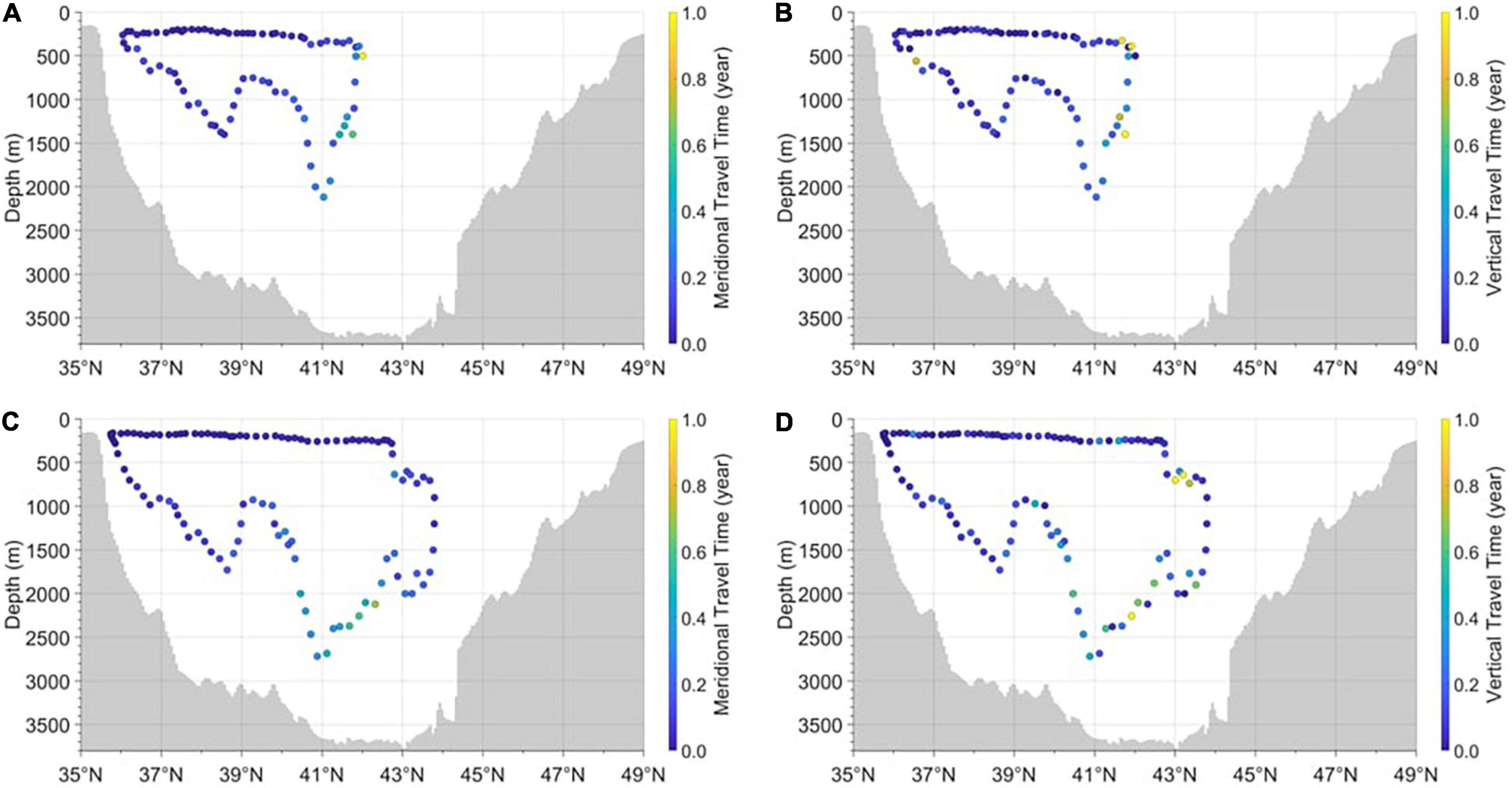
Figure 7. Meridional and vertical travel times of 0.3 Sv (A,B) and 0.13 Sv (C,D) streamlines for the deep convection case in the meridional overturning stream function. Turnover times of the 0.3 Sv (A,B) and 0.13 Sv (C,D) streamlines are 26.41 years (= 11.79 + 14.62) and 37.28 years (= 13.28 + 24.00), respectively.

FIGURE 8

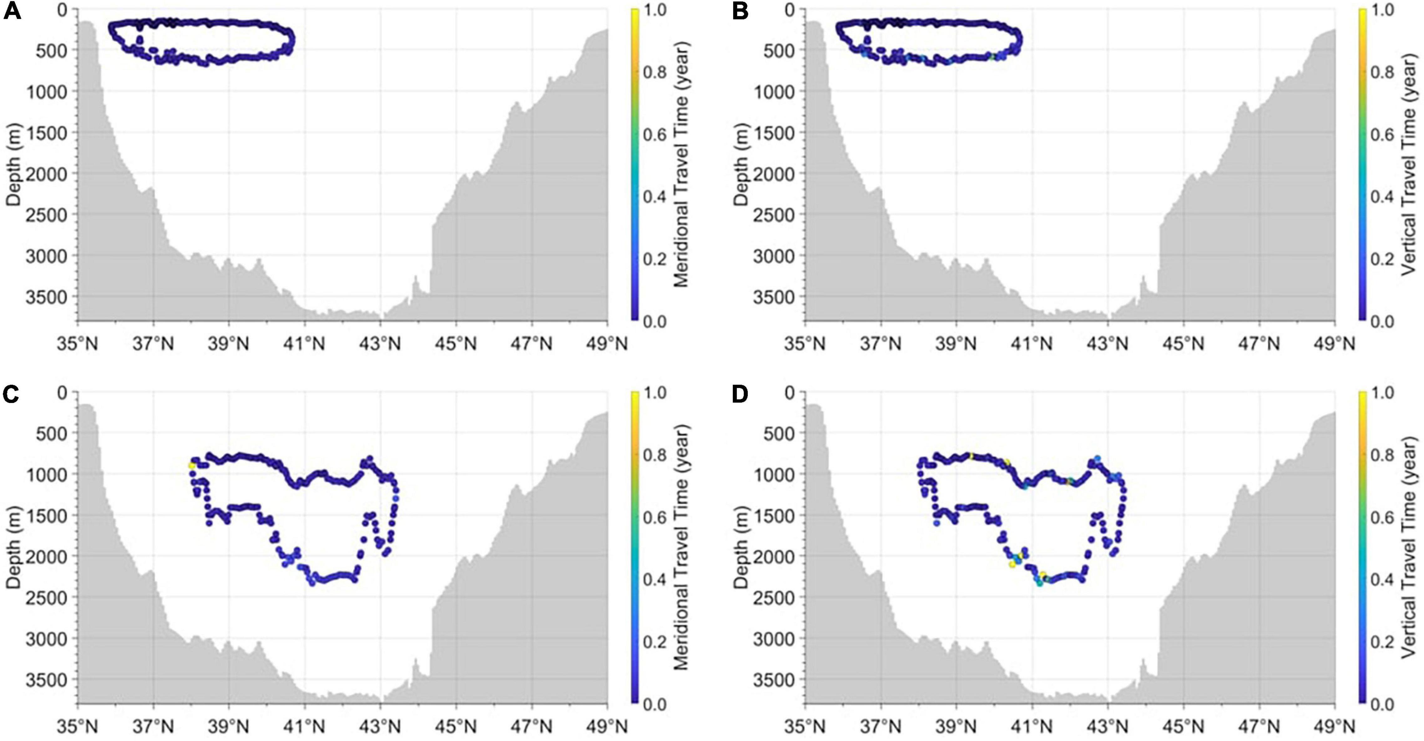
Figure 8. Meridional and vertical travel times of 0.2 Sv (A,B) and −0.3 Sv (C,D) streamlines for the shallow convection case in the meridional overturning stream function. Turnover times of the 0.2 Sv (A,B) and −0.3 Sv (C,D) streamlines are 8.68 years (= 2.22 + 6.46) and 36.76 years (= 9.98 + 26.78), respectively.

FIGURE 9

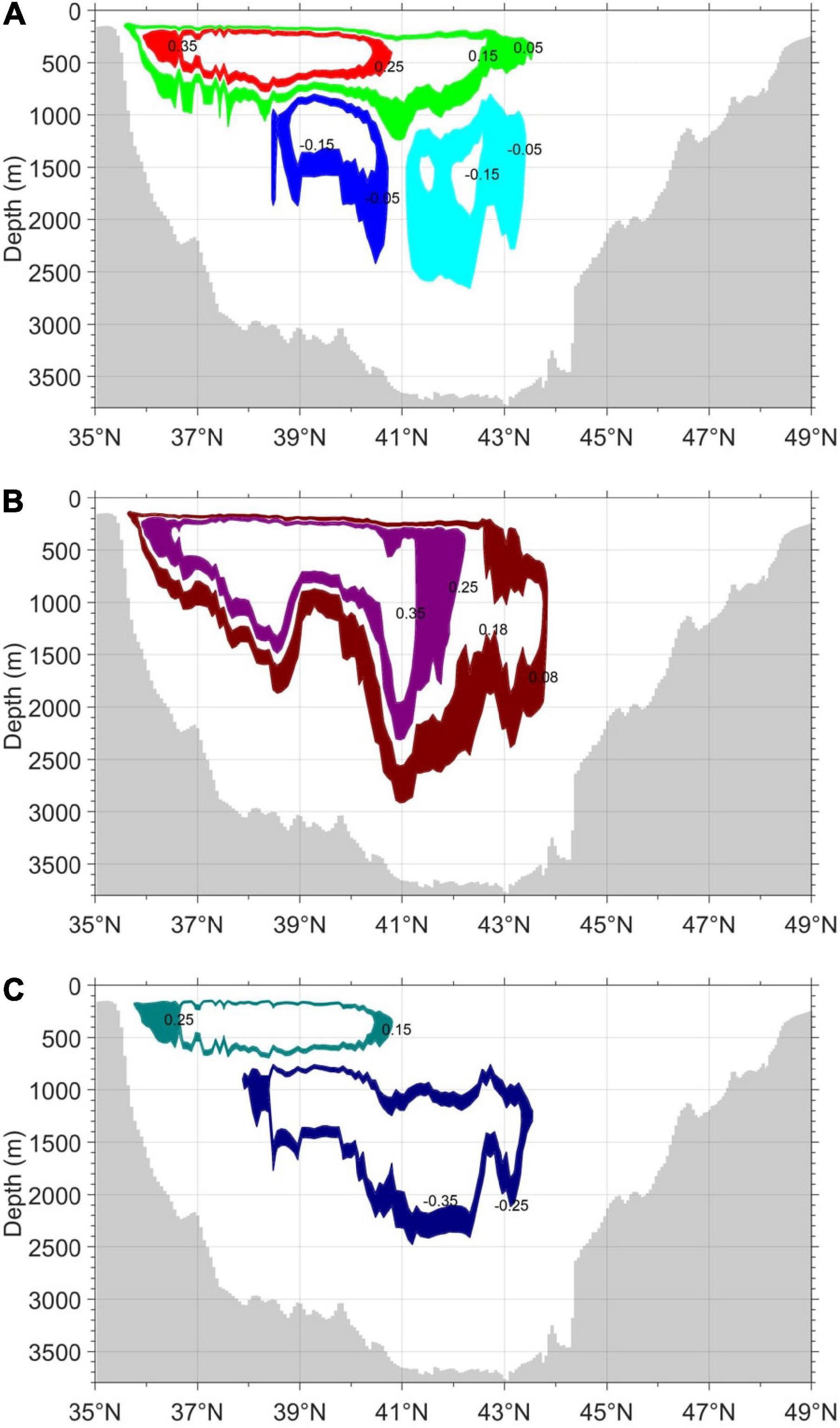
Figure 9. Turnover time (tot_v) in the (A) mean convection, (B) deep convection, and (C) shallow convection cases in the meridional overturning stream functions. The turnover times are 20.6 years (0.25–0.35 Sv streamlines, red), 34.5 years (0.05–0.15 Sv streamlines, green), 31.9 years (−0.15 to −0.05 Sv streamlines, blue), and 49.2 years (−0.15 to −0.05 Sv streamlines, cyan) years in the panel (A) mean convection case; 63.7 years (0.25–0.35 Sv streamlines, purple) and 79.8 years (0.08∼0.18 Sv streamlines, maroon) in the panel (B) deep convection case; and 13.3 years (0.15–0.25 Sv streamlines, teal) and 44.0 years (−0.25 to −0.35 Sv streamlines, navy) in the panel (C) shallow convection case, respectively.

However, it is difficult to directly measure the turnover time of the ES MOC because of slow vertical motions in the water column. Instead, approaches to indirectly estimate the turnover time scale based on chemical tracers have been commonly applied (Gamo and Horibe, 1983; Harada and Tsunogai, 1986; Watanabe et al., 1991; Tsunogai et al., 1993; Chen et al., 1995; Kumamoto et al., 1998). In these indirect methods, the concentration of tracers that have radioactive decay is measured to calculate the turnover times using simple models, considering the concentration difference between the water masses. For example, Watanabe et al. (1991) used a three-box model established by Harada and Tsunogai (1986), in which the exchange time of tracers can be calculated between the three water masses of cold surface water, warm surface water, and deep water to provide a turnover time of ∼100 years. In this model, tritium, which has a half-life of 12.4 years, was used as the tracer, eliminating the need to consider the exchange of CO2 at the air-sea interface. Kumamoto et al. (1998) observed an increase in ¹⁴C at the bottom of the ES, which indicated a rapid turnover of the bottom water. Using an equation based on the measurement of ¹⁴C at the surface and bottom waters, the turnover time was estimated to be ∼100 years, which was similar to that reported by Watanabe et al. (1991).

Approaches based on various tracers have advantages in diagnosing the conveyer-belt system in the ES by detecting the bias from the previous observations or by comparing it with the systems observed in other regions (Kim et al., 2001). However, the indirect calculation of the turnover time through comparison of tracer concentrations between water masses may lead to an inaccurate estimation or limited approximation of such a time scale. In addition, such indirect estimations do not consider the paths of the ES MOC, although the dynamics of tracer transport are crucial. Another method used to estimate the turnover time of the ES MOC considering its path is the numerical model. Kawamura et al. (2007) employed Geophysical Fluid Dynamics Laboratory (GFDL) Modular Ocean Model (MOM) to calculate the annual formation rate and turnover time of two water masses in the ES. Specifically, they applied a particle tracking method based on the Euler-Lagrangian technique (Awaji et al., 1991; Yoshikawa et al., 1999) to calculate the movement of water particles and their trajectories. However, the turnover time was calculated only for the two representative intermediate water masses, but not for the whole ES MOC, providing relatively short turnover time scales (∼22 and ∼2 years) for each water mass. An alternative method to estimate the MOC turnover time is to use the water volume divided by the water volume transport between two streamlines in an idealized ocean and the global ocean (Döös et al., 2012; Zika et al., 2012; Thompson et al., 2014). Moreover, these studies calculated the turnover time for different stream layers as a function of temperature and salinity.

In this study, we also applied numerical model data to address the turnover time of the ES MOC and its temporal changes, with emphasis on decadal change. We employed the HYbrid Coordinate Ocean Model (HYCOM) global reanalysis products with finer horizontal (0.08°) and vertical (32 layers) resolutions than those in the MOM simulation used by Kawamura et al. (2007) and in the nucleus for European modelling of the ocean (NEMO) employed by Döös et al. (2012). The HYCOM reanalysis product is well validated in comparison with the in situ observations of the ES (Hong et al., 2016; Han et al., 2020). In addition, the stream function approach is beneficial in calculating the turnover time because it provides both the pathways on which the water particles or masses move and the velocity at the corresponding positions, which can be calculated using the velocities and corresponding distances along the streamlines. According to the HYCOM reanalysis data, the ES MOC pattern was not consistent but showed temporal (decadal) changes. To calculate the stream functions, we averaged the flows for different periods considering these changes in the ES MOC, resulting in three different cases of ES MOC cells. We then estimated the turnover times for each case based on the different stream functions. Specifically, we considered different scenarios of water particle movement, even under the same case, by assuming that the particles could be exchanged between different cells. The resulting turnover times were then extended if the particles that moved to the adjacent convection cell returned to the original cell to complete the journey along the cells. Therefore, we could consider a dozen different scenarios that were possible for the estimation of turnover times.

However, before applying the model data, it was necessary to define the turnover time because there are different definitions for turnover time or similar time concepts. Several researchers define the residence time as the time taken for each material element to reach the outlet (Zimmerman, 1976; Shen and Haas, 2004), so it is defined at a particular location in the estuary, bay, or sea. Other researchers incorporate the possibility of the water parcel can reenter the estuary or sea; thus, the time stops as soon as the water parcel escapes from the boundaries of the estuary or sea in the case of “residence time” (Bolin and Rodhe, 1973; Takeoka, 1984; Delhez and Deleersnijder, 2006), and the time restarts immediately as the water parcel reenters the domain in the case of “exposure time” (Monsen et al., 2002; Delhez et al., 2004; de Brauwere et al., 2011). Other scientists used influence time as the rate of renewal of the original water by new water (Cucco and Umgiesser, 2006), which is related to the time required for outside particles to arrive at the observation point in the estuary or sea (Delhez et al., 2014). Moreover, the turnover time is defined by researchers as the time required for the concentration in the area of interest to decrease to e-folding (1/e) if the initial concentration is one (Prandle, 1984; Shen and Haas, 2004), and the local turnover time is computed for each segment or grid according to the mass reduction to e-folding in that segment or grid (Shen and Haas, 2004). The freshwater residence time is defined as the mean required time for freshwater to reside in the estuary prior to exiting, and the estuary residence time is the mean required time for a water parcel to remain in the estuary before exiting it (Barrera et al., 2001). Transit time is the time required for a passive particle to cross the estuary from the upstream region, and flushing time is the time needed for particles released throughout the estuary to exit the estuary (Lemagie and Lerczak, 2015).

The turnover time in this study was also distinguished from the turnover time in the study by Watanabe et al. (1991), with the turnover time referring to the simple vertical mixing time scale of the deep water, and the turnover time resulted in ∼100 years by incorporating the impact of cold surface water. As previously described, Kawamura et al. (2007) numerically calculated the turnover time as the amount of time that water particles circulated in the corresponding water mass prior to exiting. In this study, we calculated the turnover time by integrating the time required for the water particle to move between two sequential points on a streamline over the meridional plane, which provides the time for the water parcel to circulate along the streamline of the ES MOC. Overall, this study aimed to compare the turnover time scale estimated from highly accurate model data with turnover time estimations from previous studies using various radioactive tracers. Moreover, we investigated the possible range of the estimated time scale considering the temporal changes in the ES MOC. The remainder of this paper is organized as follows. The data and methods are described in the section “Data and Methods,” and the results and discussion are presented in the sections “Results” and “Discussion,” respectively. The summary and conclusion are presented in the section “Summary and Conclusion.”

Data and Methods

Data Sources

The HYbrid Coordinate Ocean Model (HYCOM) of the Global Ocean Forecasting System 3.0 (GOFS 3.0) and Global Reanalysis product (GLBb0.08), with Navy Coupled Ocean Data Assimilation (NCODA), has a horizontal resolution of 0.08° and employs a hybrid coordinate in which three vertical coordinates, namely isobars (pressure), isopycnals (density), and sigma levels (terrain), are used simultaneously. In this study, this reanalysis was used for the 20-year study period, from 1993 to 2012. The HYCOM data were then validated with the observed temperature, salinity, and velocity in the ES (Hong et al., 2016; Han et al., 2020).

Methods

The meridional overturning stream function (Ψ) was estimated by zonal and vertical integration of the meridional velocity (1 Sv = 10⁶m³s⁻¹) (Cunningham and Marsh, 2010; Kamenkovich and Radko, 2011; Han et al., 2013, 2020) as follows:

$$\mathrm{\Psi }(y,z,t)={\int }_{z_{bot}\left(y\right)}^z{\int }_{x_e(y,z^{{}^{\prime }})}^{x_w(y,z^{{}^{\prime }})}v(x,y,z^{\prime },t)\mathit{d}x\mathit{d}{z}^{\prime }(1)$$

Here, the meridional current v at longitude x, latitude y, depth z, and time t was integrated from the zonal easternmost point x_e to the westernmost point x_w, and from the bottom (z_bot) to the corresponding depth (z).

The turnover time following a streamline (tot_s) was calculated using the length (L_s) of the selected zonally integrated streamline (S) divided by the averaged velocity (${\overline{v}}_s$) following the streamline (S) as follows,

$$to{t}_s=\frac{L_s}{{\overline{v}}_s}={\sum }_{i=1}^n\frac{\left|y_{i+1}-y_i\right|}{\frac{v_{i+1}+v_i}{2}}+{\sum }_{i=1}^n\frac{\left|z_{i+1}-z_i\right|}{\frac{w_{i+1}+w_i}{2}}(2)$$

where y and z are the meridional and vertical locations, and v and w are the meridional and vertical velocities, respectively. We then selected smoothed streamlines and calculated the turnover time to exclude the travel time of stagnant water.

Results

Stream Function

In this study, we considered three cases of the ES MOC estimated from the stream function analysis based on the HYCOM data (Figure 2). The first case was obtained by averaging the HYCOM GOFS 3.0 reanalysis data for the 20-year study period, from 1993 to 2012 (Figures 2A, 3). This case was categorized as the “mean convection” case. In this case, four cells (cells ①, ②, ③, and ④) were obtained as shown in Figure 3A, by assuming that the shallow and deep convections were initiated around North Hamgyong Province in North Korea (East Sea Intermediate Water at approximately 41°N) and around Vladivostok (East Sea Central, Deep, and Bottom Waters at approximately 43°N), respectively. Therefore, the streamlines were selected at 41 (cell ①) and 43°N (cell ②) in accordance with Han et al. (2020). The contour lines (streamlines) of 0.3 and 0.1 Sv showed shallow cell pathways (cells ① and ② in Figure 3A), and those of −0.1 Sv showed deep cell pathways (cells ③ and ④ in Figure 3A).

During the 20-year reanalysis data period, the pattern of the cells could be divided into second (Figure 2B) and third (Figure 2C) cases considering the similarity of the convection pattern. In the second case, one large cell was formed and circulated the upper water directly into the deep region (Figures 2B, 4). Because we assumed that the water in this case started at Vladivostok (approximately 43°N) and there were same patterns for several years, the cell data of 8 years (1993, 2002, 2004–2009) out of the total 20-year data were averaged. The second case was categorized as a “deep convection” case. Contour lines (streamlines) of 0.3 and 0.13 Sv were selected to show the inner and outer pathways that form the one-cell convection and to display the deep convection around Vladivostok (cells ① and ② in Figure 4). The surface water sinks at a latitude of approximately 43°N to a depth of ∼3,000 m, and returns to the surface at a latitude of approximately 36°N after flowing southward along the lower part of the cell at depths of 1,000–2,000 m. The third case of the ES MOC stream functions consisted of a shallow cell above a 700-m depth, averaged in the years from 1996 to 2001 and from 2010 to 2012, as shown in Figures 2C, 5. Because we assumed that the water in this case originated from around North Hamgyong Province at approximately 41°N and there were similar patterns of reanalysis data for 9 years, the third case was categorized as a “shallow convection” case. In this case, two cells in shallow (<∼700 m) and deep (<∼2,500 m) waters were observed (cells ① and ② in Figure 5). The cell in the shallow water was confined to the southern part of the ES (36°N–41°N), whereas the pathway of the cell in the deep water occurred in the northern part (38°N–43.5°N). The three ES MOC cases with different cell numbers are summarized in Table 1. It should be noted that the cells in the three cases ranged over water depths from 300 to 3,000 m. Therefore, the flows in the surface area (<300 m) and deep area (>3,000 m) were not considered in this study.

TABLE 1

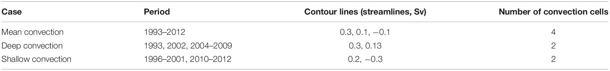
Table 1. Cells characteristics in the three ES MOC cases.

Turnover Time

Based on the three ES MOC cell cases listed in Table 1, the tot_s could be calculated following the different scenarios of water particle movement. These scenarios were based on assumptions that consider the possibility of water particle exchange between cells. For example, in mean convection, the turnover times could be obtained by integrating the circulation times of the three individual cells (cells ②, ③, and ④ in Figure 3A). In addition, we considered the possibility that the water particles in one cell could be transferred to another cell and move along the cell pathway. Based on this exchange possibility among the cells, we constructed three additional scenarios for the turnover times in the mean case, providing a total of seven scenarios to estimate tot_ss based on the ES MOC mean convection case (Tables 1, 2). For example, because the 0.3 Sv cell (cell ① marked with a solid line in Figures 3A,B) is confined within the 0.1 Sv cell (cell ② marked with a dashed line in Figures 3A,B), the water particle in the 0.3 Sv cell (cell ①) could not be directly transported to the −0.1 Sv cells (left cell ③ marked with dot-dashed line and right cell ④ marked with dot-dot-dashed line in Figures 3A,C), crossing the 0.1 Sv cell (the cell ②) (scenario 1 in Table 2). Therefore, the water particles could only be exchanged between cells ② and ③, and between cells ② and ④. Therefore, a turnover time scenario could be determined by considering that a water particle in cell ② moved to cell ③ and then back to cell ② after circulating cell ③ to complete its journey in the ES MOC (scenario 5 in Table 2). Similarly, another scenario could be constructed by considering the possibility that a water particle in cell ② was transferred to cell ④ and returned to cell ② so that the turnover time of the particle could be estimated by adding the circulation times for cells ② and ④ (scenario 6 in Table 2). In addition, as shown in Figure 3C, a water particle in cell ② could be moved to cell ④. After circulating cell ④ in the anti-clockwise direction, however, the particle could also be transferred to cell ③ instead of returning to cell ②. Finally, this water particle could then join back to cell ② after circulating cell ③. Therefore, the final turnover time could be calculated by adding the circulation times of cells ②, ③, and ④, resulting in a longest turnover time compared to the other scenarios in which the water particles circulated each cell only once or circulate over two adjacent cells (scenario 7 in Table 2).

TABLE 2

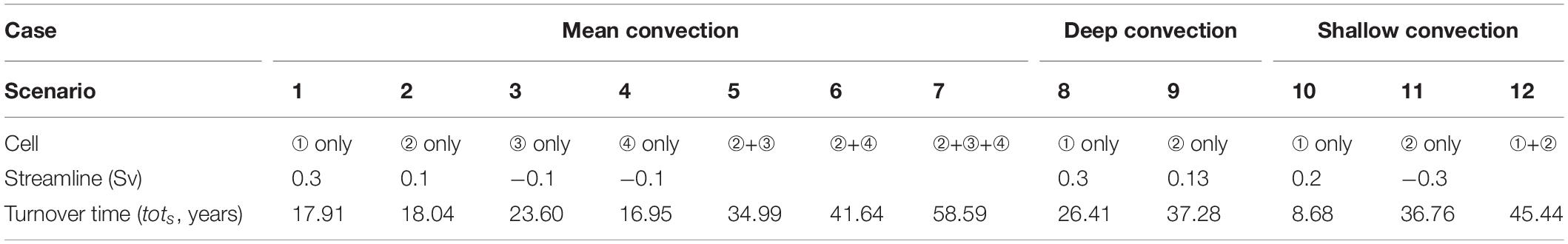
Table 2. Turnover time (tot_s) scenarios for the mean, deep, and shallow convection cases in the ES MOC.

The tot_ss calculated for the seven scenarios in the mean convection case were as follows: cells ① and ② ranged from ∼300 to ∼700 m, and from ∼300 to ∼900 m depths, respectively, as shown in Figure 3B. Moreover, the turnover times of these cells were 17.91 years (cell ①, scenario 1 in Table 2) and 18.04 years (cell ②, scenario 2 in Table 2), respectively. The water depths of cells ②, ③, and ④ for the mean convection case ranged from ∼300 m to ∼2,500 m (scenario 7 in Table 2) as shown in Figure 3C. The turnover times of these cells were 34.99 years (cells ②+③, scenario 5 in Table 2), 41.64 years (cells ②+④, scenario 6 in Table 2), and 58.59 years (cells ②+③+④, scenario 7 in Table 2). The results of tot_ss for the seven scenarios for the mean convection case are listed in Table 2.

The meridional and vertical turnover times were calculated separately to investigate the turnover time. Figure 6 shows the method for calculating the turnover time of each cell meridionally and vertically, and the dots in the figure represent the locations where the travel time was calculated in the meridional and vertical directions. The colors of the dots denote the travel time between two adjacent locations in each direction, as calculated using Eq. 2. The left four panels in Figure 6 show the travel time between the two adjacent dots in the meridional direction for the four convection streamlines shown in Figure 3A, whereas the right four panels show the travel time in the vertical direction for the corresponding convection streamlines. The meridional travel times were long (yellow color) in the north in Figures 6A,C, and deep in Figures 6E,G. Moreover, the vertical travel times were longer (yellow color) at several locations (Figures 6B,D,F,H). The tot_s of each cell could be calculated by the summation of the travel times in the meridional and vertical directions. For example, in the case of cell ①, the tot_s was obtained by adding the travel time in the meridional direction (3.62 years, as shown in Figure 6A) to the travel time in the vertical direction (14.29 years, as shown in Figure 6B), equaling a tot_s of 17.91 years for the cell ①. Similarly, the tot_s for convection cells ②, ③, and ④ could be calculated by adding the travel times in both directions, as shown in Figures 6C–H. The long travel times between the two locations were typically observed in the deep northern waters, but this trend was not always observed in the deep and shallow convection cases in Figures 7, 8.

The estimation of turnover times for the deep convection case (Table 1) was simpler because the ES MOC consists of only one large meridional circulation. As shown in Figures 2B, 4 the two streamlines estimated over 0.3 Sv (cell ① in Figure 4) and 0.13 Sv (cell ② in Figure 4) formed two closed loops of the cells. The turnover times for the cells were 26.41 years for cell ① and 37.28 years for cell ②. The results are summarized in scenarios 8 and 9 of Table 2. The method of calculating tot_ss for cells ① and ② in Figure 4 was the same as that for the mean convection case, with the travel times in the meridional and vertical directions added to provide the total turnover time for each cell (Figure 7). A similar approach could be applied to the shallow convection case, as shown in Figures 2C, 5. The turnover times could be estimated individually for the two cells by adding the travel times in the meridional and vertical directions (Figure 8). In addition, other tot_ss could be calculated by summing the tot_ss of cells ① and ②, considering that the water particle was exchanged between the cells and assuming that the particles that circulate cell ② would join back to cell ① to complete its journey over the ES MOC in Figure 5. The resulting tot_ss for the shallow convection case were 8.68 years for cell ①, 36.76 years for cell ②, and 45.44 years for cells ①+② (scenarios 10, 11, and 12 of Table 2).

Discussion

The results of this study indicated several possible scenarios for the ES MOC pathways and resultant turnover times. These findings were based on a new approach using modeled data, which was distinguished from the turnover times based on traditional chemical tracer estimations. In this approach, which calculates the stream functions in the 2-D meridional plane, realistic passages of water particles could be visualized by identifying the locations of vertical movement (where the water rises and sinks), and the horizontal movement (where the water flows southward and northward). In addition, the water particle pathways could be modified by considering the water particle exchange between two adjacent cells, providing various water particle pathway scenarios. The turnover times depended on the pathways and cells, and they ranged from 8.68 to 58.59 years. The turnover times calculated in this study (maximum ∼59 years) were less than those calculated from chemical tracers, such as CFC, ¹⁴C, tritium, and ²²⁶Ra (∼100 years) (Harada and Tsunogai, 1986; Watanabe et al., 1991; Tsunogai et al., 1993; Chen et al., 1995; Kumamoto et al., 1998). The reason for this difference remains unclear. However, we calculated the turnover times by selecting streamlines that sunk at approximately 41°N and 43°N, and assumed that the water particles followed these streamlines. Water particles could not rise above a depth of 300 m, nor sink below a depth of 3,000 m in this study. It is because the surface currents above the 300 m depth do not make a closed ES MOC path, which is owing to the Korea/Tsushima, Tsugaru, Soya, and Tatarsky Straits. Also, it is because the stream function data were not enough below the 3,000 m depth owing to the scarceness of velocity data at such depths. These likely resulted in an underestimation of the calculated turnover time in this study.

Another possible reason for the discrepancy in our results could be our assumption that the water particles were exchanged only once during their journey along the ES MOC. However, it is also possible that the water particles transferred to the cell in the deep water remained within the cell for two cycles before finally joining the cell in the shallow water. In that case the total turnover time would increase and, in reality, there could be many different exchange combinations to provide a wide range of turnover time scales. For example, in the three-cell (Figure 3C) mean convection case, the turnover times could be extended if the water particle that started in cell ② moved to cell ④ and cell ③, then remained at cell ③ for two cycles, giving a turnover time of 105.79 years (cells ②+④+③+③+③). However, this extended turnover time would not be considered as an official result because matching the time scale with those in previous studies was not the purpose of this study.

Compared to the turnover times calculated based on the stream function (tot_s) in this study, another definition of turnover time based on the water volume (tot_v) was suggested, calculated by dividing the water volume (△V) by the water volume transport (△Ψ) between the corresponding two streamlines (Döös et al., 2012; Zika et al., 2012; Thompson et al., 2014), as follows

$$to{t}_v=\frac{\mathrm{△}V}{\mathrm{△}\mathrm{\Psi }}(3)$$

The tot_v was then estimated for the three cases listed in Table 1 for a comparison with tot_s; we selected two adjacent streamlines according to those of tot_s in the previous section. For example, two adjacent 0.25 Sv and 0.35 Sv streamlines of tot_v (red in Figure 9) were selected according to ± 0.05 Sv of the 0.3 Sv streamline of tot_s (Figure 2A). In Figures 9A–C, the stream functions at different levels were contoured for the corresponding three cases, with different colors marking the size of the water volume between the two adjacent streamlines. For example, the water volume between the 0.25 Sv and 0.35 Sv streamlines in the mean convection case was ∼6.5 × 10¹³ m³, and the water volume transport between the 0.25 Sv and 0.35 Sv streamlines was 0.1 × 10⁶ m³ s^–1 (red color), as shown in Figure 9A. Therefore, according to Eq. 3, the tot_v between the 0.25 Sv and 0.35 Sv streamlines was 6.5 × 10¹³ (m³)/0.1 × 10⁶ (m³ s^–1) ≈ 6.5 × 10⁸ (sec) ≈ 20.6 (years). This tot_v was longer than that calculated for the 0.3 Sv streamline (tot_s, ∼17.9 years) because the tot_v assumed that the water mass between the 0.25 Sv and 0.35 Sv streamlines flowed approximately along the original 0.3 Sv streamline and that its pathway was larger than that of the smoothed 0.3 Sv streamline. Similarly, the other tot_vs for the mean convection case were 34.5 years (between the 0.05 Sv and 0.15 Sv streamlines; green), 31.9 years (between the −0.15 Sv and −0.05 Sv streamlines; blue; south), and 49.2 years (between the −0.15 Sv and −0.05 Sv streamlines; cyan; north) (Figure 9A and Table 3). We selected these streamlines to compare the tot_v and tot_s. The tot_vs for the deep convection case were 63.7 years (between the 0.25 Sv and 0.35 Sv streamlines; purple) and 79.8 years (between the 0.08 Sv and 0.18 Sv streamlines; maroon) (Figure 9B and Table 3). The tot_vs in the shallow convection case were 13.3 years (between the 0.15 Sv and 0.25 Sv streamlines; teal) and 44.0 years (between the −0.35 Sv and −0.25 Sv streamlines; navy) (Figure 9C and Table 3). These tot_vs were longer than tot_ss because the latter was calculated along smoothed streamlines (Figures 6–8) and the former was calculated by dividing the volume by the volume transport between the two original and unsmoothed streamlines (Figure 9). It was noted that the longest tot_s based on Eq. 2 was 58.59 years when the water particle circulated the three cells (mean convection case, scenario 7), as shown in Table 2. However, the longest tot_v based on Eq. 3 was 79.8 years for the deep convection case as shown in Table 3. This is because tot_s increased when the water particle moving along the streamline traveled over a larger number of cells because of the exchange between the cells (i.e., tot_s was the longest when the water particle traveled over the largest [three] number of cells in Figure 3C). Conversely, tot_v increased when the water volume (per water volume transport, 0.1 Sv in this study) increased, as indicated by Eq. 3, resulting in the longest turnover time when the water volume was the largest in the deep convection case (maroon color in Figure 9B). It is also interesting to note that the longest tot_v of 79.8 years was close to the estimation of ∼100 years based on chemical tracers, probably because of the similar mechanisms of turnover time estimation.

TABLE 3

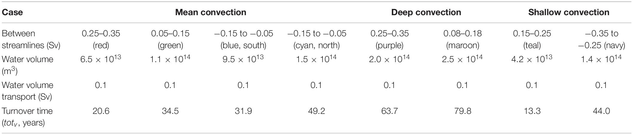
Table 3. Turnover time (tot_v) for the mean, deep, and shallow convection cases in the ES MOC.

The chemical tracing turnover times of the ES bottom water, around 100 years (e.g., Gamo and Horibe, 1983; Kumamoto et al., 1998), were calculated by assuming that the bottom water (below a depth of 2,000 m) was exchanged with the deep water (above a depth of 2,000 m). However, our calculation in this study was estimated based on the circulation along the streamline (Eq. 2), and water volume transport between streamlines (Eq. 3). This suggests that biogeochemists can observe the tracers and calculate the turnover time in a new way. We could calculate the turnover time of the water below 2,000 m depth (tot_2,000m) using the water volume below 2,000 m depth in the ES (△V_2,000m, 0.4 × 10¹⁵ m³) divided by the water volume transports at a 2,000 m depth in mean, deep, and shallow convection cases (△Ψ, −0.10 Sv, 0.30 Sv, and −0.30 Sv in Figure 2 and Table 1) as follows, and the results were ∼125.5, ∼41.8, and ∼41.8 years.

$$to{t}_{2,000m}=\frac{\mathrm{△}{V}_{2,000m}}{\mathrm{△}{\mathrm{\Psi }}_{2,000m}}(4)$$

The water which sinks and reaches a depth of around 700 m always flows southward, while the water below a depth of 2,000 m flows southward in deep convection case (for 8 years such as 1993, 2002, 2004–2009) and northward in shallow convection case (for 9 years from 1996 to 2001 and from 2010 to 2012) in Figures 2–5. This reversal of the water flow direction below the 2,000 m depth between the deep and shallow convection cases explained why the turnover time (tot_2,000m) in the mean convection case is longer than those in the deep and shallow convection cases. Also, we suggested the pathways of the ES MOC in this study, which were related to the topography in the ES. Marine biogeochemists can measure the biogeochemical tracers or matters along the pathways of the ES MOC, and they can deduce the origin of those materials. Thus, research plans can be established that refer to the pathways of the turnover time in this study. This physical turnover time calculation and its biogeochemical utilization can be applied to areas adjacent to the ES such as Yellow Sea and East China Sea, and other regional seas and open oceans.

Moreover, we used the results of the global simulation with the data assimilation to calculate the turnover time, and applied the stream function approach to determine the pathways and turnover times for the various ES MOC cases. However, there is a drawback associated with the stream function approach: stream functions are obtained only in the 2-D meridional plane. Therefore, the longitudinal flow motions and 3-D circulations could not be considered as currents that move to the west or east in the middle of the ES (e.g., Figure 18 of Yun et al., 2004; Figure 4 of Park et al., 2010). The 2-D consideration of the ES MOC using stream functions could therefore lead to an underestimation of its time scale. Other approaches such as particle tracking or dye experiments with numerical simulations longer than 20 years could be explored in future studies to estimate the turnover time in the ES and to evaluate the accuracy of the approach used in this study.

Summary and Conclusion

In this study, the turnover times of the ES MOC were estimated using a global HYCOM reanalysis with data assimilation for 20-year period (1993–2012). This method is distinguished from the traditional methods in which the turnover times in the ES were estimated indirectly using chemical tracers and directly using the numerical simulation of water particles of the intermediate water, not deep water. Specifically, this method is advantageous because the pathways of water particle movement can be identified by integrating the motions along streamlines, which also provides the possible passages of tracers.

Three cases based on the integration of travel time were selected for the ES MOC. The first case was a “mean convection case” obtained by averaging all the data over a 20-year period, from 1993 to 2012. The second and third cases were obtained by averaging the reanalysis data for selected years with similar patterns: 1993, 2002, and 2004–2009 for the second ES MOC case (deep convection case), and 1996–2001 and 2010–2012 for the third case (shallow convection case). As a result, the ES MOC pattern was different between the cases as four meridional overturning cells were obtained in the first case, and only one cell was determined for the second case. In the third case, two cells, the upper and lower cells, were observed. The turnover times were then calculated by integrating the travel times of the water particles along the streamlines between two locations. A variety of pathways and turnover times in the ES MOC could be estimated considering that the water particles were exchanged between adjacent cells. Therefore, several overturning pathways were obtained for each ES MOC case by assuming different exchange scenarios.

The shortest turnover time of 8.68 years was obtained in the scenario where the water particles circulated through the upper cell only, without exchange with the lower cell in the third ES MOC case (shallow convection case, scenario 10 in Table 2). Conversely, the longest turnover time was 58.59 years, which was obtained from the first ES MOC case (mean convection case) by considering the water particle exchange between all three cells – that is, the water particle that left the upper cell also circulated the two lower cells until finally returning to the original location in the upper cell to complete the journey along the ES MOC (scenario 7 in Table 2). This turnover time was approximately half of that estimated by chemical tracers in previous studies (Watanabe et al., 1991; Kumamoto et al., 1998); however it was longer than that estimated using a numerical approach (Kawamura et al., 2007). The reason for this discrepancy is not clear. However, the HYCOM reanalysis data used in this study was validated and assimilated using various global ocean measurements, providing useful information for various studies. In addition, the turnover times in this study can be extended by employing additional water particle exchange scenarios. For example, the turnover time could reach ∼100 years if we considered that the water particles circulated the deep cell multiple times before returning to the shallow cell, which was excluded in this study because matching the turnover time scale with previous studies was not the purpose of this study. The method in this study can also be applied to estimate the turnover times in the global ocean and in other basins, which would aid in forecasting global and regional overturning circulations in a warming climate.

Data Availability Statement

The original contributions presented in the study are included in the article/supplementary material, further inquiries can be directed to the corresponding author.

Author Contributions

MH performed all data analysis. MH and YC contributed to the writing the manuscript. D-JK originally gave us an idea of this study. MH, YC, H-WK, D-JK, and YK contributed to the conceptualization and interpretation of the results. All authors contributed to the article and approved the submitted version.

Funding

This research was a part of the projects entitled “Establishment of the ocean research station in the jurisdiction zone and convergence research” and “Study on air-sea interaction and process of rapidly intensifying typhoon in the northwestern Pacific” funded by the Ministry of Oceans and Fisheries, and also supported by the National Research Foundation of Korea grant funded by the Korea government (NRF-2020R1F1A1070398). This research was partially supported by “Biogeochemical cycling and marine environmental change studies” (PE99912) and “Influences of the Northwest Pacific circulation and climate variability on the Korean water changes and material cycle I - The role of Jeju warm current and its variability” (PE99911).

Conflict of Interest

The authors declare that the research was conducted in the absence of any commercial or financial relationships that could be construed as a potential conflict of interest.

Publisher’s Note

All claims expressed in this article are solely those of the authors and do not necessarily represent those of their affiliated organizations, or those of the publisher, the editors and the reviewers. Any product that may be evaluated in this article, or claim that may be made by its manufacturer, is not guaranteed or endorsed by the publisher.

References

Awaji, T., Akitomo, K., and Imasato, N. (1991). Numerical study of shelf water motion driven by the Kuroshio: Barotropic model. J. Phys. Oceanogr. 21, 11–27. doi: 10.1175/1520-04851991021<0011:NSOSWM<2.0.CO;2

CrossRef Full Text | Google Scholar

Barrera, J., Cantilli, R., Davis, I., Dettmann, E. H., Fisher, J., Gardner, T., et al. (2001). Nutrient Criteria Technical Guidance Manual: Estuarine and Coastal Marine Waters. Washington, D.C: U.S. Environmental Protection Agency, Office of Water.

Google Scholar

Bolin, B., and Rodhe, H. (1973). A note on the concepts of age distribution and transit time in natural reservoirs. Tellus 25, 58–62. doi: 10.1111/j.2153-3490.1973.tb01594.x

CrossRef Full Text | Google Scholar

Chang, K.-I., Zhang, C.-I., Park, C., Kang, D.-J., Ju, S.-J., Lee, S.-H., et al. (2016). Oceanography of the East Sea (Japan Sea). Heidelberg: Springer.

Google Scholar

Chen, C. T. A., Wang, S. L., and Bychkov, A. S. (1995). Carbonate chemistry of the sea of Japan. J. Geophys. Res. 100, 13737–13745. doi: 10.1029/95JC00939

CrossRef Full Text | Google Scholar

Cho, Y.-K., and Kim, K. (1998). Structure of the Korea strait bottom cold water and its seasonal variation in 1991. Cont. Shelf Res. 18, 791–804. doi: 10.1016/S0278-4343(98)00013-2

CrossRef Full Text | Google Scholar

Cucco, A., and Umgiesser, G. (2006). Modeling the venice lagoon residence time. Ecol. Model. 193, 34–51. doi: 10.1016/j.ecolmodel.2005.07.043

CrossRef Full Text | Google Scholar

Cunningham, S. A., and Marsh, R. (2010). Observing and modeling changes in the Atlantic MOC. Wiley Interdiscip. Rev. Clim. Change 1, 180–191. doi: 10.1002/wcc.22

CrossRef Full Text | Google Scholar

de Brauwere, A., De Brye, B., Blaise, S., and Deleersnijder, E. (2011). Residence time, exposure time and connectivity in the Scheldt Estuary. J. Mar. Syst. 84, 85–95. doi: 10.1016/j.jmarsys.2010.10.001

CrossRef Full Text | Google Scholar

Delhez, É. J., De Brye, B., De Brauwere, A., and Deleersnijder, E. (2014). Residence time vs influence time. J. Mar. Syst. 132, 185–195. doi: 10.1016/j.jmarsys.2013.12.005

CrossRef Full Text | Google Scholar

Delhez, É. J., and Deleersnijder, É (2006). The boundary layer of the residence time field. Ocean Dyn. 56, 139–150. doi: 10.1007/s10236-006-0067-0

CrossRef Full Text | Google Scholar

Delhez, É. J., Heemink, W. A., and Deleersnijder, É. (2004). Residence time in a semi-enclosed domain from the solution of an adjoint problem. Estuar. Coast. Shelf Sci. 61, 691–702. doi: 10.1016/j.ecss.2004.07.013

CrossRef Full Text | Google Scholar

Döös, K., Nilsson, J., Nycander, J., Brodeau, L., and Ballarotta, M. (2012). The world ocean thermohaline circulation. J. Phys. Oceanogr. 42, 1445–1460. doi: 10.1175/JPO-D-11-0163.1

CrossRef Full Text | Google Scholar

Gamo, T., and Horibe, Y. (1983). Abyssal circulation in the Japan Sea. J. Oceanogr. 39, 220–230. doi: 10.1038/ncomms1156

PubMed Abstract | CrossRef Full Text | Google Scholar

Han, M., Cho, Y.-K., Kang, H.-W., and Nam, S. (2020). Decadal changes in meridional overturning circulation in the East Sea (Sea of Japan). J. Phys. Oceanogr. 50, 1773–1791. doi: 10.1175/JPO-D-19-0248

CrossRef Full Text | Google Scholar

Han, M., Kamenkovich, I., Radko, T., and Johns, W. E. (2013). Relationship between air–sea density flux and isopycnal meridional overturning circulation in a warming climate. J. Clim. 26, 2683–2699. doi: 10.1175/JCLI-D-11-00682.1

CrossRef Full Text | Google Scholar

Harada, K., and Tsunogai, S. (1986). 226Ra in the Japan Sea and the residence time of the Japan Sea water. Earth Planet. Sci. Lett. 77, 236–244. doi: 10.1016/0012-821X(86)90164-0

CrossRef Full Text | Google Scholar

Hong, J., Seo, S., Jeon, C., Park, J.-H., Park, Y.-G., and Min, H. S. (2016). Evaluation of temperature and salinity fields of HYCOM reanalysis data in the east sea. Ocean Polar Res. 38, 271–286. doi: 10.4217/OPR.2016.38.4.271

CrossRef Full Text | Google Scholar

Ichiye, T. (1984). “Some problems of circulation and hydrography of the Japan Sea and the Tsushima current,” in Ocean Hydrodynamics of the Japan and East China Seas. Elsevier Oceanography Series, ed. T. Ichiye (Amsterdam: Elsevier), 15–54. doi: 10.1016/s0422-9894(08)70289-7

CrossRef Full Text | Google Scholar

Kamenkovich, I., and Radko, T. (2011). Role of the Southern Ocean in setting the Atlantic stratification and meridional overturning circulation. J. Mar. Res. 69, 277–308. doi: 10.1357/002224011798765286

CrossRef Full Text | Google Scholar

Kawamura, H., Yoon, J.-H., and Ito, T. (2007). Formation rate of water masses in the Japan Sea. J. Oceanogr. 63, 243–253. doi: 10.1007/s10872-007-0025-6

CrossRef Full Text | Google Scholar

Kim, K., Kim, K. R., Min, D. H., Volkov, Y., Yoon, J. H., and Takematsu, M. (2001). Warming and structural changes in the East (Japan) Sea: a clue to future changes in global oceans? Geophys. Res. Lett. 28, 3293–3296. doi: 10.1029/2001GL013078

CrossRef Full Text | Google Scholar

Kim, K. R., Kim, G., Kim, K., Lobanov, V., Ponomarev, V., and Salyuk, A. (2002). A sudden bottom-water formation during the severe winter 2000–2001: the case of the East/Japan Sea. Geophys. Res. Lett 29, 75–71–75–74. doi: 10.1029/2001GL014498

CrossRef Full Text | Google Scholar

Kim, T.-H., and Kim, G. (2012). Important role of colloids in the cycling of 210Po and 210Pb in the ocean: results from the East/Japan Sea. Geochim. Cosmochim. Acta 95, 134–142. doi: 10.1016/j.gca.2012.07.029

CrossRef Full Text | Google Scholar

Kim, Y.-G., and Kim, K. (1999). Intermediate waters in the East/Japan Sea. J. Oceanogr. 55, 123–132. doi: 10.1023/A:1007877610531

CrossRef Full Text | Google Scholar

Kim, Y. H., Kim, Y. B., Kim, K., Chang, K. I., Lyu, S. J., Cho, Y. K., et al. (2006). Seasonal variation of the Korea strait bottom cold water and its relation to the bottom current. Geophys. Res. Lett. 33:6. doi: 10.1029/2006GL027625

CrossRef Full Text | Google Scholar

Kumamoto, Y. I., Yoneda, M., Shibata, Y., Kume, H., Tanaka, A., Uehiro, T., et al. (1998). Direct observation of the rapid turnover of the Japan Sea bottom water by means of AMS radiocarbon measurement. Geophys. Res. Lett. 25, 651–654. doi: 10.1029/98GL00359

CrossRef Full Text | Google Scholar

Lemagie, E. P., and Lerczak, J. A. (2015). A comparison of bulk estuarine turnover timescales to particle tracking timescales using a model of the Yaquina Bay Estuary. Estuaries Coast. 38, 1797–1814. doi: 10.1007/s12237-014-9915-1

CrossRef Full Text | Google Scholar

Min, H. S., and Kim, C.-H. (2006). Water mass formation variability in the intermediate layer of the East Sea. Ocean Sci. J. 41, 255–260. doi: 10.1007/BF03020629

CrossRef Full Text | Google Scholar

Monsen, N. E., Cloern, J. E., Lucas, L. V., and Monismith, S. G. (2002). A comment on the use of flushing time, residence time, and age as transport time scales. Limnol. Oceanogr. 47, 1545–1553. doi: 10.4319/lo.2002.47.5.1545

CrossRef Full Text | Google Scholar

Park, J., and Lim, B. (2018). A new perspective on origin of the East Sea Intermediate water: observations of Argo floats. Prog. Oceanogr. 160, 213–224. doi: 10.1016/j.pocean.2017.10.015

CrossRef Full Text | Google Scholar

Park, Y.-G., Choi, A., Kim, Y. H., Min, H. S., Hwang, J. H., and Choi, S.-H. (2010). Direct flows from the Ulleung Basin into the Yamato Basin in the East/Japan Sea. Deep Sea Res. 1 Oceanogr. Res. Pap. 57, 731–738. doi: 10.1016/j.dsr.2010.03.006

CrossRef Full Text | Google Scholar

Prandle, D. (1984). A modelling study of the mixing of 137Cs in the seas of the European continental shelf. Philos. Trans. R. Soc. Lond. A 310, 407–436. doi: 10.1098/rsta.1984.0002

CrossRef Full Text | Google Scholar

Shen, J., and Haas, L. (2004). Calculating age and residence time in the tidal York River using three-dimensional model experiments. Estuar. Coast. Shelf Sci. 61, 449–461. doi: 10.1016/j.ecss.2004.06.010

CrossRef Full Text | Google Scholar

Stouffer, R. J., Yin, J., Gregory, J., Dixon, K., Spelman, M., Hurlin, W., et al. (2006). Investigating the causes of the response of the thermohaline circulation to past and future climate changes. J. Clim. 19, 1365–1387. doi: 10.1175/JCLI3689.1

CrossRef Full Text | Google Scholar

Takeoka, H. (1984). Fundamental concepts of exchange and transport time scales in a coastal sea. Cont. Shelf Res. 3, 311–326. doi: 10.1016/0278-4343(84)90014-1

CrossRef Full Text | Google Scholar

Talley, L., Min, D., Lobanov, V., Luchin, V., Ponomarev, V., Salyuk, A., et al. (2006). Japan/East Sea water masses and their relation to the sea’s circulation. Oceanography 19, 32–49. doi: 10.1029/2002GL016451

CrossRef Full Text | Google Scholar

Talley, L. D., Lobanov, V., Ponomarev, V., Salyuk, A., Tishchenko, P., Zhabin, I., et al. (2003). Deep convection and brine rejection in the Japan Sea. Geophys. Res. Lett. 30:1159. doi: 10.5670/oceanog.2006.42

CrossRef Full Text | Google Scholar

Thompson, B., Nycander, J., Nilsson, J., Jakobsson, M., and Döös, K. (2014). Estimating ventilation time scales using overturning stream functions. Ocean Dyn. 64, 797–807. doi: 10.1007/s10236-014-0726-5

CrossRef Full Text | Google Scholar

Tsunogai, S., Watanabe, Y. W., Harada, K., Watanabe, S., Saito, S., and Nakajima, M. (1993). “Dynamics of the Japan Sea deep water studied with chemical and radiochemical tracers,” in Elsevier Oceanography Series, ed. T. Teramoto (Amsterdam: Elsevier), 105–119. doi: 10.1016/s0422-9894(08)71321-7

CrossRef Full Text | Google Scholar

Watanabe, Y., Watanabe, S., and Tsunogai, S. (1991). Tritium in the Japan Sea and the renewal time of the Japan Sea deep water. Mar. Chem. 34, 97–108. doi: 10.1016/0304-4203(91)90016-P

CrossRef Full Text | Google Scholar

Wunsch, C. (2002). What is the thermohaline circulation? Science 298, 1179–1181. doi: 10.1126/science.1079329

PubMed Abstract | CrossRef Full Text | Google Scholar

Yoon, S.-T., Chang, K.-I., Nam, S., Rho, T., Kang, D.-J., Lee, T., et al. (2018). Re-initiation of bottom water formation in the East Sea (Japan Sea) in a warming world. Sci. Rep. 8:1576. doi: 10.1038/s41598-018-19952-4

PubMed Abstract | CrossRef Full Text | Google Scholar

Yoshikawa, Y., Awaji, T., and Akitomo, K. (1999). Formation and circulation processes of intermediate water in the Japan Sea. J. Phys. Oceanogr. 29, 1701–1722. doi: 10.1175/1520-04851999029<1701:FACPOI<2.0.CO;2

CrossRef Full Text | Google Scholar

Yun, J.-Y., Magaard, L., Kim, K., Shin, C.-W., Kim, C., and Byun, S.-K. (2004). Spatial and temporal variability of the North Korean Cold Water leading to the near-bottom cold water intrusion in Korea Strait. Prog. Oceanogr. 60, 99–131. doi: 10.1016/j.pocean.2003.11.004

CrossRef Full Text | Google Scholar

Zika, J. D., England, M. H., and Sijp, W. P. (2012). The ocean circulation in thermohaline coordinates. J. Phys. Oceanogr. 42, 708–724. doi: 10.1175/JPO-D-11-0139.1

CrossRef Full Text | Google Scholar

Zimmerman, J. T. F. (1976). Mixing and flushing of tidal embayments in the western Dutch Wadden Sea part I: distribution of salinity and calculation of mixing time scales. Neth. J. Sea Res. 10, 149–191. doi: 10.1016/0077-7579(76)90013-2

CrossRef Full Text | Google Scholar