Characteristics of Ichthyoplankton Communities and Their Relationship With Environmental Factors Above the Ninety East Ridge, Eastern Indian Ocean

The Ninety East Ridge is a submarine north–south oriented volcanic ridge in the eastern Indian Ocean. Surface-layer ichthyoplankton collected in this area from September to October were identified by combined morphological and molecular (DNA barcoding) techniques, and their species composition, diversity, and abundance, and correlations with environmental variables were described. Collections comprised 109 larvae and 507 eggs, which were identified to 37 taxa in 7 orders, 20 families, and 27 genera, and were dominated by the order Perciformes and species Vinciguerria sp., Oxyporhamphus micropterus, and Decapterus macarellus. Species abundances at each station and of each species were relatively low, suggesting that this area or the time of sampling were not of major importance for fish spawning. Waters above Ninety East Ridge had lower species diversity but higher species richness than waters further offshore. A generalized additive model revealed that high abundance of ichthyoplanktonic taxa occurred in areas with low sea surface height and high sea surface salinity, temperature, and chlorophyll a concentration. Of these, sea surface height was most correlated with ichthyoplankton abundance. We provided baseline data on surface-dwelling ichthyoplankton communities in this area to aid in development of pelagic fishery resources in waters around the Ninety East Ridge.

Introduction

The eastern Indian Ocean is bordered by the Bay of Bengal to the north, Sri Lanka and the Indian Peninsula to the northwest, Sumatra and the Andaman Sea to the east, and the Arabian Sea and South Indian Ocean to the west and south, extending from 65°E–100°E, 10°S–15°N. Except for coastal shelf areas, water depths here exceed 2,000 m; and are up to 5,000 m in the south. This region’s location, climate, and currents contribute to its high biodiversity and rich marine biological resources (Wei et al., 2007). Despite this, there has been limited research undertaken on the biodiversity and biological resources of this area compared with elsewhere in the western Indian Ocean near the eastern coast of Africa (Li et al., 2019). Chinese surveys in the eastern Indian Ocean have investigated this region’s hydrometeorology, biology, chemistry, geology, and optics. Biological research has focused on bacteria, zooplankton, and phytoplankton (Wang et al., 2016, 2020; Li et al., 2019; Wei et al., 2019).

The Ninety East Ridge is a submarine volcanic ridge about 5,500 km long oriented in a north–south direction, and 100–200 km wide in an east–west direction. The average water depth of this ridge is 2.5 km, about 2 km shallower than that of flanking ocean basins. Open sea areas near the equator are less affected by terrestrial input, and upwellings transport many nutrients into surface layers, resulting in high and stable productivity (Wei et al., 2007). Few studies have reported species in and around the Ninety East Ridge, and there has been no study on the ichthyoplankton (fish eggs and larvae) of this region.

The planktonic stages of fish life cycles are typically very short relative to adult longevity. This developmental period is associated with changes in fish morphology, physiology, and ecology (Zhao and Zhang, 1985), and fish are most vulnerable during it this period, with the highest number of individuals experiencing the greatest mortality (Wan and Zhang, 2016). Ichthyoplankton can passively drift with ocean currents and are particularly sensitive to environmental variation, with subtle changes strongly affecting their survival, development, and growth. Ichthyoplankton survival rates directly affect recruitment and the strength of subsequent generations (Ellis and Nash, 1997; Wan and Zhang, 2016). Ichthyoplankton surveys plays an important role in marine survey, which is mainly reflected in: (1) biological and taxonomic research; (2) exploring and evaluating fishery resources; (3) assessing numbers of fish populations; (4) identifying different groups of the same species; and (5) discussing relationships between the quantity of fishes and environmental variables to assist with forecasts of the number of supplementary resources (Zhao and Zhang, 1985).

In Indian Ocean regions, only few ichthyoplankton identification studies have been described, mostly based on morphological features (Rathnasuriya et al., 2021). In this study, ichthyoplankton samples were collected from the surveyed area above the Ninety East Ridge, and identified by integrating DNA barcoding and morphological characteristics. Species composition, quantitative distribution characteristics of ichthyoplankton community and their relationship to environmental factors were analyzed for the first time. Baseline data are presented to facilitate subsequent exploration and use of pelagic fishery resources in the eastern Indian Ocean, and to predict patterns in the distribution of regional fishery resources.

Materials and Methods

Survey and Stations

From September to October 2019, the Third Institute of Oceanography, Ministry of Natural Resources chartered two light-liftnet fishing vessels, “Fuyuanyu 080” and “Fuyuanyu 082,” to investigate pelagic fishery resources above the Ninety East Ridge, from 86°E–92°E and 2°N–5°S. These two ships were mechanically comparable, and between them deployed plankton nets in surface waters at 44 stations (Figure 1).

FIGURE 1

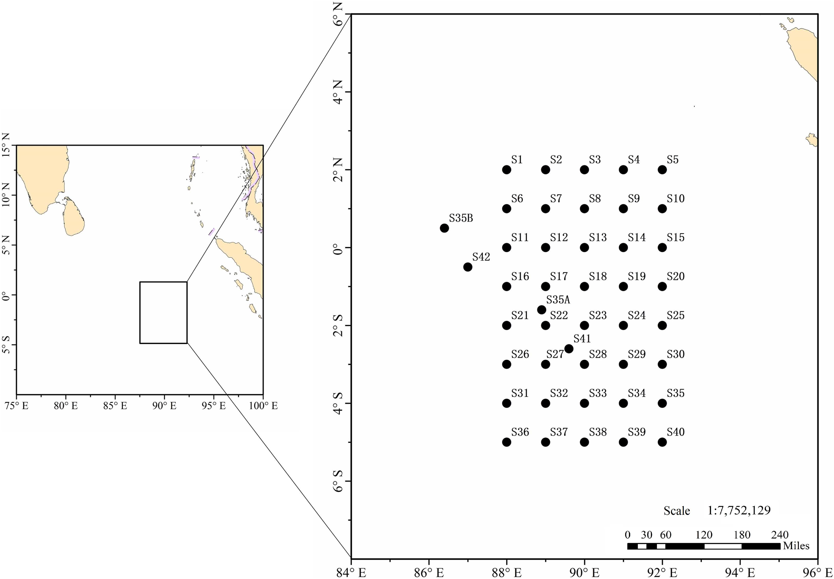
Figure 1. Survey area (Ninety East Ridge) and ichthyoplankton survey stations.

Sample Collection and Processing

Samples were collected by a plankton net (opening diameter of 80 cm, mesh size of 505 μm) with a pre-calibrated flow meter, trawled horizontally for about 10 min at 3 kn (Gaqsiq, 2008). Upon collection ichthyoplankton samples were washed and filtered, and fixed in anhydrous ethanol. Fish eggs and fish larvae were subsequently sorted, identified and counted in the laboratory; taxa were first classified using morphological characteristics (Leis and Carson-Ewart, 2004; Wan and Zhang, 2016), after which one or two individuals (eggs and larvae) at each station were chosen for molecular analysis.

Experimental Methods and Data Analysis

Genetics

A DNA Genome Extraction Kit (TIANGEN Marine Biological Co., Ltd.) was used to extract genomic DNA from eggs and larvae. Concentrations of extracted genomic DNA were measured and then stored in a refrigerator at 4°C prior to genetic assays. Common primers for fish mitochondrial cytochrome oxidase subunit I (COI) gene fragments (F1: 5′-TCAACCAACCACAAAGACATTGGCAC-3′; R1: 5′-TAGACTTCTGGGTGGCCAAAGAATCA-3′) (Ward et al., 2005) were used to amplify the target fragment. The amplicon length was 655 bp. The polymerase chain reaction (PCR) mixture comprised 2.5 μL dNTP (2 mM), 2 μL 10 × Taq buffer (containing Mg²⁺), 1 μL (2 mM) of each F1 and R1 primer, 1 μL DNA template, 0.15 μL Taq DNA polymerase, and double-distilled water to bring the final volume to 25 μL. The PCR program involved a 95°C predenaturation step for 5 min; 30 cycles of 95°C denaturation for 30 s, 52°C annealing for 30 s, and 72°C extension for 30 s; and a 72°C extension for 10 min. A 3 μL sample of PCR amplification product was then separated on a 1.5% agarose gel by electrophoresis, and those products with a concentration sufficiently high for sequencing were sent to Qingdao Personal Gene Biotechnology (Qingdao) for purification and bidirectional DNA sequencing.

All target sequences were first compared with our database constructed based on the catches of the light-liftnet fishing, and then blasted in the NCBI database. Sequences with genetic similarity ≥ 98% were regarded as conspecific, those from 92 to 98% as congeneric, and those from 85 to 92% as confamilial (Ko et al., 2013; Li et al., 2018). To reflect the interspecific relationship, we chosen Carcharhinus longimanus (EU398627 and GU440259) as an outgroup. A neighbor-joining (NJ) tree was created using MEGA 5.0 software based on the best selected K2P model. Genetic distances within species, between species, and between genera were calculated (Tamura et al., 2011).

Dominant Species

The index of relative importance (IRI) was used to identify dominant taxa (Pinkas et al., 1971) in accordance with the formula IRI = M% × F%, where M% represents the percentage of each species relative to the total number of ichthyoplankton samples, and F% is the percentage of stations at which a given species appears. We considered species with an IRI > 200 to be dominant (Zhang et al., 2019).

Species Diversity

The following formulas were used to analyze species diversity (Shannon and Wiener, 1963; Pielou, 1966; Ludwig and Reynolds, 1988):

Margalef’s species richness index:

$$D=S-1/lnN;$$

Shannon–Weiner diversity index:

$$H^{\prime }=-\sum P_{i}ln{P}_i;$$

Pielou’s evenness index:

$$J^{{}^{\prime }}=H^{{}^{\prime }}/lnS.$$

In these equation, S = the total number of species, and P_i the ratio of the number of samples of ichthyoplankton species i to the total number of ichthyoplankton samples, i.e., P_i = n_i/N, where n_i = the number of individuals of species i and N = the total number of ichthyoplankton samples.

Correlating Environmental Variables

Generalized additive model (GAM) was used to analyze the influence of environmental factors on the trends of ichthyoplankton abundance (Hastie and Tibshirani, 1990). Because the distributions of fish eggs and larvae are closely related, we analyze them as a whole in the GAM. Ichthyoplankton abundance at each station was used as a biological indicator; it was log-transformed [Log(AD + 1)] and used as a dependent variable in the model. Our GAM was constructed using the “mgcv” package in R language (R Development Core Team, 2012).

According to net mouth area, trawl speed, trawl time, and numbers of ichthyoplankton caught, we calculated ichthyoplankton abundance per unit volume using AD = $\frac{T}{O\times L\times C\times 100}$, where AD = ichthyoplankton abundance (ind./100 m³), T = number of ichthyoplankton per net (ind.), O = net mouth area (m²), L = flow rate (flow meter), and C = a calibration value of the flow meter.

As all ichthyoplankton samples were collected from sea surface, the selected several environmental variables also come from surface environment, including sea surface temperature (SST), sea surface height (SSH), sea surface salinity (SSS), and sea surface chlorophyll a concentration (Chl a). To visually present the effect of currents on the distributions of ichthyoplankton, we plotted average geostrophic current during the survey period, and superimposed the distribution of ichthyoplankton abundance onto this. SST, SSS, and Chl a were measured on site with a SV48 M probe (German Sea-Sun-Technology), and mean SSH distance and geostrophic flow data (including the variables u and v) were obtained from the National Oceanic and Atmospheric Administration¹ website.

Results

Species Identification and Composition

We successfully amplified 129 sequences (GenBank with access numbers MZ892544∼MZ892597). The 652 bp target fragment base composition comprised T (29.5%), C (28.0%), A (23.4%), and G (19.1%), and had 318 variable sites, 307 parsimony-informative sites, and 11 single-informative sites. With C. longimanus as an outgroup, NJ tree including all sequences (Figure 2) formed 31 groups (including one for C. longimanus) (Supplementary Figure 1). Within-group genetic distances ranged from 0.000 to 0.006, and between-group genetic distances ranged from 0.116 to 0.465 (Supplementary Figure 2 and Supplementary Table 1). These values are generally consistent with the “10× rule” for distance between species, indicating that each group had distinct species.

FIGURE 2

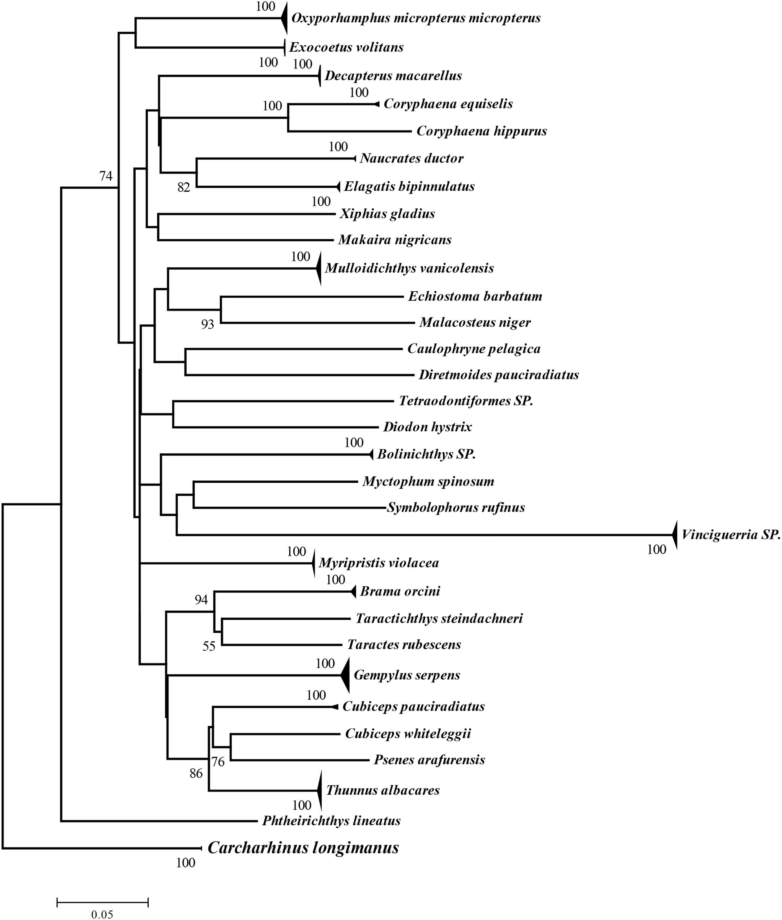
Figure 2. Neighbor-joining phylogenetic tree for surface-dwelling ichthyoplankton from above Ninety East Ridge based on the K2P model.

The NJ tree and genetic distances revealed 30 fish species in the samples. For eggs from which PCR products could not be successfully amplified, we relied upon external morphology for identification. However, because eggs were fixed in ethanol and some taxonomic characteristics were lost, identification of seven taxa was limited to family level. Therefore, 37 species of ichthyoplankton were identified in this survey, belonging to 7 orders, 20 families, and 27 genera (Supplementary Table 2), of which 1 species was identified to order, 7 to family, 1 to genus, and 28 to species. The 16 species represented by larvae belonged to 6 orders, 11 families, and 14 genera, and the 24 species identified from eggs belonged to 5 orders, 14 families, and 16 genera. Only three species (Oxyporhamphus micropterus, Thunnus albacares, Gempylus serpens) were represented by both eggs and larvae.

Most species (11 families, 15 genera, 20 species) belonged to the order Perciformes, followed by Myctophiformes (1 family, 3 genera, 5 species), Beloniformes (2 families, 2 genera, 4 species), Stomiiformes (2 families, 3 genera, 3 species), Beryciformes (2 families, 2 genera, 2 species), Tetraodontiformes (1 family, 1 genus, 2 species), and Lophiiformes (1 family, 1 genus, 1 species).

Species Distribution and Abundance

Of 616 ichthyoplankton samples, 109 were represented by larvae and 507 by eggs. Excluding stations S9 and S25 (where no ichthyoplankton were caught), the number of eggs or larvae (samples) collected at a station ranged from 1 (S39) to 79 (S29) (averaged 14, Figure 3). At 31 stations there were fewer than 20 ichthyoplankton samples, 8 stations with 21–35 samples, and 3 stations with more than 50 samples. Species and numbers of fish eggs and larvae at each station are detailed in Supplementary Table 3. Overall, more ichthyoplankton samples were caught in the central and southern parts of the surveyed sea area.

FIGURE 3

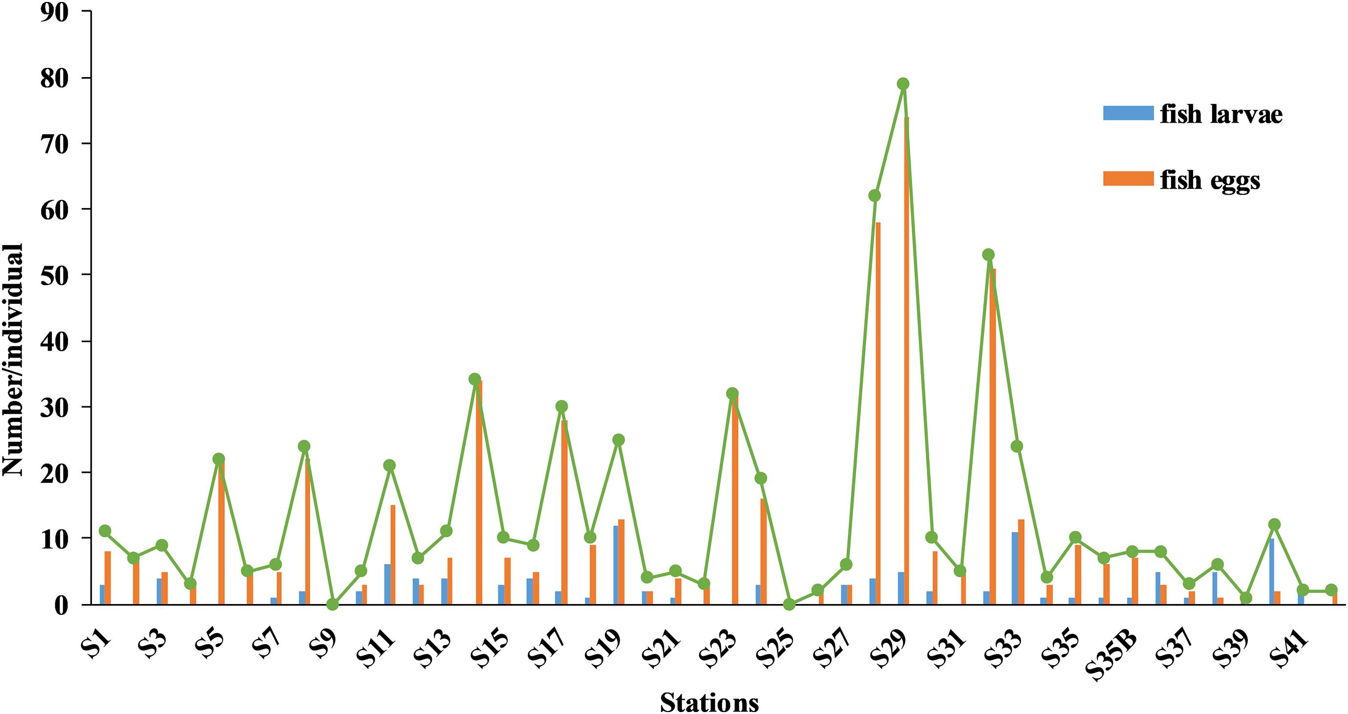
Figure 3. Distributions of fish eggs and larvae, and total numbers of ichthyoplankton caught by stations above Ninety East Ridge.

Ichthyoplankton abundance at each station was low, ranging from 0 to 17.06 ind./100 m³ (Supplementary Figure 3), abundances of 11 stations were < 1 ind./100 m³, 21 stations were 1–3 ind./100 m³, 9 stations were 3–10 ind./100 m³, 3 stations were > 10 ind./100 m³. Abundances of each species ranged from 0.22 to 33.91 ind./100 m³, for 33 species (89.2% in abundance percentage), average abundances were < 0.3 ind./100 m³, only 4 species had abundances ≥ 0.3 ind./100 m³: Brama orcini (0.3), Decapterus macarellus (0.34), O. micropterus (0.37), and Vinciguerria sp. (0.77).

Excluding stations S9 and S25, the number of species caught was low, ranging from 1 to 6 at each station. Only a single species was caught at 4 stations, 2 species were caught at 9 stations, 3 species were caught at 13 stations, 4 species were caught at 8 stations, 5 species were caught at 7 stations, and 6 species were caught at a single (S33) station.

The numbers of individuals per species in all samples combined ranged from 1 to 157. Only a single individual was caught for 13 species (e.g., Makaira nigricans, Caulophryne pelagica, Diretmoides pauciradiatus, Malacosteus niger, Xiphias gladius), whereas 2–20 individuals was caught for of 15 species (e.g., Echiostoma barbatum, Coryphaena equiselis, Diodon hystrix, Naucrates ductor, Exocoetus volitans). For T. albacares, Myripristis violacea, G. serpens, Mulloidichthys vanicolensis, and Exocoetidae sp. 1, 20–45 individuals of each were caught, the numbers of individuals caught of B. orcini, D. macarellus, and O. micropterus were similar. The most abundantly represented taxon was Vinciguerria sp., of which 157 individuals were caught.

The number of stations where each species occurred ranged from 1 to 13. Twenty species (e.g., M. nigricans, C. pelagica, E. barbatum, Taractes rubescens, Symbolophorus rufinus, Coryphaena hippurus, Cubiceps whiteleggii) were caught at only one station; 12 species (e.g., Myctophidae sp. 2, Exocoetidae sp. 1, B. orcini, D. macarellus, M. violacea) were caught at 2–10 stations; 3 species (Vinciguerria sp., T. albacares, and O. micropterus) were caught at 11–12 stations, and 2 species (M. vanicolensis and G. serpens) were caught at 13 stations.

Dominant Species and Species Diversity

Species with an IRI > 200 were considered dominant (Supplementary Table 4), including Vinciguerria sp. (637), O. micropterus (308), and D. macarellus (255); their proportional contributions to total abundance were 25.5, 12.3, and 11.2%, respectively. Moreover, G. serpens, M. vanicolensis, T. albacares, M. violacea, and B. orcini also had high IRI values.

The mean ichthyoplankton Shannon–Weiner diversity index (H’) was 0.83 (0.00–1.52); for two stations with no samples and four stations where only a single species was caught, this diversity index was 0. At 17 (38.63%) stations this index exceeded 1. Average richness index (D) was 1.01 (0.00–2.16), and this index exceeded 1 at 22 (50%) stations. The evenness index (J’) was 0.79 (0.20–1.00) (Supplementary Table 5).

Relationship Between Distribution Characteristics of Ichthyoplankton and Their Environment Variables

The distribution of environmental variables for each station is shown in Supplementary Figure 4. SST values ranged from 27.0 to 29.3°C, with peak ichthyoplankton abundance at about 28.4°C. SSS values ranged from 33.6 to 34.8‰, with peak abundance at about 34.5‰. SSH values ranged from −4.9 to 9.6 cm, with peak abundance at about −2 cm. Chl a values ranged from 0.03 to 0.78 mg/m³, with peak abundance at about 0.15 mg/m³.

Of the four environmental variables, the GAM revealed that only SSH was significantly correlated with ichthyoplankton abundance (P < 0.05). How ichthyoplankton abundance responded to each environmental variable is shown in Figure 4. SSH and abundance were negatively correlated. There were no obvious changes in abundance with SSS between 33.6 and 34.2‰, but abundance was positively correlated with SSS at higher values. SST and Chl a were positively correlated with abundance.

FIGURE 4

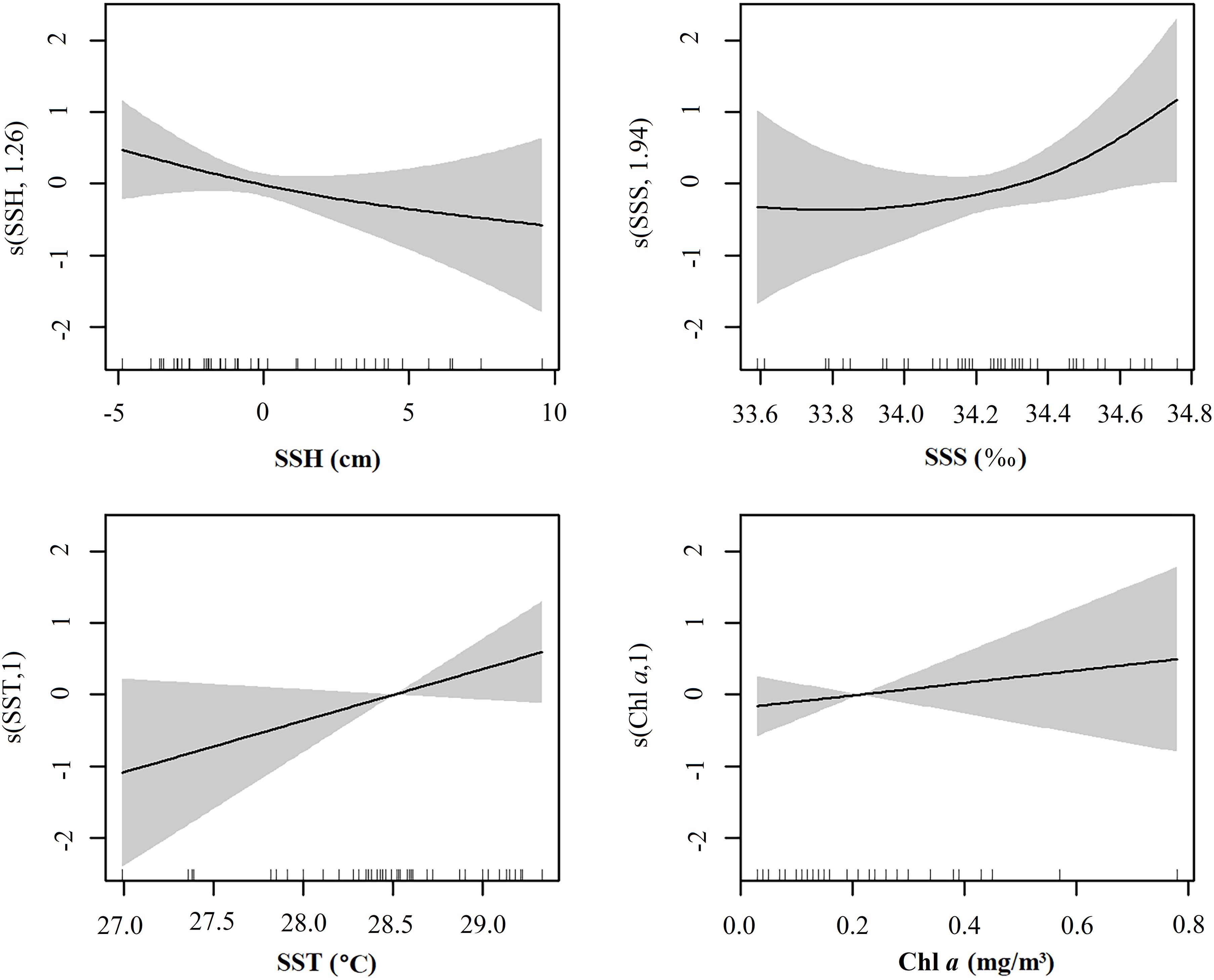
Figure 4. Non-linear responses of ichthyoplankton abundance to environmental variables.

Discussion

Most ichthyoplankton are small and thus are easily overlooked, and have been regarded as a large subset of zooplankton. However, because ichthyoplankton represent an important stage in the life cycles of fish, they are important in assessments of environmental impact, fishery resources, and responses to climate change. Ichthyoplankton also represent an important food source and link in marine food chains; therefore, their identification is important (Shao et al., 2001). Because of their small size, complex external morphology and anatomy, and ontogenetic variability, the characters used to visually identify ichthyoplankton are few and difficult to observe, hampering identification. We augmented our morphological identifications with DNA barcoding—a technique that has been successfully applied in other ichthyoplankton studies (Zhou et al., 2015; Ahern et al., 2018; Duke and Burton, 2020)—to improve the accuracy of our identifications.

We used DNA barcoding to identify 27 taxa to species, two species to genus, and one species to order. Of the 37 taxa identified in samples, 24 species were not collected during a field survey of pelagic fishery resources (unpublished data). Identified species included oceanic migrators (M. nigricans), nearshore species (D. hystrix), uncommon species (Phtheirichthys lineatus), common Exocoetidae species (O. micropterus), and deep-ocean species (M. niger, D. pauciradiatus, E. barbatum, C. pelagica). Among the 10 taxa not identified to species, Vinciguerria sp. (family Phosichthyidae) was most abundant (25.5% of all identified specimens), suggesting a potential resource exists in or near the surveyed sea area. Tetraodontiformes sp., a suspected cryptic species of Tetraodontiformes, was also detected. Our results confirm the effectiveness of DNA barcoding for ichthyoplankton identification; this technique can increase the known diversity and richness of species in an area and provide a scientific reference for studies on variation in fisheries. Because both the abundance of individuals at each station and the number of species was low (only four species at three stations had abundances that exceeded 10 ind./100 m³), the surveyed area might not be a main spawning area, or autumn might not be a main spawning period for most of these fish species.

The H′ for the surveyed area was lower than that for continental shelf and adjacent east Indian Ocean (Holliday et al., 2012; Beckley et al., 2019; Rathnasuriya et al., 2021), perhaps because that the nearshore sea area has relatively high habitat diversity, rich productivity, and bait resources, and is a spawning and breeding ground for many fishes (Holliday et al., 2012). Meanwhile, the surveyed sea area was located in the open ocean and presented a single habitat and complex ocean currents; most involved species are oceanic migratory fish, or few nearshore species transported by ocean currents.

The temporal and spatial distributions of ichthyoplankton are affected by broodstock reproductive characteristics, and the environment, mainly Chl a, temperature, salinity, depth, and ocean currents (Zheng et al., 2003; Xiao et al., 2017). Our GAM model revealed that ichthyoplankton in the surveyed area were concentrated in areas of low SSH and high SSS, SST, and Chl a (Figure 3), with SSH most strongly correlated with ichthyoplankton abundance. In contrast, the distributions of nearshore ichthyoplankton are mainly affected by other variables such as Chl a (Zhang et al., 2019), SSS (Chen et al., 2015), SST, and water depth (Li et al., 2017; Xiao et al., 2017; Chermahini et al., 2021).

Water temperature strongly affects fish spawning and egg development, with high temperatures possibly stimulating both. Fish larval species richness and total abundance increases with water temperature, with species being replaced over time, assisted by increased prey as a consequence of increased water temperature (Meinert et al., 2020). However, our surveyed area is relatively large, and changes in water temperature are relatively small, with maximum SST differences of 2.3°C between stations, and with 75% of stations having SSTs between 28.3 and 29°C. Thus, not surprisingly, we report a low correlation between SST and ichthyoplankton abundance in our GAM.

In addition to seeking suitable water temperatures for survival, marine fishes must find places with better conditions for feeding when migrating. High Chl a can improve ocean primary productivity, increasing the probability of fish feeding, and inducing their aggregation. We assume that the spawning probability of aggregating fishes in these environments is increased, which is why we included Chl a in our analyses. However, our GAM did not show a high correlation between Chl a concentration and fish abundance. Additionally, ichthyoplankton abundance and total species richness at each station (unpublished data) were not obviously correlated either, indicating that areas with many captured individuals may not have more ichthyoplankton.

Variation in SSH is generally caused by a shift in the direction of ocean currents, with low SSHs more often found near where ocean currents change direction or vortices occur (Bakun, 2006; Tittensor et al., 2010; Prants et al., 2014). The average geostrophic flow vector diagram for the survey period revealed that stations S28 and S29 (with the highest ichthyoplankton abundances) are in areas where large ocean currents meander. Vortices forming low SSHs not only gather and passively transport ichthyoplankton, but also increase their feeding opportunities and survival rate (Meinert et al., 2020). Despite this, SSH alone does not adequately explain the distributions of ichthyoplankton across the surveyed sea area, indicating that their abundance is influenced by other variables, such as ocean currents, illuminance, total nitrogen, total phosphorus, pH, suspended matter, dissolved oxygen, and/or chemical oxygen demand (Chen et al., 2015).

The oceanic marine environment is changeable, and ichthyoplankton in different sea areas are affected by different variables, even giving rise to multivariable synergistic effects. Therefore, to truly understand species composition, quantity distribution, and the relationships between ichthyoplankton and environmental variables around the Ninety East Ridge, additional samples collected at different times of the year and more environmental data are needed. Various models could be used to comprehensively analyze biological and environmental data to provide further empirical support for studies on the variation in and development and utilization of fishery resources in this area.

Data Availability Statement

The datasets presented in this study can be found in online repositories. The names of the repository/repositories and accession number(s) can be found in the article/Supplementary Material.

Ethics Statement

The animal study was reviewed and approved by the Ethics Committee of the Laboratory of Animal Welfare and Ethics of Shanghai Ocean University.

Author Contributions

LZ performed the data analysis and wrote the manuscript. SL, RW, and XM assisted with GMA model analysis. JZ and JX assisted with molecular analysis. LL and PS conceived and designed the study, and critically revised the manuscript. All authors listed in this manuscript have made a direct and substantial contribution to this work.

Funding

This research was funded by the National Programme on Global Change and Air–Sea Interaction (GASI-01-EIND-YD01aut/spr).

Conflict of Interest

The authors declare that the research was conducted in the absence of any commercial or financial relationships that could be construed as a potential conflict of interest.

Publisher’s Note

All claims expressed in this article are solely those of the authors and do not necessarily represent those of their affiliated organizations, or those of the publisher, the editors and the reviewers. Any product that may be evaluated in this article, or claim that may be made by its manufacturer, is not guaranteed or endorsed by the publisher.

Acknowledgments

The present study could not have been performed without assistance from Liangming Wang, Cheng Liu, Zizi Cai, and Yuanyuan Li during experimentation and data processing. We also thank the editors and reviewers of this manuscript for their constructive comments.

Supplementary Material

The Supplementary Material for this article can be found online at: https://www.frontiersin.org/articles/10.3389/fmars.2021.764859/full#supplementary-material

Footnotes

1. ^ https://www.ngdc.noaa.gov/

References

Ahern, A., Gomez-Gutierrez, J., Aburto-Oropeza, O., Saldierna-Martinez, R. J., Johnson, A. F., Harada, A. E., et al. (2018). DNA sequencing of fish eggs and larvae reveals high species diversity and seasonal changes in spawning activity in the southeastern Gulf of California. Mar. Ecol. Prog. Ser. 592:12446. doi: 10.3354/meps.2018.12446

CrossRef Full Text | Google Scholar

Bakun, A. (2006). Fronts and eddies as key structures in the habitat of marine fish larvae: opportunity, adaptive response and competitive advantage. Sci. Mar. 70, 105–122. doi: 10.3989/SCIMAR.2006.70S2105

PubMed Abstract | CrossRef Full Text | Google Scholar

Beckley, L. E., Holliday, D., Sutton, A. L., Weller, E., Olivar, M. P., and Thompson, P. A. (2019). Structuring of larval fish assemblages along a coastaloceanic gradient in the macro-tidal, tropical Eastern Indian Ocean. Deep Sea Res. Part II Top. Stud. Oceanogr. 161, 105–119. doi: 10.1016/J.DSR2.2018.03.008

CrossRef Full Text | Google Scholar

Chen, Y. G., Mao, C. Z., Zhong, J. S., and Xu, Z. L. (2015). Influence of abiotic factors on spatiotemporal patterns of larval fish assemblages in the surf zones of the Yangtze River estuary and Hangzhou Bay. J. Fish. Sci. China 22, 780–790. doi: 10.3724/SP.J.1118.2015.140392

CrossRef Full Text | Google Scholar

Chermahini, A. M., Shabani, A., Naddafi, R., Ghorbani, R., Rabbaniha, M., and Noorinejad, M. (2021). Diversity, distribution, and abundance patterns of ichthyoplankton assemblages in some inlets of the northern Persian Gulf. J. Sea Res. 167:101981. doi: 10.1016/j.seares.2020.101981

CrossRef Full Text | Google Scholar

Duke, E. M., and Burton, R. S. (2020). Efficacy of metabarcoding for identification of fish eggs evaluated with mock communities. Ecol. Evol. 10, 3463–3476. doi: 10.1002/ECE3.6144

PubMed Abstract | CrossRef Full Text | Google Scholar

Ellis, T., and Nash, R. (1997). Predation by sprat and herring on pelagic fish eggs in a plaice spawning area in the Irish Sea. J. Fish Biol. 50, 1195–1202. doi: 10.1111/J.1095-8649.1997.TB01647.X

CrossRef Full Text | Google Scholar

Gaqsiq (2008). GB/T 12763.6-2007, Specification of Oceanographic Investigation – Part 6: Marine Biological Investigation. Beijing: Standards Press of China.

Google Scholar

Hastie, T. J., and Tibshirani, R. J. (1990). Generalized additive models. Stat. Sci. 1, 297–310. doi: 10.2307/2532174

CrossRef Full Text | Google Scholar

Holliday, D., Beckley, L. E., Millar, N., Olivar, M. P., Slawinski, D., Feng, M., et al. (2012). Larval fish assemblages and particle back-tracking define latitudinal and cross-shelf variability in an eastern Indian Ocean boundary current. Mar. Ecol. Prog. Ser. 460, 127–144. doi: 10.3354/MEPS09730

CrossRef Full Text | Google Scholar

Ko, H. L., Wang, Y. T., Chiu, T. S., Lee, M. A., Leu, M. Y., Chang, K. Z., et al. (2013). Evaluating the accuracy of morphological identification of larval fishes by applying DNA barcoding. PLoS One 8:e53451. doi: 10.1371/journal.2013.pone.0053451

CrossRef Full Text | Google Scholar

Leis, J. M., and Carson-Ewart, B. M. (2004). The Larvae of Indo-Pacific Coastal Fishes: A Guide to Identification (Fauna Malesiana handbook 2), 2nd Edn. Leiden: Brill.

Google Scholar

Li, Y., Sun, P., and Yuan, C. (2019). Phytoplankton assemblage and their inter-annual variation in the south sector of eastern Indian Ocean in spring. Mar. Environ. Sci. 38, 825–832.

Google Scholar

Li, Y., Zhang, L., Song, P., Zhang, R., Wang, L., and Lin, L. (2018). Fish diversity and molecular taxonomy in the Prydz bay during the 29th CHINARE. Acta Oceanol. Sin. 37, 15–20. doi: 10.1007/S13131-018-1228-Y

CrossRef Full Text | Google Scholar

Li, Z. G., Ye, Z. J., Wan, R., Chen, Y., Tian, Y. J., Ren, Y. P., et al. (2017). Evaluating the relationship between spatial heterogeneity and temporal variability of larval fish assemblages in a coastal marine ecosystem (Haizhou bay, China). Mar. Ecol. 38:e12446. doi: 10.1111/maec.2017.12446

CrossRef Full Text | Google Scholar

Ludwig, J. A., and Reynolds, J. F. (1988). Statistical Ecology: A Primer in Methods and Computing. Hoboken: John Wiley & Sons.

Google Scholar

Meinert, C. R., Clausen-Sparks, K., Cornic, M., Sutton, T. T., and Rooker, J. R. (2020). Taxonomic richness and diversity of larval fish assemblages in the oceanic Gulf of Mexico: links to oceanographic conditions. Front. Mar. Sci. 7:579. doi: 10.3389/fmars.2020.00579

CrossRef Full Text | Google Scholar

Pielou, E. C. (1966). The use of information theory in the study of ecological succession. Theor. Biol. 10, 370–383. doi: 10.1016/0022-5193(66)90133-0

CrossRef Full Text | Google Scholar

Pinkas, L., Oliphant, M. S., and Iverson, I. L. K. (1971). Food habits of albacore, bluefin tuna, and bonito in California waters. Fish. Bull. 52, 11–46.

Google Scholar

Prants, S. V., Budyansky, M. V., and Uleysky, M. Y. (2014). Identifying lagrangian fronts with favourable fishery conditions. Deep Sea Res. Part I. Ocean. Res. Pap. 90, 27–35. doi: 10.1016/J.DSR.2014.04.012

CrossRef Full Text | Google Scholar

R Development Core Team (2012). A Language and Environment for Statistical Computing. Vienna: R Foundation for Statistical Computing.

Google Scholar

Rathnasuriya, M. I. G., Mateos-Rivera, A., Skern-Mauritzen, R., Wimalasiri, H. B. U., Jayasinghe, R. P. P. K., Krakstad, J. O., et al. (2021). Composition and diversity of larval fish in the Indian Ocean using morphological and molecular methods. Mar. Biodivers. 51:39. doi: 10.1007/s12526-021-01169-w

CrossRef Full Text | Google Scholar

Shannon, C. E., and Wiener, W. (1963). The Mathematical Theory of Communication. Urbana: University of Illinois Press.

Google Scholar

Shao, K. T., Yang, J. S., and Chen, K. C. (2001). An Identification Guide of Marine Fish Eggs from Taiwan. Taipei: Boyu Professional Document Processing Center.

Google Scholar

Tamura, K., Peterson, D., Peterson, N., Stecher, G., Nei, M., and Kumar, S. (2011). MEGA5: molecular evolutionary genetics analysis using maximum likelihood, evolutionary distance, and maximum parsimony methods. Mol. Biol. Evol. 28, 2731–2739. doi: 10.1093/MOLBEV/MSR121

PubMed Abstract | CrossRef Full Text | Google Scholar

Tittensor, D. P., Mora, C., Jetz, W., Lotze, H. K., Ricard, D., Berghe, E. V., et al. (2010). Global patterns and predictors of marine biodiversity across taxa. Nature 466, 1098–1101. doi: 10.1038/nature09329

PubMed Abstract | CrossRef Full Text | Google Scholar

Wan, R. J., and Zhang, R. Z. (2016). Fish Eggs, Larvae and Juveniles in the Offshore Waters of China and Their Adjacent Waters. Shanghai: Shanghai Scientific and Technical Publishers.

Google Scholar

Wang, J., Kan, J., Borecki, L., Zhang, X., Wang, D., and Sun, J. (2016). A snapshot on spatial and vertical distribution of bacterial communities in the eastern Indian Ocean. Acta Oceanol. Sin. 35, 85–93. doi: 10.1007/S13131-016-0871-4

CrossRef Full Text | Google Scholar

Wang, X., Li, C., Liu, K., Zhu, L., and Li, D. (2020). Atmospheric microplastic over the South China Sea and East Indian Ocean: abundance, distribution and source. J. Hazard. Mater. 389:121846. doi: 10.1016/j.jhazmat.2019.121846

PubMed Abstract | CrossRef Full Text | Google Scholar

Ward, R., Zemlak, T., Innes, B., Last, P., and Hebert, P. (2005). DNA barcoding Australia’s fish species. Philos. Trans. R. Soc., B. 360, 1847–1857. doi: 10.1098/RSTB.2005.1716

PubMed Abstract | CrossRef Full Text | Google Scholar

Wei, H. L., Fang, N. Q., Ding, X., Nie, L. S., and Liu, X. M. (2007). Major environmental events reflected by pelagic records since 3.5 Ma BP in the Ninetyeast ridge at the equator. Geol. Bull. 26, 1627–1632. doi: 10.1016/S1872-5791(08)60002-0

CrossRef Full Text | Google Scholar

Wei, Y., Zhang, G., Chen, J., Wang, J., Ding, C., Zhang, X., et al. (2019). Dynamic responses of picophytoplankton to physicochemical variation in the eastern Indian Ocean. Ecol. Evol. 9, 5003–5017. doi: 10.1002/ECE3.5107

PubMed Abstract | CrossRef Full Text | Google Scholar

Xiao, H. H., Zhang, C. L., Xu, B. D., Xue, Y., and Ren, Y. P. (2017). Spatial pattern of ichthyoplankton assemblage in the coastal waters of central and southern Yellow Sea in spring. Acta Oceanol. Sin. 39, 34–47. doi: 10.3969/j.issn.0253-4193.2017.08.004

CrossRef Full Text | Google Scholar

Zhang, H., Xian, W., and Liu, S. (2019). Seasonal variations of the ichthyoplankton assemblage in the Yangtze estuary and its relationship with environmental factors. Peer J 7:e6482. doi: 10.7717/peerj.2019.6482

CrossRef Full Text | Google Scholar

Zhao, C. Y., and Zhang, R. Z. (1985). Fish Eggs and Larvae in China Seas. Shanghai: Shanghai Scientific and Technical Publishers.

Google Scholar

Zheng, Y. J., Chen, X. Z., and Cheng, J. H. (2003). The Biological Resources and Environment in the East China Sea Continental Shelf. Shanghai: Shanghai Scientific and Technical Publishers.

Google Scholar

Zhou, M. Y., Chen, X., and Yang, S. Y. (2015). Identification of several fish eggs and larvae by DNA barcoding in Xiamen water. Mar. Environ. Sci. 34, 120–125.

Google Scholar