 Tae-Kon Kim
 Changbin Lim1
- 1School of Civil, Architectural and Environmental System Engineering, Sungkyunkwan University, Suwon, South Korea
- 2Graduate School of Water Resources, Sungkyunkwan University, Suwon, South Korea
Recently, because of the influence of climate change on sea level change, there has been growing concern regarding the erosion of beaches, which play a role in reducing the damage caused by coastal disasters. However, despite these concerns, a comprehensive understanding of the morphodynamic relationship between hazard factors and beach erosion is still lacking. Therefore, in this study, a vulnerability analysis of beach erosion was conducted by applying the shoreline response model (SLRM) of bulk model type, which identifies the physical characteristics of relevant coefficients based on the suspended sediment movement processes. To characterize wave energy incidence, storm wave scenario modeling and extreme wave analysis were conducted using wave data of 40 years on the east coast of Korea provided by the National Oceanic and Atmospheric Administration. A dimensionless mathematical function representing the storm wave scenario was proposed as a function of the peak wave height. In addition, to examine whether the beach vulnerability curve (BVC) obtained from the SLRM is valid, it was compared with the long-term shoreline observation data conducted at Maengbang Beach. For the past 9 years, sand sampling and shoreline observations were performed at Maengbang Beach about 5 times a year. However, since observations were performed in time intervals of several months, the direct comparison with model results was impossible, so a comparative analysis through statistical analysis of shoreline variability was performed. The variability of the shoreline for each reference point followed a normal distribution with a standard deviation of approximately 7.1 m. As a result of comparing the BVC results obtained from these statistical characteristics with those obtained from the model, significant similarity was shown in the high wave condition. Finally, the model was performed on two factors (mean wave height and peak wave height) which appear in SWSF and three factors (wave energy at breaking point, beach response factor and beach recovery factor) which appear in SLRM, and by analyzing the results, an approximate formula for the BVC is derived. This novel BVC approximation equation provides an intuitive understanding of the factors that affect beach vulnerability as well as their importance, and estimates the beach buffer section required to prevent coastal facilities from being damaged by erosion during a specific period. The results of this study can help limit reckless coastal development and mitigate erosion damage.
Introduction
Numerous research efforts have been made, including establishing concepts and developing models, to evaluate the vulnerability of the coastal environment in relation to coastal disasters and climate change (IPCC, 1996, 2001; UKCIP, 2003; UNDP, 2005; UNFCCC, 2005; Han, 2006; Yook et al., 2011). Although studies often define vulnerability differently, in general, it can be characterized to be receiving a certain amount of impact from external pressure. In particular, the erosion vulnerability of coastal areas, which are prone to coastal disasters because of the effects of climate change, such as sea level changes, is emerging as a research topic of interest. However, despite these efforts, a comprehensive understanding of the hazard factors related to beach erosion and the morphodynamic processes of shoreline retreat is lacking for evaluating beach vulnerability.
Most of the understanding of episodic erosion phenomena is based on statistical analysis of beach erosion survey data or numerical model results that rely on physical parameters related to the sediment process (Mendoza and Jimeńez, 2006; Bosom and Jimeńez, 2011; Oliveira et al., 2014; Ballesteros et al., 2017; Narra et al., 2019; Anfuso et al., 2021). Data analysis has been mainly used for the purpose of finding long-term erosion rates, and short-term erosion has recently become possible with the analysis of CCTV image data. Yates et al. (2009) estimated the convergence position of the shoreline by examining changes in the beach profile as a response to changes in the incoming wave energy via long-term field measurements. In this scenario, if the external hazard is regarded as incoming wave energy and the impact factor is shoreline retreat, the beach vulnerability can be studied. However, their research was limited because the location of the shoreline that ultimately converges when a specific wave energy value was continuously applied. Recently, Park et al. (2019) suggested a methodology for analyzing beach vulnerability by analyzing shoreline data variability observed on the east coast of Korea and the extreme behavior of incident waves. However, the methodology has not been verified because of a lack of long-term wave and shoreline survey data for comparison.
To compensate for these limitations, a method that can quantitatively evaluate beach vulnerability by applying a highly reliable numerical model is required. However, the incidence of wind waves from distant seas to the shore shows an infinitely repeating phenomenon and irregular changes. Therefore, ensuring the reliability of the numerical model is important, and it is also necessary to establish a wave scenario model that considers the characteristics of wave duration. Furthermore, it is necessary to analyze how the duration of the incident wave affects shoreline fluctuations. Specifically, it is necessary to develop a methodology for extracting a vulnerability curve by analyzing long-term wave data and reflecting the influence of the wave duration to determine the maximum receding width of the shoreline. Unlike the wave input conditions used for designing port facilities, the beach response assumes that erosion proceeds according to the incidence of high waves, and when the waves calm, it recovers to its original position. However, there are few cases in which scenario models have been constructed for this purpose. Therefore, in this study, using 40-year National Oceanic and Atmospheric Administration (NOAA) data for the east coast of Korea, a scenario model formula of incident wave height and duration that is dimensionless to the maximum wave height was derived.
Several models have been developed to numerically simulate beach profile responses to identify the causes and develop preventive responses to beach erosion problems caused by storm wave incidence (Larson et al., 1999; Lesser et al., 2004; Roelvink et al., 2009; Deltares, 2018a,b). A shoreline response model of bulk model type was first proposed by Wright et al. (1985a,b). It was used to represent the rate at which the beach state changes and applied the convergence characteristics of beach conditions following storm events in situations where the mechanism of sediment movement in the breaking zone had not yet been elucidated. Later, this equation was also employed for sandbar evolution (Plant et al., 1999) and beach slope change (Madsen and Plant, 2001). Approximately 20 years later, Miller and Dean (2004) proposed a simple governing equation of the ODE type that, based on empirical evidence, relates shoreline change to shoreline position. This equation was calibrated using periodic shoreline data.
The proposed governing equations reveal that the shoreline approaches the equilibrium form for steady-state conditions at approximately exponential rates, which is consistent with laboratory investigations (Swart, 1974) and numerical results (Kriebel and Dean, 1985; Larson et al., 1999). In addition, the recent researches (Yates et al., 2009; Davidson et al., 2013; Toimil et al., 2017) established or examined a shoreline response model using long-term field observations to evaluate its practical applicability. In this study, the ODE type model proposed by Lim et al. (2021) was employed, which derived a correlation of 74% with respect to the wave input and shoreline change observation data used for the blind test of Montaño et al. (2020). Overall, two main constants are employed, the beach response factor and the beach recovery factor, and their physical properties are analyzed by evaluating the horizontal behavior of suspended sediments. However, the peak erosion width indicating the degree of beach erosion vulnerability has not been presented due to the various conditions of wave incidence yet even though the parameters ar and kr of the SLRM related to the beach property of erosion vulnerability are determined.
The main objective of this study is to obtain a relational expression for the vulnerability of the shoreline to episodic erosion according to the impact of storm wave energy given as a function of the peak wave height. Figure 1 shows the detailed research process of applying the SLRM. Section “Extraction of Storm Wave Scenario from NOAA Wave Data” introduces the process of extracting a storm wave scenario function (SWSF) by analyzing NOAA wave data for Maengbang Beach on the east coast of Korea. Section “Derivation of Beach Vulnerability Curve by the Shoreline Response Model” presents a method for deriving the vulnerability curve equation by applying this scenario function to the ODE SLRM, which has been recently proven to exist high reliability. In Section “Beach Vulnerability Curve for Maengbang Beach,” in order to analyze the feasibility of this method, the dependence of beach erosional width on wave frequency was obtained using the results of periodic shoreline surveys. In addition, the results of erosion vulnerability are presented in combination with the extreme wave analysis, which corresponds to the most fundamental vulnerability analysis method, and are compared with the results obtained from the SLRM. In Section “Discussion,” the effect of duration on erosion vulnerability was discussed by modulating the duration of the SWSF. An approximate formula for erosion vulnerability was also developed by analyzing the influence of factors on erosion vulnerability. Finally, the main conclusions are presented and future research paths are proposed based on the results of this study.
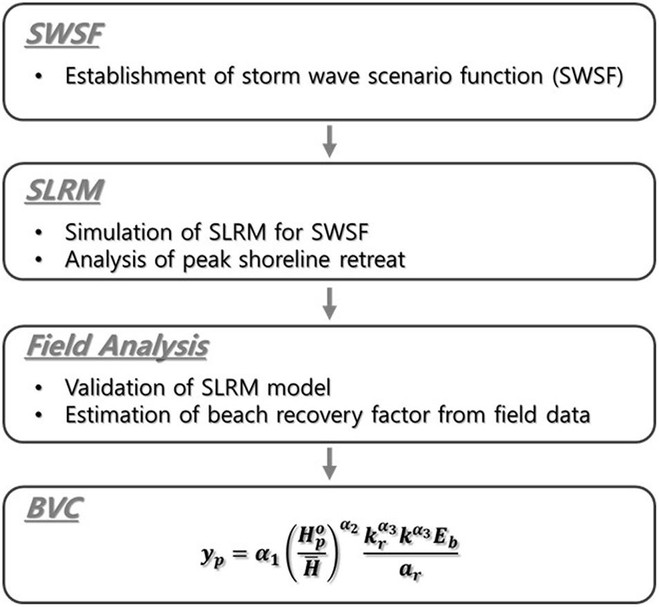
Figure 1. Research processes for deriving a beach vulnerability curve (BVC).
Extraction of Storm Wave Scenario From NOAA Wave Data
Study Site
Maengbang Beach, located in Samcheok City, Gangwondo, on the east coast of South Korea, is a linear coast stretching over approximately 4.6 km in the northwest to southeast (NE-SE) direction. The average beach width is approximately 48.0 m, and the shoreline has a mixture of straight and bow shapes. Maengbang Beach is a sandy beach near Osipcheon and Maeupcheon (Supplementary Figure 1). Supplementary Figure 2 shows its tide table and wave rose diagram (Ministry of Ocean and Fisheries, 2017). The study site has a small spring tidal range of 15.6 cm and total tidal range 33.4 cm with little tidal fluctuation, and the annual mean wave incidence at the study site has a significant wave height of 1.14 m and a significant wave period of 7.78 s. The main wave direction in the deep sea shows 39.5°, and compared to the shoreline inclination angle of about 42°, there is a possibility of net littoral drift to the south.
National Oceanic and Atmospheric Administration Wave Data
For the duration of wave actions, wave influence is reflected in the change of beach profiles and most storm waves show a tendency to develop, peak, and then decrease (Corbella and Stretch, 2012). In this study, wave data from NOAA was used for the storm wave scenario model analysis. The annual changes in the significant wave height and significant wave period of Maengbang Beach from 1979 to 2018 are shown in Supplementary Figures 3,4, respectively. Supplementary Figure 5 is a graph showing the annual change of annual mean significant wave height, peak period, and dominant wave direction. Supplementary Figures 5A,B show the annual variations of values corresponding to 10% intervals from 10 to 90% from the smallest value out of about 365 × 8 (2920) data every year using wave height and period data at 3 h intervals for 40 years. And Supplementary Figure 5C shows the values corresponding to 10% intervals from 10% to 40% in the +/− direction based on 34°N using the wave direction data, showing the change by year for 40 years. It can be seen that the annual mean wave height, period, and wave direction over the past 40 years has been maintained without significant change. Therefore, the amount of long-term change in the wave environment is negligible, and the effect of climate change in this sea area can be found to be very insignificant.
The wave height-period joint probability distribution obtained from the significant wave height-peak period data for these 40 years is shown in Supplementary Figure 6, and the corresponding spectrum is shown in Figure 2. The frequency spectrum was obtained using the joint distribution by converting the period into frequency (Sorensen, 1993) and wave height into spectrum. The directional spectrum is shown in Figure 3. Also, Figures 2, 3 show the dotted line results of the spectrum and wave direction distribution obtained at intervals of every 10 years. The peak frequency is 0.12 Hz, and the incoming deep-sea wave direction showing the peak wave energy was calculated to be 25° clockwise from true north.
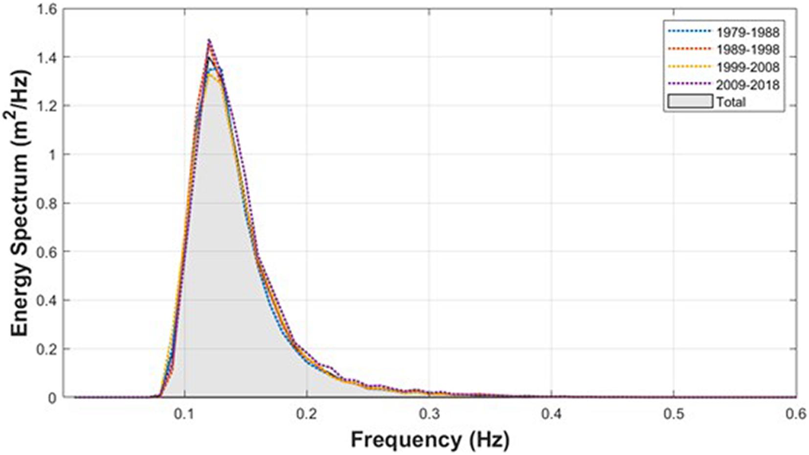
Figure 2. Annual mean wave spectrum at Maengbang coast obtained from the NOAA dataset (1979–2018).

Figure 3. Wave direction distribution at Maengbang coast from the NOAA dataset (1979–2018).
Analysis of Temporal Evolution of Wave Scenario
In order to reproduce the storm wave scenario for Maengbang Beach, the method proposed by Kim et al. (2021) is adopted in this study. Using 40-year NOAA data (38.5°N, 129.0°E) for Bongpo Beach, located about 111 km north of Maengbang Beach, Kim et al. (2021) normalized the wave height and period data to peak wave height values and the time scale as a function of peak wave height. Therefore, the storm scenario for Maengbang Beach was reproduced similarly using 40-year wave data of NOAA grid point (37.5°N, 129.5°E) closest to Maengbang Beach.
Supplementary Figures 7, 8 show the wave height and wave period scenarios, respectively. The dotted lines indicate the mean and maximum values of all storm wave conditions exceeding a peak wave height in deep water () of 4.5 m. The results show that the curves have a good fit with the extreme wave scenario of the NOAA data. In addition, the scenario function of the storm wave height affecting Maengbang Beach is expressed in terms of dimensionless time t′, as given in Eq. 1.
Where AH = 1.28× 10⁻⁹, BH = 0.00007, and . The scenario function of the storm wave period can be expressed as:
Where AT = 4.1×10⁻⁷, BT = 0.0042, and . The time is converted to days from the dimensionless time t according to the peak height (m) as follows:
Supplementary Figure 9 compares the time series data wherein the peak wave height and time are dimensionless for wave scenarios with peak wave heights ranging from 4.5 to 7.5 m. These values were obtained using Eq. 1. Similarly, Supplementary Figure 10 compares the time series data wherein the wave period is dimensionless for wave scenarios with a similar range for peak wave heights. These values were obtained using Eq. 2. The dimensionless time is converted to the real time (day) via multiplication with 365.
Wave Energy at Breaking Point
To apply the SWSF to the SLRM, it is necessary to calculate the wave height at the breaking point using the offshore wave information. If waves are induced in deep water via wave refraction and wave shoaling and they are broken near shore, the height Hb at the breaking point can be obtained according to the law of conservation of energy. In a linear coastal terrain, wherein the isochore line is parallel to the shoreline, assuming that waves break in the shallow water, Eq. 1 can be rearranged in terms of Hb to obtain the following:
Then, by substituting hb = Hb/γ, where γ is the wave breaking coefficient, the relationship can be reorganized as:
where the wave breaking coefficient γ is assumed to be 0.55, which is the generally applied value for significant wave heights. The wave direction θb at the breaking point (assumed to be in shallow water) was obtained by applying Snell’s law as follows:
This effect of refraction is neglected when calculating the breaking wave height, which is the input data of SLRM, from the SWSF of deep sea waves, but Eq. 6 is applied when performing the extreme value analysis on the breaking wave height in Section “Extreme Wave Height Analysis of Incidence Waves”. Figure 4 shows the wave scenario functions determined using the peak wave height in deep water for the real-time scale treal and the corresponding wave energy at the breaking point.
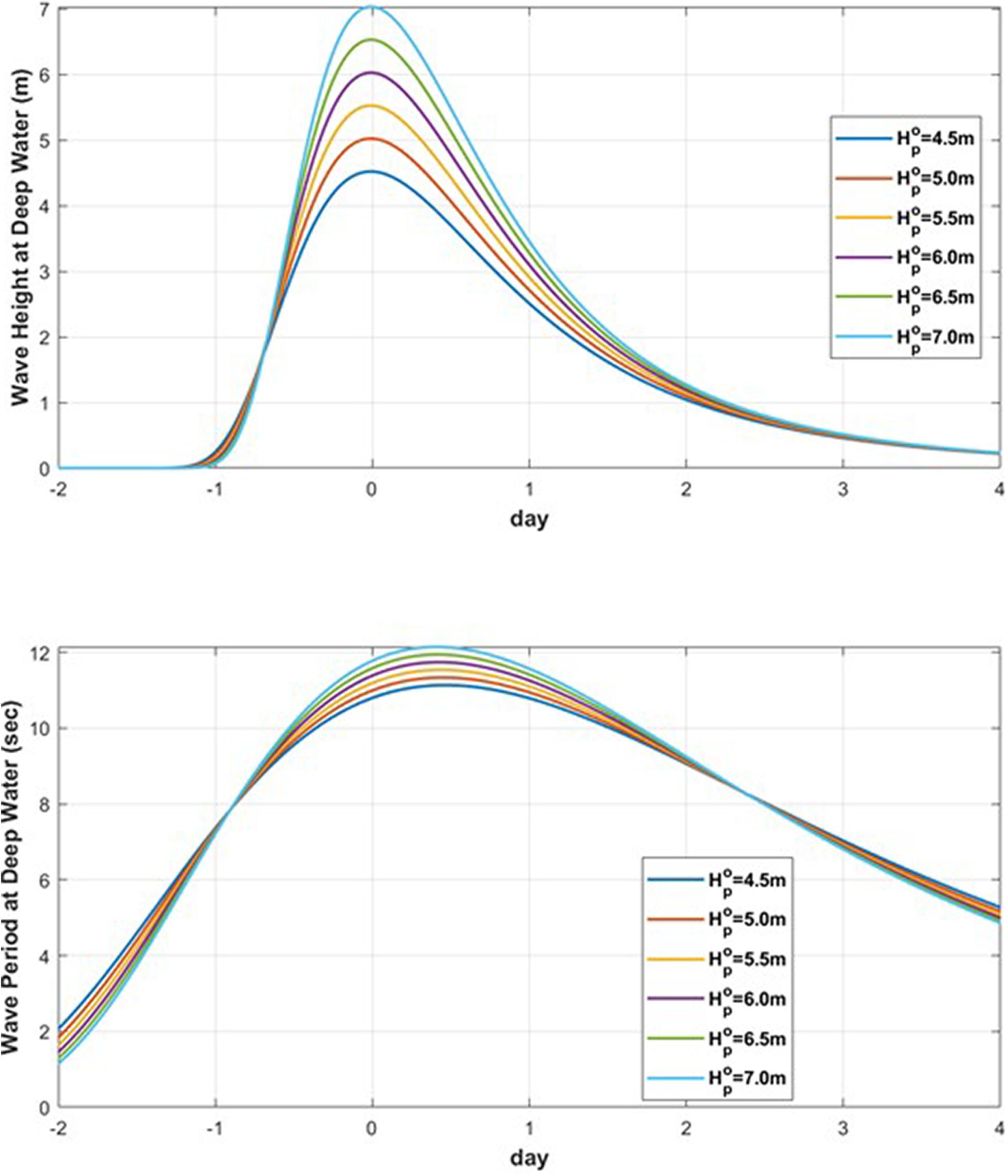
Figure 4. Temporal variation of storm wave height (Up) and wave period (Down) in deep water with respect to .
Derivation of Beach Vulnerability Curve by the Shoreline Response Model
Governing Equation of the Shoreline Response Model
The governing equation used to determine the maximum retreat width of the shoreline as an indicator of erosion vulnerability is given by Eq. 7. This equation was empirically obtained by Miller and Dean (2004), and recently physical validity has been verified by Lim et al. (2021) by using the horizontal behavior concept of suspended sediment. In addition, applying about 11 years of wave input data (via model prediction) and shoreline data (via CCTV analysis) provided by Montaño et al. (2020), Lim et al. (2021) achieved satisfactory model performance showing a 74% correlation.
where y is the shoreline erosion width and kr is the beach recovery factor, which is related to the recovery speed at which the suspended sediment returns to its original position after erosion. Further, Eb is the energy at the breaking point for the wave scenario model described in Subsection “Analysis of Temporal Evolution of Wave Scenario,” and ar is the beach response factor, which is a positive value in Eq. 7, and its value can be obtained from the sedimentation trend curve equation presented by Yates et al. (2009) or simply from D50, as suggested by Kim and Lee (2018).
Estimating Beach Response and Recovery Factors
Two physical parameters exist in the shoreline response equation (Eq. 7). The first is the beach response factor ar and the second is the beach recovery factor kr. The first factor, ar, can be easily estimated from D50, as described below, while the second factor, kr, can be obtained from the variation of the shoreline survey data.
Based on Dean’s equilibrium beach profile formula, Kim and Lee (2018) proposed a linear relationship between the equilibrium shoreline position Seq (negative value) and wave energy at the breaking point Eb that is similar to the field observations of Yates et al. (2009).
where is the representative wave height,γ is the breaking coefficient, is the annual mean wave energy at the breaking point, and mi refers to the initial slope, which can be estimated as a function of beach scale factor A as follows:
where A is a function of D50 estimated from the table provided by Dean (1977). Yates et al. (2009) found that for Torrey Pines Beach, California, A has a value of f = 1.51m1/2 for D50 = 0.23mm.
Yates et al. (2009) previously proposed an equation similar to Eq. 8 based on Dean’s equation of the equilibrium beach profile, using which they identified the shoreline erosion/accretion trend according to the wave energy and associated shoreline position of the California coast. Overall, they obtained a linear relationship between wave energy E and shoreline erosion width Seq where erosion and sedimentation are balanced:
where ar is a proportional constant between the wave energy and shoreline position, and a larger value indicates lower vulnerability of the beach, and vice versa. Therefore, ar tends to increase as the grain size increases, and tends to decrease as the grain size decreases. ar is considered to be a factor indicative of protection against beach erosion because a high value mitigates beach erosion against high waves, and its reciprocal was determined to be the vulnerability proportionality constant in this study. Note that it is assumed that b in Eq. 10 is relatively negligible for a high wave incidence.
An approximate solution of the proportional constant ar (negative value) given in Eq. 8 can be obtained using the following equation:
According to Eq. 11, ar = 0.0018m when the sand particle size is 0.1 mm, and ar = 0.0111m when the sand particle size is 1.0 mm at and γ = 0.55 (for the significant wave). Figure 5 shows how the linear relationship between the equilibrium MSL and wave energy at the breaking point changes according to the median particle size. Note that the beach response factor ar is regarded as a positive value in Eq. 7.
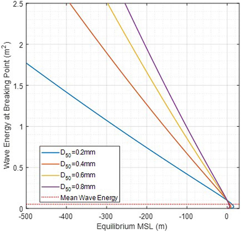
Figure 5. A curve showing the correlation between SL position and energy obtained from Dean’s equilibrium beach profile formula.
Figure 6 shows the wave scenario at the breaking points, and the numerical solutions of Eq. 7 for kr = 0.04, 0.06, and 0.08d−1. The results show that the wave input that causes shoreline change lasts for 2–3 days, but the evolution of the shoreline shows that it is affected for more than 30 days before returning to the original initial shoreline position. For kr = 0.06d−1, it is estimated that approximately 50 days are required for a 95% recovery after maximum shoreline erosion occurs. In this simulation, Hp = 6.0m and ar = 0.007m were used for the peak wave height in deep water and beach response factor, respectively.
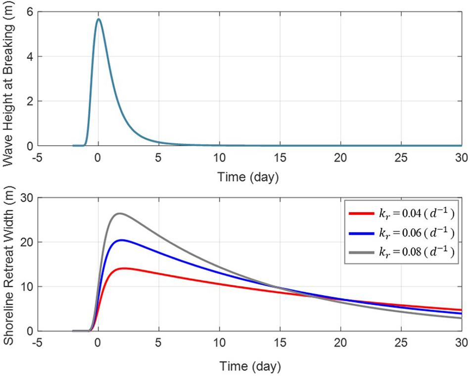
Figure 6. Time evolution of wave scenario and shoreline retreat width for 3 different kr values.
Predicting Peak Erosion Width Using the SWSF Formula
Figure 7 shows the results obtained using Eq. 7 to determine the peak erosion width for peak wave heights of 4.5, 5.5, 6.5, and 7.5 m. The results of the contour line correspond to the proportionality constants of the vulnerability curves. The ranges of the two factors considered were evaluated based on whether they corresponded to a range of values corresponding to a general sand beach. The temporal change in the wave energy at the breaking point given in Eq. 7 was obtained after converting the significant wave height and peak wave period given by the scenario functions into the wave height at the breaking point.
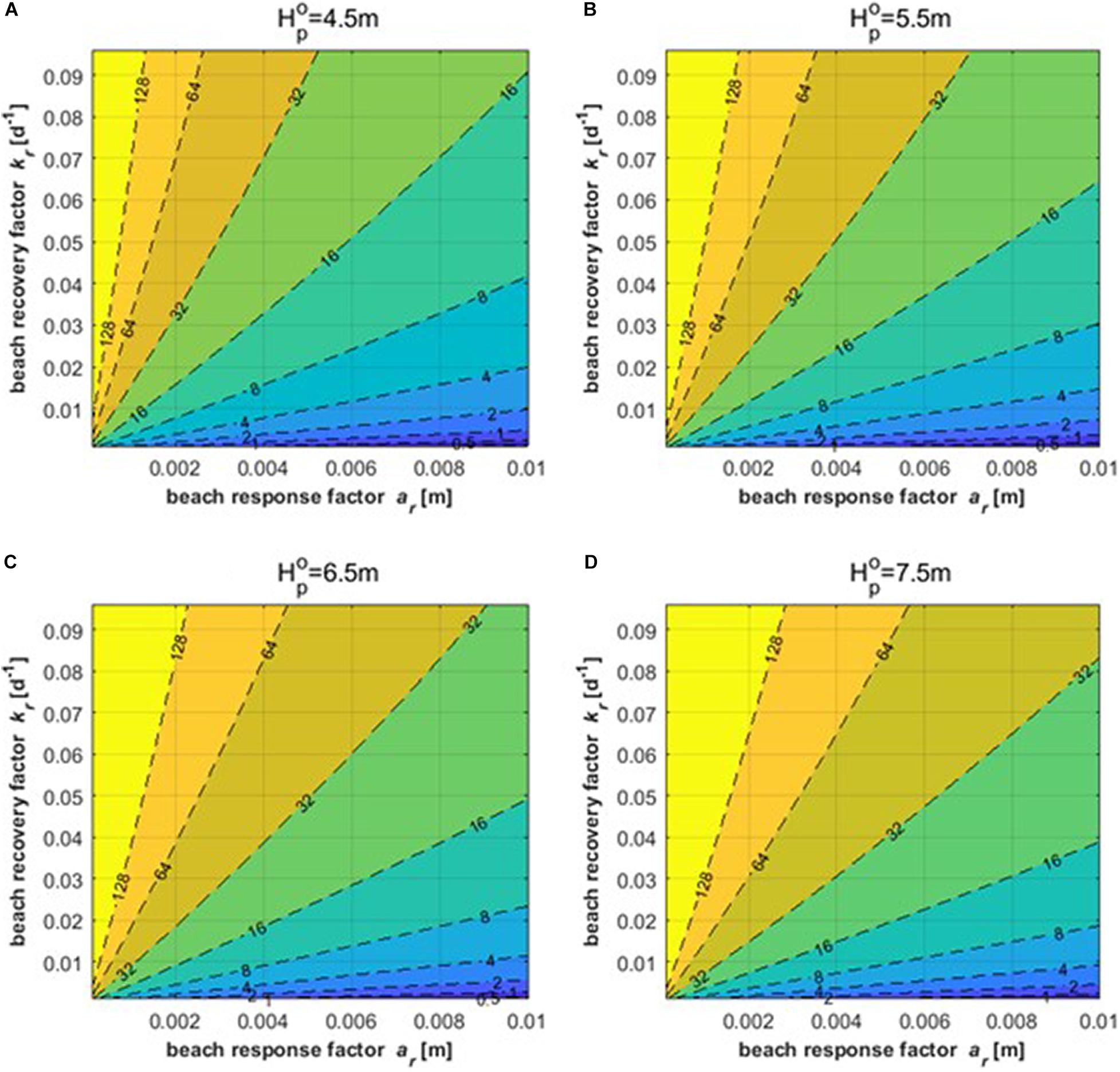
Figure 7. Results of peak SL retreat width according to beach response factor ar(m) and beach recovery factor kr(d−1) for (A) = 4.5m, (B) , (C) , and (D) .
Based on the ODE in Eq. 7, because dy/dt becomes zero at the time of peak SL retreat, when the elapsed time from the peak wave height passing to the peak erosion retreat is τ, Eb(τ)/ar indicates the ypeak. Therefore, ypeak given as a function of τ is:
Figure 8 shows the results of the τ analysis for . As shown by Eq. 13, τ is a function of only kr, regardless of ar.
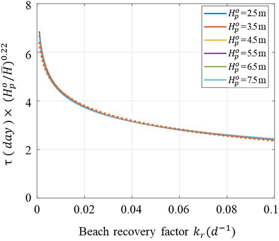
Figure 8. Elapsed time τ from peak wave height to peak erosion width w.r.t the beach recovery factor kr.
where is the peak wave height in deep water, and have the same unit (m), and kr has a unit of d−1.
Figure 9 shows a comparison of the BVC obtained from the model results using Eq. 7 and that obtained from the approximate results using Eq. 12 for the three different values of ar and kr. Compared with each other, they exhibit satisfactory results.
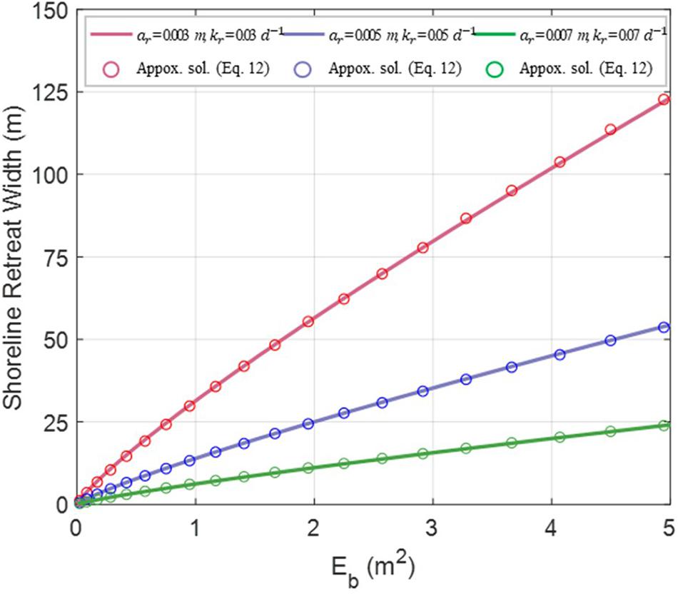
Figure 9. Comparison between model results (Eq. 7) and approximate solutions (Eq. 12) for 3 different points of ar and kr.
Beach Vulnerability Curve for Maengbang Beach
In Section “Derivation of Beach Vulnerability Curve by the Shoreline Response Model,” it was confirmed that the peak erosion width and peak wave energy at the breaking point had a linear correlation without substantial error. The changes in the proportional constant of erosion vulnerability based on ar and kr were calculated using the numerical model results. Therefore, if ar and kr can be determined, based on the sand properties of the beach, we can obtain the erosion vulnerability of the beach. In this section, we demonstrate the validity of this result by comparing it with the vulnerability curves obtained from analysis of the shoreline survey data observed for approximately 9 years at Maengbang Beach in Korea and the NOAA wave data near Maengbang Beach.
Shoreline Survey at Maengbang Beach
Maengbang Beach is one of the target sites for the erosion status survey of Gangwon-do. This sandy beach, with a total length of 4.6 km, stretches to the southeast, and its main incident waves originate from the northeast. Since 2010, GPS shoreline surveys have been conducted at the site four times a year. Beach profile measurements up to a depth of 15 m, sufficiently deeper than the closure depth, were obtained twice a year at 150 m intervals, and the median particle size survey was conducted in the swash zone. The beach profile was measured by potable GNSS on foot from the survey reference point to a water depth of 1.5 m and from 1.5 m to 15 m water depth was surveyed using a bathymetry survey boat equipped with an echo-sounder (single beam). The GNSS model used for shoreline surveying is GX1230 with an accuracy of H: 3 mm + 0.5 ppm. The echo-sounder used for the bathymetric survey is a single beam, the model name is AquaRoller 200S, and the measurement range is 5 ∼ 200 m. These datasets were utilized as basic data to evaluate the coastal erosion grades (A, B, C, and D). In the event of the erosion of the coast, the datasets serve as basic data for cause analysis.
Figure 10 shows the 13 reference points for the survey conducted at Maengbang Beach, which was divided into four survey zones, wherein the mean shoreline and erosion control line (erosion limit for 30 years) were obtained according to the statistical characteristics of the shoreline data. These two shorelines were used for (1) evaluating the management status of Korean coastal regions in terms of conservation and disaster prevention, and (2) evaluating whether the layout design of soft and hard engineering structures of the coastal improvement projects implemented to reduce coastal erosion are achieving the management target lines (mean target shoreline and erosion prevention line).
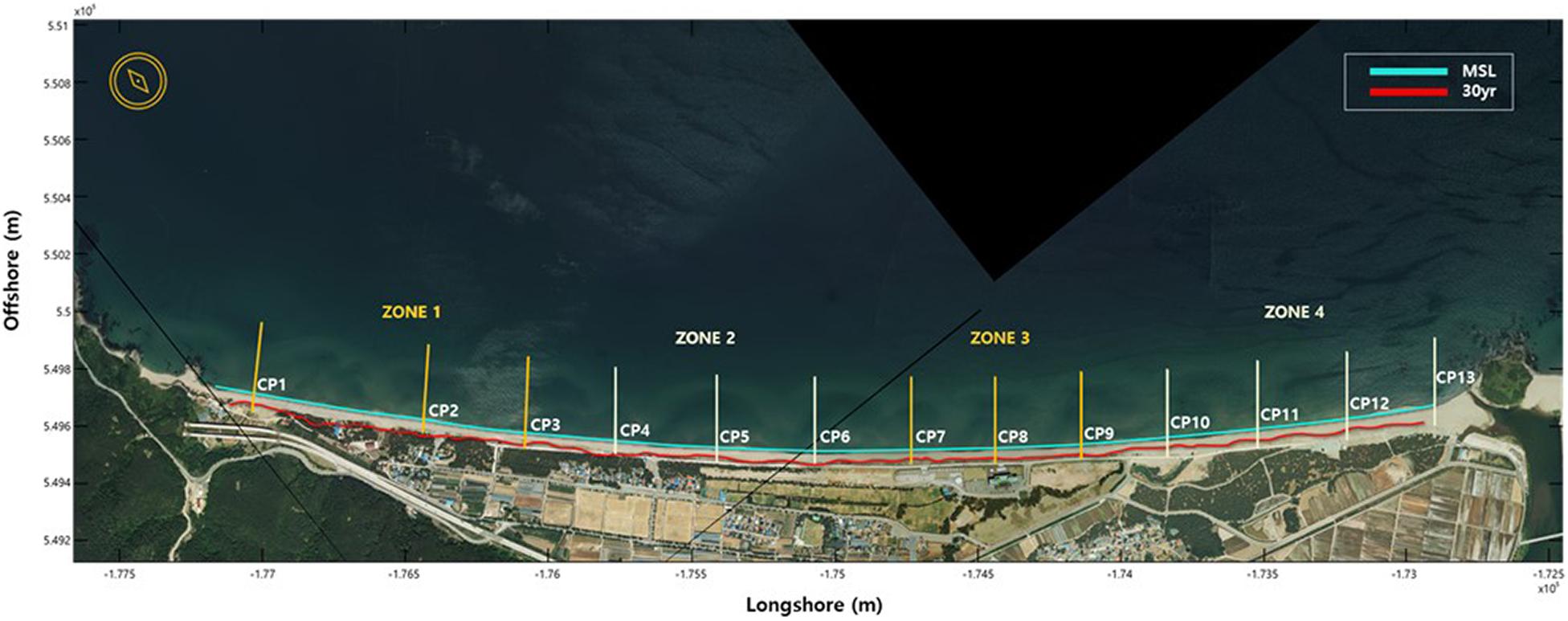
Figure 10. Reference points for median grain size survey, mean shoreline and 30-year erosion control line.
The average D50 obtained for each zone and the corresponding beach scale factor and beach response factor are listed in Supplementary Table 1. Although the average sand particle diameter of Zone 4 was relatively small, the average particle diameter of the entire target beach was 0.656 mm. On the eastern coast of Korea, the net littoral drift flows from the north to the south according to the analysis of long-term wave data and the angle of the coastline (Kim et al., 2001). Owing to this littoral drift environment, the sand on the southern beach may have a finer grain size, but the difference is expected to be small.
Variability Analysis Using Shoreline Survey Data
The shoreline survey of Maengbang Beach, the subject of this study’s beach response analysis, was conducted about five times a year since 2010 as a major observation item in the coastal erosion survey, and was measured at 13 reference points. In the erosion status survey, the shoreline survey is, in principle, conducted once a season. However, in some cases, shoreline surveys were more carried out once or twice a year. Therefore, it resulted in an average of about five shoreline surveys. Figure 11 shows the distribution histograms for each survey zone using 192 shoreline survey datasets collected at 13 reference points (see Figure 10), for which measurements were conducted 47 times from 2010 to 2018. The figure illustrates the probability distribution of the observed shoreline data with reference to the mean values for each zonal reference point. These results were compared to a Gaussian distribution and were found to exhibit high similarity. The statistical frequency analysis of these shoreline observations allows researchers to assess the risk of beach erosion.
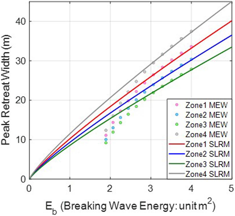
Figure 11. Comparison between MEW and SLRM results.
Zone 1 is located on the northern side of Maengbang Beach, and Zone 4 is located on the southern side of the beach. The results of each zone reasonably follow a normal Gaussian distribution, and according to their statistical characteristics, the monitored erosion width (MEW) can be obtained for each return period (yr). The standard deviation σ for each zone is listed in Supplementary Table 2, as well as the MEW for each zone, which was calculated from the mean value for each return period based on the frequency analysis. These results represent erosion damage by frequency and can therefore be referred to as a risk curve. Conversely, if the extreme wave height analysis result of the NOAA wave data is applied instead of the return frequency, the coastal erosion vulnerability curve (damage curve according to hazards) can be derived.
To verify the normality of the observed shoreline variations, a chi-squared goodness of fit test was performed, confirming that the results follow a normal distribution at the 1% significance level. A qq plot is shown in Supplementary Figure 12. Supplementary Table 2 lists the standard deviation σ of the shoreline survey data for each zone and the MEW for each return period, which was obtained from a variability analysis of the data. The larger the standard deviation, the greater the variability, and thus, the greater the erosion width. Zone 4, which consists of fine sediment, exhibited the highest MEW.
Beach Vulnerability Curve by Shoreline Survey Data
Extreme Wave Height Analysis of Incident Waves
For the extreme wave height analysis, the 40 years long-term wave estimation data provided by NOAA, consisting of 3 h intervals from January 1979 to December 2018, were used. The NOAA deep-sea wave data were converted by applying the shoaling, refraction, and significant wave breaking conditions of Eqs. 4–6 to obtain the wave height at the breaking point. Supplementary Figure 13 shows the results of the extreme wave height analysis conducted using the Gumbel method, and Supplementary Table 3 summarizes the extreme wave height at breaking point HF obtained for each frequency F, which is the reciprocal of the return period. Approximately half of the wave direction components that could not approach the target beach because the wave direction was too wide were excluded from the extreme distribution analysis. The relationship between the extreme wave height (m) and frequency F (yr1) is as follows:
Analysis of Erosion Vulnerability for Maengbang Beach
As mentioned in Section “Variability Analysis Using Shoreline Survey Data,” the MEW for each return period was obtained via an analysis of fluctuations in the monitored shoreline. Therefore, using Eq. 14 to obtain the extreme wave height for each return period, an beach vulnerability curve showing the erosion width for each wave height could be obtained. Supplementary Table 4 lists the calculated MEW for each zone of Maengbang Beach for each extreme wave height at a breaking point of 4.5 m or higher.
Comparison With Beach Vulnerability Curve From Shoreline Response Model
Figure 11 compares the BVC directly obtained from the extreme breaking wave height and the MEW listed in Supplementary Table 4 with the BVC numerically obtained by applying the SWSF to the SLRM. In the SLRM, the beach response factor ar was obtained using Eq. 11 using the sand particle size data, and the beach recovery factor kr was applied as the value with the best fit, as compared to the MEW data for Eb > 2.72m2. The kr values obtained for zones 1–4 were 0.0698, 0.0624, 0.0552, and 0.0796d−1, respectively. When Hb > 6.6m, at which Eb > 2.72m2, there is a satisfactory trend, but when Hb < 6.6m, the values interpreted from the observations are lower than the model predictions, and unlike the model predictions, they do not converge to zero. Instead, the values exhibit a convergence to Eb = 1.73m2, corresponding to the 1-year return period. When the SWSF is shorter than the 1-year return period, the selection of a curve along the maximum coverage line as the scenario model may lead to discrepancies, as shown in Supplementary Figures 9A, 10A.
Zones 1 and 4, which are located at the ends of the beach, show slightly larger kr values than zones 2 and 3. It is presumed that fitting with a larger kr value is probably because of the greater variability at the beach ends, mainly because of the influence of seasonal littoral sedimentation. While kr can be determined from the particle size of the sand, estimating its value is difficult and requires additional research with on-site monitoring. Note that this study is limited to analyzing beach vulnerability in the state where ar and kr are estimated.
As shown in Figure 11, zones 1 and 4, unlike the zones located in the center of the beach, had relatively high kr values compared to the sand grain size, which may be related to the occurrence of littoral drift due to the incidence of oblique waves at the beach ends. On this basis, considering the loss of suspended sediment due to littoral drift, Eq. 7 is modified as follows:
where ε corresponds to the loss rate of suspended sediment caused by the occurrence of littoral drift. If ε is greater than 1, it is considered that suspended particles are introduced from the outside, and when ε is less than 1, it is considered that particles are discharged to the outside. Figure 12 shows how the erosion width varies with ε. In particular, when ε = 0.2 is applied to zones 1 and 4, a reasonable kr is obtained, as compared with that in the surrounding zones. The kr values obtained for zones 1–4 were 0.0628, 0.0624, 0.0522, and 0.0698 d−1, respectively.
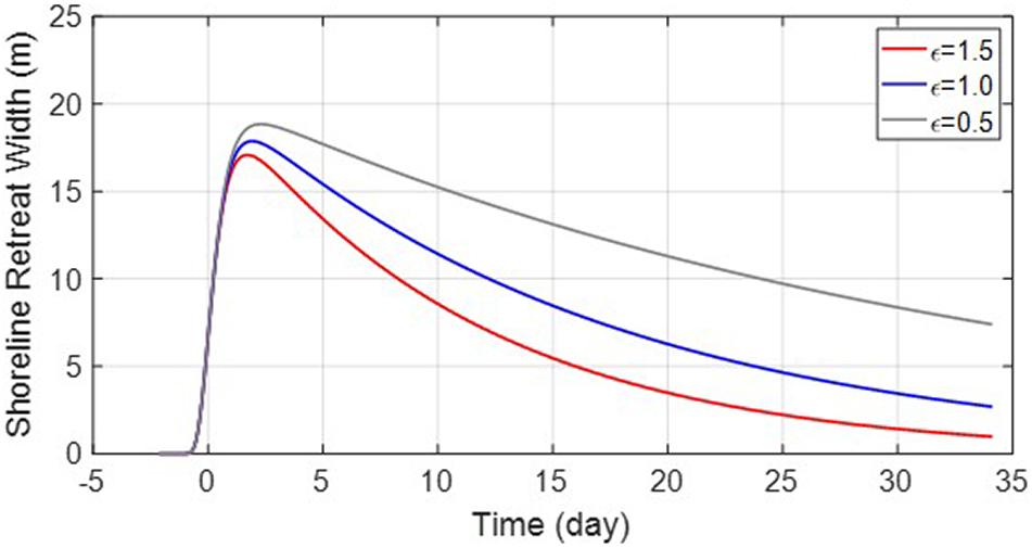
Figure 12. SLRM result according to ε value ( m and ar = 0.008 m).
Discussion
In this study, the SWSF and SLRM were applied to determine the BVC using only cross-shore beach sedimentation based on the values of the beach response factor ar and beach recovery factor kr. The BVC may greatly vary depending on the duration of the coast-specific input SWSF, as well as ar and kr. Specifically, even with the same peak wave height, the erosion width may vary according to the SWSF when subjected to a limited duration. Therefore, in this section, we attempt to determine the time constraint characteristics of the BVC that is less than equilibrium owing to the effect of a limited duration, as compared with the extreme BVC, which has an equilibrium erosion width and the duration of the incoming wave is infinite. In general, we attempt to determine the time constraint characteristics of a BVC that is not in equilibrium by comparing it with the extreme BVC. The extreme BVC corresponds to the results obtained from the field experiments of Yates et al. (2009). However, note that the resulting erosion width is too high to be realistic, and the actual occurrence of erosion of this magnitude would be catastrophic.
When the equilibrium state is reached, the beach erosion vulnerability is roughly expressed by the wave energy at breaking point Eb and the beach erosion vulnerability factor fv:
where ESLP is the equilibrium shoreline position and fv is the reciprocal of the beach response factor ar. This equation is based on Eq. 8, which was modified by ignoring , as it was considered to be relatively small under high wave conditions. Overall, as the vulnerability factor increases, more beach erosion occurs, indicating that the beach erosion vulnerability increases. However, the ESLP refers to a virtual erosion state formed by consistant waves incoming with an infinite duration.
Unlike the ESLP, the duration-limited shoreline position (DSLP), which is affected by duration and has a smaller erosion width, can be expressed as follows:
Therefore, the ratio of the erosion width actually generated by the SWSF compared to the equilibrium erosion width can be defined as the shoreline position ratio μ, as follows:
Supplementary Table 5 lists the calculated τ according to kr and , revealing an elapsed time of approximately 1.5–3 days. Supplementary Table 6 lists the changes in the μ value defined by Eq. 18. These results are valid for the wave conditions at the Maengbang coast. Unlike the ESLP, which is the result of infinite waves of a certain height, the erosion width of the beach that occurs under the actual duration-limited condition, the DSLP, shows a much smaller erosion width, exhibiting values of only approximately μ=0.02−0.11. This is because of the characteristics of the real-world incident storm wave scenario, wherein wave energy is not continuously applied at a constant value but increases and then decreases, not allowing an equilibrium state to be reached.
Figure 13 shows has the effect of spreading SWSF laterally. Overall, as increased, the influence of the duration increased. Although , which is defined as the mean wave height, is unlikely to be greater than 2 m, we assessed the effect of large values to observe the effect of duration. Figure 14A shows that μ becomes larger owing to the effect of longer duration, at constant values of ar and kr. Because μ tends to decrease as wave height increases, / was applied to eliminate this change and obtain a result that barely changes not only with the wave height but also the , as shown in Figure 14B. In addition, considering the change in kr, we obtained the following equation:
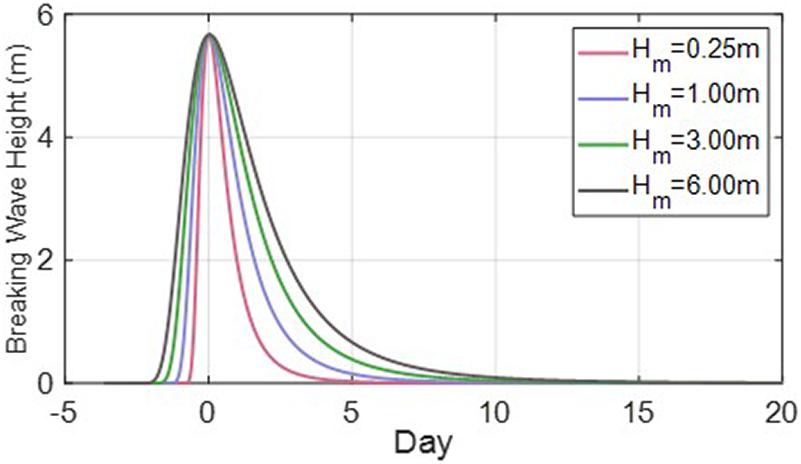
Figure 13. Temporal variation of breaking wave height according to ( and ar = 0.007m and kr = 0.08d−1).
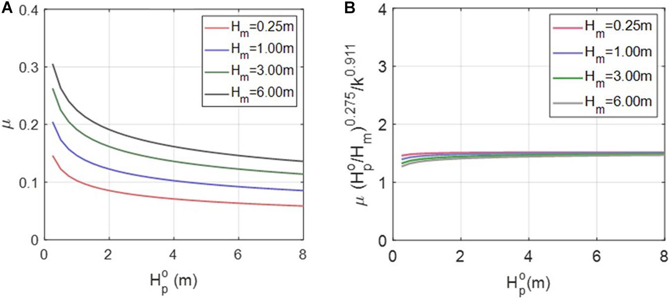
Figure 14. Variation of μ w.r.t ; (A) before scaling with kr = 0.08d−1 and (B) after scaling.
where ar and kr have units of m and d−1, respectively, and the three coefficients α1, α2, and α3 have values of 1.5, −0.275, and 0.911, respectively. By inserting Eq. 19 into Eq. 17, we obtain the following equation, which is useful for the practical application of the DSLP:
Thus, the peak erosion width can be conveniently estimated by using Eq. 20 if the incident peak wave information and characteristic coefficients of the beach responses ar and kr are determined. This gives an idea of how wide the buffer zone should be to avoid the damage to the hinterland for the return period of interest. However, this result ignores the effect of longshore sediment transport and only considers the cross-shore sediment transport process.
We examined whether Eq. 20 provides a satisfactory solution, as compared with the SLRM result. Figure 15 shows the results of the comparison under the same conditions as in Figure 9, revealing fairly agreeable results.
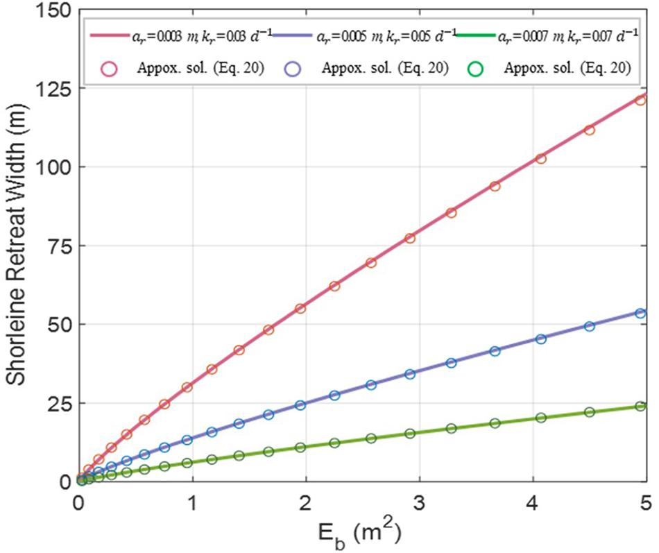
Figure 15. Comparison between model results (Eq. 7) and approximate solutions (Eq. 20) for 3 different points of ar and kr.
The reliability of the BVC (Eq. 20) obtained from the shoreline response model was reviewed by comparing the results obtained from the SLRM by applying SWSF with the results obtained from the statistical analysis of periodic shoreline survey data. All of the 47 shoreline survey data taken in the target area are shown in Supplementary Figure 14, and the average by statistical analysis and the erosion width by return period are plotted thereon. The applicability of the BVC proposed by Eq. 20 was verified and it was confirmed that it showed satisfactory reliability. Supplementary Figure 15 shows the results obtained from BVC among the results shown on the three dimensional LiDAR image. The beach recovery factor kr is the result of considering the effects of littoral drift as described in Section “Comparision with BVC from SLRM”.
Conclusion
Vulnerability is measured as the degree of damage to hazard intensity. In this study, therefore, the storm wave incident scenario to the target beach expressed in terms of the peak wave height, which is the hazard intensity, was established and the scenarios were applied to the SLRM, and the vulnerability curve was extracted by correlating the result of the erosion width, which is the degree of damage. This methodology can be applied to beaches where there are few tidal ranges. Although it may be slightly affected by other factors, such as berm height and initial slope, these effects are considered to be insignificant.
The storm wave scenario function (SWSF) obtained by analyzing NOAA wave data was used as the input data for the SLRM. The numerical results of the model provided satisfactory results compared with the results of shoreline observations, which were conducted five times a year for 9 years on the eastern coast of Korea. Further, while the model did not provide satisfactory results for wave heights with a return period of approximately 1 year or less, it showed fairly good agreement under high wave conditions, which is more meaningful for vulnerability analyzes.
By analyzing the factors affecting erosion vulnerability via the SLRM, an approximate equation with very good consistency was developed. This equation is given by the peak wave height at deep water and the mean wave height in relation to the SWSF, as well as the beach response factor ar and beach recovery factor kr in relation to the SLRM. However, although it is not very difficult, the needs to be converted to Hb by considering wave shoaling, wave refraction, and wave breaking. This BVC approximation provides an intuitive understanding of the factors that influence beach vulnerability and estimates the length of the beach buffer zone required to prevent erosion damage to hinterland facilities over a specific return period. This is expected to provide essential information for limiting reckless coastal development and mitigating erosion damage.
Herein, the SWSF was determined by analyzing the storm wave scenarios with wave heights of 4.5 m or higher from NOAA wave data, which included long-term wave estimation data over 40 years, at 3 h intervals from January 1979 to December at 38.5°N, 129.0°E near Maengbang Beach. To examine the validity of the BVC obtained from the model results, shoreline surveys were conducted approximately five times a year for 9 years and sand size data were used. In the range of Eb > 2.72 m2, the results of SLRM and statistical analysis of MEW variability show quite similar patterns, so the prediction of the peak erosion width by SLRM combined with SWSF is considered reasonable. The beach recovery factor kr in SLRM was applied as the best fit value compared to the MEW data. The kr value is a physical factor affecting the recovery of the shoreline to its original state, and this value is expected to be related to the grain size of the sand. Future research on this is needed.
Because the tidal wave difference is small along the eastern coast of Korea, the SLRM can be directly applied to the coast. However, in the case of the western coast of Korea and other coastal areas with high tidal variations, the influence of incoming high waves evenly affects the intertidal zone, making it difficult to directly apply the methodology of this study. Therefore, in the future, the SLRM must be improved to assess the erosion vulnerability in coastal areas with high tidal variations, to reflect the effect of tides.
Data Availability Statement
The original contributions presented in the study are included in the article/Supplementary Material, further inquiries can be directed to the corresponding author.
Author Contributions
T-KK: conceptualization, acquisition of data, visualization, and writing – editing. CL: acquisition of data, visualization, and writing – editing. J-LL: conceptualization, supervision, validation, and writing – original draft and review. All authors contributed to the article and approved the submitted version.
Funding
This research was part of the “Practical Technologies for Coastal Erosion Control and Countermeasure” project supported by the Ministry of Oceans and Fisheries, South Korea (Grant No. 20180404).
Conflict of Interest
The authors declare that the research was conducted in the absence of any commercial or financial relationships that could be construed as a potential conflict of interest.
Publisher’s Note
All claims expressed in this article are solely those of the authors and do not necessarily represent those of their affiliated organizations, or those of the publisher, the editors and the reviewers. Any product that may be evaluated in this article, or claim that may be made by its manufacturer, is not guaranteed or endorsed by the publisher.
Supplementary Material
The Supplementary Material for this article can be found online at: https://www.frontiersin.org/articles/10.3389/fmars.2021.759067/full#supplementary-material
Supplementary Figure 1 | Location of Maengbang Beach and NOAA data coordinate.
Supplementary Figure 2 | Tide table (A) and wave rose (B) of Maengbang coast.
Supplementary Figure 3 | Time series data of significant wave height (HS) at Maengbang coast from the NOAA dataset (1979–2018).
Supplementary Figure 4 | Time series data of peak wave period (Tp) at Maengbang coast from the NOAA data (1979–2018).
Supplementary Figure 5 | Temporal change of annual mean wave data from 1979 to 2018: (A) annual mean wave height; (B) annual mean wave period; (C) annual mean wave direction.
Supplementary Figure 6 | Joint probability of wave height (HS) and wave period (TS) at Maengbang coast from the NOAA dataset (1979–2018).
Supplementary Figure 7 | Dimensionless wave height scenario model for Maengbang Beach.
Supplementary Figure 8 | Dimensionless wave period scenario model for Maengbang Beach.
Supplementary Figure 9 | Wave scenario models of wave height for Maengbang Beach; (A) 4.5 m ≤ < 5.5 m, (B) 5.5 m ≤ < 6.5 m, (C) 6.5 m , and (D) comparison with respect to peak wave heights.
Supplementary Figure 10 | Wave scenario models of wave period for Maengbang Beach; (A) 4.5 m ≤ < 5.5 m, (B) 5.5 m ≤ < 6.5 m, (C) 6.5 m ≤ , and (D) comparison with respect to peak wave period.
Supplementary Figure 11 | Probability histogram and 30-yr confidence level per zone at Maengbang Beach obtained from shoreline data; (A) Zone 1, (B) Zone 2, (C) Zone 3, and (D) Zone 4.
Supplementary Figure 12 | Result of Chi-squared goodness of fit test at Maengbang Beach obtained from shoreline data.
Supplementary Figure 13 | Extreme distribution function between the return period (yr) and extreme breaking wave height HF (m) obtained from the NOAA data.
Supplementary Figure 14 | Comparison between the erosion width obtained from BVC and monitored erosion width in the study site (A) 10-year return period, and (B) 30-year return period.
Supplementary Figure 15 | Beach profiles estimated from BVC plotted on the three dimensional LiDAR image.
Supplementary Table 1 | Median grain size D50 beach scale factor A and beach response factor ar for each survey zone at Maengbang Beach.
Supplementary Table 2 | Monitored erosion width (MEW) (negative value; -m unit) with respect to return period.
Supplementary Table 3 | Correlations between the return period and extreme breaking wave height HF.
Supplementary Table 4 | Monitored erosion width (MEW) for 4 zones according to the breaking wave height HF.
Supplementary Table 5 | The τ values for deep water wave heights for 4 different kr values.
Supplementary Table 6 | The μ values for each deep water wave heights for 4 different kr values.
References
Anfuso, G., Postacchini, M., Dluccio, D., and Benassai, G. (2021). Coastal sensitivity/vulnerability characterization and adaptation strategies: a review. J. Mar. Sci. Eng. 9:72. doi: 10.3390/jmse9010072
Ballesteros, C., Jimeńez, J. A., Valdemoro, H. I., and Bosom, E. (2017). Erosion consequences on beach functions along the maresme coast (NW Mediterranean, Spain). Nat. Hazards 90, 173–195. doi: 10.1007/s11069-017-3038-5
Bosom, E., and Jimeńez, J. A. (2011). Probabilistic coastal vulnerability assessment to storms at regional scale – application to CataLan beaches (NW Mediterranean). Nat. Hazards Earth Syst. Sci. 11, 475–484. doi: 10.5194/nhess-11-475-2011
Corbella, S., and Stretch, D. D. (2012). Multivariate return periods of sea storms for coastal erosion risk assessment. Nat. Hazards Earth Syst. Sci. 12, 2699–2708. doi: 10.5194/nhess-12-2699-2012
Davidson, M. A., Splinter, K. D., and Turner, I. L. (2013). A simple equilibrium model for predicting shoreline change. Coast. Eng. 73, 191–202. doi: 10.1016/j.coastaleng.2012.11.002
Dean, R. G. (1977). Equilibrium Beach Profiles: U.S. Atlantic and Gulf Coasts, Technical Report No. 12. Newark, DE: Department of Civil Engineering. University of Delaware.
Deltares (2018a). Delft3D-FLOW User Manual: Simulation of Multidimensional Hydrodynamic Flows and Transport Phenomena Including Sediments. Delft: Deltares.
Deltares (2018b). Delft3D-WAVE User Manual: Simulation of Shortcrested Waves with SWAN. Delft: Deltares.
Han, H. J. (2006). Climate Change Impact Assessment and Development of Adatation Strategies in Korea. Sejong: Korea Envirionmental Institute.
IPCC (1996). Climate Change 1995: The Science of Climate Change, eds J. T. Houghton, L. G. M. Filho, B. A. Callander, N. Harris, A. Kattenberg, and K. Maskell Cambridge: Cambridge University Press.
IPCC (2001). Climate Change 2001: Impacts, Adaptation & Vulnerability, Third Assessment Report, eds J. J. McCarthy, O. F. Canziani, N. A. Leary, D. J. Dokken, and K. S. White Cambridge: Cambridge University Press, 184.
Kim, A., Lee, J. L., and Choi, B. H. (2001). Analysis of wave data and estimation of littoral drifts for the eastern coast of Korea. J. Korean Soc. Coast. Ocean Eng. 13, 18–34.
Kim, T. K., and Lee, J. L. (2018). Analysis of shoreline response due to wave energy incidence using equilibrium beach profile concept. J. Ocean Eng. Technol. 32, 116–122. doi: 10.26748/KSOE.2018.4.32.2.116
Kim, T. K., Jeong, J. H., and Lee, J. L. (2021). Shoreline variation analysis by cross-shore sediment transport resulting from effects of storm waves. J. Coast. Res. 114, 539–543. doi: 10.2112/JCR-SI114-109.1
Kriebel, D. L., and Dean, R. G. (1985). Numerical simulation of time-dependent beach and dune erosion. Coast. Eng. 9, 221–245. doi: 10.1016/0378-3839(85)90009-2
Larson, M., Kraus, N. C., and Byrnes, M. R. (1999). SBEACH: Numerical Model For Simulating Storm-Induced Beach change. Report 2Numerical Formulation and Model Tests. Technical Report. CERC-89(9). Vicksburg, MS: U.S. Army Engineer Waterways Experiment Station, 116.
Lesser, G. R., Roelvink, J. A., van Kester, J. A. T. M., and Stelling, G. S. (2004). Development and validation of a three-dimensional morphological model. Coast. Eng. 51, 883–915. doi: 10.1016/j.coastaleng.2004.07.014
Lim, C., Kim, T. K., and Lee, J. L. (2021). Shoreline response induced by spatial suspension and recovery processes of wave-induced sediments. Geomorphology. (Submitted for review)
Madsen, A. J., and Plant, N. G. (2001). Intertidal beach slope predictions compared to field data. Mar. Geol. 173, 121–139. doi: 10.1016/S0025-3227(00)00168-7
Mendoza, E. T., and Jimeńez, J. A. (2006). Storm-induced beach erosion potential on the catalonian coast. J. Coast. Res. SI48, 81–88.
Miller, J. K., and Dean, R. G. (2004). A simple new shoreline change model. Coast. Eng. 51, 531–556. doi: 10.1016/j.coastaleng.2004.05.006
Ministry of Ocean and Fisheries (2017). Coastal Erosion Monitoring in Korea Report. Sejong: Ministry of Ocean and Fisheries.
Montaño, J., Coco, G., Antolnez, J. A. A., Beuzen, T., Bryan, K. R., Cagigal, L., et al. (2020). Blind testing of shoreline evolution models. Sci. Rep. 10:2137. doi: 10.1038/s41598-020-59018-y
Narra, P., Coelho, C., and Sancho, F. (2019). Multicriteria GIS-based estimation of coastal erosion risk: implementation to Aveiro Sandy Coast, Portugal. Ocean Coast. Manag. 178:104845. doi: 10.1016/j.ocecoaman.2019.104845
Oliveira, A., Jesus, G., Gomes, J. L., Rodrigues, M., Fortunato, A. B., Dias, J. M., et al. (2014). An interactive WebGIS observatory platform for enhanced support of integrated coastal management. J. Coast. Res. 70, 507–512. doi: 10.2112/SI70-086.1
Park, S. M., Park, S. H., Lee, J. L., and Kim, T. K. (2019). Erosion control line (ECL) establishment using coastal erosion width prediction model by high wave height. J. Ocean Eng. Technol. 33, 526–534. doi: 10.26748/KSOE.2019.110
Plant, N. G., Holman, R. A., and Freilich, M. H. (1999). A simple model for interannul sandbar behavior. J. Geophys. Res. 104, 15755–15776. doi: 10.1029/1999JC900112
Roelvink, D., Reniers, A., van Dongeren, A., Van Thiel de Vries, J., McCall, R., and Lescinsky, J. (2009). Modelling strom impacts on beaches, dunes and barrier islands. Coast. Eng. 56, 1133–1152. doi: 10.1016/j.coastaleng.2009.08.006
Sorensen, R. M. (1993). Basic Wave Mechanics : for Coastal and Ocean Engineers. New York, NY: John Wiley.
Swart, D. H. (1974). Offshore Sediment Transport and Equilibrium Beach Profiles. Tech. Rep. Publ. 131. Delft: Delft Hydraulics Lab.
Toimil, A., Losada, I. J., Camus, P., and Díaz-Simal, P. (2017). Managing coastal erosion under climate change at the regional scale. Coast. Eng. 128, 106–122. doi: 10.1016/j.coastaleng.2017.08.004
UKCIP (2003). Climate Adaptation: Risk, Uncertainty, and Decision-Making. UKCIP Technical Report. Oxford: UKCIP.
UNDP (2005). Adaptation Policy Framworks for Climate Change: Developing Strategies, Policies, and Measures. Cambridge, MA: Cambridge University Press.
UNFCCC (2005). Compendium on Methods and Tools to Evaluate Impacts of, and Vulnerability and Adaptation to, Climate Change; Final Draft Report. Boulder, CO: Stratus Consulting Inc.
Wright, L. D., Short, A. D., and Green, M. O. (1985a). Short-term changes in the morphologic states of beaches and surf zones: an empirical model. Mar. Geol. 62, 339–364. doi: 10.1016/0025-3227(85)90123-9
Wright, L. D., May, S. K., Short, A. D., and Green, M. O. (1985b). “Prediction of beach and surf zone morphodynamics: equilibria, rates of change and frequency response,” in Proceedings of the 19th Coastal Engineering Conference, 2150–2164.
Yates, M. L., Guza, R. T., and O’Reilly, W. C. (2009). Equilibrium shoreline response: observations and modeling. J. Geophys. Res. 114:C09014. doi: 10.1029/2009JC005359
Keywords: storm wave, numerical model, beach response factor, beach recovery factor, extreme wave analysis, shoreline survey, NOAA wave data
Citation: Kim TK, Lim C and Lee JL (2021) Vulnerability Analysis of Episodic Beach Erosion by Applying Storm Wave Scenarios to a Shoreline Response Model. Front. Mar. Sci. 8:759067. doi: 10.3389/fmars.2021.759067
Received: 15 August 2021; Accepted: 06 October 2021;
Published: 12 November 2021.
Edited by:
Giandomenico Foti, Mediterranea University of Reggio Calabria, ItalyReviewed by:
Kyu-Han Kim, Catholic Kwandong University, South KoreaNoujas Varangalil, National Centre for Coastal Research, India
Copyright © 2021 Kim, Lim and Lee. This is an open-access article distributed under the terms of the Creative Commons Attribution License (CC BY). The use, distribution or reproduction in other forums is permitted, provided the original author(s) and the copyright owner(s) are credited and that the original publication in this journal is cited, in accordance with accepted academic practice. No use, distribution or reproduction is permitted which does not comply with these terms.
*Correspondence: Jung-Lyul Lee, jllee6359@hanmail.net