Evaluating the Spring-Neap Tidal Effects on Chlorophyll-a Variations Based on the Geostationary Satellite

Tides are the dominant hydrodynamic processes in most continental shelf seas and have been proven to have a significant impact on both marine ecosystem dynamics and biogeochemical cycles. In situ and satellite observations have suggested that the spring-neap tide results in fluctuations of chlorophyll-a concentrations (Chl-a) with a fortnightly period in some shelf waters. However, a large number of missing values and low observation frequency in satellite-observed Chl-a have been recognized as the major obstacle to investigating the regional pattern showing where and to what extent of the effects of spring-neap tide on Chl-a and the seasonal variations in the effects within a relatively large region. Taking Himawari-8 as an example, a simple algorithm appropriate for geostationary satellites was proposed in this study with the purpose of obtaining a tide-related daily climatological Chl-a dataset (TDCD) and to quantitatively estimate the effects of the spring-neap tide on Chl-a variations. Based on the Chl-a time series from TDCD, significant fortnightly signals of Chl-a fluctuations and high contribution together with high explanations of the fortnightly fluctuations for Chl-a variations were found in some specific inshore waters, especially in the East China Sea, Bay of Bengal, South China Sea, and northern Australian waters. The spring-neap tide was found able to induce the spatio-temporal fortnightly fluctuations of Chl-a with an annual amplitude of 12–33% of the mean in these inshore areas. Significant seasonal variations in the fortnightly fluctuation of Chl-a were observed in the temperate continental shelf regions, while levels remained relatively stable in the tropical waters. Further analysis implied that the spatio-temporal fortnightly fluctuations of Chl-a were closely associated with the tidal current differences between the spring and neap tides. Seasonal variations in the tidal current differences were found to be a key driving factor for seasonal fluctuations of the spring-neap tidal effects on Chl-a in the temperate continental shelf regions. This study provides a better understanding of tide-related marine ecosystem dynamics and biogeochemical cycles and is helpful in improving physical–biogeochemical models.

Introduction

The continuous global monitoring capability of satellite remote sensing led to its recognition for use in the studies on variations in chlorophyll-a concentrations (Chl-a) since the end of the last century, and our understanding of marine ecosystem dynamics from intraseasonal to interannual time scales with local, regional, or global perspectives has been advanced continually as a result of using this technology (Martinez et al., 2009; Dutkiewicz et al., 2019; Neil et al., 2019; O’Reilly and Werdell, 2019). However, despite their high spatial–temporal resolution, it is still a great challenge to apply these products to studies concerning biological processes or phytoplankton dynamics at short-time scales due to a large number of missing values resulting from cloud coverage, malfunctions of the sensors, or sun glint (Chen et al., 2019). It is worth noting that those short-time scale processes are crucial in the functioning of the marine ecosystems, as physical–biogeochemical models have indicated that marine primary production will increase approximately threefold if short-time scale hydrodynamic processes are included (Mahadevan and Archer, 2000). Clarifying the effects of short-time scale hydrodynamic processes on Chl-a is thus indispensable for understanding the marine ecosystem dynamics and biogeochemical cycles.

Tides are generally regarded as the dominant hydrodynamics in most continental shelves and have been proven to have a significant impact on marine ecosystem dynamics (Shi et al., 2011, 2013; Eleveld et al., 2014). They are characterized by typical spring-neap tidal cycles, which have been revealed to have a great impact on Chl-a fluctuation by in situ observations (Roden, 1994; Sharples et al., 2007; Van der Hout et al., 2017; Díez-Minguito and de Swart, 2020). Specifically, the Chl-a concentration during the spring tide can reach up to approximately 1.7 times higher than that during the neap tide (Koh et al., 2006). Interestingly, it has also been reported that the growth of many fish species shows a fortnightly variation with the peak occurring just after the spring tide, and the bloom of plankton induced by the spring tide may be one of the most important events that account for these biological phenomena (Rahman and Cowx, 2006; Krumme et al., 2008; Li et al., 2021).

Given the importance of spring-neap tidal cycles on marine ecosystems, some studies have attempted to explore the effects of spring-neap tidal cycles on Chl-a variability using polar-orbiting remote sensing satellites (Shi et al., 2013; Gernez et al., 2017; Yang et al., 2020). Generally, most previous studies have focused only on the spatial and temporal variability of Chl-a during a single spring-neap tidal cycle within relatively small areas (e.g., bays and estuaries) due to the missing values in satellite-observed Chl-a (Shi et al., 2013; Gernez et al., 2017; Yang et al., 2020), while the regional pattern showing where and to what extent of this effect still remains unclear. Meanwhile, both tide and Chl-a usually exhibit well-recognized seasonal variations, and it was little-known that these seasonal variations exerted effects on the Chl-a fluctuation induced by spring-neap tides. The short-time scale information in satellite-observed Chl-a was not well captured by the traditional polar-orbiting satellite due to a large number of missing values together with low observational frequency, which has become the major obstacle to evaluating the effects of spring-neap tidal cycles on Chl-a variations together with the seasonal variation of the effects over a relatively large spatial region.

Himawari-8, a new-generation geostationary satellite that carries the Advanced Himawari Imager (AHI), possesses the capacity for full-disk observations every 10 min (see Figure 1 for the whole observational area). The Chl-a products from Himawari-8 employ the blue (470 nm) green (510 nm) ratio for waters with low Chl-a and the green (510 nm) red (640 nm) bands for high Chl-a waters, and this combined method provides higher accuracy for marine Chl-a observation data (Murakami, 2016). The hourly Chl-a products of Himawari-8 have been applied in several submesoscale-related ecological dynamics studies owing to their capability of observing events with short-term scale, such as vortexes (Hsu et al., 2020), typhoons (Iwasaki, 2020; Liu et al., 2020), and upwelling (Shen et al., 2017). These cases demonstrated the applicability of the Chl-a products from Himawari-8 in studies concerning short-term scale marine dynamic processes. Unlike these studies focusing on the short-term event, a more long-term serial dataset with few missing values is necessary to investigate the effects of spring-neap tidal cycles on Chl-a fluctuation and seasonal variations in the effects, posing a great challenge for the application of the Himawari-8 products on this theme. It is imperative to develop a useful algorithm to quantitatively evaluate the effects of spring-neap tidal cycles on Chl-a fluctuation as well as the seasonal variation of the effects using the Chl-a products derived from Himawari-8.

FIGURE 1

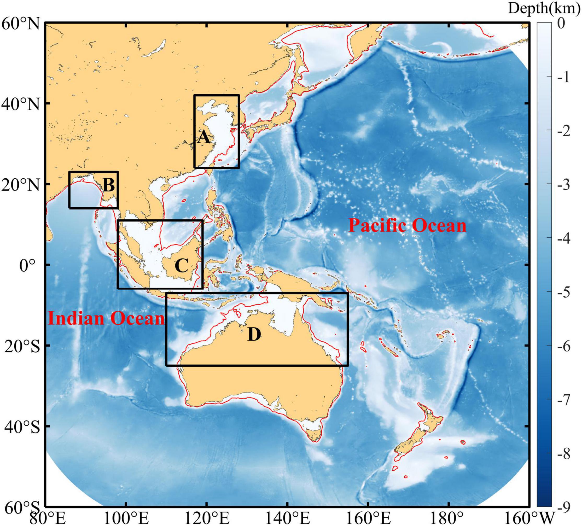
Figure 1. Bathymetry in the whole observational area of Himawari-8. Red lines represent the isobath at 100 m and the Chl-a variations within the four regions in the black boxes (namely, A, B, C, and D) are discussed herein.

Here, a simple method of generating a tide-related daily climatological Chl-a dataset (TDCD) where the Chl-a fluctuations induced by spring-neap tide were highlighted was proposed based on the Himawari-8 Chl-a products by considering the yearly phase differences of the spring-neap tidal cycles. Based on this dataset and statistical methods, the effects of spring-neap tidal cycles on the spatial–temporal variation in Chl-a (especially in four water regions where significant effects of spring-neap tide on Chl-a fluctuation were found) were investigated, including the spatial pattern depicting where and by how much Chl-a is influenced by spring-neap tidal cycles as well as its relationship with tidal currents. The potential mechanisms of the effects and the implications of this study were finally discussed.

Data and Method

Data

Level 3 products of daily Chl-a from July 3, 2015 to December 31, 2019 with 0.05° spatial resolution were used to calculate the TDCD in this study. The data can be downloaded from the P-Tree System, Japan Aerospace Exploration Agency.¹ This product employs a combined algorithm, which was validated by Murakami (2016) as able to derive Chl-a data in both high- and low-concentration waters.

The maximum spring-neap tidal current difference (maximum spring tidal current minus the minimum neap tidal current in each month) was used to investigate the relationship these phenomena have with Chl-a fluctuation. The tidal current data is obtained from the TPXO9 Global Tidal Models, Oregon State University (Egbert and Erofeeva, 2002). This product has a spatial resolution of 1/30° and the assimilation of various altimetric and measured data has led to its application in many tide-related studies (e.g., Yu et al., 2015, 2017).

A Tide-Related Daily Climatological Data Set and Its Algorithm

Here, we propose a simple algorithm appropriate for use with geostationary satellites to capture the fortnightly signals in Chl-a variations, and the multi-year satellite observations of Chl-a are averaged by considering the phase differences of the spring-neap tidal cycles to obtain the TDCD:

(1) The number of days from January 1st to the date of the nearest spring tide (by reference to the moon phases of the new moon from the National Oceanic and Atmospheric Administration) is recorded as di for year i (if the date is nearest to the spring tide in the previous year, di would be negative), and the di for a base year (2019 in this study) is denoted as d1.

(2) The values of di minus d1 can be viewed as the phase difference (dt_i, day) between the spring-neap tidal cycles in year i and that in the base year. The positive dt_i represents the spring-neap tidal cycles in year i occur dt_i days ahead of the base year. All of the dates of Chl-a datasets in year i minus dt_i as the adjusted date based on spring-neap tidal cycles (Figure 2).

(3) The data on the same month and day based on the adjusted date are averaged as the daily climatological value of Chl-a during multi-year satellite observations.

(4) The climatological data contain missing values for approximately 8.66% of the spatio-temporal field, even though data covering four- and half-years are used. A data-interpolating empirical orthogonal function (DINEOF) method is finally used to generate the TDCD without any missing values.

FIGURE 2

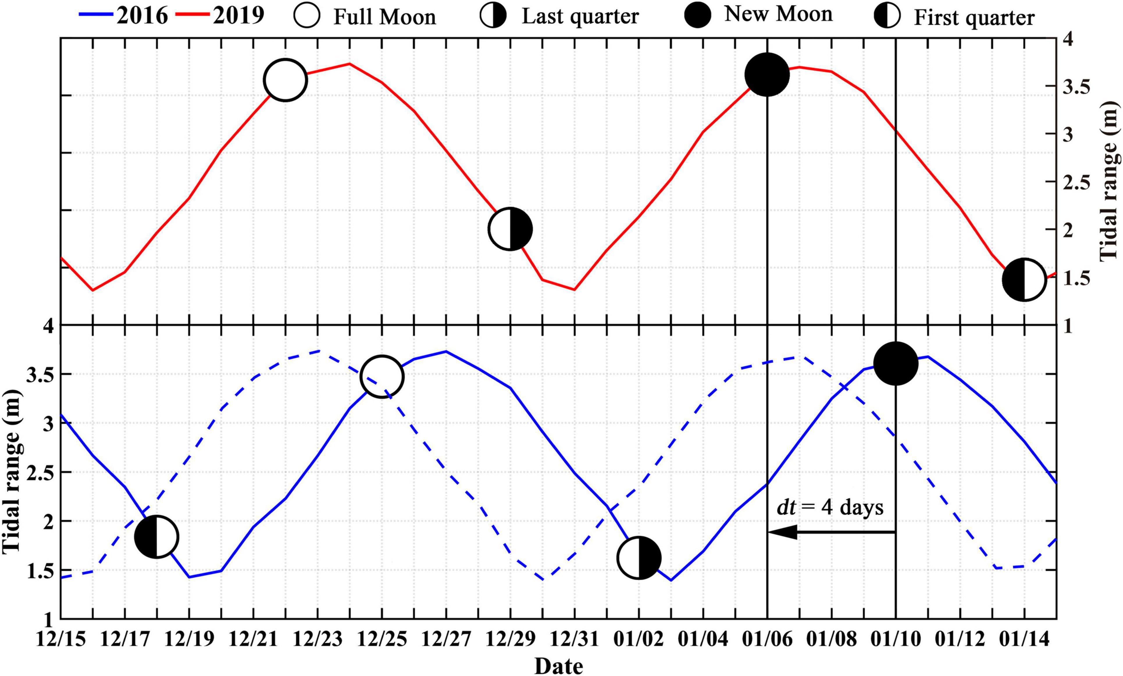
Figure 2. Schematics showing the algorithm used to generate the tide-related daily climatological Chl-a dataset. The blue dashed line stands for the Chl-a time series after the date adjustment based on the phase differences of the spring-neap tidal cycles.

Note: DINEOF is an EOF-based technique developed by Beckers and Rixen (2003) and Alvera-Azcárate et al. (2005), and has been widely used in the reconstruction of marine Chl-a data as it is self-consistent, parameter free, and computationally efficient (Wang and Liu, 2014; Alvera-Azcárate et al., 2015; Hilborn and Costa, 2018). The comparison between DINEOF reconstructed and original Chl-a was shown in Supplementary Material to validate the TDCD. The same merged method was also implemented using the tidal current data to further investigate the effects of the tidal current on Chl-a fluctuations.

Statistical Analyses

Wavelet analysis and significance testing were employed to identify the dominant periodicities in the TDCD using the Morlet wavelet that was the most popular wavelet basis function concerning the researches on ocean science (Torrence and Compo, 1998). Wavelet analysis is a more reasonable method to identify periodic signals than regular spectrum analysis, particularly for the data that changes regularly over time. Morlet wavelet is a Gaussian modulated sine and cosine wave packet, which is able to retrieve the oscillatory behavior of the data effectively, especially in the studies on amplitude and phase changes (Domingues et al., 2005). Wavelet reconstruction was used to recover the Chl-a time series using the periodic signal of the spring-neap tide (13.5–15.5 days) and seasonal trend calculated by low-pass-filtered (90 days) Chl-a time series.

Based on the reconstructed Chl-a time series, the amplitude of Chl-a fluctuation induced by the spring-neap tide can be acquired, and the contribution of the spring-neap tide on Chl-a level can be quantitatively calculated by using the following equation:

$CR=\frac{Ch{l}_a}{Ch{l}_m}\times 100\%(1)$

where, CR represents the contribution rate of Chl-a variations induced by spring-neap tide relative to the averaged Chl-a, Chl_a, and Chl_m denote the amplitude and the mean value of the reconstructed Chl-a of a spring-neap tidal cycle, respectively. Wavelet analysis was implemented with the R package “WaveletComp” in this study (Roesch et al., 2014).

In addition, the proportion of explained variance (PEV, also named R²) from linear regression between the seasonally detrended TDCD and reconstructed Chl-a was acquired to quantify the role of the spring-neap tide in the intra-seasonal variations of the TDCD. Seasonally trend was removed for both TDCD and reconstructed Chl-a to obtain more reliable PEV of the spring-neap tidal cycle as the fortnightly signal was the main focus of this study. PEV has a value of 1 if the fortnightly variation is dominant, while PEV is closer to 0 when the fortnightly variation is negligible.

Considering the changes in mixing and shear force induced by sparing-neap tide, the maximum tidal current differences between spring tide and neap tide were used to explore the mechanism in driving the spatio-temporal variations in the fortnightly fluctuations of Chl-a. The maximum tidal current differences were calculated by the average differences between the maximum tidal current and the minimum tidal current at each neighboring spring-neap tidal cycle.

Results

Fortnightly Variation of Chlorophyll-a and Its Seasonal Changes

Based on the TDCD, wavelet analysis and significance testing were implemented to investigate the periodical variation in Chl-a and its seasonal changes, especially for the four water regions shown in Figure 1. The annual averaged wavelet power clearly indicates that some water regions show prominent fortnightly variation in the time series for Chl-a, such as the Yellow Sea, northern Australian waters, southern Bay of Bengal, and Gulf of Martaban waters (Figure 3). It should be pointed out that although prominent fortnightly variations in Chl-a were mainly found in inshore waters, it is not always the case as there are some regions with prominent fortnightly variations in the time series of Chl-a in the open ocean, like the tropical waters.

FIGURE 3

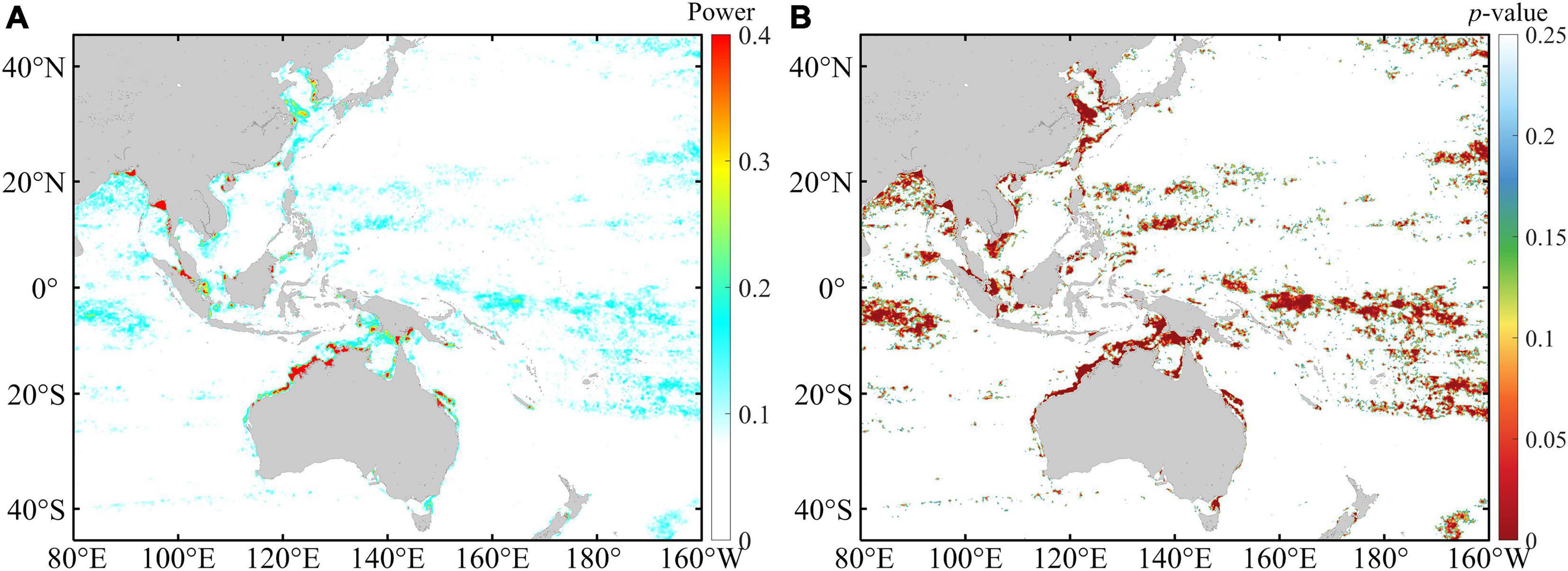
Figure 3. The spatial distribution of (A) the yearly averaged wavelet power maximum over the 14–15 day period and (B) the corresponding level of significance.

Four waters (A, B, C, and D in Figure 1) with prominent fortnightly variation in the Chl-a time series were extracted to investigate the seasonal changes in their periodical fluctuations (only waters that are less than 100 m in depth were included). The selected regions can be regarded as representatives of continental shelf regions in the northern hemisphere, the tropical waters, and the southern hemisphere. It is clear that the averaged wavelet power over the fortnightly period is significant (p < 0.01) in these four regions and the wavelet power is also characterized by obvious seasonal variation (Figure 4). Area A is a representative of the temperate shelf waters in the northern hemisphere, and the time series of Chl-a in this region show strong fortnightly variation in spring, autumn, and winter, while it is significant (p < 0.05) only in April and December. Areas B and D are located in low-latitude shelf waters in the northern and southern hemispheres, respectively. The wavelet power spectrum shows clear seasonality in areas B and D where the significant strong power appears in cold seasons, and such seasonality is even more significant than that in area A. The fortnightly signal appears over the entire year except for April in area C that is located in the tropical ocean; however, it is only significant (p < 0.05) in winter.

FIGURE 4

Figure 4. Wavelet power spectrum and significance level for Chl-a in four typical areas (A–D). The white and black lines represent a significance level of 0.05 and the power ridge, respectively. The significant level of the power spectrum circled by white lines is less than 0.05, and power ridge indicates the local maximization of power spectrum. Black and red dots in the right panels denote the significance level of 0.05 and 0.01 for average wavelet power.

The Contribution Rate of Spring-Neap Tidal Effects on Chlorophyll-a Bloom

Wavelet reconstruction was conducted to reconstruct the 1-year time series using only the spring-neap tide period, and PEV was used to assess the role of spring-neap tide variation in the intra-seasonal fluctuation of the TDCD. Figure 5 shows the comparison between the reconstructed Chl-a and the TDCD. Good consistency is observed between the seasonally detrended TDCD and the recovered Chl-a in all four areas, with PEVs of 62.52, 90.24, 61.25, and 69.99% in A, B, C, and D, respectively, indicating that the spring-neap tidal period plays a dominant role in the intraseasonal variation in these four regions. The annual mean CRs that quantify the contribution of fortnight Chl-a bloom induced by spring-neap tide on Chl-a level were calculated based on the reconstructed time series (Figure 6A). The spatial distribution of the mean CR is slightly different from the annual averaged wavelet power distribution (Figure 3A) as there are significant signals of the spring-neap tidal cycles in some tropical areas that present a lower mean CR. Generally, the CR in inshore waters is higher than that in open waters, and the maximum CR appears on the inshore waters of areas B and D. Figure 6B shows the PEV distribution, which is also consistent with the averaged wavelet power distribution (Figure 3A). The PEV can reach up to approximately 60–70% in waters with a strong signal of spring-neap tidal cycles, while it is less than 15% in areas with deep water depths.

FIGURE 5

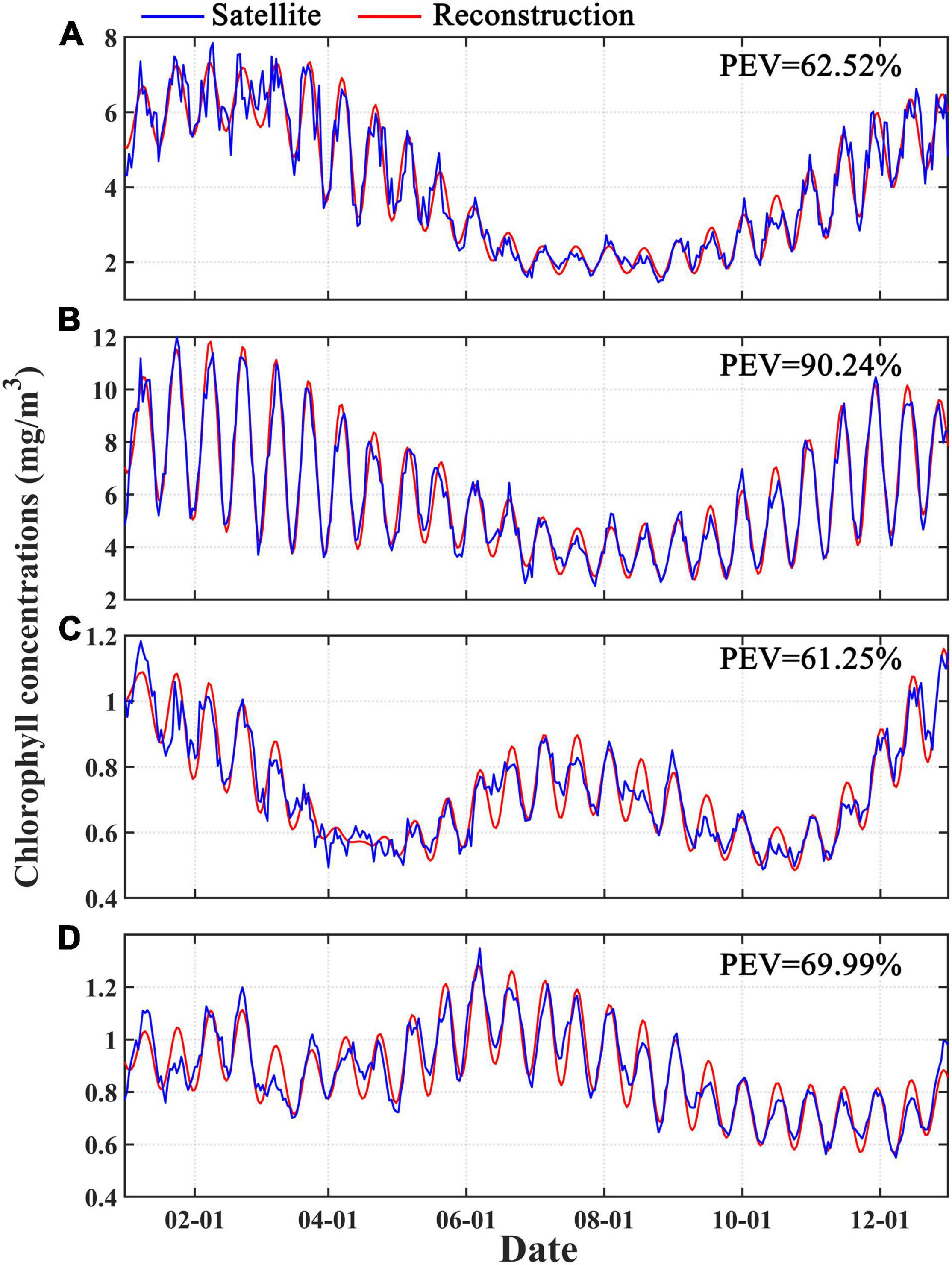
Figure 5. One-year satellite-merged and reconstructed Chl-a derived by wavelet reconstruction for the spring-neap tide cycles in four typical areas (A–D). PEV represents the proportion of explained variance.

FIGURE 6

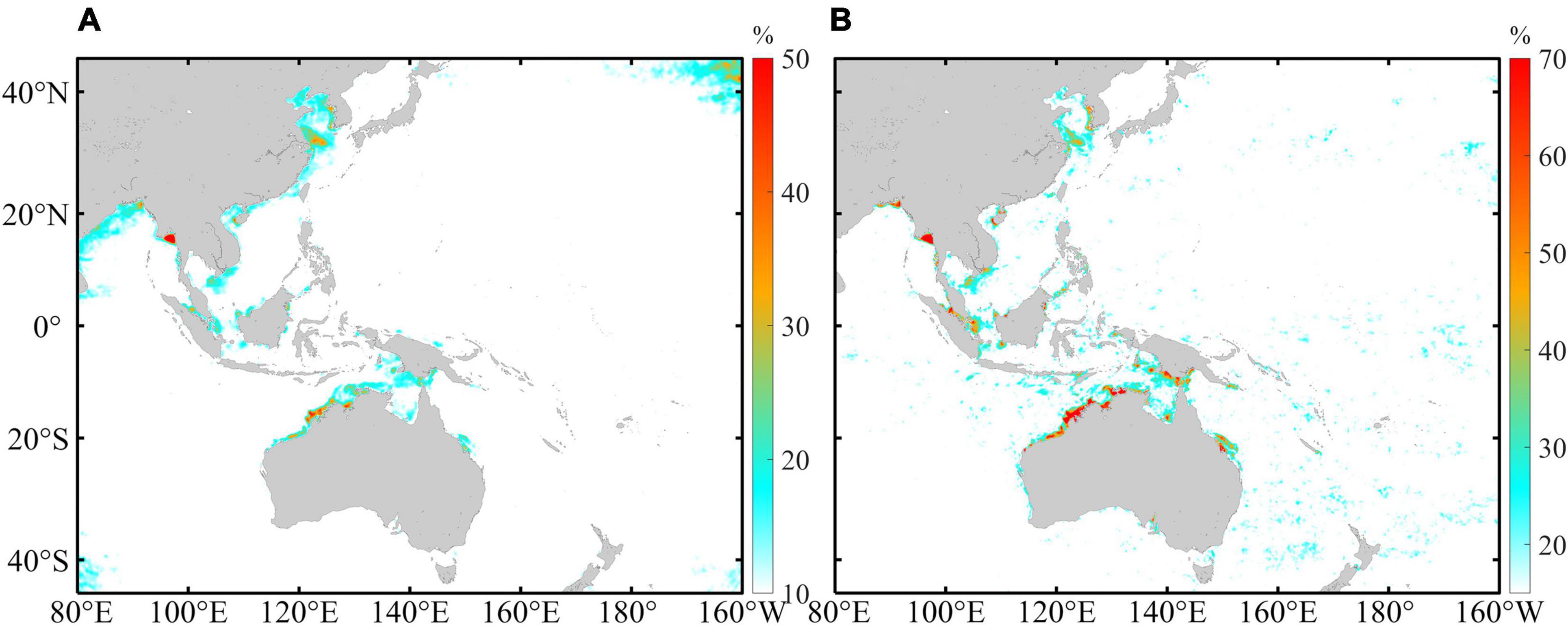
Figure 6. The spatial distribution of (A) yearly average CR representing the contribution of fortnight Chl-a bloom induced by spring-neap tide on Chl-a level and (B) the proportion of intraseasonal variation in Chl-a explained by the spring-neap tidal cycles.

The monthly CRs in the four areas were calculated to evaluate the seasonal variation in the contribution of fortnight Chl-a bloom induced by spring-neap tide on Chl-a level (Figure 7). The CRs for areas A and B are characterized by large seasonal fluctuations with annual mean values of 21.25 and 33.60%, respectively, while they are relatively stable in areas C and D (at approximately 13%). An approximate change of 20% between high and low CRs is found in area B with high CRs in March and November, and high CRs are also observed in area A during April and November with a change of ∼10% between high and low CRs. These results indicate that the effects of the spring-neap tide on Chl-a may differ seasonally in different waters.

FIGURE 7

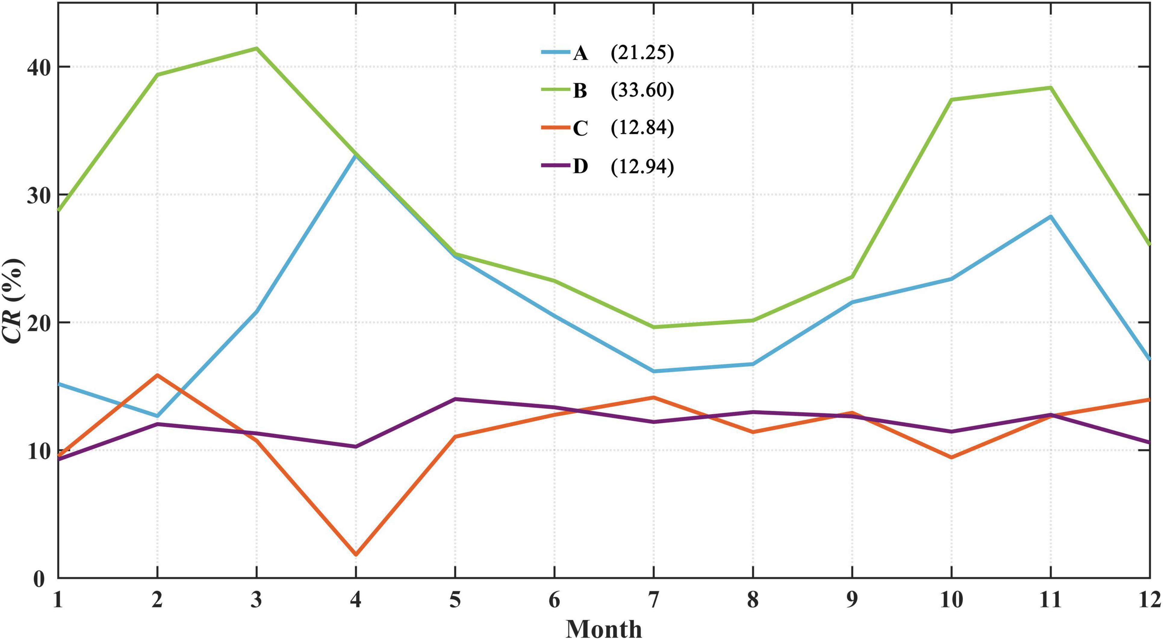
Figure 7. Monthly CRs of spring-neap tidal cycles on Chl-a bloom in four areas. The annual mean CRs are shown in parentheses.

Relationship Between the Tidal Current and Chlorophyll-a Bloom

Here, we employed the maximum tidal current differences between the spring and neap tides to detect the effects of these tides on the CRs. As shown in Figure 8A, large tidal current differences are observed in some inshore waters, while the differences are much smaller in the open waters, which is similar to the spatial distribution of CRs. Taking the whole study area into consideration, the mean CR increases alongside the tidal current differences accompanying by an increase in the standard deviation. The mean CR rises rapidly after the tidal current difference reaches 0.2–0.3 m/s, while it remains relatively stable with decreasing standard deviation when the tidal current difference exceeds 0.5 m/s (Figure 8B). Generally, significant increasing trends in the CR are also observed under higher current differences in the four typical waters (Figure 9). The CR shows a fluctuating upward trend as the current difference increases in area A with the two increasing stages of 0.25–0.4 and 0.6–0.7 m/s, while it maintains a continuously rising trend in area D. Comparatively, the CR increases slowly when the tidal current difference is less than 0.20–0.25 m/s in areas B and C, while it increases rapidly when the tidal current difference exceed 0.20–0.25 m/s.

FIGURE 8

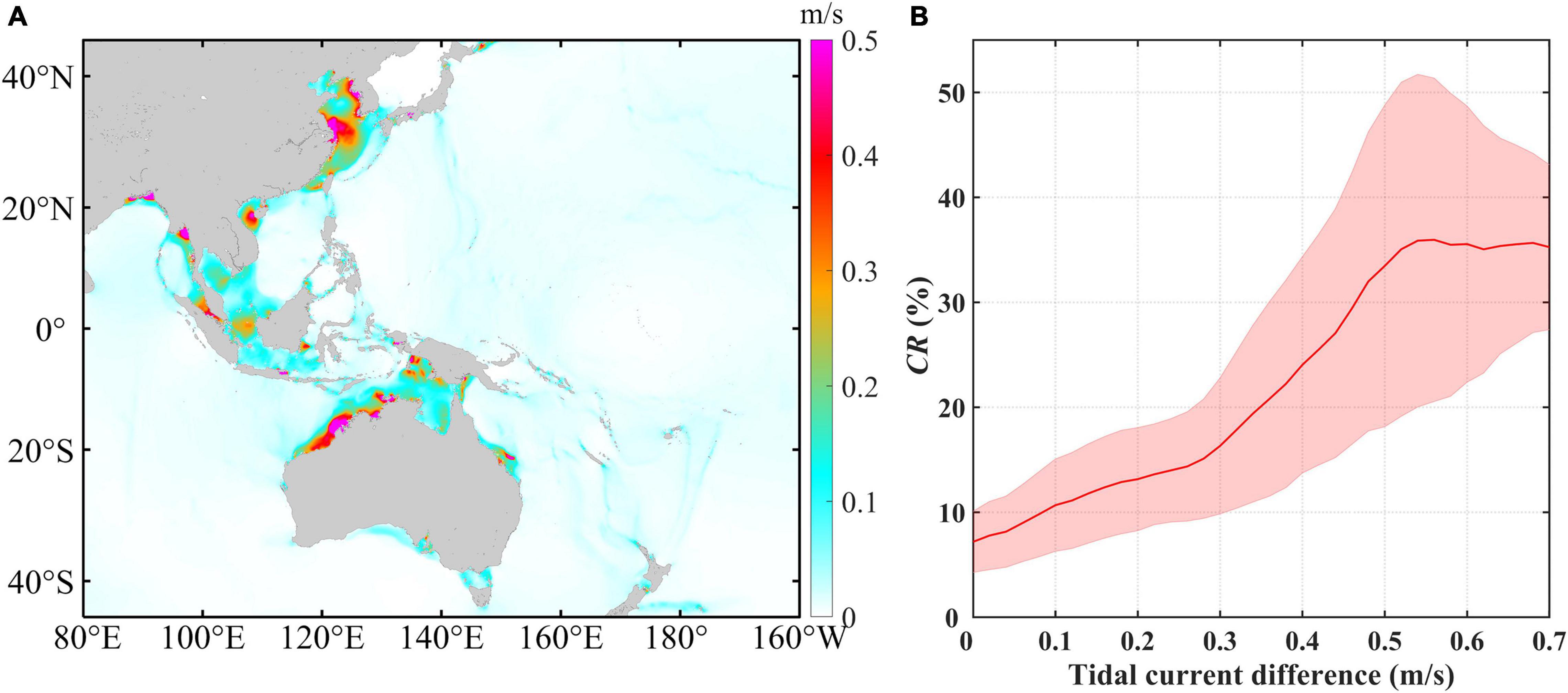
Figure 8. (A) Spatial distribution of the annual averaged spring-neap tidal current difference maximum. (B) Annual averaged spring-neap tidal current difference maximum vs. Chl-a contribution rate (CR) induced by the spring-neap tide. The red curve represents the average and the pink shading indicates the error bar derived from the standard deviation.

FIGURE 9

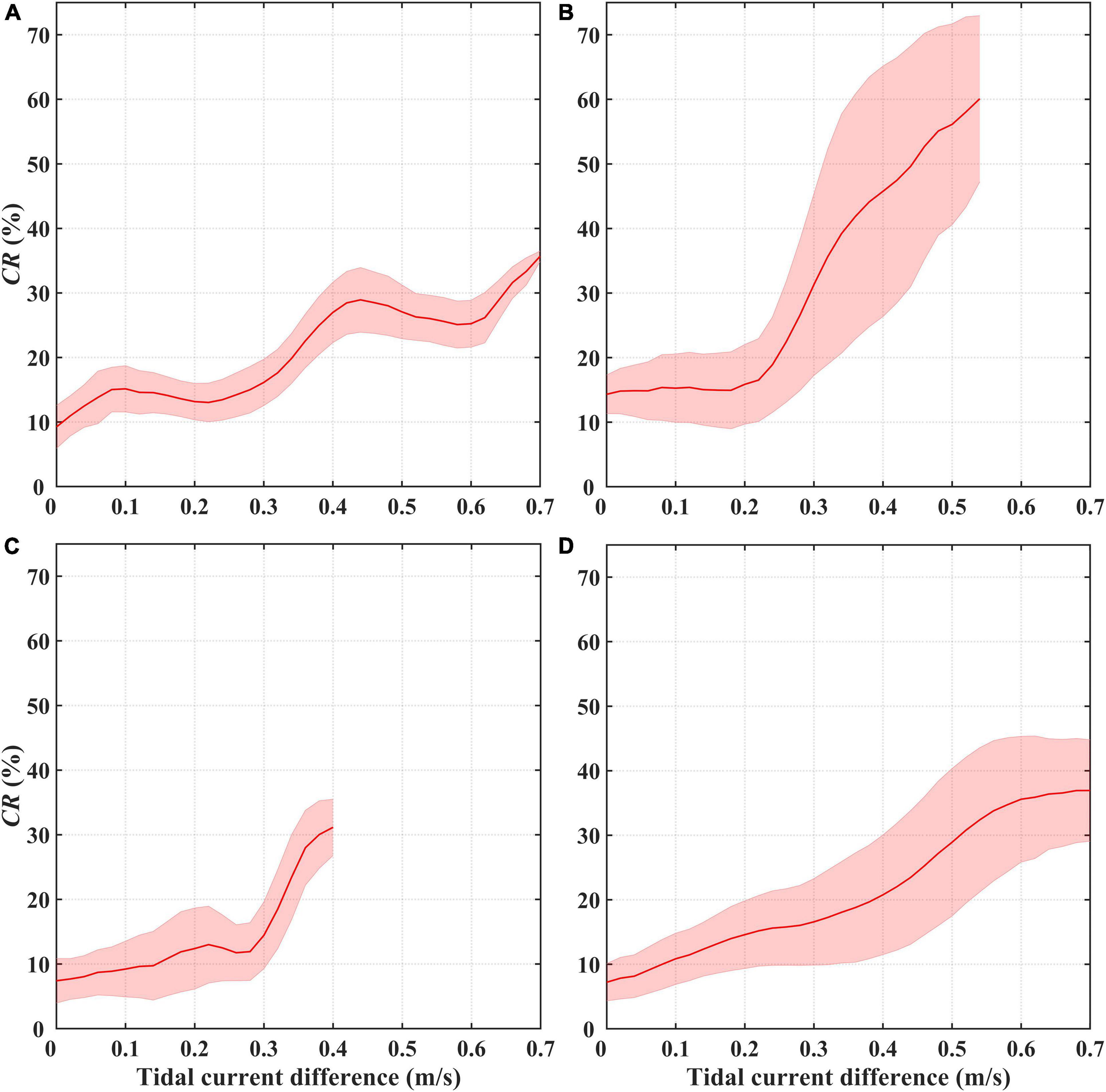
Figure 9. Spring-neap tidal current difference maximum vs. Chl-a contribution rate (CR) induced by the spring-neap tide in areas (A–D). The red curve represents the average and the pink shading indicates the error derived from the standard deviation.

Correlation analysis between the monthly tidal current differences and the CRs variation in areas A, B, C, and D was conducted to further investigate the reason for the different seasonal patterns in the CR variation in different waters. High correlation coefficients are found in areas A, B, and C, but are only significant (p < 0.05) in areas A and C (Figure 10). It should be pointed out that the low and stable CR in areas C and D correspond to lower tidal current differences with low seasonal variance, while the large seasonal fluctuations of the CR in areas A and B are in accordance with the high seasonal variation in the tidal current differences, suggesting that the low seasonal changes in the tidal current differences cause a stable CR. These results indicate that the tidal current difference was a key driving factor for the specific pattern of CR variations in both time and space.

FIGURE 10

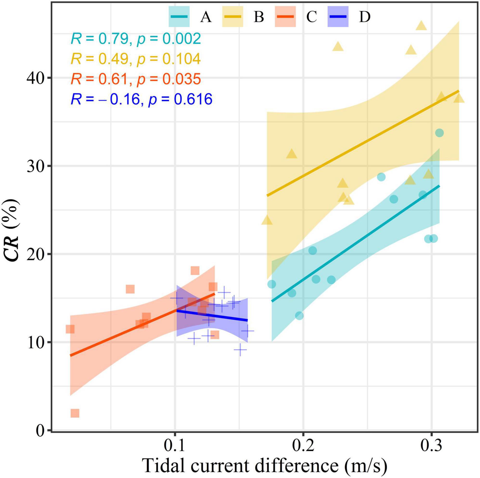
Figure 10. Scatter plots of the spring-neap tidal current difference maximum and Chl-a contribution rate (CR) in areas A, B, C, and D.

Discussion

Potential Mechanism for the Effects of the Spring-Neap Tide on Chlorophyll-a

Previous researches have indicated that some physical processes, such as the enhanced mixing and turbulent dissipation that resulted from the spring tide and led to nutrient renewal, were the key reasons that accounted for the occurrence of the fortnightly fluctuation of Chl-a (Sharples et al., 2007; Su et al., 2015). The observed results showed that the vertical nitrate flux during the spring tide could reach approximately 3.5 mmol m^–2 day^–1, while it was only 1.3 mmol m^–2 day^–1 during the neap tide in the Celtic Sea due to the variation in turbulent dissipation induced by internal spring-neap tide (Sharples et al., 2007). Their numerical model indicated the peak of Chl-a emerged more than 3.5 days behind the maximum of nitrate flux, which was consistent with the phytoplankton carbon turnover rate. Faster algal growth could be found due to remineralized nutrients supply that was related to spring-tidal resuspension events in the German Bight (Su et al., 2015).

Light limitation during spring tide was also an important reason contributing to the fortnightly variations in Chl-a. The numerical model suggested vertical stabilization and better light conditions resulting from low tidal mixing conditions during neap tide brought high total phytoplankton biomass in the Iroise Sea (Cadier et al., 2017). Similarly, continuous field measurement demonstrated that the maximum of Chl-a was found 2–3 days after the neap tide, and weakened vertical mixing was the significant factor for this phenomenon by reducing suspended sediment concentration that regulated light availability (Azhikodan and Yokoyama, 2016).

In addition, several studies have suggested that the resuspended microalgae comprised a large part of the total biomass, and the change in the shear force between the spring and neap tides might result in changes to the resuspended Chl-a (Koh et al., 2006; Blauw et al., 2012; Díez-Minguito and de Swart, 2020), which can be also used to explain the fortnightly variation in Chl-a. It has been reported that suspended microphytobenthos accounted for 92% of the total primary production in the Dollard in the Netherlands (De Jorge and Van Beusekom, 1995), and this proportion can reach up to 71% in the Ariake Sea, Japan (Koh et al., 2006). Interestingly, the mass of resuspended Chl-a usually increased largely at current speeds of >15–20 cm/s, while the resuspension processes were negligible at current speeds under this certain threshold value based on flume and field experiments (Lucas et al., 2000). Microalgae were easily elevated when the current speed was >15–20 cm/s during the early flood tide, and settled when the current speed declined during the ebb period. Meanwhile, better light conditions in the upper water column may also stimulate the primary production of the resuspended microalgae during the spring tide (Lucas et al., 2000; Koh et al., 2006).

Considering the different lag patterns of fortnightly variations in Chl-a behind tidal current in the three possible mechanisms, cross-wavelet power spectrums between daily Chl-a and tidal current time series were further implemented to investigate the potential mechanisms for the effects of the spring-neap tide on Chl-a. Results of the cross-wavelet power spectrums in the four typical areas showed that the significant fortnightly variations in the tidal current were approximately 1.4–2.1 days ahead of the variation in Chl-a (Figure 11), which implied fortnightly variations in Chl-a were in approximate sync with tidal current. The response time of microalgae resuspension on spring-neap tidal cycles was usually characterized by the lower latency than that of the first two possible mechanisms. These results demonstrated that the fluctuation of the resuspended microalgae induced by the change in the shear force during the spring and neap tide was a more dominant cause for the fortnightly fluctuations of Chl-a in our study area, especially in shallow waters.

FIGURE 11

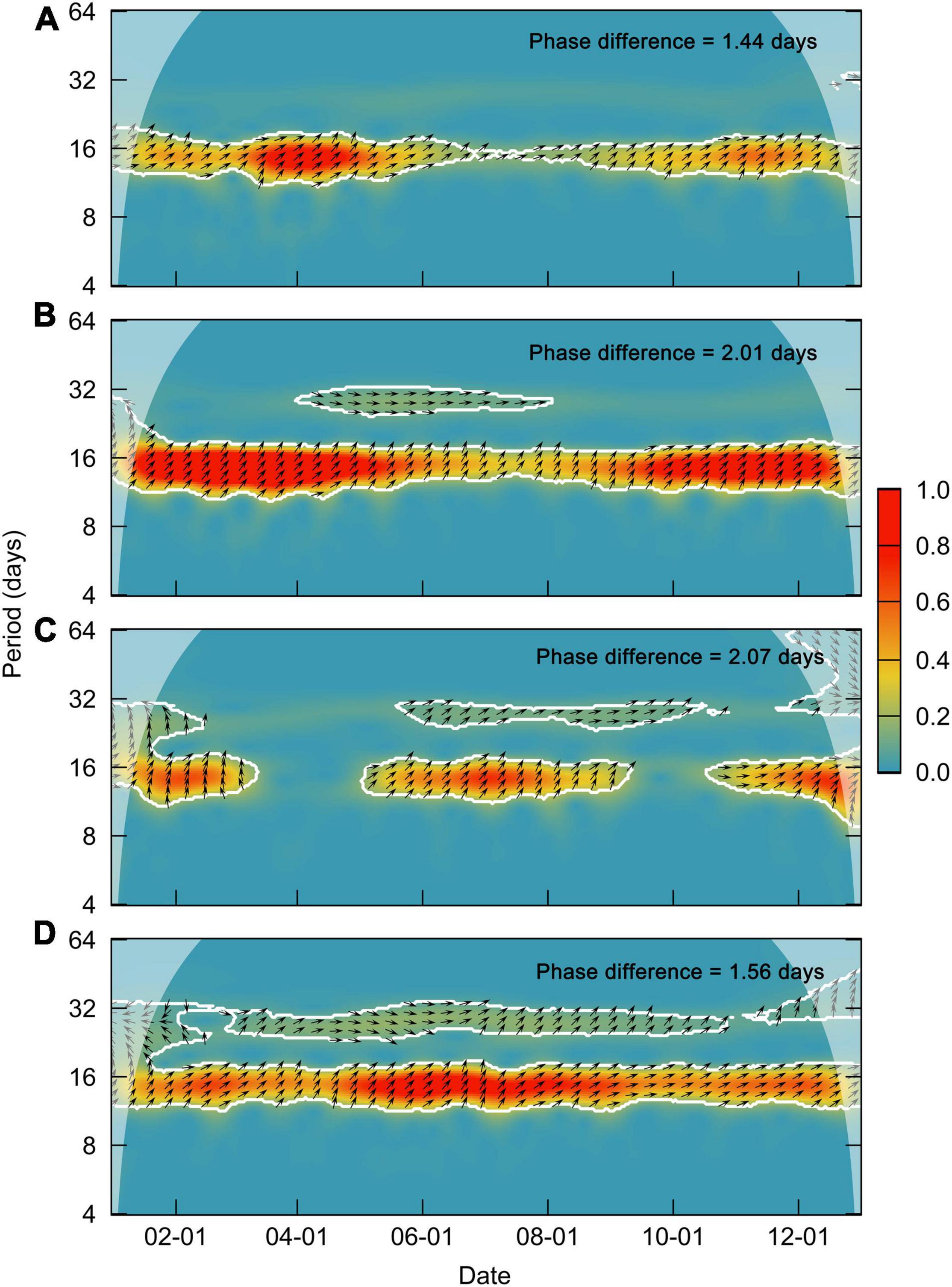
Figure 11. Cross-wavelet power spectrum between daily Chl-a and the tidal current in areas (A–D). The white lines and black arrows represent a significance level of 0.05 and the phase angle between the two time series, respectively.

The significant seasonal variation in CRs was found to be related to the seasonal variation in the spring-neap tidal current differences, especially in areas A and B. The seasonal variations in the spring-neap tidal current differences were induced by the change in the tidal force that results from the seasonal variation in the elliptical orbit of the Earth around the Sun, which caused a seasonal variation in the fortnightly fluctuation of microalgae resuspension. Meanwhile, we also found that the relationships between CRs and the tidal current differences were different in different areas (Figures 9, 10). It should be pointed out that the response of the resuspension process on current velocity was different and depended on the types of sediment (Lucas et al., 2000). Therefore, local biogeochemical processes may also be the key factors that influence the seasonal variation and the spatial pattern of the CRs, and these complicated processes need to be further clarified by the combination of field investigation and physical–biogeochemical models in the future.

Implications and Limitations

It is widely recognized that a large number of missing values in satellite-observed Chl-a data that result from cloud coverage, malfunctioning sensors, or sun glint has become a major obstacle to investigating biological processes and phytoplankton dynamics on short timescales. In this study, we propose a simple algorithm appropriate for use with geostationary satellites to obtain the TDCD. This study is also the first attempt to quantitatively estimate the effects of spring-neap tidal cycles on Chl-a, as well as the seasonal variation in the effects on a relatively large spatial scale, which could provide a better understanding of the ecological dynamic processes modulated by the spring-neap tidal cycle. A feasible approach to optimizing the technologies (e.g., DINEOF, optimal interpolation, etc.) used to fill missing values is also inspired by the TDCD, which is expected to greatly improve the accuracy of the satellite-observed intraseasonal variation in Chl-a that is observed in some tide-dominant regions. Additionally, our findings may also provide implications for improving the parameterization schemes describing physical–biogeochemical models as well as the design of voyage investigations or other monitoring strategies. The proposed algorithm may also be useful for investigating the effects of the spring-neap tidal cycles on other satellite color products (e.g., total suspended matter or colored dissolved organic matter).

However, it should be pointed out that some limitations of the present study are not neglectful before its further application. Although the Level 3 products from Himawari-8 images employs a combined algorithm for derived Chl-a in high and low concentration waters and have been widely used for the researches of short-time scale, its accuracy needs to be further validated especially in inshore waters with high turbidity. The effects of spring-neap tide on Chl-a variations may be overrated due to the uncertainties of derived Chl-a from Himawari-8 in some inshore waters with high turbidity. The algorithm developed by this study will be more valuable in future work to investigate the ecological effect of spring-neap tide based on a validated deriving algorithm of ocean color in different regional areas. Overall, our tide-related algorithm for Chl-a merging benefiting from a validated Chla dataset in different areas from geostationary satellite will comprehensively improve our understanding on the influencing mechanism of tide-related physical-biological processes in the future.

Conclusion

Using a simple algorithm appropriate for geostationary satellites, a tide-related daily climatological data set was obtained, and the effects of the spring-neap tidal cycles on Chl-a variations were quantitatively estimated. Our findings indicated that the spring-neap tide had a strong influence on Chl-a variations in some specific inshore waters, while the effects can be ignored in most of the open seas. The results of wavelet reconstruction suggested that the spring-neap tidal periodic signal can explain more than 63, 90, 61, and 70% of the intraseasonal variations in the climatological Chl-a time series for the four prominent inshore waters investigated. Furthermore, it can be deduced that the spring-neap tide could induce specific spatio-temporal fortnightly variations in Chl-a with an annual amplitude of 12–33% of the mean value in different areas, and the impact was also characterized by obvious seasonal fluctuations in the temperate continental shelf regions, while it remained relatively stable in the tropical waters. The Chl-a fluctuations were closely associated with the maximum current differences between spring and neap tides, as higher current differences may result in stronger fluctuations of Chl-a by enhancing microalgae resuspension. The seasonal variation in tidal current differences was a key driving factor for the seasonal fluctuations observed in the effects of the spring-neap tide on Chl-a in temperate continental shelf regions. The quantitative estimation of the spring-neap tidal effects on Chl-a variations in this study can provide implications for better understanding of marine ecosystem dynamics and biogeochemical cycles, and may also be helpful in the improvement of physical-biogeochemical models as well as the development of methods that can be used to fill missing values in Chl-a dataset that have been obtained by satellites. The findings in present study need to be further improved based on a more reliable Chl-a product from geostationary satellite, especially in inshore waters with high turbidity.

Data Availability Statement

Publicly available datasets were analyzed in this study. This data can be found here: https://www.eorc.jaxa.jp/ptree/index.html; https://www.tpxo.net/.

Author Contributions

QX and HQY conceived and designed the study, performed the data analyses, and wrote the manuscript. QX, HMY, and S-II contributed significantly to the analysis and manuscript preparation. HW, S-II, and CY helped perform the analysis with constructive discussions. All authors contributed to the article and approved the submitted version.

Funding

This work was partially supported by Southern Marine Science and Engineering Guangdong Laboratory (Zhuhai) (No. SML2020SP008), the National Key R&D Program of China (2018YFB1502800), Fundamental Research Funds for the Central Universities (202042004), the National Key R&D Program of China (2018YFB1502800), Fundamental Research Funds for the Central Universities (202042004), the National Natural Science Foundation of China (NSFC) (Nos. 42042018 and 42006016), the Major Science and Technology Innovation Project of Shandong Province (2019JZZY020713), the Natural Science Foundation of Shandong Province (ZR2020QD063), and the key Program of the National Natural Science Foundation of China (91958206).

Conflict of Interest

The authors declare that the research was conducted in the absence of any commercial or financial relationships that could be construed as a potential conflict of interest.

Publisher’s Note

All claims expressed in this article are solely those of the authors and do not necessarily represent those of their affiliated organizations, or those of the publisher, the editors and the reviewers. Any product that may be evaluated in this article, or claim that may be made by its manufacturer, is not guaranteed or endorsed by the publisher.

Acknowledgements

The authors would like to thank the reviewers for their valuable suggestions on the manuscript and also thank Japan Aerospace Exploration Agency for their Chl-a product derived from Himawari-8.

Supplementary Material

The Supplementary Material for this article can be found online at: https://www.frontiersin.org/articles/10.3389/fmars.2021.758538/full#supplementary-material

Footnotes

1. ^ https://www.eorc.jaxa.jp/ptree/index.html

References

Alvera-Azcárate, A., Barth, A., Rixen, M., and Beckers, J. M. (2005). Reconstruction of incomplete oceanographic data sets using empirical orthogonal functions: application to the Adriatic Sea surface temperature. Ocean Modell. 9, 325–346. doi: 10.1016/j.ocemod.2004.08.001

CrossRef Full Text | Google Scholar

Alvera-Azcárate, A., Vanhellemont, Q., Ruddick, K., Barth, A., and Beckers, J. M. (2015). Analysis of high frequency geostationary ocean colour data using DINEOF. Estuar. Coast. Shelf Sci. 159, 28–36. doi: 10.1016/j.ecss.2015.03.026

CrossRef Full Text | Google Scholar

Azhikodan, G., and Yokoyama, K. (2016). Spatio-temporal variability of phytoplankton (Chlorophyll-a) in relation to salinity, suspended sediment concentration, and light intensity in a macrotidal estuary. Cont. Shelf Res. 126, 15–26. doi: 10.1016/j.csr.2016.07.006

CrossRef Full Text | Google Scholar

Beckers, J. M., and Rixen, M. (2003). EOF calculations and data filling from incomplete oceanographic datasets. J. Atmos. Ocean. Technol. 20, 1839–1856.

Google Scholar

Blauw, A. N., Beninca, E., Laane, R. W., Greenwood, N., and Huisman, J. (2012). Dancing with the tides: fluctuations of coastal phytoplankton orchestrated by different oscillatory modes of the tidal cycle. PLoS One 7:e49319. doi: 10.1371/journal.pone.0049319

PubMed Abstract | CrossRef Full Text | Google Scholar

Cadier, M., Gorgues, T., LHelguen, S., Sourisseau, M., and Memery, L. (2017). Tidal cycle control of biogeochemical and ecological properties of a macrotidal ecosystem. Geophys. Res. Lett. 44, 8453–8462. doi: 10.1002/2017GL074173

CrossRef Full Text | Google Scholar

Chen, S., Hu, C., Barnes, B. B., Xie, Y., Lin, G., and Qiu, Z. (2019). Improving ocean color data coverage through machine learning. Remote Sens. Environ. 222, 286–302. doi: 10.1016/j.rse.2018.12.023

CrossRef Full Text | Google Scholar

De Jorge, V. N., and Van Beusekom, J. E. E. (1995). Wind- and tide-induced resuspension of sediment and microphytobenthos from tidal flats in the Ems estuary. Limnol. Oceanogr. 40, 776–778. doi: 10.4319/lo.1995.40.4.0776

CrossRef Full Text | Google Scholar

Díez-Minguito, M., and de Swart, H. E. (2020). Relationships between Chlorophyll-a and suspended sediment concentration in a high-nutrient load estuary: an observational and idealized modeling approach. J. Geophys. Res. Oceans 125:e2019JC015188. doi: 10.1029/2019JC015188

CrossRef Full Text | Google Scholar

Domingues, M. O., Mendes, O. Jr., and da Costa, A. M. (2005). On wavelet techniques in atmospheric sciences. Adv. Space Res. 35, 831–842.

Google Scholar

Dutkiewicz, S., Hickman, A. E., Jahn, O., Henson, S., Beaulieu, C., and Monier, E. (2019). Ocean colour signature of climate change. Nat. Commun. 10:578. doi: 10.1038/s41467-019-08457-x

PubMed Abstract | CrossRef Full Text | Google Scholar

Egbert, G. D., and Erofeeva, S. Y. (2002). Efficient inverse modeling of barotropic ocean tides. J. Atmos. Ocean. Technol. 19, 183–204.

Google Scholar

Eleveld, M. A., Van der Wal, D., and Van Kessel, T. (2014). Estuarine suspended particulate matter concentrations from sun-synchronous satellite remote sensing: tidal and meteorological effects and biases. Remote Sens. Environ. 143, 204–215. doi: 10.1016/j.rse.2013.12.019

CrossRef Full Text | Google Scholar

Gernez, P., Doxaran, D., and Barillé, L. (2017). Shellfish aquaculture from space: potential of Sentinel2 to monitor tide-driven changes in turbidity, chlorophyll concentration and oyster physiological response at the scale of an oyster farm. Front. Mar. Sci. 4:137. doi: 10.3389/fmars.2017.00137

CrossRef Full Text | Google Scholar

Hilborn, A., and Costa, M. (2018). Applications of DINEOF to satellite-derived chlorophyll-a from a productive coastal region. Remote Sens. 10:1449. doi: 10.3390/rs10091449

CrossRef Full Text | Google Scholar

Hsu, P. C., Ho, C. Y., Lee, H. J., Lu, C. Y., and Ho, C. R. (2020). Temporal variation and spatial structure of the Kuroshio-induced submesoscale island vortices observed from GCOM-C and Himawari-8 data. Remote Sens. 12:883. doi: 10.3390/rs12050883

CrossRef Full Text | Google Scholar

Iwasaki, S. (2020). Daily variation of Chlorophyll-A concentration increased by typhoon activity. Remote Sens. 12:1259. doi: 10.3390/rs12081259

CrossRef Full Text | Google Scholar

Koh, C. H., Khim, J. S., Araki, H., Yamanishi, H., Mogi, H., and Koga, K. (2006). Tidal resuspension of microphytobenthic chlorophyll a in a Nanaura mudflat, Saga, Ariake Sea, Japan: flood–ebb and spring–neap variations. Mar. Ecol. Prog. Series 312, 85–100. doi: 10.3354/meps312085

CrossRef Full Text | Google Scholar

Krumme, U., Brenner, M., and Saint-Paul, U. (2008). Spring-neap cycle as a major driver of temporal variations in feeding of intertidal fishes: evidence from the sea catfish Sciades herzbergii (Ariidae) of equatorial west Atlantic mangrove creeks. J. Exp. Mar. Biol. Ecol. 367, 91–99. doi: 10.1016/j.jembe.2008.08.020

CrossRef Full Text | Google Scholar

Li, J., Jiang, F., Wu, R., Zhang, C., Tian, Y., Sun, P., et al. (2021). Tidally induced temporal variations in growth of young-of-the-year Pacific cod in the Yellow Sea. J. Geophy. Res.Oceans 126:e2020JC016696. doi: 10.1029/2020JC016696

CrossRef Full Text | Google Scholar

Liu, S., Li, J., Sun, L., Wang, G., Tang, D., Huang, P., et al. (2020). Basin-wide responses of the South China Sea environment to Super Typhoon Mangkhut (2018). Sci. Total Environ. 731:139093. doi: 10.1016/j.scitotenv.2020.139093

PubMed Abstract | CrossRef Full Text | Google Scholar

Lucas, C. H., Widdows, J., Brinsley, M. D., Salkeld, P. N., and Herman, P. M. (2000). Benthic-pelagic exchange of microalgae at a tidal flat. 1 pigment analysis. Mar. Ecol. Prog. Series 196, 59–73. doi: 10.3354/Meps196059

CrossRef Full Text | Google Scholar

Mahadevan, A., and Archer, D. (2000). Modeling the impact of fronts and mesoscale circulation on the nutrient supply and biogeochemistry of the upper ocean. J. Geophys. Res. Oceans 105, 1209–1225. doi: 10.1029/1999JC900216

CrossRef Full Text | Google Scholar

Martinez, E., Antoine, D., D’Ortenzio, F., and Gentili, B. (2009). Climate-driven basin-scale decadal oscillations of oceanic phytoplankton. Science 326, 1253–1256. doi: 10.1126/science.1177012

PubMed Abstract | CrossRef Full Text | Google Scholar

Murakami, H. (2016). “Ocean color estimation by Himawari-8/AHI,” in Proceedings of the Remote Sensing of the Oceans and Inland Waters: Techniques, Applications, and Challenges, Vol. 9878, (Bellingham, WA: International Society for Optics and Photonics), 987810.

Google Scholar

Neil, C., Spyrakos, E., Hunter, P. D., and Tyler, A. N. (2019). A global approach for chlorophyll-a retrieval across optically complex inland waters based on optical water types. Remote Sens. Environ. 229, 159–178. doi: 10.1016/j.rse.2019.04.027

CrossRef Full Text | Google Scholar

O’Reilly, J. E., and Werdell, P. J. (2019). Chlorophyll algorithms for ocean color sensors-OC4, OC5 & OC6. Remote Sens. Environ. 229, 32–47. doi: 10.1016/j.rse.2019.04.021

PubMed Abstract | CrossRef Full Text | Google Scholar

Rahman, M. J., and Cowx, I. G. (2006). Lunar periodicity in growth increment formation in otoliths of hilsa shad (Tenualosa ilisha, Clupeidae) in Bangladesh waters. Fish. Res. 81, 342–344. doi: 10.1016/j.fishres.2006.06.026

CrossRef Full Text | Google Scholar

Roden, C. M. (1994). Chlorophyll blooms and the spring/neap tidal cycle: observations at two stations on the coast of Connemara, Ireland. Mar. Biol. 118, 209–213. doi: 10.1007/BF00349786

CrossRef Full Text | Google Scholar

Roesch, A., Schmidbauer, H., and Roesch, M. A. (2014). Package ‘WaveletComp’. The Comprehensive R Archive Network2014.

Google Scholar

Sharples, J., Tweddle, J. F., Mattias Green, J. A., Palmer, M. R., Kim, Y. N., Hickman, A. E., et al. (2007). Spring-neap modulation of internal tide mixing and vertical nitrate fluxes at a shelf edge in summer. Limnol. Oceanogr. 52, 1735–1747. doi: 10.2307/4502331

CrossRef Full Text | Google Scholar

Shen, D., Li, X., Pietrafesa, L., and Bao, S. (2017). “Geostationary satellite observations and numerical simulation of typhoon-induced upwelling to the Northeast of Taiwan,” in Proceedings of the 2017 IEEE International Geoscience and Remote Sensing Symposium (IGARSS) (Fort Worth, TX: IEEE), 3552–3555. doi: 10.1109/IGARSS.2017.8127766

CrossRef Full Text | Google Scholar

Shi, W., Wang, M., and Jiang, L. (2011). Spring-neap tidal effects on satellite ocean color observations in the Bohai Sea, Yellow Sea, and East China Sea. J. Geophys. Res. Oceans 116:C12. doi: 10.1029/2011JC007234

CrossRef Full Text | Google Scholar

Shi, W., Wang, M., and Jiang, L. (2013). Tidal effects on ecosystem variability in the Chesapeake Bay from MODIS-Aqua. Remote Sens. Environ. 138, 65–76. doi: 10.1016/j.rse.2013.07.002

CrossRef Full Text | Google Scholar

Su, J., Tian, T., Krasemann, H., Schartau, M., and Wirtz, K. (2015). Response patterns of phytoplankton growth to variations in resuspension in the German Bight revealed by daily MERIS data in 2003 and 2004. Oceanologia 57, 328–341. doi: 10.1016/j.oceano.2015.06.001

CrossRef Full Text | Google Scholar

Torrence, C., and Compo, G. P. (1998). A practical guide to wavelet analysis. Bull. Am. Meteorol. Soc. 79, 61–78.

Google Scholar

Van der Hout, C. M., Witbaard, R., Bergman, M. J. N., Duineveld, G. C. A., Rozemeijer, M. J. C., and Gerkema, T. (2017). The dynamics of suspended particulate matter (SPM) and chlorophyll-a from intratidal to annual time scales in a coastal turbidity maximum. J. Sea Res. 127, 105–118. doi: 10.1016/j.seares.2017.04.011

CrossRef Full Text | Google Scholar

Wang, Y., and Liu, D. (2014). Reconstruction of satellite chlorophyll-a data using a modified DINEOF method: a case study in the Bohai and Yellow seas, China. Int. J. Remote Sens. 35, 204–217. doi: 10.1080/01431161.2013.866290

CrossRef Full Text | Google Scholar

Yang, M., Goes, J. I., Tian, H., Maúre, E. D. R., and Ishizaka, J. (2020). Effects of spring–neap tidal cycle on spatial and temporal variability of satellite Chlorophyll-A in a Macrotidal Embayment, Ariake Sea, Japan. Remote Sens. 12:1859. doi: 10.3390/rs12111859

CrossRef Full Text | Google Scholar

Yu, H., Yu, H., Ding, Y., Wang, L., and Kuang, L. (2015). On M2 tidal amplitude enhancement in the Taiwan Strait and its asymmetry in the cross-strait direction. Cont. Shelf Res. 109, 198–209. doi: 10.1016/j.csr.2015.09.005

CrossRef Full Text | Google Scholar

Yu, H., Yu, H., Wang, L., Kuang, L., Wang, H., Ding, Y., et al. (2017). Tidal propagation and dissipation in the Taiwan Strait. Cont. Shelf Res. 136, 57–73. doi: 10.1016/j.csr.2016.12.006

CrossRef Full Text | Google Scholar