Sounding Out the Carbon: The Potential of Acoustic Backscatter Data to Yield Improved Spatial Predictions of Organic Carbon in Marine Sediments

Marine sediments hold vast stores of organic carbon (OC). Techniques to spatially map sedimentary OC must develop to form the basis of seabed management tools that consider carbon-rich sediments. While the natural burial of carbon (C) provides a climate regulation service, the disturbance of buried C could present a significant positive feedback mechanism to atmospheric greenhouse gas concentrations. We present a regional Scottish case study that explores the suitability of integrating archived seafloor acoustic data (i.e., multibeam echosounder bathymetry and backscatter) with physical samples toward improved spatial mapping of surface OC in a dynamic coastal environment. Acoustic backscatter is a proxy for seabed sediments and can be collected over extensive areas at high resolutions. Sediment type is also an important predictor of OC. We test the potential of backscatter as a proxy for OC which may prove useful in the absence of exhaustive sediment data. Overall, although statistically significant, correlations between the variables OC, sediment type, and backscatter are relatively weak, likely reflecting a combination of limited and asynchronous data, sediment mobility over time, and complex environmental processing of OC in shelf sediments. We estimate linear mixed models to predict OC using backscatter and Folk sediment type as covariates. Our results show that incorporating backscatter in the model improves the precision of OC predictions by 14%. Backscatter discriminates between coarse and fine sediments, and therefore low and high OC regimes; however, was not able to discriminate amongst finer sediments. Although sediment type is a stronger predictor of OC, these data are available at a much lower spatial resolution and do not account for fine-scale variability. The resulting maps display varying spatial distributions of OC reflecting the different scales of the predictor variables, demonstrating a need for further methodological development. Backscatter shows considerable promise as a high-resolution predictor variable to improve the precision of surface OC maps, or to reduce the number of OC measurements required to achieve a specified precision. Applications of such maps have potential in improved C-stock estimates and the design of conservation and management strategies that consider marine sediments as valuable C stores.

Introduction

The marine environment has a significant role within the global carbon (C) cycle with 93% of the earth’s C stored and cycled here, providing an essential energy source for marine biodiversity (Nellemann et al., 2009). Carbon captured by coastal and marine ecosystems is known as blue carbon (BC). The marine environment can store disproportionate amounts of organic carbon (OC) within marine organisms and associated sediments compared to terrestrial C stores, such as forest and peat (Duarte et al., 2005; Donato et al., 2011; McLeod et al., 2011; Goldstein et al., 2020). Marine sediments are currently overlooked within current BC definitions and accounting frameworks because they do not directly sequester C via photosynthesis (Lovelock and Duarte, 2019). However, they are a regional and global repository for OC and act to bury, and thus remove, OC from the active C cycle over geological timescales (Smith et al., 2015; Sayedi et al., 2020). This natural process provides an indirect and valuable climate regulation service (Luisetti et al., 2019). Activities that physically disturb seabed sediments cause the resuspension and exposure of buried OC to oxygen, which can be remineralised back to aqueous CO2 (Aller, 1994; Macreadie et al., 2019). The management of these activities, such as benthic trawling (Paradis et al., 2017), could be key to maintaining sediments as part of the suite of nature-based solutions for mitigating against climate change (Sala et al., 2021). Assessments of the spatial distribution of sedimentary OC are key to understanding the processes that influence how C is processed and where it is more likely to be accumulating, i.e., carbon hotspots (Diesing et al., 2021).

Spatial maps of sedimentary OC have been developed that improve global and national-scale C-stock estimates within the marine environment (Diesing et al., 2017; Atwood et al., 2020; Smeaton et al., 2020). Maps can be produced by estimating an average OC content per sediment type, often Folk-classified, and scaling up to the areal extent of the sediment coverage (e.g., Smeaton et al., 2020), or through a modelled approach using existing data and a suite of predictor variables to estimate C content in places not directly measured (e.g., Diesing et al., 2017). These studies have progressed our understanding of the large-scale spatial distribution of sedimentary OC, however, uncertainties in stock estimates over large areas can also be high (Burrows et al., 2014; Diesing et al., 2017). Data for sedimentary OC are generally limited at the spatial scales required for effective seabed management strategies (Burrows et al., 2017; Pınarbaşı et al., 2017) and consequently maps at higher spatial resolutions (e.g., regional-scale) are needed (Pace et al., 2021). Following a successful demonstration study using multibeam echosounder (MBES) data that produced a high-resolution map of OC (Hunt et al., 2020), we suggest that acoustic backscatter could be an effective predictor variable to improve OC maps, as has been demonstrated within habitat modelling studies (De Falco et al., 2010; Lucieer et al., 2013).

Physically sampling (i.e., “ground-truthing”) the seabed is a logistically-challenging, time-consuming, and expensive exercise. In contrast, acoustic mapping via MBES offers the opportunity to acquire spatially continuous, high-resolution imagery of seabed depth and morphology (i.e., MBES bathymetry) and a measure of seabed texture, composition, and hardness (i.e., MBES backscatter) (Lurton and Lamarche, 2015) at a lower expense. MBES data are regularly used to characterise the seabed because acoustic backscatter intensity acts as a proxy for substrate composition (Collier and Brown, 2005; McGonigle and Collier, 2014) by responding to complexities in substrate texture and hardness. Point sample measurements can be maximised by interpolating information, such as habitat type, over extensive areas, giving continuous maps which are useful for seabed conservation and management (Lecours, 2017). Application of this technology has been demonstrated in a range of studies to map different structures and habitats, including: geological features, such as evidence of glacial bedforms (Dove et al., 2015), horse-mussel (Modiolus modiolus) reef extents (Lindenbaum et al., 2008), and in one study, backscatter strength was found to be sufficiently distinct to identify at least six different seafloor habitats across the study sites, including a mixture of geological and biological substrates (Parnum and Gavrilov, 2012). However, despite the advantages of this technology, the complex nature of acoustic scattering within the marine environment means fundamental challenges still remain, for instance with delineating between gradual changes in substrate textures, and thus ground-truthing is still a necessary activity to interpret the signal (Misiuk et al., 2018; Diesing et al., 2020).

The basis for using backscatter as a predictor of OC comes from extrapolating empirical relationships between sediment grain size and OC (Hedges and Keil, 1995; Burdige, 2007) and between sedimentary properties and backscatter reflectance (Collier and Brown, 2005; Che Hasan et al., 2014). In this study, we explore the potential of ground-truthing an archive MBES dataset to predict the spatial distribution of OC within surface sediments. Interpolating OC measurements over an exhaustive surface could support improved C stock estimates and identify localised hotspots that may be lost within larger scale (e.g., national) mapping (Lecours et al., 2015). Under its statutory obligations to maritime safety, the United Kingdom Hydrographic Office (UKHO) collects hydrographic, oceanographic, and geophysical data in waters of national responsibility to maintain high-resolution bathymetric charts. Systematic surveys are undertaken by the Civil Hydrography Programme (CHP) that uses acoustic systems to map the seabed. This data archive of MBES with ground truth samples presents a potentially cost-effective opportunity to extend the methodology of Hunt et al. (2020), to predict the surface distribution of OC more widely. Other studies have already shown the viability of using these archived MBES data to improve the mapping of seabed substrate (e.g., Diesing et al., 2014).

With a growing body of work supporting the role that coastal and shelf seabed sediments play in the long-term storage of C (Smith et al., 2015; Legge et al., 2020), considerations of how to incorporate marine C stocks in national C accounts are being developed (Luisetti et al., 2020). For a maritime nation such as Scotland, which has a considerably larger seabed area than landmass, marine carbon stocks form a significant proportion of the national carbon inventory (Avelar et al., 2017) and as such, spatial information is integral to informed management to protect sediments as nature-based solutions for climate change mitigation and biodiversity benefits (Shafiee, 2021). Diverse mitigation strategies against GHG emissions are needed to achieve targets set under the Paris Agreement to contain global temperature rise below two degrees relative to pre-industrial temperatures (United Nations/Framework Convention on Climate Change, 2015).

This study presents a potential methodological approach to mapping marine carbon stores that go beyond the current inventory. We explore the potential of archived MBES and sedimentary datasets as a cost-effective opportunity to improve regional-scale OC maps as tools to support decision-makers. We take an archive MBES survey dataset collected within the Moray Firth on the east coast of Scotland with the following aims: (1) to ground-truth the MBES dataset and explore the patterns of OC distribution; (2) to compare the effectiveness of using acoustic backscatter data to spatially predict OC against sediment type (Folk classification), a common and readily available predictor for OC; (3) to apply fitted linear mixed models (LMMs) to generate a regional-scale map of OC in a geostatistical framework; (4) to estimate a regional surface (10 cm) OC stock over the MBES area; and (5) to discuss the opportunities and limitations of using MBES to spatially map OC.

Regional Setting

Our study site is located within the Moray Firth Region, an embayment in the North Sea off the east coast of Scotland, United Kingdom (Figure 1). The inner part of this coastal zone is characterised as estuarine and is fed by three large estuaries, the Beauly, Cromarty and Dornoch Firths to the southwest of the site. Moving eastwards, the Moray Firth extends into the North Sea and is characterised by a shallow shelf. The seabed bathymetry generally slopes away from the coast to an average depth of 50 m within 15 km in the inner Moray Firth. Beyond this, the shelf maintains a gradual slope to the central northern North Sea to depths between 150 and 250 m. A notable bathymetric feature within our study area is a narrow, deep trough orientated in a NNE-SSW direction that separates the Smith Bank from the immediate coastal zone reaching 80 m depths (Chesher and Lawson, 1983).

FIGURE 1

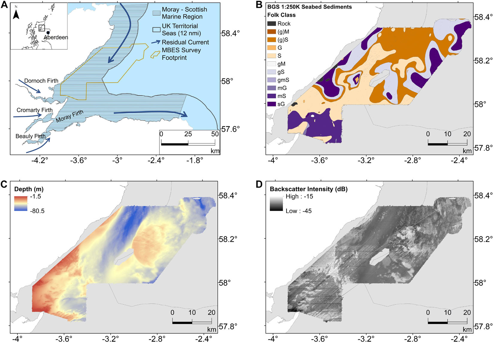
Figure 1. (A) Location map for the survey area within the Moray Firth on the east coast of Scotland. The inset map shows the location in the context of Scotland. (B) Folk sediment map from the BGS 1:250K Seabed Sediment product DigSBS250 (accessed from: https://mapapps2.bgs.ac.uk/geoindex_offshore/home.html). Folk codes as follows: (g)M, slightly gravelly mud; (g)S, slightly gravelly sand; G, gravel; S, sand; gM, gravelly mud; gS, gravelly sand; gmS, gravelly muddy sand; mG, muddy gravel; mS, muddy sand; sG, sandy gravel. (C,D) HI1150 MBES survey results. The rasters are presented at a 6 m × 6 m pixel resolution and the ArcGIS tool, “Focal Statistics” (circular neighbourhood, 3 m) has been applied to smooth noise. (C) Bathymetry (m). (D) Acoustic Backscatter Intensity (dB). The white area represents land, and the light-grey area represents the sea.

The seabed of the Moray Firth comprises a thin cover of Holocene sediments which are relict glacial and post-glacial accretions from offshore sources (Figure 1) (BGS (British Geological Survey), 1987; Reid and McManus, 1987). Following glacial melt at the start of the Holocene a rapid rise in sea level resulted in a source of lithic material to the area of predominantly sandy facies (Andrews et al., 1990). Sediments here are also sourced from fluvial contributions of the Dornoch and Cromarty Firths, limited to the south-west of the site and composed of muddy sands (Chesher and Lawson, 1983). Coarser, gravelly sands are found along the southern and northern coastlines in shallow water areas. Biogenic carbonate material is a final source of material which accumulates from calcareous seabed biota within the shallow coastal waters and which influences sediment composition (Holmes et al., 2004).

Sediment distribution is driven by local hydrodynamic regimes interacting with broader scale bathymetric variation. Due to the relatively shallow nature of the seabed, near-bed currents are mainly driven by wind and tidal interactions; the dominant current direction is from the north and north-east as NE Atlantic waters are channelled into the northern North Sea through the narrow channels between the Scottish mainland and offshore islands (Holmes et al., 2004).

Materials and Methods

To investigate the suitability of acoustic backscatter data to act as a proxy for sediment type, and thereby a predictor of OC on the shelf, we first ground truth an MBES survey and generate a sedimentary C dataset to examine relationships between backscatter, sediment type and OC. We fit LMMs for the two covariates, including the backscatter over a range of scales, and use geostatistical interpolation to predict OC across the footprint. We compare how well each of the covariates predicts spatial OC and calculate surficial stock estimates for the best models. We use an existing MBES dataset as a cost-effective way to re-purpose marine datasets. In this section, we describe each of these steps in detail; the flow diagram in Figure 2 provides a summary for reference.

FIGURE 2

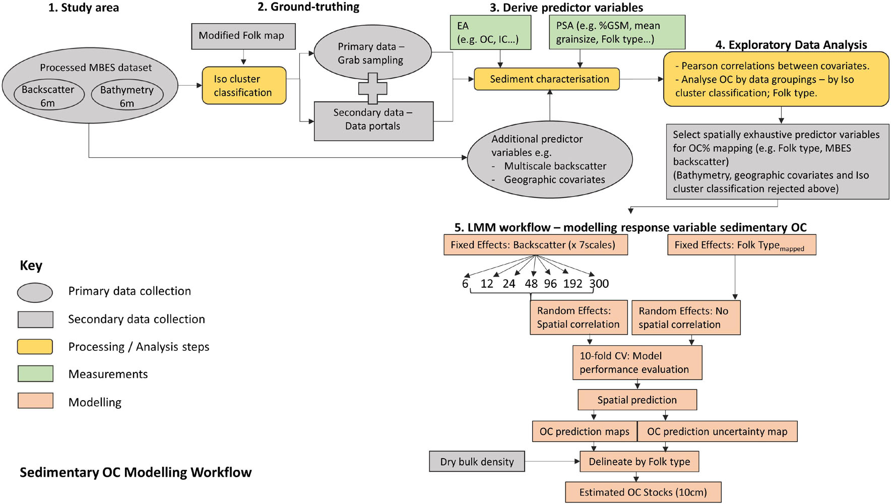
Figure 2. Flow diagram highlighting the order of the data collection and analysis steps used within this study.

Multibeam Echosounder Survey

The Civil Hydrography Programme (CHP) acoustic datasets are made available through the respective bathymetry¹ (UKHO hosted) and backscatter² (BGS hosted) Data Archive Centres. The “HI1150 survey: Tarbat Ness to Sarclet Head” MBES dataset was selected given that, firstly, physical sediment samples collected during the survey are archived at the National Geological Repository (NGR) in Keyworth, United Kingdom, and available to subsample for grain size and C analysis; and secondly, the typical sediment type (muddy-sands to sands) across the area was compatible to further sampling using a Day grab. These CHP MBES bathymetry and backscatter data are of high quality and have been processed to a very high standard, IHO Order 1a (IHO, 2020). This requires the data to meet strict accuracy and quality requirements, e.g., line spacing, sounding density, vertical accuracy, and cross-line calibration. The survey report is available from the UKHO Data Archive Centre. The 2006 MBES survey employed a Kongsberg Simrad EM710 (70–100 kHz) for the offshore leg, and a hull-mounted EM3002D (300 kHz) sensor for the inshore survey to account for two depth zones. A Trimble (RTK) GPS was used for positioning. Depth checks between the nadir beams of the MBES systems against a single beam echosounder agreed within a few centimetres, except in areas of rapidly varying terrain (e.g., rock or sand waves). Further to this, the backscatter data are processed to drastically reduce angle-range effects, ensuring accurate intensities are recorded across track. Bathymetry and backscatter data were processed using Caris HIPS/SIPS software. The total survey area covers approximately 2,640 km² (Figures 1C,D).

Multibeam Echosounder Data

Iso Cluster Classification

The bathymetry and backscatter data were classified using the unsupervised Iso Cluster tool in ArcGIS to inform our sampling strategy across the MBES survey footprint. These variables have shown strong discriminatory power for classifying seabed substrates (Calvert et al., 2015). Prior to classification, the bathymetry raster data were resampled to 6 m resolution for consistency with the backscatter dataset and both rasters were normalised from 0 to 1 (Calvert et al., 2015). We used the BGS 1:250K Folk sediment map (Figure 1B) to support our selection of five classes representing the four sediment types plus rock of the modified Folk classification (Long, 2006) (Figure 3). Equal numbers of sediment samples were proposed from each class with the sampling locations dispersed across the class footprint (Figure 3). Backscatter and bathymetry data were further processed to remove noise and account for potential sample location error, using the “Focal Statistics” tool in ESRI ArcGIS v10.7 (3-pixel × 3-pixel circular neighbourhood), prior to extracting the raster values at each sample location.

FIGURE 3

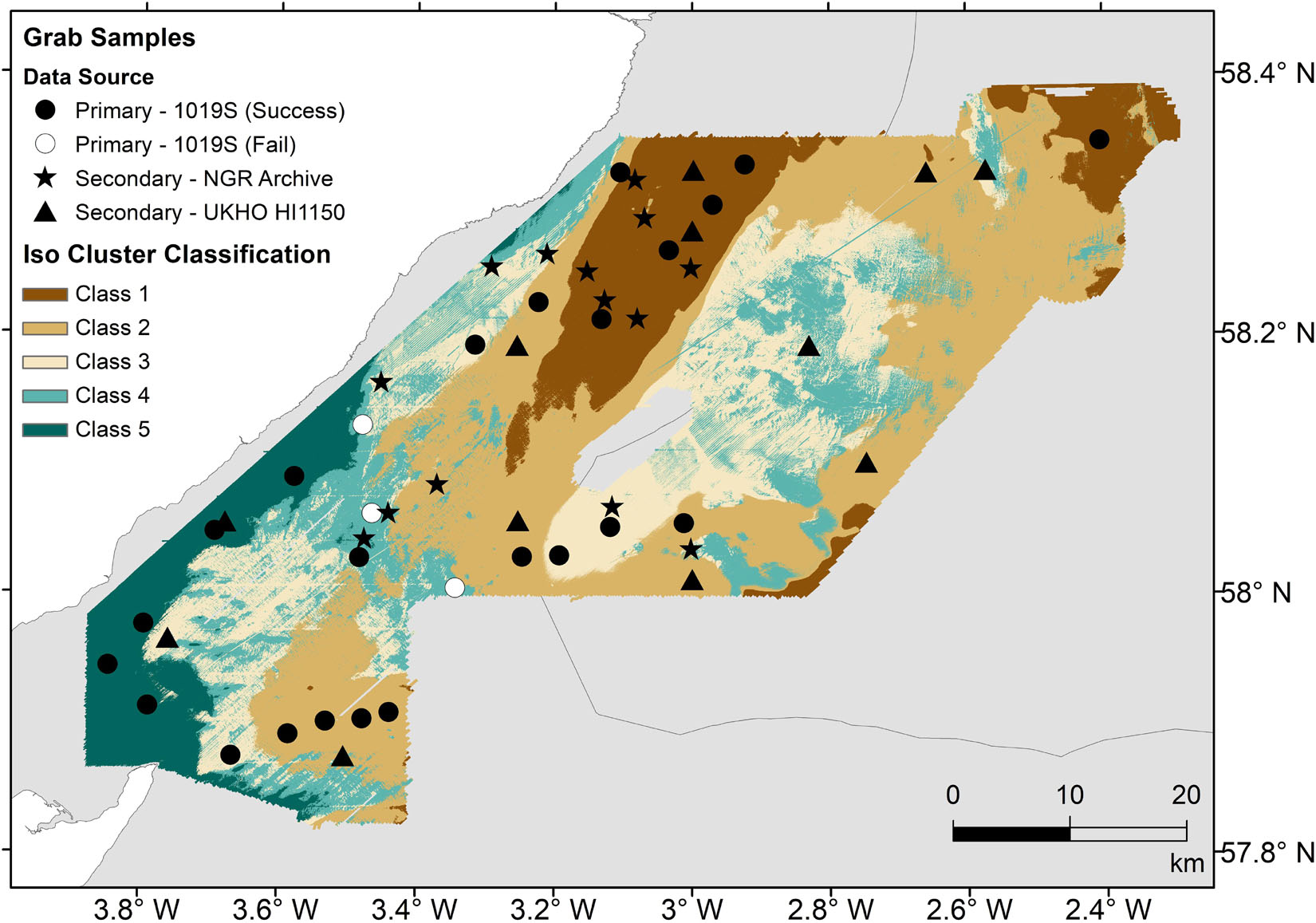
Figure 3. Classified map of the MBES survey using ArcGIS unsupervised Iso Cluster tool (five classes). Sample locations are shown. Primary samples were collected in July 2019. Secondary data samples were collected over multiple surveys (see Supplementary Table 1 for full details).

Multiscale Backscatter Data

Studies have shown that the spatial scales of terrain and ecological attributes are an important consideration in sedimentary modelling and mapping studies since different environmental processes operate at different scales (Wilson et al., 2007; Misiuk et al., 2018). To investigate if there was an optimum scale at which backscatter and OC were correlated, we re-gridded the original data (6 m resolution) to the following spatial scales: 12, 24, 48, 96, 192, and 300 m resolution using the bilinear algorithm in the ArcGIS Resample tool. The backscatter values at the sample point locations, and as averaged over a 300 m grid, were extracted and used as predictor variables in the modelling component (see section “Spatial Analysis – Linear Mixed Models”).

Sediment Characterisation

Primary Data Collection

Twenty-three grab samples were successfully collected by FRV Scotia (1019S) in July 2019 using a Day grab (0.1 m²) (Figure 3). Three grabs failed where the sediment was too coarse to sample (all within “Class 4”). A full list of samples and accompanying metadata is found in Supplementary Table 1. Samples were collected according to the United Kingdom’s Joint Nature Conservation Committee (JNCC) marine monitoring protocols (Davies et al., 2001). A full-depth scoop of sediment (∼10 cm depth) was collected from the Day grab, homogenised, and frozen until analysis.

Secondary Data

We supplemented our dataset using complementary secondary data spatially located within the MBES footprint. Physical material was subsampled from the NGR. This included the 11 retained samples collected during the HI1150 MBES survey and additional archive material collected during national seabed surveys from the 1970s (Fannin, 1989). We also searched national databases (e.g., ICES) for sedimentary datasets with associated OC and grain size information, however, due to differences in analytical methods and reporting formats of the OC sediment fraction and grain size statistics, we decided to only use the physical secondary samples available for laboratory analysis, to maintain consistency with our primary data. There will be some uncertainty in OC amounts from archive samples attributable to the possible loss of labile material during long-term storage, which could manifest in an underestimation in OC predictions. We also note that the location uncertainty of archive samples is approximately 100 m because these were collected prior to the availability of Global Positioning Systems (Lark et al., 2012). Despite the uncertainties, the increased dataset nevertheless allows us to better characterise the regional sedimentary properties. An inventory of secondary data is found in Supplementary Table 2 and includes a further 29 samples.

Carbon Analysis

Sediment samples were oven-dried at 50°C until constant weight, cooled, and ground to a homogenous powder. 40 mg ± 5 mg of sediment was weighed out into pre-baked steel crucibles. Carbon analysis was carried out using an Elementar SoliTOC Cube Elemental Analyser. This instrument measures in situ organic and inorganic C within a sample, thus the typical pre-acidification step to remove carbonates is not required to measure the organic component. This is advantageous for coastal sediments comprising inorganic material because the acidification step can result in loss of sample through effervescent reaction (Verardo et al., 1990). The machine was calibrated against the standard reference material, B2290 (TOC/ROC/TIC silty soil standard) from Elemental Analysis, United Kingdom. The standard measurements deviated from the reference value by: TOC = 0.14%; ROC = 0.003%; and TIC = 0.29%. The measured C was normalised to the proportion of the sediment composition <2 mm. This represents the fraction of the bulk sediment viable for analysis; we assume that there is no OC associated with the sedimentary fraction >2 mm (i.e., “gravel” or rock).

Sediment Grain Size

Particle size analysis was undertaken for the 23 primary sediment samples using the protocol outlined in Mason (2011) to split the bulk material into coarse (>2 mm) and fine (<2 mm) components prior to analysis. The coarse material was sieved at ½ phi intervals (5.6, 4.0, 2.8, and 2.0 mm). The <2 mm fraction was analysed in a Coulter LS230 laser granulometer. The machine was calibrated using two sizes of glass bead reference standards (Vasquashene C100 and Vasquashene 590/840). Samples were treated with 3 ml of 5% Calgon solution to aid dispersion of aggregates prior to analysis (Blott et al., 2004). The results from the fine and coarse fractions were combined into a full particle size distribution as per Mason (2011). Grain size statistics were derived using GRADISTAT (Blott and Pye, 2001), although we only consider mean grain size in this study.

Dry Bulk Density

The dry bulk density (DBD) values of the sediment types have been derived from Smeaton et al. (2021) who collated sedimentary DBD data from across the United Kingdom Exclusive Economic Zone (EEZ). Where available, we first extracted region-specific data for the Moray Firth and aggregated the higher sediment classifications into the modified Folk sediment types (Kaskela et al., 2019). The average DBD value for each type is used in C-stock calculations and can be found in Supplementary Table 3.

Observed Sediment Type – Harmonising the Data

We only had access to the bulk sediment of the 23 primary grab samples and therefore could only generate full particle size distributions for these samples. The secondary sediment samples were available for subsampling in conservative amounts from the NGR archive, and we could not assume the sub-samples were representative of the bulk sediment to establish a quantitative grain size breakdown. We instead relied on composition metadata available from the BGS Offshore Geoindex³, to harmonise the primary and secondary data by deriving a modified Folk classification based on the % gravel, % sand, and % mud composition of each sample (Kaskela et al., 2019; Smeaton and Austin, 2019). Every data point has thus been described according to the modified 5 Folk classification (Mud-muddy sand; Sand; Mixed sediment; Coarse sediment; and Rock) (Kaskela et al., 2019). This allowed us to investigate how the composition of sediment affects the acoustic backscatter response.

Modified BGS Folk Sediment Map

As above, we converted the United Kingdom seabed Folk sediment polygon shapefile (1:250,000) (BGS (British Geological Survey), 1987) into a modified Folk sediment raster within ArcGIS by aggregating and reclassifying the default 16 Folk classes into 5 Folk classes based on Kaskela et al. (2019). The raster was projected into UTM Zone 30N and resampled to a 300 m resolution to align with the maximum backscatter raster scale (see section “Multiscale Backscatter Data”). We cross-checked the observed sediment type at each grab sample location (see section “Observed Sediment Type – Harmonising the Data”) against this reclassified sediment map to see how well it represented the sediment types described by the point sample data. Values of modified Folk type were extracted at each sample location (“mapped” Folk opposed to “observed” Folk) and used as a covariate within the spatial models. The modified Folk raster was also used as a continuous predictor variable for OC in our spatial predictions (see section “Spatial Analysis – Linear Mixed Models”).

Exploratory Analysis – Drivers of Organic Carbon Variation

Spatial information was extracted for each sample location using ArcGIS V10.7 including, geographical northing and easting and distance from the coast (calculated as the planar distance in metres from the target sample to the closest point on the coastline). These variables are included as potential predictors of sediment type and OC (Diesing et al., 2017). The appropriateness of using MBES and sedimentary data as explanatory variables to spatially predict OC was explored in the following ways; (i) by comparing the summary statistics of the sample data grouped by Iso Cluster class and by modified Folk type (Supplementary Tables 4, 5) and (ii) by exploring statistical associations between sedimentary properties and backscatter variables using Pearson correlation coefficients (Supplementary Figure 1 and Supplementary Table 6) (Serpetti et al., 2012). The relationship between modified Folk type, a categorical variable, and OC was compared using a one-way analysis of variance (ANOVA) (Supplementary Table 7). These analyses provided the supporting evidence for whether backscatter was a viable proxy for characterising sediments in this area (i.e., do sediment types have characteristic signatures?), and for insights into the significant predictors of OC here.

Spatial Analysis – Linear Mixed Models

We applied geostatistical methodology (Webster and Oliver, 2007) to explore how the observed relationships between OC and its drivers of variation could be used to map OC across our study region and how predictions of OC and their uncertainty could be upscaled to the entire study region. Non-spatial statistical methodologies such as linear regression require the assumption that the model errors or residuals are independent. In contrast, spatial analyses acknowledge that these residuals could be spatially correlated (i.e., residuals from proximal locations are more likely to be similar than those from disparate locations). This means that there is a spatial pattern to the observed data beyond that which can be explained by the covariates. This unexplained spatial pattern can be predicted using geostatistical methods (Webster and Oliver, 2007) thus improving the accuracy of the maps that result. The spatial correlation can also lead to the underlying model consistently under- or over-estimating the true values across broad portions of the study region. This in turn implies that the uncertainty of upscaled predictions of OC (e.g., the average across the study area) can be larger than if the residuals were independent.

We explored the spatial relationships between OC and the strongest drivers of variation as per the Pearson correlation coefficients, by estimating a series of LMMs by residual maximum likelihood. This is a commonly used method in terrestrial spatial C stock studies (Lark et al., 2006; Rawlins et al., 2009). LMMs divide variation in the modelled variable between the fixed effects (i.e., an assumed linear relationship between the response variable, in this case OC, and the explanatory covariates) and a random-effects component (i.e., the variation in the model residuals which can be spatially correlated). A comprehensive explanation of this type of geostatistical model can be found in Lark et al. (2006).

The model covariates must be known at all locations where the OC is to be predicted. We thus used the “mapped” modified Folk sediment type as a proxy for mean grain size and composition data in the fixed effects and compared its performance with the backscatter data processed to different scales. At the model estimation and validation stage, we also consider the “observed” Folk class to explore the effectiveness of this predictor if it were known precisely at each location. This covariate cannot be used to predict OC at locations where it was not measured, however. For each covariate, we consider both independent and spatially correlated random effects. In the geostatistical literature, independent residuals are said to have arisen from a pure nugget model. We use an exponential function (Webster and Oliver, 2007) to represent the degree of spatial correlation when it is present in the model. The appropriateness of the different combinations of fixed and random effects was assessed via the Akaike Information Criterion (AIC, Akaike, 1973) which weighs model complexity against model fit. The model which leads to the lowest AIC is thought to have the appropriate degree of complexity to best model the observed data (Villanneau et al., 2011).

The best-fitting models were used to predict OC and its uncertainty across the study region using the best linear unbiased predictor (BLUP) (Lark et al., 2006). This is a spatial interpolation method, sometimes referred to as kriging, which combines the fixed and random effects. We also simulated 1,000 realisations of OC according to each fitted model using the Cholesky decomposition approach (Webster and Oliver, 2007). Each of the realisations reflects the degree of spatial correlation in the estimated model. If the average OC across the study region is calculated for each realisation, then the variation between these averages reflects the uncertainty in predicting OC at this scale.

The relatively small number of samples in this study meant it was difficult to split the data into a training and validation set. Instead, the models were validated by a 10-fold cross-validation procedure (Webster and Oliver, 2007). In this process, a tenth of the observations are removed from the dataset and the other observations are used to predict OC at the locations of those that have been removed. The process is repeated 10 times with different observations removed each time so that each observation is removed once. The predicted values are compared with the observed values and the bias can be assessed by calculating the mean error (ME):

$$\text{ME}=\frac{1}{n}\sum _{i=1}^n\left\{z\left(x_i\right)-\widehat{z}\left(x_i\right)\right\},$$

and the accuracy by calculating the root mean squared error (RMSE),

$$\text{RMSE}={\left[\frac{1}{n}\sum _{i=1}^n{\left\{z\left(x_i\right)-\widehat{z}\left(x_i\right)\right\}}^2\right]}^{\frac{1}{2}},$$

or the correlation between predicted and observed values, where z(x_i) is the observed OC and $\widehat{z}\left(x_i\right)$ is the prediction of OC at location x_i and n the number of observations.

In addition to a prediction of OC at each location, the BLUP also produces a measure of uncertainty of the prediction referred to as the prediction or kriging variance, an important consideration for decision-makers (Lark et al., 2012). The degree to which the kriging variances ${\widehat{\mathrm{\sigma }}}^2$ relate to the prediction uncertainty can be explored by calculating the standardised squared prediction errors (θ) at each site:

$${\mathrm{\theta }}_i=\frac{{\left\{z\left(x_i\right)-\widehat{z}\left(x_i\right)\right\}}^2}{{\widehat{\mathrm{\sigma }}}^2\left(x_i\right)}.$$

If the random effects are normally distributed and the LMM correctly describes the variation of OC, then the expected mean and variance of the θ_i are equal to 1.

Organic Carbon Stock Estimates

Surface (10 cm) OC stock estimates were calculated for the best-fitting model surface maps using the methodological steps outlined in Burrows et al. (2014). The modified Folk class raster was first converted into a corresponding map of average DBD using the values identified from section “Dry Bulk Density.” Combined with the maps of predicted OC, OC stocks and densities were derived per pixel area. For each spatial model, we calculated the OC stock over each Folk class area by aggregating the predicted OC mass for all relevant pixels. The uncertainty of these stocks was determined by repeating the stock calculation process for each of the 1,000 realisations of OC simulated from each LMM. The standard deviation of the stock predictions that resulted approximates the standard error. This approximate standard error does not account for uncertainty in estimating the DBD for each Folk class.

Results

Data Characteristics

Backscatter Signal

The backscatter data (Figure 1D) highlight discrete areas of high intensities within an otherwise generally homogenous signal, broadly reflecting the sediment structure described in section “Regional Setting.” High backscatter intensities follow the coastline, coincident with rock and coarse sediments (Figure 1B). The area overlying the Smith Bank is characterised by higher backscatter (∼−16 to −21 dB), likely a signature of the coarser sand and gravel material described by previous surveys (Holmes et al., 2004). There are additional areas of high backscatter (∼−16 to −23 dB) associated with bathymetric-high features known as drumlins (streamlined subglacial landforms comprised of coarse and over-consolidated sediments), leaving the Dornoch Firth. The upstanding ridges will be more exposed to currents and therefore likely to consist of coarse-grained material, flanked by winnowed finer sediments within the troughs. Much of the remaining area is represented by lower backscatter intensities ranging between −28 and −34 dB correlating with observations of sand-dominant sediment facies (Andrews et al., 1990).

Sediment Type

Our grab samples were predominantly classified as sands and muddy sands, with a smaller proportion classified as coarse and mixed sediments (Figure 4 and Supplementary Table 1). Generally, it is difficult to sample a coarser sediment matrix successfully and these sediment types are often under-represented in sedimentary C studies. The three failed grabs during 1019S (all within “Class 4”) were likely due to coarse sediments. This assumption is supported by Figure 4, which clearly delineates the coarse sediment found within “Class 4” compared to the other classes. “Class 5” has a varied mixture of sediment types which could indicate poor sorting of sediments closer to the coastline. Despite having different compositions, the mean grain size of sediments collected within Classes 1, 2, 3, and 5 (following removal of outlier GB12) are broadly similar (∼150 μm) and classify as fine to medium sands with a mean backscatter intensity (∼−31 dB ± 1) (Supplementary Table 4). The mean grain size for “Class 4” is significantly higher (∼2 mm) characterised as a coarse sediment and matched by high mean backscatter intensity (−20.4 dB).

FIGURE 4

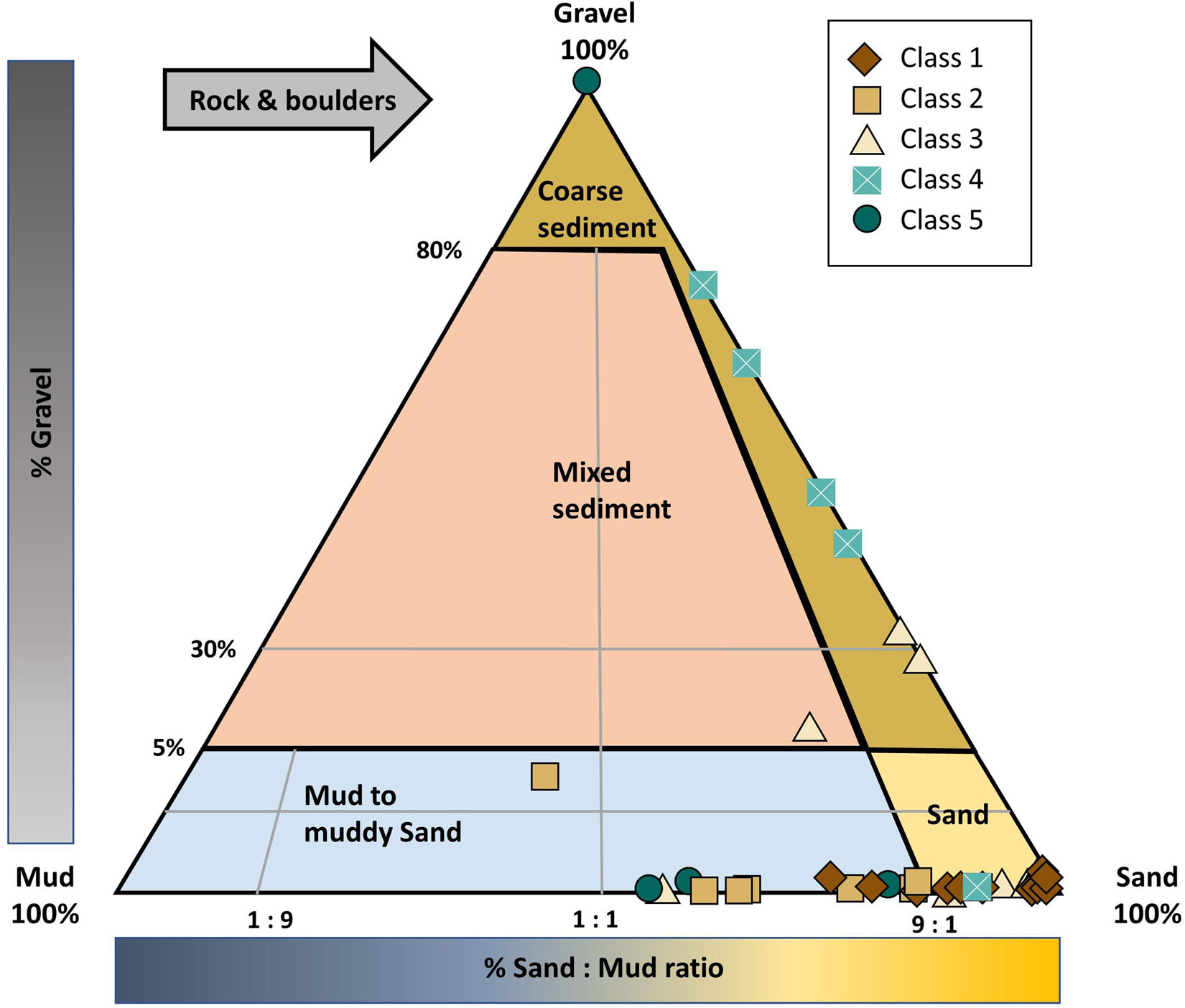
Figure 4. Sediment samples with % gravel, sand, and mud data mapped to a modified Folk classification (four classes + rock) as proposed by Kaskela et al. (2019) to enable harmonisation between multiple datasets. Samples are grouped by Iso Cluster class.

We chose to reclassify our primary grab samples to a modified Folk class (see section “Observed Sediment Type – Harmonising the Data”) to incorporate secondary data in our study. The observed Folk type broadly agrees with the modified Folk map over the study area (Figure 5), with 60% overall accuracy (Supplementary Table 8). The main source of disagreement comes from grab samples of muddy sands being incorrectly classed as sands and coarse sediments by the BGS Folk map indicating there is heterogeneity over finer scales than is captured by broad Folk sediment classifications.

FIGURE 5

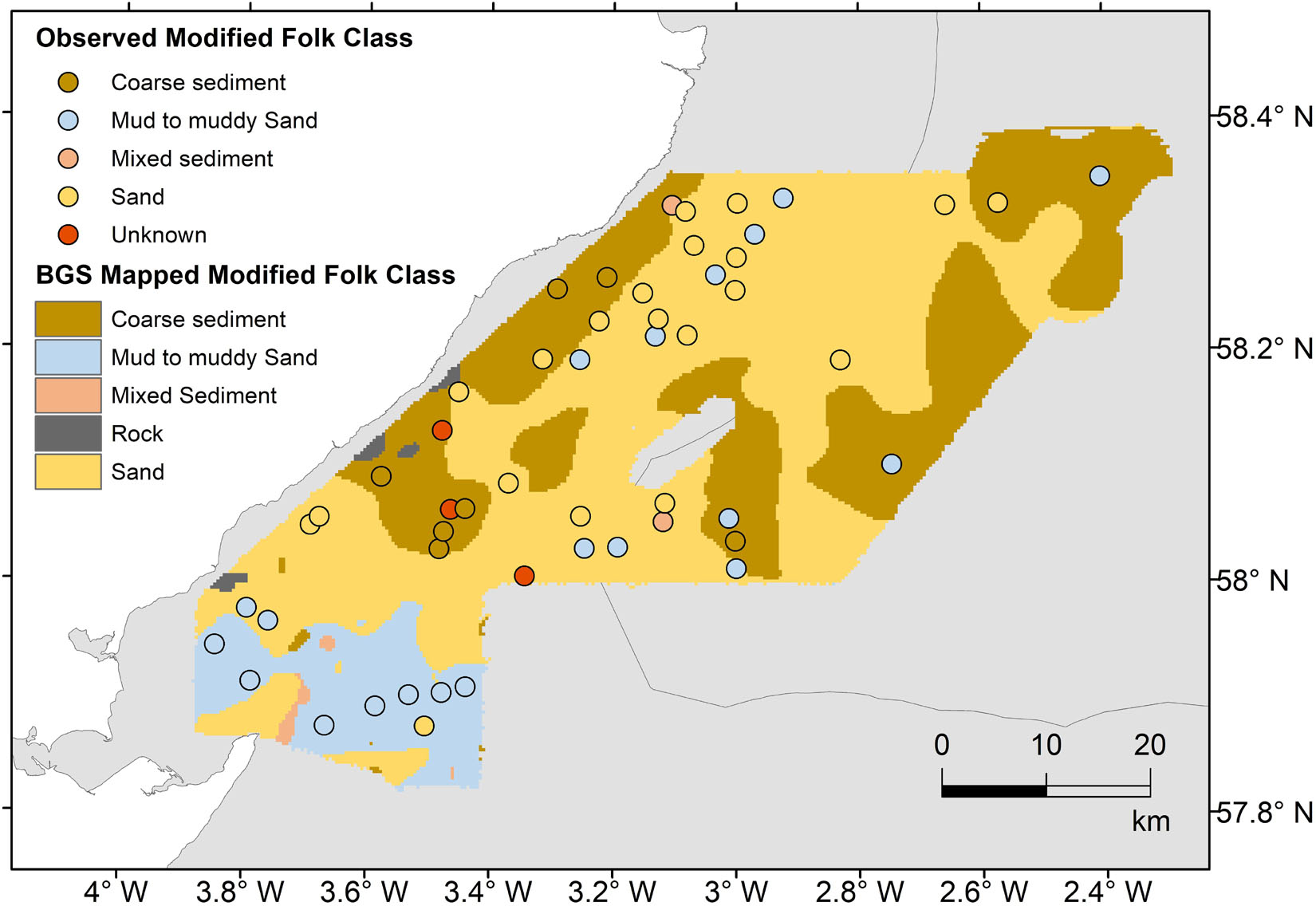
Figure 5. Observed sediment type from all grab samples overlaid on the modified BGS Folk sediment map (adapted from DigSBS250). Agreement statistics between observed and mapped classes are shown in Supplementary Table 8.

Sedimentary Organic Carbon

Organic carbon values are consistent with other studies from the coastal shelf environment on the east coast of Scotland (Serpetti et al., 2012); values range from 0 to 1.55% content, with an overall mean value of 0.87% and a standard deviation of 0.37% (Supplementary Table 1). Enriched OC values are found closer to the estuary, characterised by muddier sediments, and within the deeper water (defined by “Class 1”) suggesting that depth could be a factor in OC accumulation (Supplementary Table 4). “Class 4” has the lowest range of values recorded – the average OC content within this class is 0.65% ± 0.41 (Supplementary Table 4) and mean grain size ∼2 mm. When grouped by Folk type (Supplementary Table 5) the muddy sands are enriched in OC% (mean = 1.04% ± 0.27) and coarse sediments have the lowest average value at 0.38% ± 0.27. Sands have the largest variability in OC% (between 0.18 and 1.31%) with higher values overlapping those found in the muddy sands.

Exploratory Analysis

Effectiveness of Iso Cluster Classification

The objective of the unsupervised Iso Cluster classification of MBES bathymetry and backscatter was to identify distinct seabed substrates to guide a representative sampling strategy. Grouping the sample variables by Class highlights some issues with our approach. The bathymetry data appeared to drive the final classification demonstrated by each class having a distinct depth range, except for Classes 3 and 4 (Figure 6A). The distinction between Class 3 and 4 was subsequently made using backscatter intensity. However, in this study, bathymetry shows limited discriminatory power to separate between sediment types (Figure 6B) indicating that our classification approach did not meet the objectives. This could be due to limited data, and it is possible that finer-scale sampling would have shown a response to small-scale bathymetric and geomorphological variation. “Class 4” (Figure 6A) is an exception and is distinctive from the others exhibiting similar characteristics to those of coarse sediment (Figure 6B) demonstrating the strong effect of increased grain size on acoustic backscatter (Goff et al., 2000).

FIGURE 6

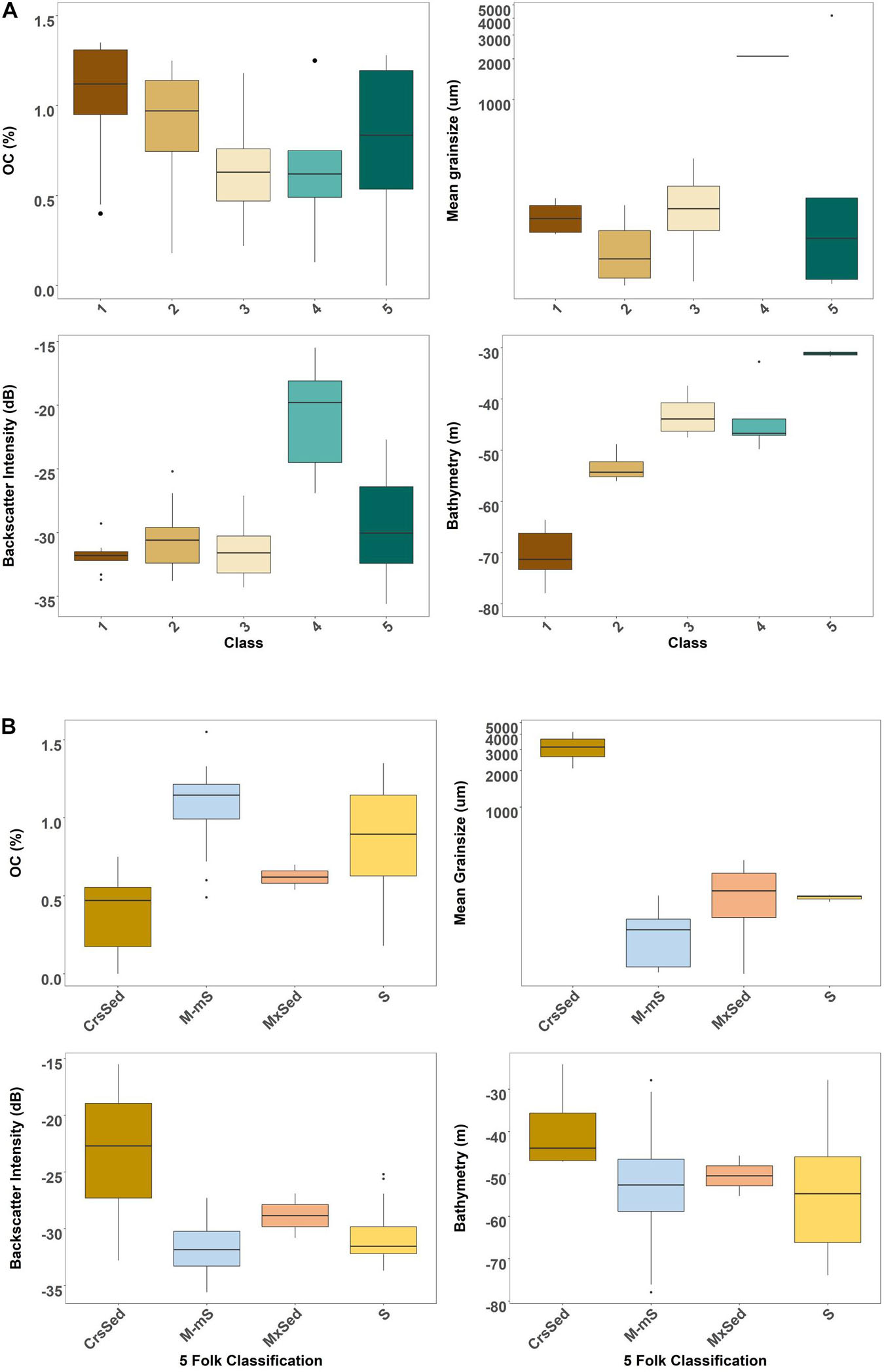
Figure 6. Box plots characterising the core variables from the ground truth samples by (A) Iso Cluster classification and (B) modified Folk sediment type (Key for modified Folk type: CrsSed, coarse sediment; M-mS, muds to muddy sands; MxSed, mixed sediment; S, sand).

Grouping the data instead by sediment type (n = 49) shows more distinct trends (Figure 6B). Coarse sediments have distinct signatures for all variables specifically, the lowest OC% values, a mean grain size >2 mm, the highest backscatter intensities, and are within shallower depths. Mixed sediments are characterised by slightly larger mean grain sizes than sands due to the presence of gravel. This is also reflected in higher backscatter intensities for mixed sediments relative to muddy sands and sands. Despite having distinctly different mean grain sizes (note that mean grain size is only available for (n = 23 samples), muddy sands and sands are characterised by similar mean backscatter values (∼32 dB) and depth ranges. Backscatter has thus provided a distinction between coarse sediments from muddy sands (M-mS) and sands (S); however, these sediment types are indistinguishable from each other based on backscatter intensity alone. Mean grain size (n = 23) is a more useful indicator in this respect than sediment type.

Other than “Class 4” (coarse sediment), the Iso Cluster classification has not been able to differentiate sediment types, and OC contents satisfactorily. Thus, we have chosen not to use the Iso Cluster classification as a predictor (categorical) variable in further analysis and instead, we use Folk sediment type which demonstrates better coupling to OC content and backscatter.

Predictor Variable Correlations

Backscatter is significantly correlated with mean grain size (r = 0.72) and most influenced by the gravel content (r = 0.76) (Figure 7A and Supplementary Table 6), correlations that are in keeping with other studies (Goff et al., 2000; Sutherland et al., 2007; McGonigle and Collier, 2014). OC has a significant, negative correlation with both mean grain size (r = −0.68) and with backscatter but this is much weaker (r = −0.47). The relationship appears to be driven in part by sediment composition highlighted by relationships with both % gravel (r = −0.65) and % mud (r = 0.48) (Figure 7B and Supplementary Figure 1). Backscatter does not separate OC values around −30 to −34 dB (Figure 7B), which is problematic because this backscatter range corresponds to varying compositions of muddy-sands and sands represented by similar mean grain size but with different associated OC values, ranging from ∼0.3 to 1.4%. However, despite our low sample numbers, we do see the general trends that we would broadly expect given the empirical relationships between these predictor variables (Hunt et al., 2020); increased backscatter intensities correlate to reduced OC contents as a function of sediment type becoming coarser. There are clearly environmental complexities, beyond which our dataset parameters can elucidate.

FIGURE 7

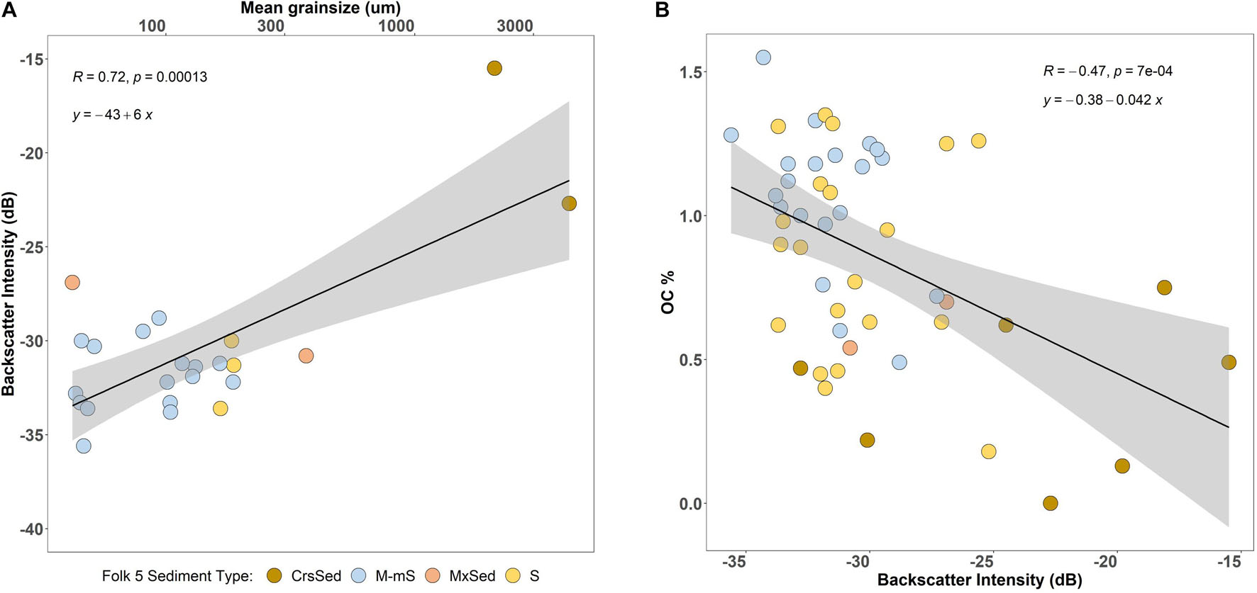
Figure 7. (A) Backscatter correlated with mean grain size (n = 23) grouped by Folk sediment type and (B) OC% correlated with backscatter (dB) (n = 49) grouped by Folk sediment type to highlight the complexity within the correlations between these variables (Key for modified Folk type: CrsSed, coarse sediment; M-mS, muds to muddy sands; MxSed, mixed sediment; S, sand).

Water depth is weakly correlated to OC (r = −0.3) with no overall trends and therefore depth is not a reliable predictor of OC in this study (Supplementary Figure 1). Geographic covariates, distance from the coast, easting, and northing, are not correlated with OC and not used further.

Spatial Analysis: Linear Mixed Models

In total, nine LMMs of OC variation with single fixed effects were estimated as summarised in Table 1. All model validation statistics can be found in Supplementary Table 9. The lowest AIC is achieved by using the observed Folk classification derived from our samples as the fixed effects, followed by the classified Folk map values. Inclusion of sediment type and backscatter information as a covariate (fixed effect) improved the model performance by 17–19% (mapped and observed) and 14%, respectively, compared to the constant fixed effect model according to the relative decrease in the RMSE values (Supplementary Figure 2). Of all the scales for backscatter, the data at the 48 m resolution lead to a more accurate model, indicating that backscatter resolution may be an important consideration for OC mapping, however, the differences in accuracy are modest and more data would be required to support this hypothesis. The fixed effects selected to spatially predict the OC were M5b (backscatter − 48 m) and M8b (Folk-mapped) because these variables are known across the study site.

TABLE 1

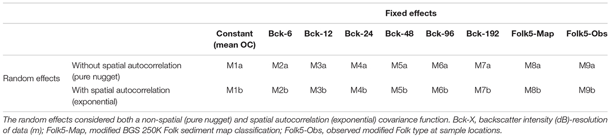
Table 1. Matrix summarising linear mixed model permutations fitted to the observed data to predict OC%.

While including exponential spatial correlation in the random effects did not improve any model fits according to the AIC alone, it does lead to small improvements in the model accuracy (Supplementary Table 9). Further, the upscaled prediction uncertainty values for the pure nugget are unrealistically small, approximately 1% of the total stock estimate (Supplementary Table 10). This results from a cancelling-out effect of positive and negative errors at different prediction locations. The failure of the spatially correlated random effects to improve the AIC is likely to reflect the relatively small sample size meaning that there is limited evidence to assess the spatial correlation. It cannot be interpreted as evidence of an absence of spatial correlation. We therefore included spatial correlation in our spatial predictions of OC (Figure 8).

FIGURE 8

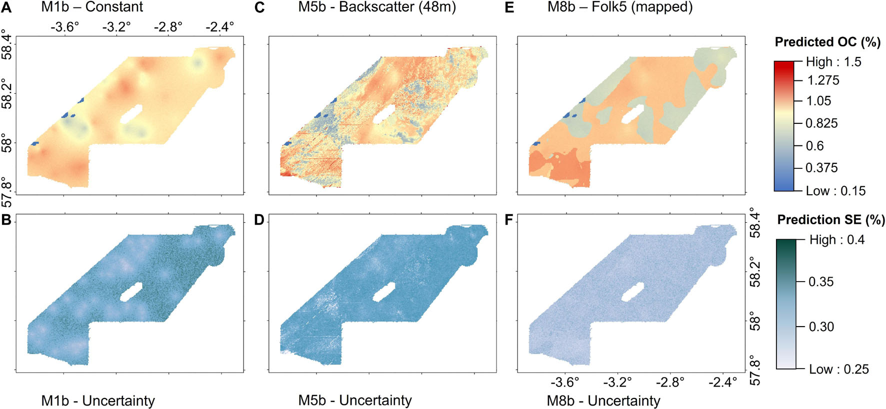
Figure 8. Predicted spatial distributions of OC% for the different LMMs (top row) and corresponding prediction uncertainties given by the model standard errors (bottom row). (A,B) Model M1b: Constant fixed effects (mean OC). (C,D) Model M5b: backscatter at 48 m resolution. (E,F) Model M8b: Mapped modified Folk class. All models have exponential random effects. The maps are projected in ETRS89/UTM zone 30N (EPSG:25830) and have a raster resolution of 300 m.

Only one of the observed OC values was made at a location with a “Mixed sediment” mapped Folk classification. Therefore, the expected OC % for the “Mixed sediment” class could not be estimated. For the purposes of spatial prediction, the expected OC % for this Folk class was assumed to equal the average of the expected values for the other three classes. Mixed sediment covers around 1% of the study area so this assumption is unlikely to substantially influence the predicted maps or site-wide stocks.

All models quantify the uncertainty satisfactorily according to the variances of the θ_i values which are close to 1; the spatial variation of this uncertainty can be seen in the standard error maps in Figure 8. Highest uncertainties arise from the constant fixed-effects model. The predicted OC using M5b ranges from 0.2 to 1.4% and is highly variable across the site. Lowest values of OC and associated prediction uncertainty are concurrent with high intensities in backscatter characterised by coarse sediments and rock (assumed to be 0%). For M8b, predicted OC shows very little variation within Folk sediment type boundaries and ranges from approximately 0.5–1.2%, the highest values characterised by the area of muddy-sands. The maps have relatively large standard errors which reflect the large degree of small-scale variation in OC. These uncertainties could be reduced if more data were collected.

Organic Carbon Stock Calculations

Table 2 outlines the estimated OC stocks calculated from the spatial predictions of OC for model M5b (estimated 3.00 ± 0.159 Mt OC) and model M8b (estimated 3.08 ± 0.164 Mt OC). The total OC stocks derived from the two models are within the prediction error of each other, differing by approximately 0.08 Mt. The Folk model predicts the higher stock value presumably a result of not capturing finer-scale sediment heterogeneity with sediment boundaries (Figure 5). The limitation of this backscatter dataset to differentiate between sands and muddy sands (similar intensity values) could be leading to an under- and over-estimation for OC in muddy-sands and sands, respectively (Figure 7). Both models agree that sands contribute most to the total stocks (∼60–66%) due to their coverage. Estimated values for OC density are within the values estimated by other studies for United Kingdom coastal sediments, although in contrast to Smeaton et al. (2021), the two models predict that sands have the highest OC density rather than the muddy sediments (Table 2).

TABLE 2

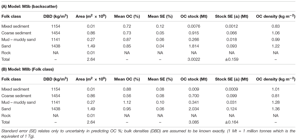
Table 2. Calculation of organic carbon stock using (A) predictions from the linear mixed model with backscatter at 48 m resolution as a fixed effect covariate including exponential random effects and (B) predictions from the linear mixed model with mapped Folk class as a fixed effect including exponential random effects.

Discussion

We have explored the potential of using archived MBES backscatter data in combination with primary and secondary ground-truth data to map OC at high resolutions over a regional area. We see promising trends between the predictor variables, yet the correlation between backscatter and OC is relatively weak, which suggests that backscatter cannot be solely used to predict OC. However, we show that the inclusion of this variable improves the carbon prediction accuracy or equivalently reduces the number of OC measurements required to achieve a specified precision. Comparing two exhaustive parameters, sediment type and backscatter, we have modelled two regional distribution maps of OC over an MBES footprint (2,640 km²) within the Moray Firth with spatially explicit uncertainties (Figure 8). We have used these maps to estimate surficial OC stocks across the area (Table 2). The stock estimates are in good agreement with each other; however, the spatial distribution pattern of OC varies. This is a result of the differences in how the covariate data were acquired. The BGS Folk sediment map is currently the United Kingdom’s best national seabed map based on interpolated point data and expert judgement, whereas backscatter is a form of high-resolution remote sensing. Further samples and additional complementary predictor variables are needed to resolve the finer-scale variability of OC and to understand which of the maps is most representative; this would also serve to reduce the relatively large standard errors of OC (Figure 8). In this section, we discuss the limitations and opportunities of acoustic backscatter as a predictor variable for OC. We briefly analyse the spatial distribution of OC of this Scottish east coast embayment and its role in C-processing, and we consider the implications for such OC maps in seabed management and C-accounting frameworks.

Acoustic Backscatter as a Predictor of Sedimentary Organic Carbon

While backscatter has a significant, negative correlation with the OC content in surface sediments (Supplementary Table 6), the strength of the relationship is relatively weak, and thus offers limited power to predict OC directly. This is a similar finding within habitat or substrate mapping studies using MBES data, which show that backscatter can improve models as part of a suite of predictor variables (De Falco et al., 2010; Lucieer et al., 2013). The inclusion of backscatter in the geostatistical model M5b leads to a prediction accuracy improvement for OC of approximately 14% This is a promising finding and is similar to improvements seen in substrate mapping accuracy when backscatter variables were incorporated (Lucieer et al., 2013; Biondo and Bartholomä, 2017). The resolution of the backscatter variable did not impact the overall performance of the LMMs, however, this does not mean that there is no difference and is likely a function of the limited sample size for the survey area. High-resolution backscatter data as a spatial covariate has the potential to increase the resolution of OC maps (Hunt et al., 2020). Fine-scale variability can be incorporated into these maps beyond which can be accounted for by current sediment maps (Smeaton et al., 2021).

The backscatter data differentiates between areas of coarse and fine sediments; however, it is not able to distinguish between muddy-sand and sandy sediments. Distinguishing between coarse and fine sediments is still a useful finding with respect to OC mapping because OC varies as a function of sediment type (Hedges and Keil, 1995), with significantly lower quantities of OC within coarse sediments (Figure 6). High-intensity backscatter is characteristic of coarse or poorly-sorted material (Collier and Brown, 2005; Biondo and Bartholomä, 2017), which are likely to result from dynamic or erosive processes, and therefore unimportant areas for C storage. This visual aid can help prioritise ground-truthing toward the finer-grained sediments associated with deposition and enrichment in organic matter (Diesing et al., 2021). The difficulties of the backscatter to delineate between finer materials could be due to a limitation of the MBES survey technology and post-processing methods employed over a decade ago, however, similar challenges have been identified in very recent studies, indicating that further development is still required within this field (Diesing et al., 2020). As a result, there are likely to be some systematic over- and under-estimations of OC for sands and muddy-sands, which have similar intensities. Sediment composition can also cause conflicting interpretation of the backscatter signal and OC content. For example, a muddy gravel can have a very high backscatter signal, particularly as gravel or shell hash disproportionately affects the scattering effect (Goff et al., 2000, 2004), but counter-intuitively, also a relatively high OC content governed by the presence of mud (Serpetti et al., 2012). Increased ground-truthing or camera-tow coverage would help to better characterise the sedimentary environment in these areas (Hunt et al., 2020).

The dominant oceanographic characteristics of the inner Moray Firth are of a dynamic coastal system and the seabed is comprised of glacially relict, re-worked sediments (Reid and McManus, 1987). These factors will influence OC quantity and quality and could help to explain why the correlation between backscatter intensity as a proxy for OC is less convincing than backscatter as a proxy for sediment grain size. There are numerous variables that can influence the availability of OC within sediments including, oxygen penetration levels (Janssen et al., 2005; Hicks et al., 2017), water temperature (Burdige, 2011), sedimentation rate (de Haas et al., 1997), reactivity of OM (Burdige, 2007; Bianchi, 2011), disturbance levels (e.g., through benthic fishing actvities: De Borger et al., 2020), and age/transportation times (Bao et al., 2019), which cannot be explained by backscatter alone. Equally, the relationship between backscatter and sediment type is complex (Diesing et al., 2020) and return signals can be influenced by the survey itself, including factors such as instrument type and acoustic frequency settings, weather conditions, and data processing techniques, and by physical environmental characteristics including sediment density and bioturbation from benthic fauna (Feldens et al., 2018).

Nevertheless, our results show that when backscatter measurements are combined with OC values within a geostatistical framework, the precision of the carbon predictions improves, and this method allows the prediction uncertainty to be quantified. In the absence of appropriate or exhaustive sedimentary datasets, our models show that acoustic backscatter data could be used to generate an improved picture of the spatial distribution of OC with appropriate ground-truthing. The backscatter data highlight some interesting finer-scale variations that could provide insights into geomorphological features and sedimentary processes, which may also have implications for carbon storage, such as sand ripples, moraines, or trenches.

Folk Type as a Predictor of Sedimentary Organic Carbon

Sediment Folk type was a stronger covariate than backscatter for predicting OC in this study, and is commonly used within sedimentary OC studies (Smeaton et al., 2020), however, there are limitations with using such categorical data. Much of the United Kingdom archive sediment data is classified using the Folk scale based on broad composition information (Lark et al., 2012) which can be associated with a wide range of OC values. The current BGS 250K Folk sediment map for the United Kingdom doesn’t pick up the heterogeneity in sediment type at smaller scales as highlighted by the 60% agreement between our observed samples and the Folk map (Figure 5). Sediment heterogeneity can have a large influence on C storage and should be accounted for Smeaton and Austin (2019). Areas of disagreement may be attributed to analytical improvements in sediment grain size detection for fine sediments (e.g., with laser sizing technology available) and/or legacy sample location inaccuracies which did not have the benefit of Global Positioning Systems (GPS) (Lark et al., 2012). In addition, large temporal differences exist between the samples collected in the 1970s, from which the BGS Folk sediment map was derived, compared to the samples for this study, during which time there is likely to have been considerable sediment movement. The improvement in LMM prediction accuracy of OC using sediment type is a clear indication of the importance of understanding sediment type and distribution. The confidence in substrate maps is also improved where remote sensing has been undertaken (Kaskela et al., 2019). Statistical relationships between our data variables (Supplementary Figure 1) show that grain size, and component fractions (e.g., % mud, gravel) were a stronger predictor of OC than sediment type, however, limited data coverage prevented us from using it as a covariate within the spatial modelling. We would therefore recommend that in situ sediment ground-truthing of MBES surveys is retained and submitted for comprehensive grain size analysis using laser-sizer technology (Blott et al., 2004), which would also allow complementary continuous predictions of % mud, sand and gravel at higher resolutions (Misiuk et al., 2018). See further recommendations in section “Recommendations.”

Opportunities Presented by Multibeam Echosounder Surveys

Our study explores the development of a new methodology to map OC. There are several reasons why MBES backscatter as a predictor for OC may be a preferable option to traditional point sampling and interpolation methods. Sampling at sea is logistically challenging, expensive, and recognised as a carbon-intensive activity (Turrell, 2020). Within a decadal timescale, the Irish national seabed mapping project (INSS) has used acoustic systems to map at least 80% of the seabed of the Irish EEZ, generating new opportunities for environmental and commercial research toward sustainable development of the marine environment (Guinan et al., 2020). “Piggy-backing” ground-truthing sampling onto such national-scale surveys has the potential to collect valuable datasets of seabed properties, including surficial OC. Often, as with this study, data for mapping projects are collated from different sources and temporal scales (Wilson et al., 2018; Atwood et al., 2020) which can increase the uncertainty in calculating and interpreting results.

Acoustic backscatter, collected as part of MBES surveys, is a spatially continuous measurement, which can uncover relative differences in seabed properties over multiple scales (Brown and Blondel, 2009), and can improve upon traditional sediment class maps. To highlight this point, the final OC map based on Folk type for instance shows rigid boundaries which are almost certainly overly simplistic (Figure 8).

Additionally, beyond the primary backscatter and bathymetry measurements, acoustic remote sensing data can provide a wealth of additional terrain and seabed geomorphology information (Lecours et al., 2016b; Masetti et al., 2018). The geomorphology of the seabed can provide important clues as to the dominant (local) physical processes, such as whether current and hydrodynamic regimes will enhance erosion or deposition. This information is commonly used within an ecological context, for instance, habitat modelling studies (Wilson et al., 2007; Lecours et al., 2017) and recently, has been used to predict the distribution of seabed sediments (Misiuk et al., 2018). As already noted, OC is associated with fine-grained material (Hedges and Keil, 1995), which is more likely to settle in low-energy environments; thus, it may be possible to identify relationships between seabed terrain attributes or geomorphological features that may indicate a depositional environment. For instance, the slope of the seabed is linked to dynamic ocean processes such as the steering or acceleration of currents, which can impact sediment transport and stability (Dolan, 2012) and as such, there is a higher probability that harder substrates will dominate steeper slopes (Dove et al., 2020). In the past decade, a suite of toolboxes have been developed to enable researchers to derive geomorphological parameters from high-resolution bathymetry data (Lecours et al., 2016a). Further research including terrain attribute predictors for sediment deposition could prove invaluable for improving the picture of sedimentary OC on the shelf (Diesing et al., 2021).

Finally, the United Kingdom is in a favourable position of having wide-scale sediment mapping across the EEZ with high confidence (Kaskela et al., 2019). Other maritime nations may not be in such a position and the use of MBES allows both substrates and OC to be investigated and mapped in parallel (Smeaton et al., 2021) and OC stocks to be subsequently calculated (Avelar et al., 2017).

Recommendations

We recognise that this study was constrained by a combination of temporally asynchronous primary and secondary data and a limited number of spatial OC observations (approximately one grab per 51 km²), which will have likely contributed to the weaker relationships seen (e.g., O’Carroll et al., 2017). However, despite this, we believe the results for this approach to mapping OC are promising. Looking forward, we would recommend that future national MBES surveys collect and preserve ground-truth samples for sediment and OC analysis. Standard protocols and analytical procedures should be developed by the community to allow efficient re-use of data and comparative studies to maximise the opportunities. Secondary datasets can be used to enhance studies and data repository initiatives focussed on compiling contemporary sedimentary data, such as the MOSAIC initiative, will undoubtedly serve to improve understanding of sedimentary C processes (van der Voort et al., 2021). Sampling designs for ground-truthing could potentially be improved by incorporating primary MBES and secondary terrain attribute information at different scales before classification (Misiuk et al., 2018). The classification approach prior to sampling in this study versus that of Hunt et al. (2020) was less successful in differentiating substrates due to the influence of bathymetry, thus sampling approaches could consider the environment being surveyed; for instance, a higher proportion of samples could be collected within homogenous backscatter areas in dynamic coastal settings and/or camera tows are additional cost-effective tools to improve substrate classification (Kenny et al., 2003) prior to sampling. Small gradient changes in substrates present mapping challenges (Diesing et al., 2020), and could have a large impact on the overall C processing dynamics (Hicks et al., 2017).

Spatial Patterns of Sedimentary Organic Carbon Stocks in the Moray Firth

Organic carbon content ranges from ∼0.2 to 1.5% (Figure 8) and we estimate that the total stock of sedimentary OC within the surface 10 cm for the MBES survey area is between 3.0 and 3.1 Mt of OC (Table 2). The MBES footprint covers an area of 2,640 km² and represents ∼7% of Scotland’s coastal and inshore waters area; 39,325 km² (Smeaton et al., 2021). The average OC density for our study area is thus estimated at approximately 1,144 tonnes OC km^–2 which is in good agreement with the upper estimates calculated by [Smeaton et al. (2021); 1,060 ± 128 tonnes km^–2]. This is not distributed uniformly across the survey area, and we see variation in response to sediment type and potentially with localised hydrographic processes. For instance, the two predictive maps generally show the spatial agreement of enriched OC values to the southwest of the site in proximity to the estuarine systems (Figure 8). This region accumulates muddy sand, presumably from fluvial sources, in combination with a diminishing supply of carbonate muds that are transported onshore from the northeast (Reid and McManus, 1987). An interesting observation in our data relates to the slightly elevated levels of OC seen in the sediments of the deeper water to the north of the study area (outlined as “Class 1” in Figure 3). This local region is dominated by sands, which are permeable sediments and are known to be centres of efficient OC recycling (Huettel and Rusch, 2000) so the relatively elevated values of OC are unexpected for this sediment type. Given that the region falls within a deep channel it is possible that the local topography might be creating a localised area of deposition from currents arriving from the northeast (Goward Brown et al., 2017). To investigate these ideas further, techniques to elucidate the provenance and therefore fate of sedimentary OC can help in developing appropriate management strategies (Geraldi et al., 2019).

Implications for Marine Spatial Planners, National Carbon Accounts, and Going Beyond the Inventory

Maps of the spatial distribution of sedimentary OC hotspots can be valuable to marine spatial planners who have a strategic goal to manage the seabed in a sustainable manner (Frazão Santos et al., 2019). Relative to large-scale mapping products of recent studies (Lee and Phrampus, 2019; Atwood et al., 2020; Legge et al., 2020; Smeaton et al., 2021), we would argue that regional-scale OC mapping data may be more practical for planners when considering the spatial conflicts between anthropogenic activities, environmental change, and vulnerable C stores. Protection of the seabed through spatial instruments such as marine protected areas (MPAs) can provide multiple benefits beyond C protection and supporting data are critical to identifying priority areas (Sala et al., 2021).

Marine shelf sea sediments are beyond the current C accounting frameworks for inclusion in NDCs, national GHG inventories and other actionable climate policies. However, there is a growing interest in the incorporation of these very significant C sinks and stores into accounting frameworks (Luisetti et al., 2020), as well as recognition of their vulnerability. Sediments are long-term stores of C on scales that have provided climate regulation services (Berner and Raiswell, 1983) but are vulnerable to human activities that cause disturbance and result in GHG emissions from the remineralisation of buried C (Macreadie et al., 2019). As explained by Howard et al. (2017), reporting an ecosystem as part of national GHG inventories would require in part an assessment of current C stocks and the geographic area covered. High-resolution OC maps will therefore have a valuable role in improved marine C accounting. Further research in sedimentary C hotspots, the source, and vulnerability of this C is necessary to determine appropriate accounting and sustainable seabed management measures (Luisetti et al., 2020).

Conclusion

Mapping the spatial distribution of sedimentary OC at regional scales is important for targeted seabed management measures which can protect C-rich sediment stores, in addition to promoting biodiversity, and food provisioning services. We have utilised an existing MBES dataset to investigate the potential of acoustic backscatter as a proxy for sediment type and therefore, to map associated OC. We use LMMs, a common technique in soil mapping studies, to estimate OC, comparing Folk sediment type and backscatter as fixed effect covariates. This study shows that the use of acoustic backscatter as a predictor covariate for OC improves the accuracy of the spatial model for OC by 14% and has good potential to delineate low – high C areas as a function of sediment type, at finer-scale resolutions than current UK seabed substrate maps. Inclusion of spatial autocorrelation in the models improves the quantification of uncertainty, which is an important consideration for decision-makers. We predict that the MBES footprint within the Moray Firth holds between 3.0 and 3.1 Mt of OC in the top 10 cm, an estimate in good agreement with other modelling studies. This study would have benefited from more ground-truthing to better characterise the acoustic backscatter at lower intensities and to increase our understanding of the effect of spatial autocorrelation on OC. Despite the relatively limited dataset, the results for OC mapping using backscatter are promising and support the case for further research in this area. MBES data could play a pivotal role in improved spatial predictions for OC across regional scales, allowing inclusion of OC stocks into national C accounts and thus supporting broader thinking of marine carbon within nature-based solutions for climate mitigation, biodiversity preservation, and sustainable fisheries.

Data Availability Statement

The original contributions presented in the study are included in the article/Supplementary Material; further inquiries can be directed to the corresponding author.

Author Contributions

CH conceived the study with UD and WA. CH led the research design with support from DD, UD, and WA. CH undertook the fieldwork, laboratory work, and data analysis. Statistical modelling was undertaken by BM with support from CH and DD. CH wrote the first draft of the manuscript as part of her Ph.D. at the University of St Andrews under the supervision of WA, UD, and DD. All authors contributed to manuscript revisions and approved the final submitted version.

Funding

This research was partly supported by BGS National Capability funding from the Natural Environment Research Council (NERC), under UK Research and Innovation (UKRI) (Grant Code: Seafloor and Coast – NEE6334S; Digital Labs – NEE75765). CH received joint funding from the University of St Andrews and the MASTS pooling initiative (The Marine Alliance for Science and Technology for Scotland) for her Ph.D. research, and their support is gratefully acknowledged. MASTS is funded by the Scottish Funding Council (grant reference HR09011) and contributing institutions. Additionally, funding for analyses for this study was supported by a Scottish Government grant for Blue Carbon research.

Conflict of Interest

The authors declare that the research was conducted in the absence of any commercial or financial relationships that could be construed as a potential conflict of interest.

Publisher’s Note

All claims expressed in this article are solely those of the authors and do not necessarily represent those of their affiliated organizations, or those of the publisher, the editors and the reviewers. Any product that may be evaluated in this article, or claim that may be made by its manufacturer, is not guaranteed or endorsed by the publisher.

Acknowledgments

We would like to thank the Scottish Blue Carbon Forum (SBCF) for their support of this research to further the understanding of Scotland’s marine sedimentary OC inventory with respect to its significant marine carbon stores. We wish to thank Scottish Government for providing a berth and access to sampling equipment aboard RV Scotia (1019S) to allow Ph.D. student CH to collect the primary data for this study. We are grateful to the captain, crew, and fellow research scientists aboard the RV Scotia for assisting in primary sample collection, which was financially supported by the Scottish Government. We wish to thank the NGR for allowing us to subsample their repository through their in-kind sample loan scheme: Loan No. 263406. BM and DD publish with the permission of the Executive Director of the BGS (UKRI). We would like to thank William Hiles for the laboratory support. We thank the SBCF steering group – Bill Turrell and Cathy Tilbrook – for constructive comments on an early draft of the manuscript. Finally, we thank the two reviewers, NO and ZS, and the editor, MZ, for providing constructive comments that have improved this manuscript.

Supplementary Material

The Supplementary Material for this article can be found online at: https://www.frontiersin.org/articles/10.3389/fmars.2021.756400/full#supplementary-material

Footnotes

1. ^ https://datahub.admiralty.co.uk/portal/apps/sites/#/marine-data-portal/pages/seabed-mapping-services
2. ^ https://www.bgs.ac.uk/map-viewers/geoindex-offshore/
3. ^ http://mapapps2.bgs.ac.uk/geoindex_offshore/home.html

References

Akaike, H. (1973). “Information theory and an extension of the maximum likelihood principle,” in Proceedings of the Second International Symposium on Information Theory, eds B. N. Petrov and F. Csaki (Budapest: Akademiai Kiado), 267–281.

Google Scholar

Aller, R. C. (1994). Bioturbation and remineralization of sedimentary organic matter: effects of redox oscillation. Chem. Geol. 114, 331–345. doi: 10.1016/0009-2541(94)90062-0

CrossRef Full Text | Google Scholar

Andrews, I. J., Long, D., Richards, P. C., Thomason, A. R., Brown, S., Chesher, J. A., et al. (1990). United Kingdom Offshore Regional Report: The Geology of the Moray Firth. London: HMSO.

Google Scholar

Atwood, T. B., Witt, A., Mayorga, J., Hammill, E., and Sala, E. (2020). Global patterns in marine sediment carbon stocks. Front. Mar. Sci. 7:165. doi: 10.3389/fmars.2020.00165

CrossRef Full Text | Google Scholar

Avelar, S., van der Voort, T. S., and Eglinton, T. I. (2017). Relevance of carbon stocks of marine sediments for national greenhouse gas inventories of maritime nations. Carbon Balance Manag. 12:10. doi: 10.1186/s13021-017-0077-x

PubMed Abstract | CrossRef Full Text | Google Scholar

Bao, R., Zhao, M., McNichol, A., Galy, V., McIntyre, C., Haghipour, N., et al. (2019). Temporal constraints on lateral organic matter transport along a coastal mud belt. Org. Geochem. 128, 86–93. doi: 10.1016/j.orggeochem.2019.01.007

CrossRef Full Text | Google Scholar

Berner, R. A., and Raiswell, R. (1983). Burial of organic carbon and pyrite sulfur in sediments over phanerozoic time: a new theory. Geochim. Cosmochim. Acta 47, 855–862. doi: 10.1016/0016-7037(83)90151-5

CrossRef Full Text | Google Scholar

BGS (British Geological Survey) (1987). Caithness Sheet 58 N – 04 W Sea Bed Sediments and Quaternary. 1250 000 UTM Series United Kingdom Continental Shelf – Seabed Sediments Quaternary. Available online at: https://webapps.bgs.ac.uk/data/maps/maps.cfc?method=viewRecord&mapId=11263 (accessed May 20, 2021).

Google Scholar

Bianchi, T. S. (2011). The role of terrestrially derived organic carbon in the coastal ocean: a changing paradigm and the priming effect. Proc. Natl. Acad. Sci. U.S.A. 108, 19473–19481. doi: 10.1073/pnas.1017982108

PubMed Abstract | CrossRef Full Text | Google Scholar

Biondo, M., and Bartholomä, A. (2017). A multivariate analytical method to characterize sediment attributes from high-frequency acoustic backscatter and ground-truthing data (Jade Bay, German North Sea coast). Cont. Shelf Res. 138, 65–80. doi: 10.1016/j.csr.2016.12.011

CrossRef Full Text | Google Scholar

Blott, S. J., and Pye, K. (2001). GRADISTAT: a grain size distribution and statistics package for the analysis of unconsolidated sediments. Earth Surf. Process. Landforms 26, 1237–1248. doi: 10.1016/S0167-5648(08)70015-7

CrossRef Full Text | Google Scholar

Blott, S. J., Croft, D. J., Pye, K., Saye, S. E., and Wilson, H. E. (2004). “Particle size analysis by laser diffraction,” in Forensic Geoscience: Principles, Techniques and Applications, eds K. Pye and D. J. Croft (London: Geological Society), 63–73.

Google Scholar

Brown, C. J., and Blondel, P. (2009). Developments in the application of multibeam sonar backscatter for seafloor habitat mapping. Appl. Acoust. 70, 1242–1247. doi: 10.1016/j.apacoust.2008.08.004

CrossRef Full Text | Google Scholar

Burdige, D. J. (2007). Preservation of organic matter in marine sediments: controls, mechanisms, and an imbalance in sediment organic carbon budgets? Chem. Rev. 107, 467–485. doi: 10.1021/cr050347q

PubMed Abstract | CrossRef Full Text | Google Scholar

Burdige, D. J. (2011). Temperature dependence of organic matter remineralization in deeply-buried marine sediments. Earth Planet. Sci. Lett. 311, 396–410. doi: 10.1016/j.epsl.2011.09.043

CrossRef Full Text | Google Scholar

Burrows, M. T., Hughes, D. J., Austin, W. E. N., Smeaton, C., Hicks, N., Howe, J. A., et al. (2017). Assessment of Blue Carbon Resources in Scotland’s Inshore Marine Protected Area Network, NatureScot Commissioned Report 761. Edinburgh: NatureScot.

Google Scholar

Burrows, M. T., Kamenos, N., Hughes, D. J., Stahl, H., Howe, J. A., and Tett, P. (2014). Assessment of Carbon Budgets and Potential Blue Carbon Stores in Scotland’s Coastal and Marine Environment. Scottish Natural Heritage Commissioned Report No. 761. Edinburgh: NatureScot.

Google Scholar

Calvert, J., Strong, J. A., Service, M., McGonigle, C., and Quinn, R. (2015). An evaluation of supervised and unsupervised classification techniques for marine benthic habitat mapping used multibeam echosounder data. ICES J. Mar. Sci. 72, 1498–1513. doi: 10.1093/icesjms/fsr174

CrossRef Full Text | Google Scholar

Che Hasan, R., Ierodiaconou, D., Laurenson, L., and Schimel, A. (2014). Integrating multibeam backscatter angular response, mosaic and bathymetry data for benthic habitat mapping. PLoS One 9:e97339. doi: 10.1371/journal.pone.0097339

PubMed Abstract | CrossRef Full Text | Google Scholar

Chesher, J. A., and Lawson, D. (1983). The Geology of the Moray Firth. London: HMSO.

Google Scholar

Collier, J. S., and Brown, C. J. (2005). Correlation of sidescan backscatter with grain size distribution of surficial seabed sediments. Mar. Geol. 214, 431–449. doi: 10.1016/j.margeo.2004.11.011

CrossRef Full Text | Google Scholar

Davies, J., Baxter, J., Bradley, M., Connor, D., Khan, J., Murray, E., et al. (eds) (2001). Marine Monitoring Handbook, March 2001. Peterborough: JNCC.

Google Scholar

De Borger, E., Tiano, J., Braeckman, U., Rijnsdorp, A. D., and Soetaert, K. (2020). Impact of bottom trawling on sediment biogeochemistry: a modelling approach. Biogeosci. Discuss. 2020, 1–32.

Google Scholar

De Falco, G., Tonielli, R., Di Martino, G., Innangi, S., Simeone, S., and Michael Parnum, I. (2010). Relationships between multibeam backscatter, sediment grain size and Posidonia oceanica seagrass distribution. Cont. Shelf Res. 30, 1941–1950. doi: 10.1016/j.csr.2010.09.006

CrossRef Full Text | Google Scholar

de Haas, H., Boer, W., and van Weering, T. C. E. (1997). Recent sedimentation and organic carbon burial in a shelf sea: the North Sea. Mar. Geol. 144, 131–146. doi: 10.1016/S0025-3227(97)00082-0

CrossRef Full Text | Google Scholar

Diesing, M., Green, S. L., Stephens, D., Lark, R. M., Stewart, H. A., and Dove, D. (2014). Mapping seabed sediments: comparison of manual, geostatistical, object-based image analysis and machine learning approaches. Cont. Shelf Res. 84, 107–119. doi: 10.1016/j.csr.2014.05.004

CrossRef Full Text | Google Scholar

Diesing, M., Kröger, S., Parker, R., Jenkins, C., Mason, C., and Weston, K. (2017). Predicting the standing stock of organic carbon in surface sediments of the North–West European continental shelf. Biogeochemistry 135, 183–200. doi: 10.1007/s10533-017-0310-4

PubMed Abstract | CrossRef Full Text | Google Scholar

Diesing, M., Mitchell, P. J., O’keeffe, E., Gavazzi, G. O. A. M., and Bas, T. L. (2020). Limitations of predicting substrate classes on a sedimentary complex but morphologically simple seabed. Remote Sens. 12:3398. doi: 10.3390/rs12203398

CrossRef Full Text | Google Scholar

Diesing, M., Thorsnes, T., and Bjarnadóttir, L. R. (2021). Organic carbon densities and accumulation rates in surface sediments of the North Sea and Skagerrak. Biogeosciences 18, 21392160. doi: 10.5194/bg-18-2139-2021

CrossRef Full Text | Google Scholar

Dolan, M. F. J. (2012). Calculation of Slope Angle from Bathymetry Data using GIS – Effects of Computation Algorithm, Data Resolution and Analysis Scale. NGU Report 2012.041. Trondheim: NGU.

Google Scholar

Donato, D. C., Kauffman, J. B., Murdiyarso, D., Kurnianto, S., Stidham, M., and Kanninen, M. (2011). Mangroves among the most carbon-rich forests in the tropics. Nat. Geosci. 4, 293–297. doi: 10.1038/ngeo1123

CrossRef Full Text | Google Scholar

Dove, D., Arosio, R., Finlayson, A., Bradwell, T., and Howe, J. A. (2015). Submarine glacial landforms record Late Pleistocene ice-sheet dynamics, Inner Hebrides, Scotland. Quat. Sci. Rev. 123, 76–90. doi: 10.1016/j.quascirev.2015.06.012

CrossRef Full Text | Google Scholar

Dove, D., Weijerman, M., Grüss, A., Acoba, T., and Smith, J. R. (2020). “Substrate mapping to inform ecosystem science and marine spatial planning around the main Hawaiian Islands,” in Seafloor Geomorphology as Benthic Habitat, 2nd Edn, eds P. T. Harris and E. Baker (Amsterdam: Elsevier), 619–640. doi: 10.1016/b978-0-12-814960-7.00037-3

CrossRef Full Text | Google Scholar

Duarte, C. M., Middelburg, J. J., and Caraco, N. (2005). Major role of marine vegetation on the oceanic carbon cycle. Biogeosciences 2, 1–8. doi: 10.5194/bgd-1-659-2004

CrossRef Full Text | Google Scholar

Fannin, N. (1989). Offshore Investigations 1966-87, British Geological Survey Technical Report WB/89/2. Nottingham: British Geological Survey.

Google Scholar

Feldens, P., Schulze, I., Papenmeier, S., Schönke, M., and Schneider von Deimling, J. (2018). Improved interpretation of marine sedimentary environments using multi-frequency multibeam backscatter data. Geosciences 8, 1–14. doi: 10.3390/geosciences8060214

CrossRef Full Text | Google Scholar

Frazão Santos, C., Ehler, C. N., Agardy, T., Andrade, F., Orbach, M. K., and Crowder, L. B. (2019). Marine Spatial Planning, 2nd Edn. Amsterdam: Elsevier Ltd. doi: 10.1016/B978-0-12-805052-1.00033-4

CrossRef Full Text | Google Scholar

Geraldi, N. R., Ortega, A., Serrano, O., Macreadie, P. I., Lovelock, C. E., Krause-Jensen, D., et al. (2019). Fingerprinting blue carbon: rationale and tools to determine the source of organic carbon in marine depositional environments. Front. Mar. Sci. 6:263. doi: 10.3389/fmars.2019.263

CrossRef Full Text | Google Scholar

Goff, J. A., Kraft, B. J., Mayer, L. A., Schock, S. G., Sommerfield, C. K., Olson, H. C., et al. (2004). Seabed characterization on the New Jersey middle and outer shelf: correlatability and spatial variability of seafloor sediment properties. Mar. Geol. 209, 147–172. doi: 10.1016/j.margeo.2004.05.030

CrossRef Full Text | Google Scholar

Goff, J. A., Olson, H. C., and Duncan, C. S. (2000). Correlation of side-scan backscatter intensity with grain-size distribution of shelf sediments, New Jersey margin. Geo Mar. Lett. 20, 43–49. doi: 10.1007/s003670000032

CrossRef Full Text | Google Scholar

Goldstein, A., Turner, W. R., Spawn, S. A., Anderson-Teixeira, K. J., Cook-Patton, S., Fargione, J., et al. (2020). Protecting irrecoverable carbon in Earth’s ecosystems. Nat. Clim. Chang. 10, 287–295. doi: 10.1038/s41558-020-0738-8

CrossRef Full Text | Google Scholar

Goward Brown, A. J., Neill, S. P., and Lewis, M. J. (2017). Tidal energy extraction in three-dimensional ocean models. Renew. Energy 114, 244–257. doi: 10.1016/j.renene.2017.04.032

CrossRef Full Text | Google Scholar

Guinan, J., McKeon, C., O’keeffe, E., Monteys, X., Sacchetti, F., Coughlan, M., et al. (2020). Infomar data supports offshore energy development and marine spatial planning in the Irish offshore via the emodnet geology portal. Q. J. Eng. Geol. Hydrogeol. 54:qjegh2020-033. doi: 10.1144/qjegh2020-033

CrossRef Full Text | Google Scholar

Hedges, J. I., and Keil, R. G. (1995). Sedimentary organic matter preservation: an assessment and speculative sysnthesis. Mar. Chem. 49, 81–115.

Google Scholar

Hicks, N., Ubbara, G. R., Silburn, B., Smith, H. E. K., Kröger, S., Parker, E. R., et al. (2017). Oxygen dynamics in shelf seas sediments incorporating seasonal variability. Biogeochemistry 135, 35–47. doi: 10.1007/s10533-017-0326-9

PubMed Abstract | CrossRef Full Text | Google Scholar

Holmes, R., Bulat, J., Henni, P., Holt, J., James, C., Kenyon, N., et al. (2004). DTI Strategic Environmental Assessment Area 5 (SEA5): Seabed and Superficial Geology and Processes. CR/04/064N. Nottingham: British Geological Survey.

Google Scholar

Howard, J., Sutton-Grier, A., Herr, D., Kleypas, J., Landis, E., Mcleod, E., et al. (2017). Clarifying the role of coastal and marine systems in climate mitigation. Front. Ecol. Environ. 15:42–50. doi: 10.1002/fee.1451

CrossRef Full Text | Google Scholar

Huettel, M., and Rusch, A. (2000). Transport and degradation of phytoplankton in permeable sediment. Limnol. Oceanogr. 45, 534–549. doi: 10.4319/lo.2000.45.3.0534

CrossRef Full Text | Google Scholar

Hunt, C., Demšar, U., Dove, D., Smeaton, C., Cooper, R., and Austin, W. E. N. (2020). Quantifying marine sedimentary carbon : a new spatial analysis approach using seafloor acoustics, imagery, and ground-truthing data in Scotland. Front. Mar. Sci. 7:588. doi: 10.3389/fmars.2020.00588

CrossRef Full Text | Google Scholar

IHO (2020). International Hydrographic Organization Standards for Hydrographic Surveys S-44. Monte Carlo: IHO.

Google Scholar

Janssen, F., Huettel, M., and Witte, U. (2005). Pore-water advection and solute fluxes in permeable marine sediments (II): benthic respiration at three sandy sites with different permeabilities (German Bight, North Sea). Limnol. Oceanogr. 50, 779–792. doi: 10.4319/lo.2005.50.3.0779

CrossRef Full Text | Google Scholar

Kaskela, A., Kotilainen, A., Alanen, U., Cooper, R., Green, S., Guinan, J., et al. (2019). Picking up the pieces—harmonising and collating seabed substrate data for European maritime areas. Geosciences 9:84. doi: 10.3390/geosciences9020084

CrossRef Full Text | Google Scholar

Kenny, A. J., Cato, I., Desprez, M., Fader, G., Schuttenhelm, R. T. E., and Side, J. (2003). An overview of seabed-mapping technologies in the context of marine habitat classification. ICES J. Mar. Sci. 60, 411–418. doi: 10.1016/S1054-3139(03)00006-7

CrossRef Full Text | Google Scholar

Lark, R. M., Cullis, B. R., and Welham, S. J. (2006). On spatial prediction of soil properties in the presence of a spatial trend: the empirical best linear unbiased predictor (E-BLUP) with REML. Eur. J. Soil Sci. 57, 787–799. doi: 10.1111/j.1365-2389.2005.00768.x

CrossRef Full Text | Google Scholar

Lark, R. M., Dove, D., Green, S. L., Richardson, A. E., Stewart, H., and Stevenson, A. (2012). Spatial prediction of seabed sediment texture classes by cokriging from a legacy database of point observations. Sediment. Geol. 281, 35–49. doi: 10.1016/j.sedgeo.2012.07.009

CrossRef Full Text | Google Scholar

Lecours, V. (2017). On the use of maps and models in conservation and resource management (warning : results may vary). Front. Mar. Sci. 4:288. doi: 10.3389/fmars.2017.00288

CrossRef Full Text | Google Scholar

Lecours, V., Dolan, M. F. J., Micallef, A., and Lucieer, V. L. (2016b). A review of marine geomorphometry, the quantitative study of the seafloor. Hydrol. Earth Syst. Sci. 20, 3207–3244. doi: 10.5194/hess-20-3207-2016

CrossRef Full Text | Google Scholar

Lecours, V., Brown, C. J., Devillers, R., Lucieer, V. L., and Edinger, E. N. (2016a). Comparing selections of environmental variables for ecological studies: a focus on terrain attributes. PLoS One 11:e0167128. doi: 10.1371/journal.pone.0167128

PubMed Abstract | CrossRef Full Text | Google Scholar

Lecours, V., Devillers, R., Schneider, D. C., Lucieer, V. L., Brown, C. J., and Edinger, E. N. (2015). Spatial scale and geographic context in benthic habitat mapping : review and future directions. Mar. Ecol. Prog. Ser. 535, 259–284. doi: 10.3354/meps11378

CrossRef Full Text | Google Scholar

Lecours, V., Devillers, R., Simms, A. E., Lucieer, V. L., and Brown, C. J. (2017). Towards a framework for terrain attribute selection in environmental studies. Environ. Model. Softw. 89, 19–30. doi: 10.1016/j.envsoft.2016.11.027

CrossRef Full Text | Google Scholar

Lee, T. R., and Phrampus, B. J. (2019). A machine learning (kNN) approach to predicting global sea floor total organic carbon. Glob. Biogeochem. Cycles 33, 37–46. doi: 10.1029/2018GB005992

CrossRef Full Text | Google Scholar

Legge, O., Johnson, M., Hicks, N., Jickells, T., Diesing, M., Aldridge, J., et al. (2020). Carbon on the Northwest European shelf: contemporary budget and future influences. Front. Mar. Sci. 7:143. doi: 10.3389/fmars.2020.00143

CrossRef Full Text | Google Scholar

Lindenbaum, C., Bennell, J. D., Rees, E. I. S., Mcclean, D., Cook, W., Wheeler, A. J., et al. (2008). Small-scale variation within a Modiolus modiolus (Mollusca: Bivalvia) reef in the Irish Sea: I. Seabed mapping and reef morphology. J. Mar. Biol. Assoc. U. K. 88, 133–141. doi: 10.1017/S0025315408000374

CrossRef Full Text | Google Scholar

Long, D. (2006). BGS Detailed Explanation of Seabed Sediment Modified Folk Classification. Peterborough: Joint Nature Conservation Committee.

Google Scholar

Lovelock, C. E., and Duarte, C. M. (2019). Dimensions of blue carbon and emerging perspectives. Biol. Lett. 15, 1–5. doi: 10.1098/rsbl.2018.0781

PubMed Abstract | CrossRef Full Text | Google Scholar

Lucieer, V., Hill, N. A., Barrett, N. S., and Nichol, S. (2013). Do marine substrates “look” and “sound” the same? Supervised classification of multibeam acoustic data using autonomous underwater vehicle images. Estuar. Coast. Shelf Sci. 117, 94–106. doi: 10.1016/j.ecss.2012.11.001

CrossRef Full Text | Google Scholar

Luisetti, T., Ferrini, S., Grilli, G., Jickells, T. D., Kennedy, H., Kröger, S., et al. (2020). Climate action requires new accounting guidance and governance frameworks to manage carbon in shelf seas. Nat. Commun. 11:4599. doi: 10.1038/s41467-020-18242-w

PubMed Abstract | CrossRef Full Text | Google Scholar

Luisetti, T., Turner, R. K., Andrews, J. E., Jickells, T. D., Kröger, S., Diesing, M., et al. (2019). Quantifying and valuing carbon flows and stores in coastal and shelf ecosystems in the UK. Ecosyst. Serv. 35, 67–76. doi: 10.1016/j.ecoser.2018.10.013

CrossRef Full Text | Google Scholar

Lurton, X., and Lamarche, G. (eds.). (2015). Backscatter Measurements by Seafloor-Mapping Sonars. Guidelines and Recommendations, 200p, GeoHab Backscatter Working Group. Available online at: https://geohab.org/wp-content/uploads/2018/09/BWSG-REPORT-MAY2015.pdf

Google Scholar

Macreadie, P. I., Atwood, T. B., Seymour, J. R., Fontes, M. L. S., Sanderman, J., Nielsen, D. A., et al. (2019). Vulnerability of seagrass blue carbon to microbial attack following exposure to warming and oxygen. Sci. Total Environ. 686, 264–275. doi: 10.1016/j.scitotenv.2019.05.462

PubMed Abstract | CrossRef Full Text | Google Scholar

Masetti, G., Mayer, L. A., and Ward, L. G. (2018). A bathymetry- and reflectivity-based approach for seafloor segmentation. Geosciences 8:14. doi: 10.3390/geosciences8010014

CrossRef Full Text | Google Scholar

Mason, C. (2011). NMBAQC’s Best Practice Guidance. Particle Size Analysis (PSA) for Supporting Biological Analysis. National Marine Biological AQC Coordinating Committee.

Google Scholar

McGonigle, C., and Collier, J. S. (2014). Interlinking backscatter, grain size and benthic community structure. Estuar. Coast. Shelf Sci. 147, 123–136. doi: 10.1016/j.ecss.2014.05.025

CrossRef Full Text | Google Scholar

McLeod, E., Chmura, G. L., Bouillon, S., Salm, R., Björk, M., Duarte, C. M., et al. (2011). A blueprint for blue carbon: toward an improved understanding of the role of vegetated coastal habitats in sequestering CO2. Front. Ecol. Environ. 9:552–560. doi: 10.1890/110004

CrossRef Full Text | Google Scholar

Misiuk, B., Lecours, V., and Bell, T. (2018). A multiscale approach to mapping seabed sediments. PLoS One 13:e0193647. doi: 10.1371/journal.pone.0193647

PubMed Abstract | CrossRef Full Text | Google Scholar

Nellemann, C., Corcoran, E., Duarte, C., Valdes, L., De Young, C., Fonseca, L., et al. (2009). Blue Carbon. A Rapid Response Assessment. Birkeland: Birkeland Trykkeri AS.

Google Scholar

O’Carroll, J. P. J., Kennedy, R., Ren, L., Nash, S., Hartnett, M., and Brown, C. (2017). A comparison of acoustic and observed sediment classifications as predictor variables for modelling biotope distributions in Galway Bay, Ireland. Estuar. Coast. Shelf Sci. 197, 258–270. doi: 10.1016/j.ecss.2017.08.005

CrossRef Full Text | Google Scholar

Pace, M. C., Bailey, D. M., Donnan, D. W., Narayanaswamy, B. E., Smith, H. J., Speirs, D. C., et al. (2021). Modelling seabed sediment physical properties and organic matter content in the Firth of Clyde. Earth Syst. Sci. Data [Preprint]. doi: 10.5194/essd-2021-23

CrossRef Full Text | Google Scholar

Paradis, S., Puig, P., Masqué, P., Juan-Diáz, X., Martín, J., and Palanques, A. (2017). Bottom-trawling along submarine canyons impacts deep sedimentary regimes. Sci. Rep. 7:43332. doi: 10.1038/srep43332

PubMed Abstract | CrossRef Full Text | Google Scholar

Parnum, I., and Gavrilov, A. (2012). “High-frequency seafloor acoustic backscatter from coastal marine habitats of Australia,” in Proceedings of the Acoustical Society of Australia, (Fremantle, WA).

Google Scholar

Pınarbaşı, K., Galparsoro, I., Borja, Á, Stelzenmüller, V., Ehler, C. N., and Gimpel, A. (2017). Decision support tools in marine spatial planning: present applications, gaps and future perspectives. Mar. Policy 83, 83–91. doi: 10.1016/j.marpol.2017.05.031

CrossRef Full Text | Google Scholar

Rawlins, B. G., Marchant, B. P., Smyth, D., Scheib, C., Lark, R. M., and Jordan, C. (2009). Airborne radiometric survey data and a DTM as covariates for regional scale mapping of soil organic carbon across Northern Ireland. Eur. J. Soil Sci. 60, 44–54. doi: 10.1111/j.1365-2389.2008.01092.x

CrossRef Full Text | Google Scholar

Reid, G., and McManus, J. (1987). Sediment exchanges along the coastal margin of the Moray Firth, Eastern Scotland. J. Geol. Soc. London 144, 179–185.

Google Scholar

Sala, E., Mayorga, J., Bradley, D., Cabral, R. B., Atwood, T. B., Auber, A., et al. (2021). Protecting the global ocean for biodiversity, food and climate. Nature 592, 397–402. doi: 10.1038/s41586-021-03371-z

PubMed Abstract | CrossRef Full Text | Google Scholar

Sayedi, S. S., Abbott, B. W., Thornton, B. F., Frederick, J. M., Vonk, J. E., Overduin, P., et al. (2020). Subsea permafrost carbon stocks and climate change sensitivity estimated by expert assessment. Environ. Res. Lett. 15:124075. doi: 10.1088/1748-9326/abcc29

CrossRef Full Text | Google Scholar

Serpetti, N., Heath, M., Rose, M., and Witte, U. (2012). High resolution mapping of sediment organic matter from acoustic reflectance data. Hydrobiologia 680, 265–284. doi: 10.1007/s10750-011-0937-4

CrossRef Full Text | Google Scholar

Shafiee, R. T. (2021). Blue Carbon. Available online at: https://digitalpublications.parliament.scot/ResearchBriefings/Report/2021/3/23/e8e93b3e-08b5-4209-8160-0b146bafec9d# (accessed May 15, 2021).

Google Scholar

Smeaton, C., and Austin, W. E. N. (2019). Where’s the carbon : exploring the spatial heterogeneity of sedimentary carbon in mid-latitude fjords. Front. Earth Sci. 7:269. doi: 10.3389/feart.2019.00269

CrossRef Full Text | Google Scholar

Smeaton, C., Austin, W., and Turrell, W. R. (2020). Re – evaluating Scotland’s sedimentary carbon stocks. Scott. Mar. Freshw. Sci. 11:16. doi: 10.7489/12267-1

PubMed Abstract | CrossRef Full Text | Google Scholar

Smeaton, C., Hunt, C. A., Turrell, W. R., and Austin, W. E. N. (2021). Marine sedimentary carbon stocks of the United Kingdom’s exclusive economic zone. Front. Earth Sci. 9:593324. doi: 10.3389/feart.2021.593324

CrossRef Full Text | Google Scholar

Smith, R. W., Bianchi, T. S., Allison, M., Savage, C., and Galy, V. (2015). High rates of organic carbon burial in fjord sediments globally. Nat. Geosci. 8, 450–453. doi: 10.1038/NGEO2421

CrossRef Full Text | Google Scholar

Sutherland, T. F., Galloway, J., Loschiavo, R., Levings, C. D., and Hare, R. (2007). Calibration techniques and sampling resolution requirements for groundtruthing multibeam acoustic backscatter (EM3000) and QTC VIEW^TM classification technology. Estuar. Coast. Shelf Sci. 75, 447–458. doi: 10.1016/j.ecss.2007.05.045

CrossRef Full Text | Google Scholar

Turrell, W. R. (2020). A compendium of marine related carbon stores, sequestrations and emissions. Scott. Mar. Freshw. Sci. 11, 1–70. doi: 10.7489/12261-1

PubMed Abstract | CrossRef Full Text | Google Scholar

United Nations/Framework Convention on Climate Change (2015). Adoption of the Paris Agreement, 21st Conference of the Parties. Paris: United Nations.

Google Scholar

van der Voort, T. S., Blattmann, T., Usman, M., Montluçon, D., Loeffler, T., Tavagna, M. L., et al. (2021). MOSAIC (Modern Ocean Sediment Archive and Inventory of Carbon): a (radio)carbon-centric database for seafloor surficial sediments. Earth Syst. Sci. Data Discuss. 13, 2135–2146. doi: 10.5194/essd-2020-199

CrossRef Full Text | Google Scholar

Verardo, D. J., Froelich, P. N., and McIntyre, A. (1990). Determination of organic carbon and nitrogen in marine sediment using the Carlo Erba NA-1500 Analyzer. Deep Sea Res. A 37, 157–165.

Google Scholar

Villanneau, E. J., Saby, N. P. A., Marchant, B. P., Jolivet, C. C., Boulonne, L., Caria, G., et al. (2011). Which persistent organic pollutants can we map in soil using a large spacing systematic soil monitoring design? A case study in Northern France. Sci. Total Environ. 409, 3719–3731. doi: 10.1016/j.scitotenv.2011.05.048

PubMed Abstract | CrossRef Full Text | Google Scholar

Webster, R., and Oliver, M. A. (2007). Geostatistics for Environmental Scientists, 2nd Edn. Chichester: John Wiley & sons, Inc.

Google Scholar

Wilson, M. F. J., O’Connell, B., Brown, C., Guinan, J. C., and Grehan, A. J. (2007). Multiscale terrain analysis of multibeam bathymetry data for habitat mapping on the continental slope. Mar. Geod. 30, 3–35. doi: 10.1080/01490410701295962

CrossRef Full Text | Google Scholar

Wilson, R. J., Speirs, D. C., Sabatino, A., and Heath, M. R. (2018). A synthetic map of the north-west European Shelf sedimentary environment for applications in marine science. Earth Syst. Sci. Data 10, 109–130. doi: 10.5194/essd-10-109-2018

CrossRef Full Text | Google Scholar