 Joanna K. Cooper1,2
 Andrew R. Gorman
 Robert O. Smith
- 1Department of Geology, University of Otago, Dunedin, New Zealand
- 2Department of Geoscience, University of Calgary, Calgary, AB, Canada
- 3Department of Marine Science, University of Otago, Dunedin, New Zealand
Seismic oceanography generally makes use of multi-channel seismic reflection data sourced by air gun arrays and long hydrophone streamers to image oceanographic water masses and processes—often piggybacking on surveys that target deeper geological features below the seafloor. However, due to the acquisition methods employed, shallow (upper 200 m or so) regions of the ocean can be poorly imaged with this technique, and resolution is often lower than desirable for imaging fine-structure within the water column. In 2012, we collected a set of higher-resolution seismic lines off the southeast coast of New Zealand, with a generator-injector airgun source and hydrophone streamer configuration designed to improve images of shallower water masses and their boundaries. The seismic lines were acquired with coincident expendable bathythermograph deployments which provides direct ties between physical oceanographic data and seismic data, allowing for definitive identification of the Subtropical Front and associated water masses in the subsurface. Repeat acquisition along the same transect shows significant temporal variability on the scale of hours, illustrating the highly dynamic nature of this important ocean boundary. Comparisons to conventional low-frequency seismic data in the same location show the value of high-resolution acquisition methods in imaging the near-surface of the ocean and allowing subsurface features to be linked to their expressions at the surface.
Introduction
The Subtropical Front (STF) is a global ocean boundary separating warm, salty Subtropical Water (STW) from relatively cool, fresh Subantarctic Water (SAW) (e.g., Orsi et al., 1995). This global front primarily lies between 30 and 45°S, but in the vicinity of New Zealand (Figure 1) it is deflected further south by the continental landmass (e.g., Heath, 1981; Smith et al., 2013). Along the southeast coast of the South Island, the front approximately follows the continental shelf break, just 20–40 km offshore, where it is locally known as the Southland Front (Burling, 1961), and is associated with the northward-flowing Southland Current (Heath, 1972; Sutton, 2003). Burling (1961) described the Southland Front as being characterized by steeply sloping isotherms and isohalines at 8–9°C and 34.5–34.6 at depths > 70 m. At this boundary, mixing processes are important for the transfer of heat, salt, and nutrients between the two water masses (e.g., Chiswell, 2001). The Subantarctic Water of the Southern Ocean south of the Subtropical Front represents a significant potential carbon sink (e.g., Currie and Hunter, 1998); this involvement in the global carbon cycle highlights the importance of studying temporal changes in oceanographic properties including circulation and ocean-atmosphere interaction in this region (e.g., Chiswell et al., 2015).

Figure 1. Regional oceanographic setting of the South Island of New Zealand. 1,000 and 4,000 m bathymetric contours are shown and major bathymetric features are labeled. Sea surface temperature (SST) dataset is a composite reanalysis of a number of SST products for 2012/01/21 NASA’s JPL’s GHRSST MUR Level 4 SST Analysis (JPL MUR Measures Project, 2015) accessed in July 2021. Major water masses and oceanic fronts after Neil et al. (2004). STW, Subtropical Water, SAW, Subantarctic Water, STF, Subtropical Front, SF, Southland Front.
Previous studies have examined the variability of the Subtropical Front in the study area both in terms of structure and location; these have included CTD studies such as Jillett (1969) and Jones et al. (2013), which found strong seasonal variations in sea-surface temperature, with the highest values inshore in late summer (February) and the lowest values offshore in late winter (August). An important finding of Jillett (1969) was that warming and/or dilution of nearshore Neritic Water can lower its density such that it extends seaward over STW that occupies the shelf; similarly, warming of the offshore SAW, particularly in summer, can cause it to move shoreward resulting in the STW becoming hidden beneath the surface. This has also been observed in subsequent CTD studies in this region (e.g., Currie and Hunter, 1999); Currie et al. (2011) suggest that this phenomenon causes blurring of the STF at the surface. Studies of the front using satellite sea-surface temperature data suggest that the mean surface position of the STF is strongly controlled by bathymetry; it is located consistently just beyond the shelf break near the 500 m isobath (Shaw and Vennell, 2001; Hopkins et al., 2010), and seasonally appears overall to move shoreward in summer and seaward in winter.
Since the pioneering study of Holbrook et al. (2003), seismic oceanography has developed into a significant tool for investigating oceanographic features. The technique represents an adaptation of conventional marine reflection seismology; acoustic waves are generated by a source towed just below the sea surface, travel through the water column, reflect off contrasts in acoustic impedance (controlled by thermohaline fine-structure), and are then recorded by a near-surface array of hydrophone sensors towed behind the ship. Processing of the recorded data produces cross-sectional images of the water-column. Seismic oceanography allows for the mapping of features over large areas at a horizontal resolution rarely achieved with conventional oceanographic methods (meters to tens of meters). It can also provide information about the three-dimensionality of structures as well as temporal changes, on a scale ranging from hours to seasons and potentially to years. The method has been applied to the examination of fronts, water masses, currents, eddies, thermohaline intrusions and staircases, internal waves, and mixing processes (e.g., Biescas et al., 2008; Sheen et al., 2009; Blacic and Holbrook, 2010; Pinheiro et al., 2010; Tang et al., 2013; Tang et al., 2014; Buffett et al., 2017; Gorman et al., 2018; Ruddick, 2018).
In this study, high-frequency multi-channel seismic data were acquired along with coincident oceanographic measurements in the form of expendable bathythermographs (XBTs). The goals of the acquisition were (1) to produce higher-frequency seismic images for comparison with existing legacy seismic data (industrial seismic data acquired for other purposes and lacking coincident oceanographic data), particularly in the shallow part of the water column, (2) to use coincident oceanographic data to “ground-truth” reflections seen in this seismic data set as well as in legacy seismic data where similar features are seen, (3) to characterize the structure of the STF at the surface and in the subsurface at high horizontal resolution, (4) to examine short to medium term time-lapse changes, determining if reflective features observed are stable or changing over the time-scale of the survey (cf. Buffett et al., 2012; Gunn et al., 2020), and (5) to test an affordable research-scale set-up that could be used for dedicated seismic oceanography cruises. These goals address some of the issues raised by Ruddick (2018) that may lead to better acceptance and uptake of the seismic oceanography technique.
Data and Methods
Seismic and oceanographic data were acquired along two crossing transects referred to here as transect CB and the Munida Transect (Figure 2). Transect CB follows the course of public-domain seismic line CB82-94, acquired during a 1982 petroleum exploration survey in the Canterbury Basin (Western Geophysical Company/Shell BP Todd Canterbury Services Ltd, 1982). The Munida Time-Series Transect, established in 1998, has a history of repeated oceanographic records, including temperature and salinity profiling (e.g., Currie et al., 2011). In January 2012 aboard RV Kaharoa, two full passes (KAH1201-1 on 20 Jan. and KAH1201-3 on 21 Jan.) and one partial pass (KAH1201-2 on 20 Jan.) of the Munida Transect were undertaken to collect coincident seismic and oceanographic data. One near-complete pass along transect CB was acquired (KAH1201-5 on Jan. 21); the line was aborted slightly early and further planned data acquisition was canceled due to adverse weather conditions. Supplementary Tables 1, 2 contain summary information for the data acquisition. Figure 2 also shows the same SST data seen in Figure 1, that is a composite reanalysis of a number of SST products for 2012/01/21 (JPL MUR Measures Project, 2015).
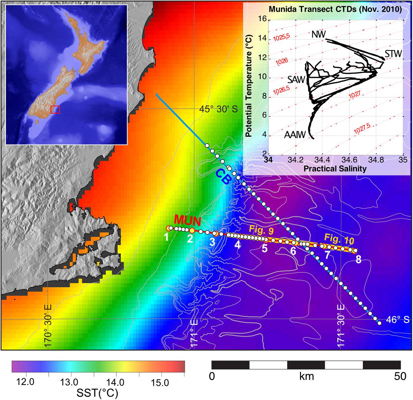
Figure 2. Location of the Munida (MUN) and Canterbury Basin (CB) transects. Seismic lines KAH1201-1, -2, and -3 were acquired along transect MUN, and line KAH1201-5 was acquired along transect CB. SST dataset (same as in Figure 1) is enlarged to highlight focus area of this manuscript in the vicinity of the Subtropical Front. XBT positions are indicated by white dots. Subsets of transects shown in Figures 9, 10 are highlighted. Inset in upper left shows a map including bathymetry in the region surrounding New Zealand. The area of the main figure is indicated by a red box. Land topography shading is derived from NASA’s SRTM data. Projection is UTM 59 South. Inset in upper right shows a temperature-salinity diagram based on eight conductivity-temperature-depth (CTD) profiles collected along the Munida transect in November 2010 (CTD cast locations are indicated by yellow dots in the main figure and are labeled 1–8). Red contours are potential density (in kg/m3). Water mass interpretations are labeled: NW, Neritic Water; STW, Subtropical Water; SAW, Subantarctic Water; AAIW, Antarctic Intermediate Water.
Seismic Data
Seismic line CB82-94 (Western Geophysical Company/Shell BP Todd Canterbury Services Ltd, 1982) was acquired in December 1982 aboard MV Western Odyssey using an array of 18 airguns with a total volume of 1220 in3 (20 L) at a depth of 6 m and a 120-channel 3,000 m long hydrophone array (25 m group spacing) towed at a depth of 11 m, with a near source-receiver offset of 168 m. The shot spacing was also 25 m resulting in a nominal fold of 60. A sample rate of 4 ms was used, with a record length of 6 s. Locational positioning was undertaken using microwave ranging to land-based stations.
The KAH1201 seismic data were acquired in January 2012 using a Sodera 45/105 in3 (0.74/1.72 L) GI (Generator-Injector) airgun operating at a depth of 5 m. A Geometrics GeoEel Digital Streamer was used, consisting of three active segments each 100 m long, with a total of 24 groups spaced at 12.5 m. Each group included 16 equally spaced hydrophone elements. The streamer was flown at a depth of 2.5 m, except on line KAH1201-2, where it was set to 4 m during bad weather. The depth of the streamer was controlled by a 5011 Digicourse bird at the head of each the three active segments. The near source-receiver offset was 30 m and the crossline offset between source and streamer was 8.2 m. The source was fired every 10.8 s with the vessel traveling at 4.5 kts, giving an average shot spacing of 25 m. Nominal fold is therefore 6. A sample rate of 1 ms was used, with a record length of 5 s. Satellite navigation was used for locational positioning.
The seismic data were processed using the GLOBE Claritas software package (Ravens, 2001). Details of the processing are described by Cooper (2021). For the KAH1201 data, the flow included 10/20 Hz high-pass filtering of the shot records and the application of a direct arrival filter by way of 5-trace median subtraction filtering after linear moveout at 1,498 m/s. The data were sorted into common-midpoint gathers, binned using the receiver group spacing (twice the natural midpoint spacing) to increase the nominal fold of the data from 6 to 12. Gain correction was applied using an automatic gain control (AGC) operator of 50 ms. Normal moveout correction was performed using velocities derived from the XBT data. Although “hand-picked” stacking velocities are often preferred in seismic processing (e.g., Fortin and Holbrook, 2009), the small source-receiver offsets of KAH1201 make the data unsuitable for semblance analysis, and relatively insensitive to small changes in NMO velocity, as discussed in more detail by Cooper (2021). Before stacking, a 15/30/150/180 Hz bandpass filter was applied, and channels 1, 9, and 17 were removed due to excess noise, possibly caused by the depth-control devices at the start of each of the three streamer segments. After stacking, a 25/40/150/180 Hz bandpass filter was applied and the data were muted below the seafloor. A poststack deconvolution was then applied, in the form of a zero-phase spectral whitening with a 5 Hz smoothing operator in the frequency domain. The data were migrated using a finite-difference time-domain algorithm with interval velocities calculated from the XBTs. A post-migration coherency filter was applied to remove random noise, consisting of a 5-trace weighted summation in the f-x domain. The 25/40/150/180 Hz bandpass filter and the seafloor mute were reapplied to remove noise created by the migration. A 45 ms taper was applied at the top of the section to remove migration artifacts created in the shallowest portion of the section where there is no signal due to the near offset. Finally, a static shift of 6 ms for line KAH1201-2 and 5 ms for the other lines was applied to account for the source and receiver depths.
Profile CB82-94 was processed using a similar flow. However, for these lower frequency data an AGC operator length of 100 ms was used and the bandpass filter was 2/15/100/120 Hz. The greater number of channels meant that a longer 11-trace filter was optimal for the direct arrival and coherency filtering. CDP binning was assigned using the same geometrical constraints and 12.5 m spacing as the KAH1201-5 profile to facilitate direct comparisons of the two datasets. Velocities used in the CB82-94 processing were determined using interactive semblance-based NMO velocity analysis every 50 CDPs.
Oceanographic Data
Oceanographic data were collected in the form of expendable bathythermographs (XBTs), providing measurements of temperature with depth at select locations along the seismic lines. Two types of XBTs were used: 40 Sippican Deep Blue XBTs for shallower seafloor depths and 40 Sippican T5 XBTs for deeper water. The XBTs were deployed at an average spacing of 1 nautical mile (∼1.85 km) along lines KAH1201-1 and KAH1201-5, with repeat measurements at select locations along KAH1201-2 and -3 (see Supplementary Tables 1, 2). Sound speed values were calculated using the Mackenzie (1981) equation; both RMS and interval velocities were calculated for use in seismic processing. Since the XBTs do not provide salinity data, a constant salinity of 34.4 was used in the Mackenzie equation, which is the average salinity from previous CTD profiles along the Munida transect (e.g., Figure 2). The sensitivity of seismic velocity to salinity is known to be relatively small (e.g., Sallarès et al., 2009) and tests on the CTD data show that the difference between velocities calculated using measured salinities compared to the constant salinity is no more than 0.04% (0.6 m/s).
Synthetic seismograms were calculated from the XBTs for use in comparing to the processed seismic data. Synthetic seismograms are a simulation of the seismic response of a given vertical distribution of density and seismic velocity (which are both functions of water temperature, salinity, and depth) to a particular source wavelet (e.g., Yilmaz, 2001). The synthetic seismograms were computed in MATLAB using functions in the CREWES toolbox (see Margrave and Lamoureux, 2019). The source wavelet used was modeled on a wavelet extracted from the processed seismic data; the extraction was performed in a window around a strong, isolated water-column reflection in the final image from line KAH1201-5.
Results
Seismic Images
Figure 3 shows the seismic images from lines KAH1201-1 and KAH1201-3 along the Munida Transect, and Figure 4 shows line KAH1201-5 along transect CB. The seismic images display strong reflectivity between 0.05 and 0.5 s; above 0.05 s (∼40 m) muting of the direct arrival has removed any data, and below 0.5 s (375 m) reflections are not visible over the noise level. Annotations show several reflective regions. In particular, strong reflections are visible at around 0.1 s (75 m) in the offshore region, sometimes in vertical stacks going down to 0.25 s (∼190 m) in isolated areas. Blank zones are present on the shelf and near the shelf break, and below the strong offshore reflections. Dipping reflections are visible near the shelf break, with dips of up to 3°. Above these shoreward-dipping reflections is a seaward-dipping reflection near the surface, especially in lines KAH1201-1 (Figure 3A) and KAH1201-5 (Figure 4), with a dip around 0.3°. Undulations are visible in most of the reflections, with the largest amplitudes in the shallow reflections in line KAH1201-3 (Figure 3B); these are interpreted to be internal waves, following similar interpretations in other seismic oceanography studies (e.g., Holbrook et al., 2003; Holbrook and Fer, 2005; Krahmann et al., 2008; Piété et al., 2013).
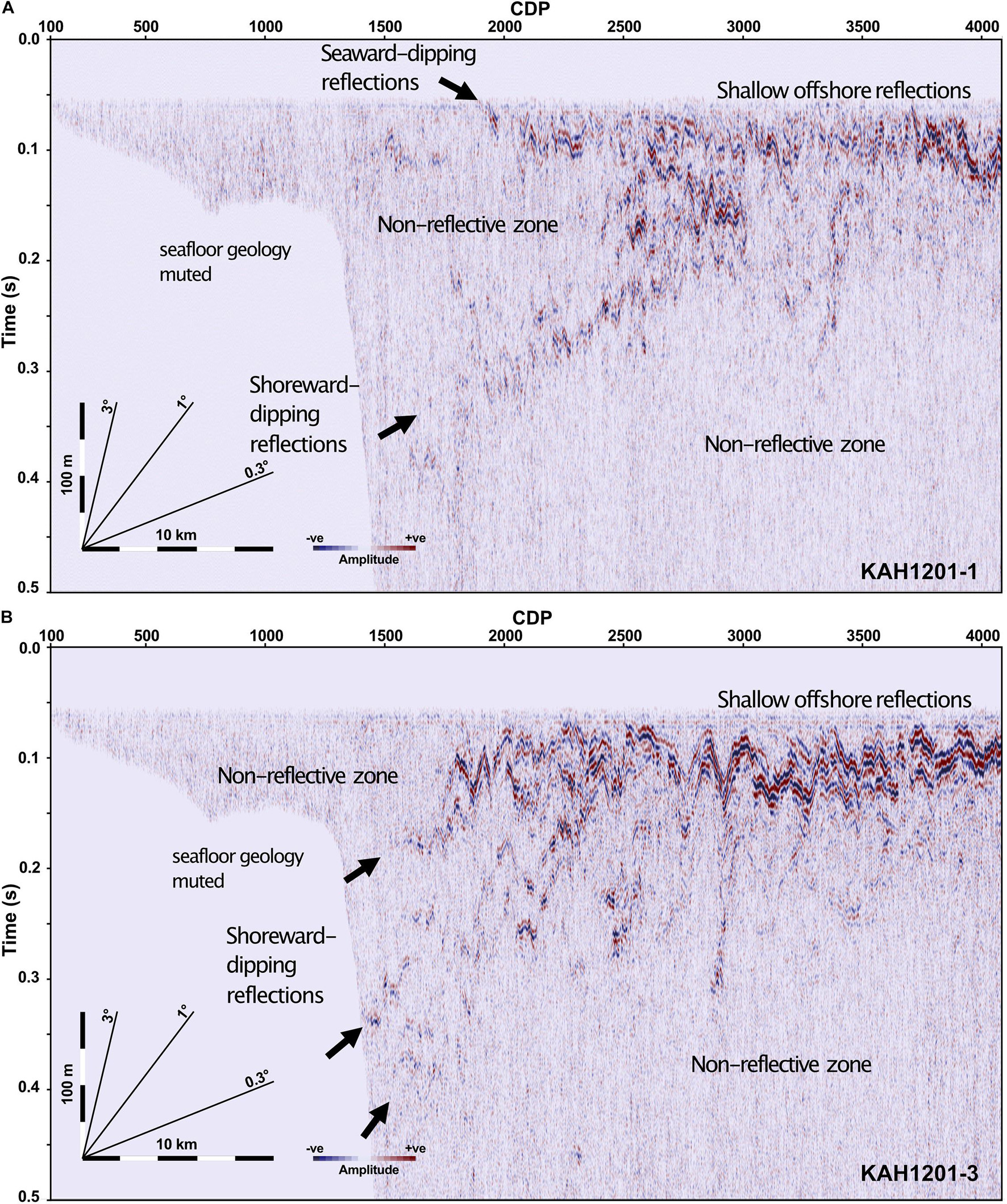
Figure 3. Processed seismic images for lines (A) KAH1201-1 and (B) KAH1201-3 from the MUN transect.
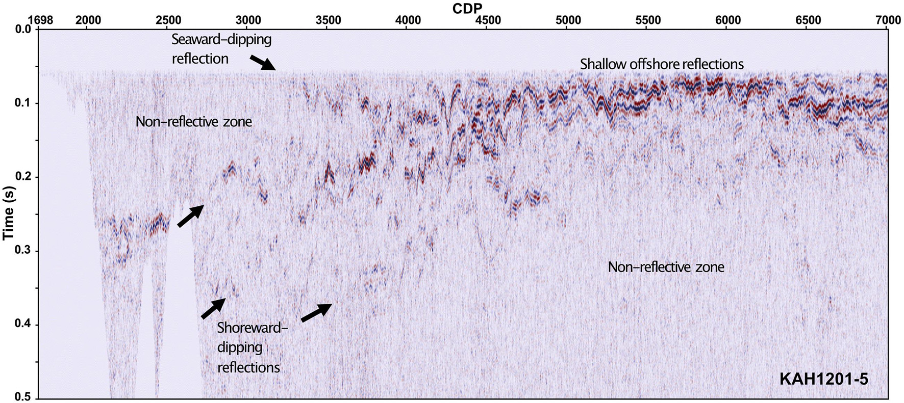
Figure 4. Processed seismic image for line KAH1201-5 from the CB transect.
Oceanographic Data and Synthetic Seismograms
The XBT section from KAH1201-1 is shown in Figure 5, with both temperature (A) and vertical temperature gradient (B) plotted. These data allow for the identification of the main water masses present, with warm (>∼11°C) STW on the shelf and near the shelf break, and cooler (<∼8°C) SAW further offshore. At depth, the two water masses are separated by a shoreward-dipping region of strong temperature gradients, indicated by the closely spaced isotherms approximately centered around the 9–9.5°C contours. This region is highlighted by the inclined dashed lines and represents the subsurface expression of the STF. The position of the STF can also be seen at the surface; the surface trace at the top of the section shows a ∼2°C temperature drop, with the approximate midpoint of this gradient region shown by an arrow. The surface trace was created by extracting the shallowest measured temperature from each XBT along the line. The satellite SST image in Figure 2 provides confirmation that this position corresponds to the location of the STF at the surface. In the offshore region, the SAW is overlain by a surface mixed layer with a sharp thermocline at its base. Small areas of temperature inversions can be seen in the middle of the section, particularly on the 9 and 10°C contours.
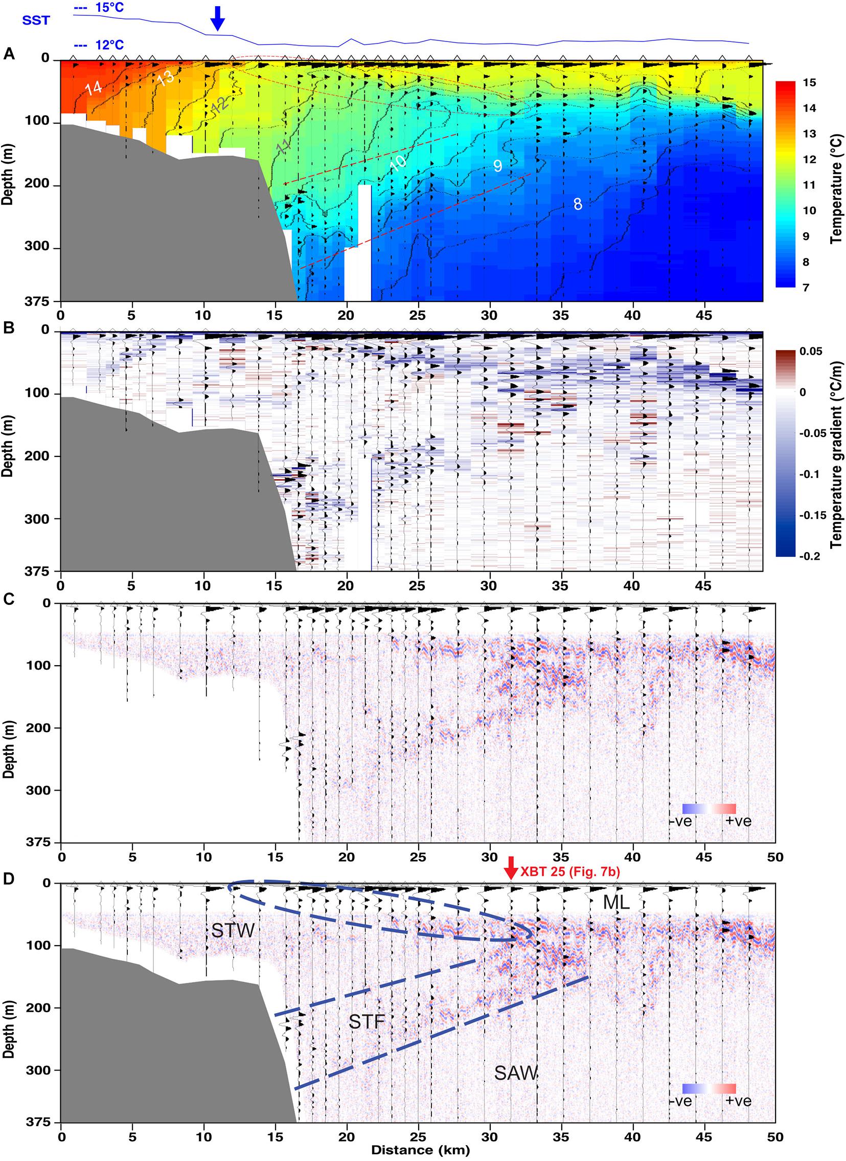
Figure 5. (A) Temperature, (B) vertical temperature gradient, (C) uninterpreted seismic image, and (D) interpreted seismic image for line KAH1201-1, with synthetic seismograms overlain on each image. Shoreward- and seaward-dipping reflective zones separating interpreted water masses are highlighted by dashed lines. STW, Subtropical Water; STF, Subtropical Front; SAW, Subantarctic Water; ML, mixed layer. The surface temperature trace, with approximate surface STF location indicated with an arrow, is shown at the top of (A). Arrow in (D) indicates the location of XBT shown in Figure 7.
Figure 5 also shows the synthetic seismograms for line KAH1201-1 overlain on both the XBT and seismic data. The synthetic traces help identify which oceanographic features are expected to be imaged in the seismic data, specifically what the different water masses will look like and what boundaries should be visible. One strong, continuous seismic response is associated with large temperature gradients at the base of the mixed layer (at depths of ∼50–100 m), present in offshore regions (over kms 30–50). Another region of high reflectivity is present in the shoreward-dipping zone of high temperature gradients separating STW and SAW that intersects the shelf break at depths between ∼200 and 400 m; this extends out to approximately the 30 km mark and represents the subsurface STF. Line KAH1201-1 also shows a seaward-dipping reflective region at shallow depths (0–50 m) in the middle of the section (kms 15–30), approaching the surface near the surface location of the STF; this region is highlighted by a dashed oval. The seaward- and shoreward-dipping reflective zones trace the outline of a warm-water “wedge” extending seaward from the shelf break. The synthetic seismograms show that the warm STW “wedge” region is largely non-reflective. However, an additional shoreward-dipping reflection is present on the shelf (kms 2–7), particularly visible in the gradient section, which could be a neritic front separating warm, salty STW from inshore warm, fresher neritic water. On the seaward side of the STF, the region beneath the mixed layer occupied by cool SAW is also a zone of low reflectivity.
The XBT section from line KAH1201-5 (Figure 6) shows a similar pattern to line KAH1201-1. Temperatures are slightly higher in the warm-water wedge, with the 11.5–12°C contour region occupying a greater area, whereas the 10.5–11°C contour region was larger in KAH1201-1. The surface temperature drop occurs over a longer distance than in line KAH1201-1 (over kms 66–50 compared to kms 7–14), but this is partly expected due to the more oblique angle of the line as seen in Figure 2). The midpoint of this gradient region is taken to represent the surface position of the STF, and is indicated in Figure 6 by an arrow. One feature that is present in line KAH1201-5 is a minimum in surface temperatures in the middle of the section (kms 50–30), with warmer surface temperatures both inshore and offshore; this feature is seen to a lesser degree in line KAH1201-1. Temperature inversions are again visible, in the 8–12°C contours.
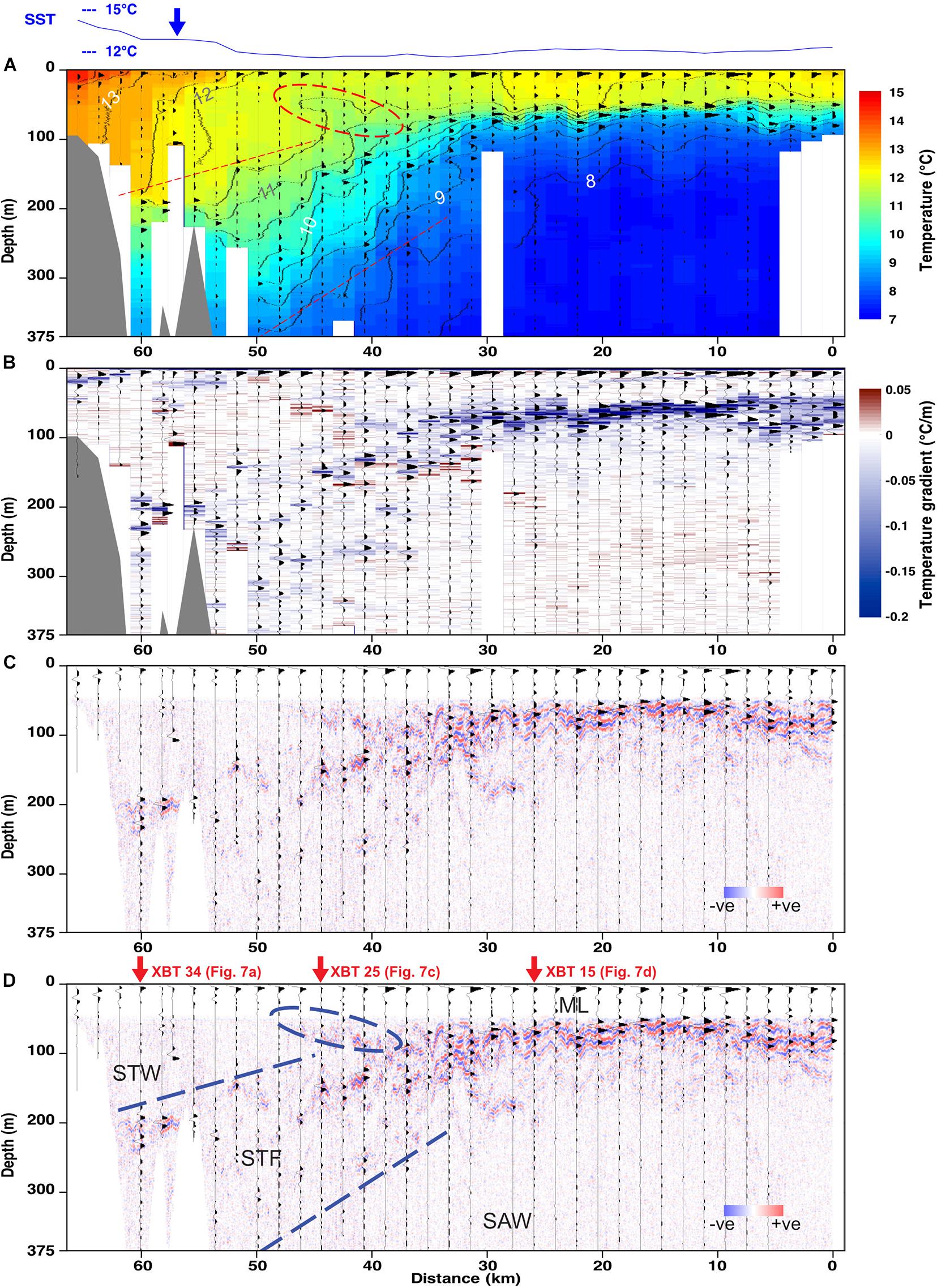
Figure 6. (A) Temperature, (B) vertical temperature gradient, (C) uninterpreted seismic image, and (D) interpreted seismic image for line KAH1201-5, with synthetic seismograms overlain on each image. Shoreward- and seaward-dipping reflective zones separating interpreted water masses are highlighted by dashed lines. STW, Subtropical Water; STF, Subtropical Front; SAW, Subantarctic Water; ML, mixed layer. The surface temperature trace, with approximate surface STF location indicated with an arrow, is shown at the top of (A). Arrows in (D) indicate the location of XBTs shown in Figure 7.
Synthetic seismograms overlain on the XBT and seismic data in Figure 6 again show three main zones of high reflectivity. These are associated with the high temperature gradients at the base of the mixed layer (depths of ∼50–100 m between kms 30–0), the enhanced gradients of the STF in a shoreward-dipping zone intersecting the continental slope (outlined by dashed lines), and a smaller shallow seaward-dipping zone associated with temperature inversions (dashed oval outline). Two zones of low reflectivity are also present, corresponding to warm STW inshore of the STF and cool SAW seaward of the STF and beneath the mixed layer.
The temperature cross-sections in Figures 5, 6 show a significant difference between the surface and subsurface expressions of the STF. In both lines the subsurface expression of the STF, seen as the dipping region of enhanced temperature gradients separating the warmer STW from cooler SAW, extends much further offshore (by up to ∼25 km) than the surface location of the STF as seen in the surface traces. The XBT data show the surface expression on the shelf or near the shelf break, while the subsurface expression (seen in both the XBT and seismic data) is a broader region extending much further offshore. The strong mixed layer overprints the subsurface expression of the front in the offshore region, which means that it is not visible in the surface temperature data, including satellite SST.
Seismic Interpretations
General comparisons between the synthetic seismograms and seismic images in Figures 5, 6 allow for the matching of oceanographic features identified in the XBT sections, including Subtropical and Subantarctic water masses, the Subtropical Front, and the base of the offshore mixed layer, to their corresponding expressions in the KAH1201 seismic images. These oceanographic features have been observed with similar distributions in many previous CTD transects in the region (e.g., Jillett, 1969; Sutton, 2003; Jones et al., 2013), as well as in nearby legacy seismic data (e.g., Gorman et al., 2018; Cooper, 2021), but the coincident acquisition of oceanographic and seismic data in this study allow for specific reflections to be examined in more detail, giving more insight into their oceanographic origins; this is accomplished by way of individual synthetic ties such as those shown in Figure 7.
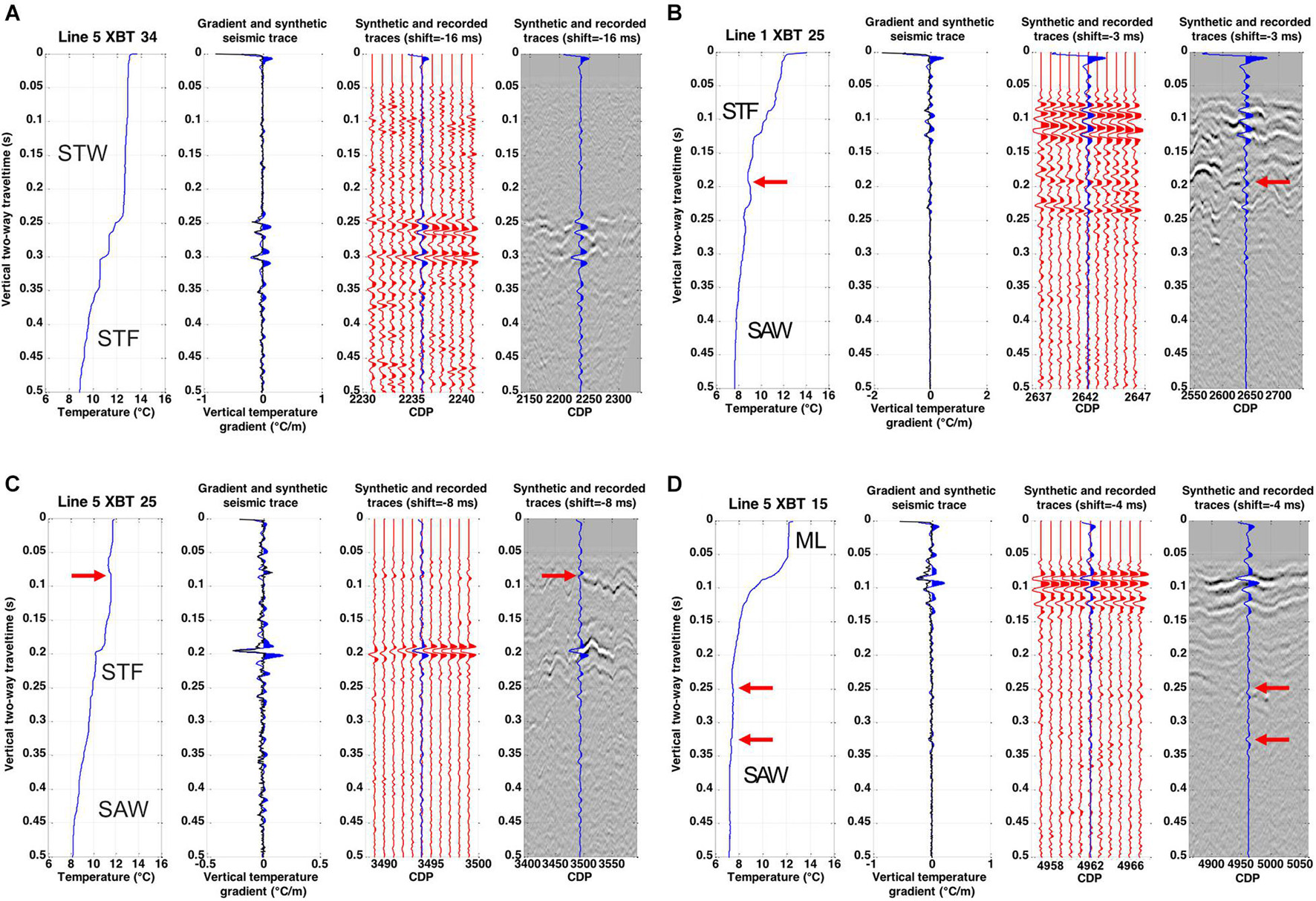
Figure 7. Synthetic seismic ties for XBTs showing STW (A), the STF (A–C), SAW (B–D), and the mixed layer (ML) (D). Each of (A–D) consists of four panels, from left to right: temperature as a function of seismic travel time, vertical temperature gradient (black) and the synthetic seismic trace (blue), the synthetic seismic trace (blue) overlain on 11 adjacent traces from the recorded seismic data (red wiggle traces), and the synthetic seismic trace (blue) overlain on 201 adjacent traces from the recorded seismic data (greyscale image). Red arrows in (B,C) indicate temperature inversions associated with positive-polarity reflections. Arrows in d indicate weak reflections within SAW.
Figures 5, 6 previously showed a large non-reflective zone associated with warm temperatures in the shallow, inshore portion of the seismic images, corresponding to STW. Reflections are visible at the base of this zone near the shelf break, and in particular on line KAH1201-5 where canyons cut through the shelf. Figure 7A shows a synthetic tie for this region, confirming the non-reflective nature of the shallow STW above the STF.
In Figures 5, 6 the STF manifests as dipping reflections associated with high temperature gradients in the subsurface, with warm non-reflective STW above, cool weakly reflective SAW below, and temperatures suggesting a mixture of the two water masses in between. Figure 7 shows several synthetic ties in this region, with distinct negative-polarity reflections where the temperature gradient contains sharp steps over a range of depths (in A and C), creating a stack of interfering reflections where the isotherms come together at the tip of the warm-water wedge (B). The STF region also shows examples of temperature inversions and associated positive-polarity reflections; an example is highlighted in Figure 7B. The seismic peaks associated with temperature inversions in the STF region are not particularly continuous laterally in the full seismic images, suggesting perhaps that these features are not stable.
One positive-polarity reflection that is laterally continuous is the seaward-dipping reflection identified earlier in the shallow region overlying the warm-water wedge. Figure 7C shows a synthetic tie for this feature. At 0.08 s (∼60 m) there is a temperature inversion, with temperatures near 12°C above and below, and a small region of cooler 11.5°C water in between, and a positive-polarity reflection is present. This feature is interpreted to represent the boundary between warm, shallow SAW present in the mixed layer offshore and warm STW or STW/SAW mix present on the shelf and in the subsurface warm-water wedge. While the temperature difference between the warm SAW mixed layer and the warm subsurface STW is small, the salinity difference between these two water types is large, as seen in previous CTD data in this region (e.g., Figure 2), meaning that subsurface salinity data would show this boundary more clearly than the XBT sections.
Further offshore, Figures 5, 6 show a shallow high-reflectivity zone associated with the mixed layer, separated by a strong thermocline from underlying SAW. Figure 7D shows a synthetic tie for this region. The mixing history of the near-surface layer is preserved in the character of the mixed layer reflections; multiple, stacked reflections represent different mixing events causing discontinuities in the overall temperature gradient. Beneath the mixed-layer reflections, the SAW is non- or weakly reflective; reflections in this zone are associated with small temperature fluctuations indicating slight heterogeneity in the SAW. The weakly reflective nature of the SAW is consistent with observations in previous legacy seismic investigations in the study area (Smillie, 2012; Gorman et al., 2018; Cooper, 2021). Particularly non-reflective zones may be associated with very homogeneous near 7°C Subantarctic Mode Water, which is known to be present in the region (e.g., McCartney, 1977; Morris et al., 2001; Chiswell et al., 2015).
Discussion
Comparison to Legacy Seismic Data
Because KAH1201-5 and the legacy industry seismic line CB82-94 are co-located, the main features identified in KAH1201-5 can be traced to CB82-94. Figure 8 shows both lines on the same scale. The major differences in water-column imaging between the lines are a result of the vastly different acquisition parameters, with CB82-94 acquired using a large low-frequency airgun array compared to the small single G/I gun of KAH1201-5, and a longer streamer containing many more receivers (3 km and 120 channels vs. 300 m and 24 channels). The resulting differences include the higher frequency content of line KAH1201-5; a comparison of the amplitude spectra of the data gives a dominant frequency of 70 Hz in KAH1201-5 and 20 Hz in CB82-94, indicating that the KAH1201 data can image layers that are less than a third of the thickness of those observed by the legacy seismic set-up. The smaller near offset in the source-streamer geometry of KAH1201 results in more detail at shallow depths, especially with the seaward-dipping reflection connecting the surface and subsurface expressions of the front, but the lower energy of the source and lower fold result in greatly reduced reflectivity observed in the deeper portion of the water column. The CB82-94 line has a larger gap in the shallow part of the image (∼60 m vs. 40 m) due to direct-arrival interference and muting, but shows significant reflectivity at greater depths; the synthetic seismograms suggest that this is the transition between SAW and underlying Antarctic Intermediate Water (AAIW), expected at depths between 500 and 1,000 m, and therefore not imaged in the KAH1201 data. The deep, non-reflective AAIW and a possible lens or eddy-like feature at the end of the line between CDPs 6400 and 6800 are also present in the CB82-94 image. Since the eddy feature is centered near 0.5 s (375 m) in the legacy data and the KAH1201 data show no reflectivity below 0.5 s it is possible that similar features may be present in the KAH1201 data but are not (or only partially) imaged.
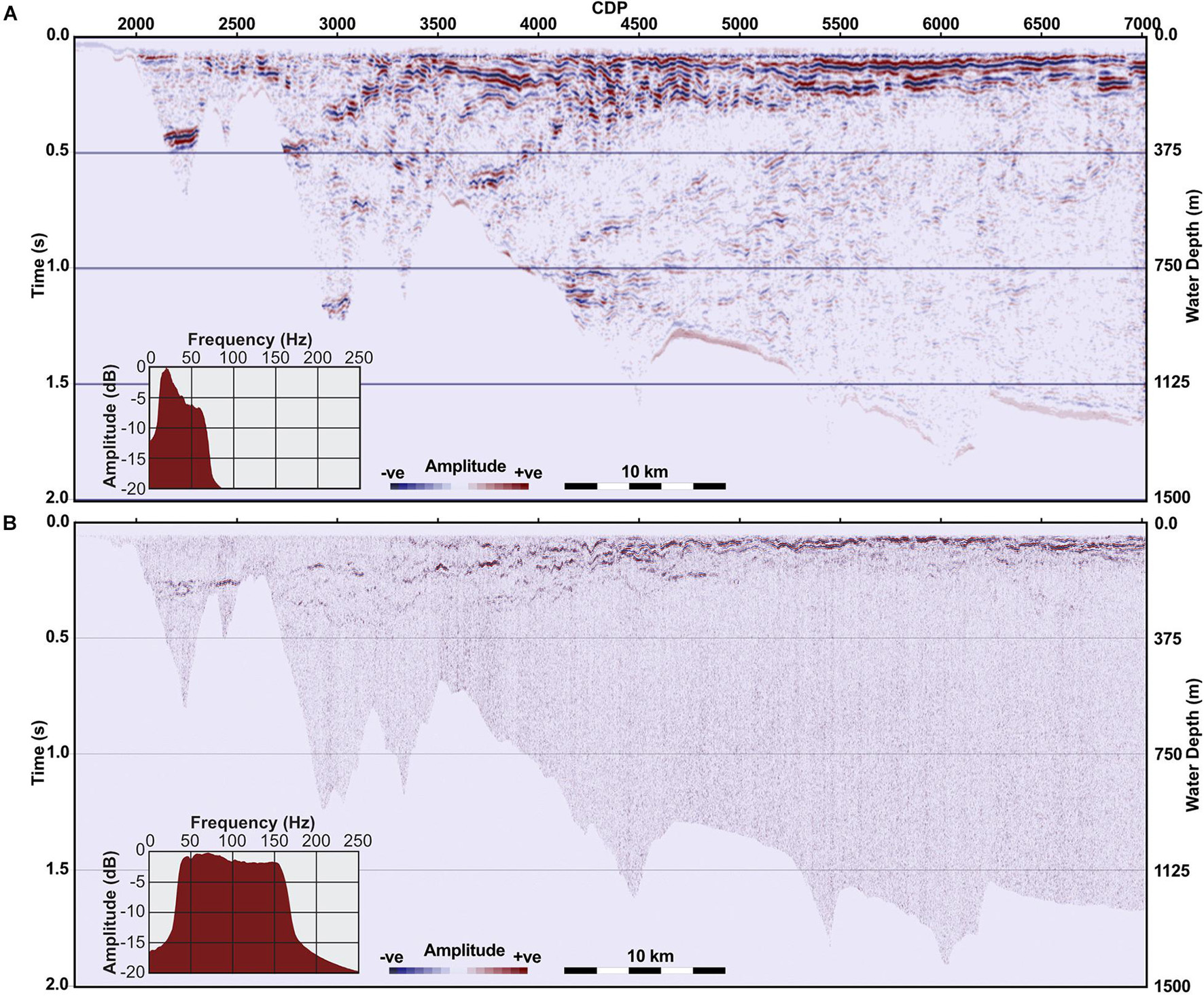
Figure 8. Seismic data from the CB transect, showing comparison between (A) industry line CB82-94 collected in 1982 and (B) line KAH1201-5. Amplitude spectra calculated from water column reflectivity show the difference in frequency content of the two datasets.
At shallow depths, the two seismic lines show many similarities in their reflectivity pattern, but also some strong differences. Similarities include the reflections in the canyons just off the shelf break, the strong shallow reflections offshore, and the shoreward-dipping reflections. These are consistent with the base of the STW, the base of the mixed layer, and the subsurface expression of the STF. The features are not identical, however, as expected due to the 29-year time gap between the acquisition of the images. Seasonally, the two lines are similar, with CB82-94 acquired in late December, compared to the late January KAH1201 cruise. Observable differences include the canyon reflection (at CDPs 2000–2500) that is deeper by about 0.2 s (∼150 m) in CB82-94 and dipping reflections (CDPs 2700–3250 and 3600–4200) that are deeper by a similar amount and approximately twice as steep (∼2°) in CB82-94, perhaps indicating a stronger front and current at that time. The non-reflective STW does not appear to extend as far offshore in CB82-94 (ending near CDP 3200 vs. 3800 in KAH1201-5, a difference of ∼5 km), and the reflective region outlining the warm-water wedge extends further offshore (CDP 4800 vs. 4600, ∼2.5 km). The mixed layer region at CDPs > 5250 in the CB82-94 image is composed of two strong continuous reflections extending to ∼0.24 s (∼180 m), as opposed to the mostly solitary, shallower (∼0.05–0.16 s or 40–120 m) mixed layer reflection in the KAH1201-5 image.
Time-Lapse Comparisons
Time-lapse changes can be observed by comparing lines KAH1201-1, 2, and -3, all acquired along the Munida Transect, with lines 1 and 2 acquired continuously, followed by a gap of 11 h and 20 min before the start of line 3. Line KAH1201-2 was aborted early so only the offshore portion of the Munida Transect was imaged, while both KAH1201-1 and -3 imaged the entire transect. Initial comparisons of the lines made previously (Figure 3) showed overall similarities, but also significant changes in the mixed-layer reflection and associated internal waves, as well as in the reflections associated with the STF. In particular, the difference between lines 1 and 3 is striking, given their identical location and short time between acquisition. Figure 9 shows in more detail the difference in the STF reflections in lines KAH1201- and -3, with XBT temperatures overlain. The bulk of the shoreward-dipping reflective zone moved shoreward from line 1 to line 3 (approximately from CDP 3000 to 2400, or 7.5 km), but the XBTs show that warm STW (indicated by the blank zone with red temperatures and the reflection at its base) moved further seaward (∼from CDP 1500 to 1700, or 2.5 km). This is similar to the change observed between lines KAH1201-5 and CB82-94: in line CB82-94 the STW did not extend as far offshore, but the zone of dipping STF reflections extended further offshore than in line 5. If the motion of the STF (as represented by the dipping reflections) was confined to the plane of the section, movement of ∼7.5 km in the ∼19 h elapsed between lines KAH1201-1 and -3 would suggest a minimum velocity of ∼0.1 m/s. However, some of the apparent variability in the STF reflections is likely spatial in origin. Satellite sea-surface temperature images of this region indicate a high degree of meandering in the front toward and away from shore (e.g., Figure 2; Shaw and Vennell, 2001). These meanders would be carried within the overall flow of the northeastward-flowing Southland Current and pass through the position of the seismic line, causing apparent along-section movement of the water mass boundaries and associated reflections.
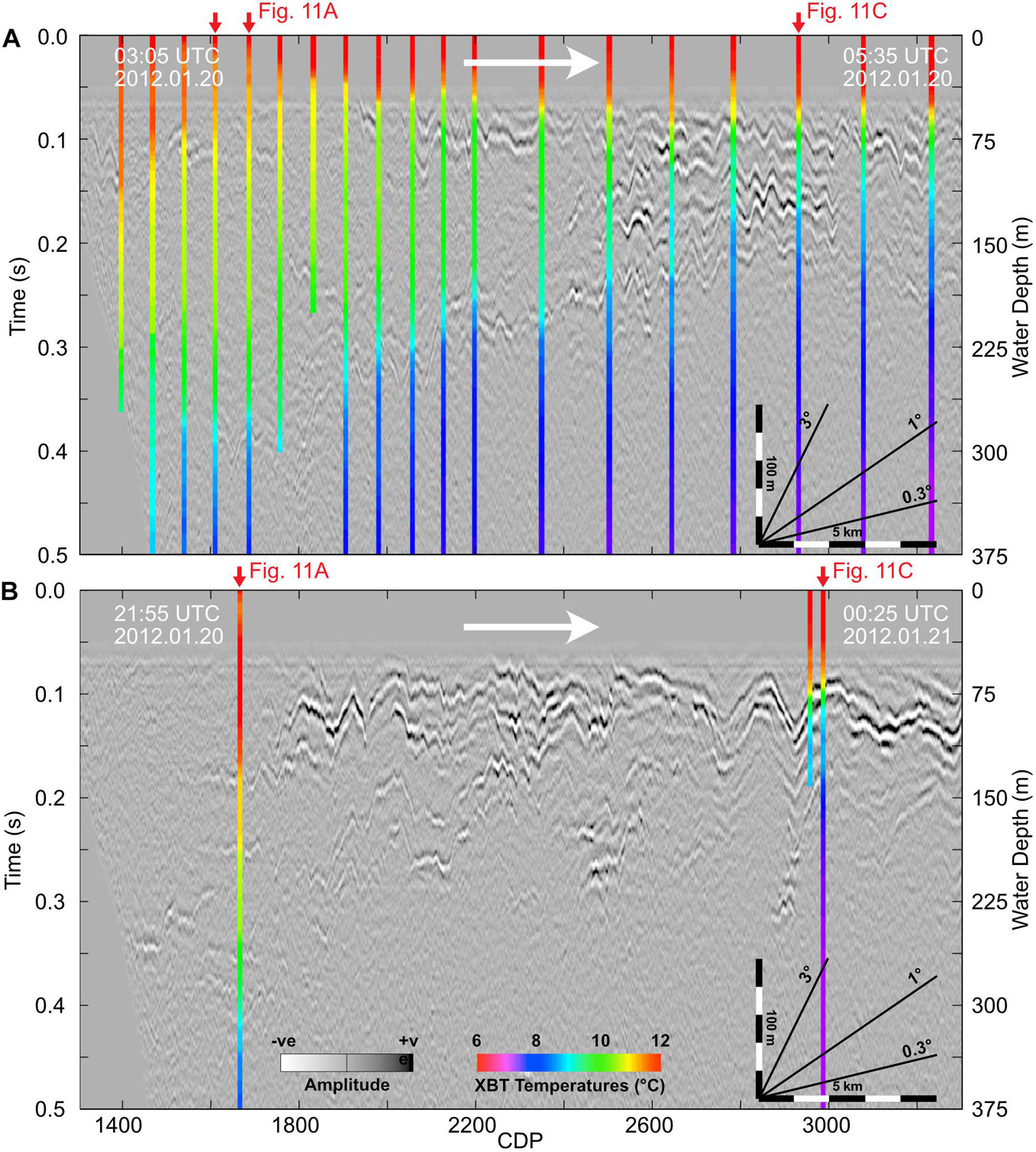
Figure 9. Portions of lines KAH1201-1 (A) and KAH1201-3 (B) acquired in the same location (as indicated in Figure 2), with acquisition times and directions indicated by white arrows. Differences in STF reflections (cf. Figure 5D) can be observed. XBT temperatures are overlain in color. Red arrows indicate the location of XBTs shown in Figure 11.
Time-lapse changes can also be observed in the seismic images from the seaward end of the Munida Transect. Figure 10 shows the equivalent portions of lines KAH1201-1, -2, and -3. Lines 1 and 2 were acquired consecutively, so the extreme right-hand side of both images is nearly identical with only a 10-min delay as the ship turned, but the differences in the rest of the image are large, with individual reflections not able to be correlated between the two images. Despite that, the character of the two images is similar, especially when compared to line KAH1201-3. Line 3 contains strong, continuous stacks of reflections, with long-wavelength perturbations, whereas lines 1 and 2 contain reflections that are weaker and less laterally continuous, with shorter wavelength internal waves. The difference could be due to the surface weather conditions, with strong winds causing the termination of line 2 and the nearly 12-h time delay before the start of acquisition of line 3, potentially resulting in mixing of the surface layer and the development of a new, sharper and more continuous thermocline. Some of the difference could also be because of weather-induced data quality deterioration causing reflections to appear weaker and less continuous in lines 1 and 2.
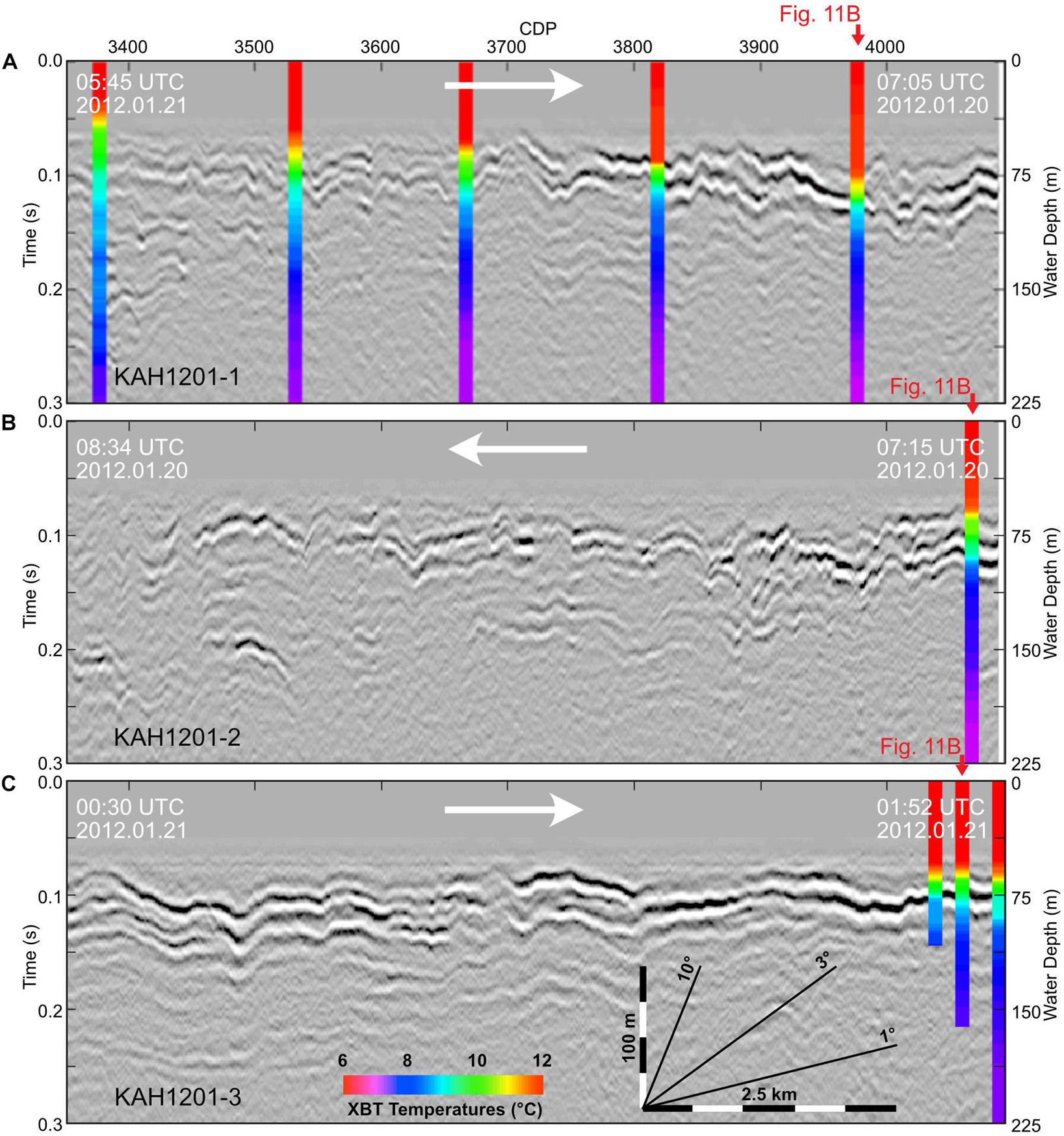
Figure 10. Portions of lines KAH1201-1 (A), KAH1201-2 (B), and KAH1201-3 (C) acquired in the same location (as indicated in Figure 2), with acquisition times and directions indicated by white arrows. XBT temperatures are overlain in color. Red arrows indicate the location of XBTs shown in Figure 11.
During the seismic acquisition, XBTs were repeated at different locations, which provide more insight into the differences observed in the seismic data from repeat passes. Figure 11A shows three XBTs taken along the Munida Transect at approximately the same location within the STF region (indicated by the arrows in Figure 9), occupied during lines KAH1201-1 and -3. The two XBTs on line 1 were acquired 6 min apart, and show great similarity in the temperature profile, as well as similarity in the seismic character laterally between the two locations. The XBT on line 3, 19 h later, shows much warmer temperatures over most of the depth range displayed, and more steps in the temperature profile compared to the smoother gradient on line 1. As a result, the seismic section displays a greater number of reflections in the middle of the image. As noted previously, this change is very striking as it occurred over such a short time period and demonstrates the highly dynamic nature of the STF in this region. A change of 1°C in temperature at the same location in less than 24 h suggests significant meandering of the front spatially, at least at depth; unfortunately, a surface temperature trace was not available for line 3 to compare the surface position of the STF between the two lines.
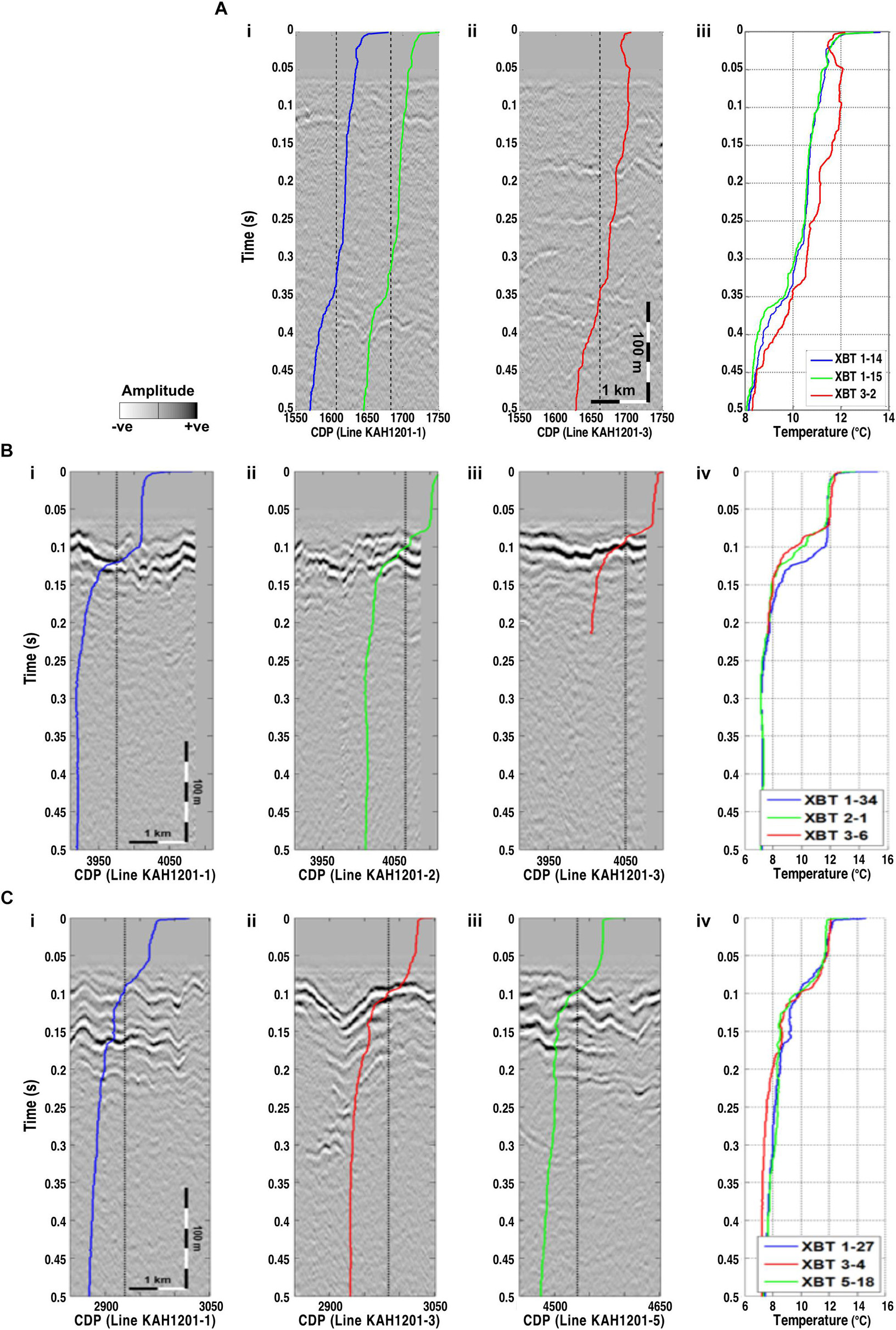
Figure 11. Time-lapse XBT comparisons. Temperature traces are overlain on the seismic data, with the XBT locations shown by vertical dotted lines. (A) Portions of lines KAH1201-1 (i) and KAH1201-3 (ii) acquired in the same location within the STF zone. The three XBTs are plotted together in (iii). The time delay between XBTs 1-14 and 1-15 was 6 min, and between 1-15 and 3-2 was 19 h. (B) Portions of lines KAH1201-1 (i), KAH1201-2 (ii), and KAH1201-3 (iii) acquired in the same location at the seaward end of the Munida Transect. The three XBTs are plotted together in (iv). The time delay between XBTs 1-34 and 2-1 was 25 min, and between 2-1 and 3-6 was 18.5 h. (C) Portions of lines KAH1201-1 (i), KAH1201-3 (ii), and KAH1201-5 (iii) acquired at the intersection point of transects MUN and CB. The three XBTs are plotted together in (iv). The time delay between XBTs 1-27 and 3-4 was 19 h, and between XBTs 3-4 and 5-18 was 8 h.
The XBTs from the seaward ends of the lines in Figure 10 are displayed in Figure 11B. The two XBTs from line 1 and 2 were acquired 25 min apart, and the XBT from line 3 was acquired 18.5 h later. The three temperature profiles are nearly identical in the mixed layer and below the thermocline. The XBTs from lines 2 and 3 are most similar, despite the larger time delay, suggesting that spatial differences are the greater factor when considering changes in the base of the mixed layer, rather than time lapse changes over these time scales. This is also evident by the significant lateral changes in the mixed-layer reflections seen in the seismic sections. Internal waves displacing the mixed-layer reflections are also likely to contribute to the time-lapse changes.
The last location sampled with XBTs repeatedly was the intersection point between transects MUN and CB. The location was visited three times, during the recording of lines KAH1201-1, -3, and -5 (Figure 11C). Its position is indicated on Figure 9 for the MUN lines; it corresponds to km 31 on line KAH1201-5 (Figure 6). The three temperature profiles again show differences in the thermocline at the base of mixed layer, with line 1 showing a deep strong reflection with weaker shallow reflections, line 3 showing a shallow strong reflection, and line 5 showing several moderate reflections. The XBT from line 3 differs from the other two profiles at depth, with cooler temperatures measured below 0.18 s (∼135 m). The previous comparison of lines 1 and 3 noted that the dipping STF reflections and associated high temperature-gradient region moved shoreward between the two lines; the process appears to have been reversed by the time of the acquisition of line 5. Another possibility is that the temperature difference at depth in line 3 is related to a possible eddy suggested by the “V”-shaped feature seen in the mixed-layer reflection to the left of the XBT location. Though this XBT just misses the stack of reflections extending downwards from the “V” to 0.31 s, it may be showing the effect of the feature. Either way, the changes in the seismic images and temperature profiles are evidence for a highly variable front over short timescales (on the order of hours).
Methodological Impact
The results of cruise KAH1201 demonstrate that cost-effective research-scale experiments can be used for dedicated seismic oceanography research examining shallow (e.g., < 400 m water depth) oceanographic features. The cruise yielded reasonable quality, high-frequency seismic data, with coincident oceanographic data. This cruise was the first time that unambiguous water-column reflections were visible in a dedicated seismic oceanography voyage in this area. The seismic images have much greater horizontal resolution than the coincident XBT sections alone and even higher resolution than previous CTD sections along the 8-station Munida Transect. Although poor weather adversely affected the amount of seismic data collected during this cruise, one seismic profile was able to be repeated during the cruise to examine time-lapse changes in the reflectivity—importantly with repeat oceanographic data as well.
The KAH1201 survey resulted in good-quality high-frequency seismic images with significantly more detail in the shallow portion of the water column (<150 m) compared to legacy seismic data (Figure 8). Although the legacy data have a higher signal-to-noise ratio and contain reflections in the deeper portion of the water column which are not seen in the KAH1201 images, smaller and shallower layers are able to be resolved in the new data, including the seaward-dipping portion of the STF connecting its surface and subsurface expressions. One disadvantage of the shorter hydrophone streamer in the KAH1201 survey is that it did not produce long enough source-receiver offsets for stacking velocity analysis to help with identifying water masses, which would be useful in situations where coincident oceanographic data are not available. On the other hand, the small source-receiver offsets mean that detailed (and potentially time-consuming) interactive velocity analysis is not needed for these types of surveys, in contrast to long-offset data (e.g., Fortin and Holbrook, 2009); for the KAH1201 data, even using a constant velocity for stacking produced virtually identical stacks to using XBT-derived velocities (Cooper, 2021).
As mentioned previously, when creating the final seismic images for the KAH1201 data, an AGC operator was applied. Compared to other gain correction methods such as spherical divergence, AGC can cause distortion of the relative amplitudes of seismic reflections. A more rigorous amplitude-preserving flow would be required for further analysis of this dataset (e.g., for the application of seismic inversion). However, for these shallow seismic data with high levels of background noise, a simpler processing flow was sufficient for producing images of the main water masses and boundaries, and comparisons with synthetic seismograms show that relative amplitudes were adequately preserved (e.g., Figure 7).
This survey adds to a growing body of work using similar methods to study a range of oceanographic problems. The frequency content of the new seismic data compares favorably to other high-frequency seismic oceanography studies (e.g., Hobbs et al., 2009; Carniel et al., 2012; Piété et al., 2013). The acquisition of repeat seismic lines along the same transect to examine time lapse changes has similarities to the investigations of Tsuji et al. (2005), Nakamura et al. (2006), Géli et al. (2009), and Gunn et al. (2020). Expendable bathythermographs were used to acquire oceanographic data, in a manner similar to other single-vessel seismic oceanography cruises (e.g., Nandi et al., 2004; Nakamura et al., 2006).
The XBTs provide corroboration of the oceanographic features observed in the seismic images. In particular, the data illustrate the presence of STW, SAW, and a mixing zone between the two, and a well-developed mixed layer offshore. Surface traces constructed from the XBTs were also tied to satellite sea-surface temperatures, which was important in comparing the surface and subsurface expressions of the Subtropical Front.
Synthetic seismograms confirmed that prominent reflections originate from the base of the mixed layer and from the Subtropical Front in the subsurface, seen as high temperature gradient regions. Overall, similar reflective features are observed in both the KAH1201 and CB82-94 data, which provides confidence in the interpretation of significant oceanographic features in legacy seismic data that typically lack coincident oceanographic data. This provides support for previous interpretations of water column features (e.g., Gorman et al., 2018), and also for interpretation of further legacy seismic data in the same framework. The reflections associated with the Subtropical Front show, in particular, that the subsurface expression of the front is much more complex than suggested by its surface expression, consisting of a highly variable zone of mixing including temperature inversions. This illustrates the value of seismic oceanography in this region, as the seismic data have a horizontal resolution that cannot practically be achieved using CTDs or XBTs; even with the dense XBT deployment used in this survey, the seismic images still represent over 100 times greater spatial sampling than the XBT sections, with a 12.5 m trace spacing compared to the ∼1.85 km XBT spacing.
Another first for this survey was the acquisition of time-lapse seismic data over the Subtropical Front. Although earlier work (Smillie, 2012; Gorman et al., 2018) examined nearby legacy seismic surveys that were acquired 2 years apart, this survey involved the acquisition of short-turnaround time-lapse images of the identical transect. Time-lapse changes in reflections were significant over small timescales. There were large changes in the mixed-layer reflections and the internal waves affecting the base of the mixed layer, even on the scale of minutes as seen in changes between lines KAH1201-1 and -2. There were also significant changes in the reflections associated with the STF over the scale of hours, as seen in changes between lines KAH1201-1 and -3. In general, the seismic data show that features and patterns are consistent between datasets, which allows for confidence in interpreting future data without acquiring large amounts of coincident oceanographic data. However, the time-lapse passes show that for detailed analysis, as opposed to general interpretations, the acquisition of significant oceanographic data on each repeat pass is needed at this stage to deepen our understanding of the reflective changes in the seismic data.
Importantly, this survey helps to constrain the minimum requirements for a successful seismic oceanography cruise studying features like the STF in New Zealand waters. This cruise tested a relatively affordable research-scale operation, using a vessel and acquisition system (45/105 in3 (0.74/1.72 L) GI gun and 300 m streamer) much smaller in scale than those of an industry seismic survey, that resulted in satisfactory seismic data and adequate accompanying oceanographic data, even in poor weather conditions. In fact, this cruise was smaller-scale in terms of seismic acquisition parameters (source size, streamer length, or both) than other “high-frequency” or “high-resolution” surveys of Géli et al. (2009) and Hobbs et al. (2009), and the GI gun surveys of Nakamura et al. (2006); Carniel et al. (2012), Piété et al. (2013), and Sarkar et al. (2015). This means that, apart from the Piété et al. (2013) sparker data where only the mixed layer is imaged, this cruise represents new minimum requirements for successful seismic oceanography acquisition.
Frontal Structure and Dynamics
The reflective region representing the STF in the KAH1201 seismic data is similar to other seismic oceanography studies of frontal zones which show enhanced seismic reflectivity and dipping reflections associated with thermohaline intrusions and interleaving, such as the work of Holbrook et al. (2003); Mirshak et al. (2010), Sheen et al. (2012), and Rice et al. (2014). Synthetic ties between the XBTs and recorded seismic data show individual reflections resulting from step-like changes in temperature as well as inversions within the overall zone of high temperature gradients. Inversions such as these are a known feature of the STF, both in temperature and salinity (e.g., Garner, 1967; Heath, 1975; Gilmour and Cole, 1979; Harris et al., 1993).
In addition to the zone of shoreward-dipping reflections, the high-frequency seismic images also show the presence of an overlying shallow seaward-dipping reflection connecting the tip of the reflective warm-water wedge to the surface at a position further inshore. This inshore position appears to correspond to the surface position of the STF as seen in surface temperature traces and satellite sea-surface temperature images. In this study the surface STF position is found near the shelf break, consistent with previous satellite SST studies. The surface temperatures also show a consistent pattern with the lowest surface temperatures immediately seaward of the surface STF position, overlying the subsurface STF reflective region, and slightly warmer waters offshore. These low surface temperatures have been previously identified as a cold “tongue” created by upwelling associated with the flow of the Southland Current (e.g., Burling, 1961; Hawke, 1989; Shaw, 1998; Hopkins et al., 2010). The association of the low-temperature zone with the Southland Current supports the interpretation of the high-reflectivity zone in the subsurface as representing the mixed STW and SAW in the core of the Southland Current.
In this study the subsurface zone of high reflectivity in the seismic images consistently extends further seaward than the surface position of the STF, by a distance of ∼25 km. The difference between the surface and subsurface expressions of the STF has been observed in previous studies using SST and CTDs. While the surface and subsurface positions of the STF are strongly linked (e.g., Smith et al., 2013), the surface expression of the STF, particularly with respect to temperature, can be disrupted, decoupled, or even erased (e.g., Burling, 1961; Ridgway, 1975; Jeffrey, 1986; Butler et al., 1992; Szymanska and Tomczak, 1994; Chiswell, 1996; James et al., 2002; Tomczak et al., 2004). The effect changes seasonally, with the front more plainly visible at the surface in winter (e.g., Hopkins et al., 2010). In summer, surface SAW moves shoreward to overlie the subsurface STW, and coastal Neritic Water can also move seaward to completely obscure the STW at the surface (e.g., Jillett, 1969; Currie and Hunter, 1999; Jones et al., 2013). The subsurface seaward extension of STW in summer has been observed in the study area by Jillett (1969) and (Kirchlechner, 1999); the subsurface reflective zone in the seismic data extending further offshore than the surface expression of the STF is probably related to this phenomenon.
In addition to seasonal warming causing density changes that result in movement of surface water masses laterally, wind forcing may have a role in movement of the mixed layer above the subsurface front at shorter timescales. In the Indian Ocean, Tomczak et al. (2004) observed wind-driven decoupling of the surface temperature front in the mixed layer from the subsurface STF, with either poleward or (more commonly) equatorward shifting of the summer surface layer. At other continental shelf-break fronts, Siedlecki et al. (2011) and Carranza et al. (2017) also describe the effect of oscillation in along-front winds (both up-front and down-front) causing tilting of frontal isopycnals and movement of the front both at the surface and at depth, with implications for upwelling of nutrients. In the New Zealand region, variations in wind are thought to affect the STF on intra- and inter-annual timescales (e.g., Shaw and Vennell, 2001; Hopkins et al., 2010; Smith, 2017), and local-scale wind variability has been correlated to changes in the flow of the Southland Current (Chiswell, 1996; Fernandez et al., 2018). Further examination of the mechanisms causing the short-term variability and differing surface and subsurface expressions of the STF in this region, as observed in the seismic images in this study, is warranted.
Conclusion
The survey presented here was the first-ever successful seismic oceanography cruise in Australasia. The cruise involved the acquisition of 12-fold seismic data using a 300 m long streamer and a single GI gun source. During the seismic acquisition, oceanographic data were also acquired in the form of 79 XBTs. The data were acquired along two transects, coincident with previously analyzed seismic data and CTDs.
The seismic data exhibit significant reflectivity in the upper 500 ms (375 m) of the water column, coincident with dense temperature measurements along the two transects. A reflective zone corresponding to mixed Subtropical and Subantarctic Waters was consistently observed to extend further seaward than the surface position of the STF as identified in seismic images and sea-surface temperature data.
Repeat seismic images acquired along the Munida Transect show significant changes in STF reflections on the time-scale of hours. For example, the seaward extent of the reflective warm-water wedge moves ∼7.5 km in images produced about 19 h apart, and other individual reflections within the wedge cannot be correlated between images. Repeat XBTs at the same location within the frontal zone show differences of up to 1°C at depths between 50 and 300 m, indicating the highly variable nature of the STF in this region.
Seismic oceanography represents a significant tool for investigating oceanographic features in the dynamic waters surrounding New Zealand. This study clearly shows the ability of seismic oceanography to image the Subtropical Front in the subsurface at much higher horizontal resolution than conventional oceanographic methods. The results emphasize the importance of subsurface data, including seismic reflection data, in studying the frontal region, as there is a disparity between the surface and subsurface expression of oceanographic features. The work provides a foundation for future seismic oceanography studies to further understand mixing processes at this important boundary.
Data Availability Statement
The datasets presented in this study can be found in online repositories. The URLs of the repositories are: https://www.nzpam.govt.nz/maps-geoscience/exploration-database/ (for seismic line CB82-94) and https://ourarchive.otago.ac.nz (search for the Ph.D. thesis of Cooper (2021), and its associated associated seismic and oceanographic data).
Author Contributions
Data acquisition, processing and interpretation was undertaken as part of JC’s Ph.D. thesis research, and she led writing and figure development. AG proposed the initial research and collaborated at all stages of manuscript development. MB participated in field data collection and lab analyses. RS collaborated with discussion of results. All authors were involved with manuscript revision and advice.
Funding
New Zealand government funding for seismic data acquisition and analysis was provided through the Royal Society of New Zealand Marsden Grant UOO0920 to AG. JC was supported by a University of Otago Ph.D. Scholarship and a Society of Exploration Geophysicists Foundation Scholarship.
Conflict of Interest
The authors declare that the research was conducted in the absence of any commercial or financial relationships that could be construed as a potential conflict of interest.
Publisher’s Note
All claims expressed in this article are solely those of the authors and do not necessarily represent those of their affiliated organizations, or those of the publisher, the editors and the reviewers. Any product that may be evaluated in this article, or claim that may be made by its manufacturer, is not guaranteed or endorsed by the publisher.
Acknowledgments
The crew of RV Kaharoa during cruise KAH1201 and staff at NIWA Vessels are thanked for their assistance in this short research voyage. Sam Bain assisted with field data collection. Public domain seismic data for line CB82-94 were obtained from New Zealand Petroleum and Minerals, a division of the Ministry of Business, Innovation and Employment. Seismic processing has been undertaken with academic licenses for GLOBE Claritas from Petrosys and MATLAB. Bathymetric data were provided by NIWA. The two reviewers are thanked for their constructive reviews that improved the final manuscript.
Supplementary Material
The Supplementary Material for this article can be found online at: https://www.frontiersin.org/articles/10.3389/fmars.2021.751385/full#supplementary-material
References
Biescas, B., Sallarès, V., Pelegrí, J. L., Machín, F., Carbonnell, R., Buffett, G., et al. (2008). Imaging meddy finestructure using multichannel seismic reflection data. Geophys. Res. Lett. 35:L11609. doi: 10.1029/2008GL033971
Blacic, T. M., and Holbrook, W. S. (2010). First images and orientation of fine structure from a 3-D seismic oceanography data set. Ocean Sci. 6, 431–439. doi: 10.5194/os-6-431-2010
Buffett, G. G., Krahmann, G., Klaeschen, D., Schroeder, K., Sallares, V., Papenberg, C., et al. (2017). Seismic oceanography in the Tyrrhenian Sea: thermohaline staircases, eddies, and internal waves. J. Geophys. Res. Oceans 122, 8503–8523. doi: 10.1002/2017JC012726
Buffett, G. G., Pelegrí, J. L., De La Puente, J., and Carbonell, R. (2012). Real time visualization of thermohaline finestructure using Seismic Offset Groups. Methods Oceanogr. 3–4, 1–13. doi: 10.1016/j.mio.2012.07.003
Burling, R. W. (1961). Hydrology of Circumpolar Waters South of New Zealand. Owen: Government printer.
Butler, E., Butt, J., Lindstrom, E., Teldesley, P., Pickmere, S., and Vincent, W. (1992). Oceanography of the subtropical convergence Zone around southern New Zealand. N. Zeal. J. Mar. Freshw. Res. 26, 131–154. doi: 10.1080/00288330.1992.9516509
Carniel, S., Bergamasco, A., Book, J. W., Hobbs, R. W., Sclavo, M., and Wood, W. T. (2012). Tracking bottom waters in the Southern Adriatic Sea applying seismic oceanography techniques. Continental Shelf Res. 44, 30–38. doi: 10.1016/j.csr.2011.09.004
Carranza, M., Gille, S., Piola, A. R., Charo, M., and Romero, S. (2017). Wind modulation of upwelling at the shelf-break front off P atagonia: observational evidence. J. Geophys. Res. Oceans 122, 2401–2421. doi: 10.1002/2016JC012059
Chiswell, S. M. (1996). Variability in the southland current, New Zealand. N. Zeal. J. Mar. Freshw. Res. 30, 1–17. doi: 10.1080/00288330.1996.9516693
Chiswell, S. M. (2001). Eddy energetics in the subtropical front over the Chatham Rise, New Zealand. N. Zeal. J. Mar. Freshw. Res. 35, 1–15. doi: 10.1080/00288330.2001.9516975
Chiswell, S. M., Bostock, H. C., Sutton, P. J., and Williams, M. J. (2015). Physical oceanography of the deep seas around New Zealand: a review. N. Zeal. J. Mar. Freshw. Res. 49, 286–317. doi: 10.1080/00288330.2014.992918
Cooper, J. K. (2021). Characterising the Subtropical Front and Associated Water Masses Offshore Otago Using Seismic Oceanography. Ph.D. Thesis. Dunedin: University of Otago.
Currie, K. I., and Hunter, K. A. (1998). Surface water carbon dioxide in the waters associated with the subtropical convergence, east of New Zealand. Deep Sea Res. I Oceanogr. Res. Pap. 45, 1765–1777. doi: 10.1016/S0967-0637(98)00041-7
Currie, K. I., and Hunter, K. A. (1999). Seasonal variation of surface water CO2 partial pressure in the Southland Current, east of New Zealand. Mar. Freshw. Res. 50, 375–382. doi: 10.1071/MF98115
Currie, K. I., Reid, M. R., and Hunter, K. A. (2011). Interannual variability of carbon dioxide drawdown by subantarctic surface water near New Zealand. Biogeochemistry 104, 23–34. doi: 10.1007/s10533-009-9355-3
Fernandez, D., Bowen, M., and Sutton, P. (2018). Variability, coherence and forcing mechanisms in the New Zealand ocean boundary currents. Prog. Oceanogr. 165, 168–188. doi: 10.1016/j.pocean.2018.06.002
Fortin, W. F. J., and Holbrook, W. S. (2009). Sound speed requirements for optimal imaging of seismic oceanography data. Geophys. Res. Lett. 36:L00D01. doi: 10.1029/2009GL038991
Garner, D. M. (1967). Hydrology of the Southern Hikurangi Trench Region. New Zealand: Department of Scientific and Industrial Research.
Géli, L., Cosquer, E., Hobbs, R. W., Klaeschen, D., Papenberg, C., Thomas, Y., et al. (2009). High resolution seismic imaging of the ocean structure using a small volume airgun source array in the Gulf of Cadiz. Geophys. Res. Lett. 36:L00D09. doi: 10.1029/2009GL040820
Gilmour, A., and Cole, A. (1979). The subtropical convergence east of New Zealand. N. Zeal. J. Mar. Freshw. Res. 13, 553–557. doi: 10.1080/00288330.1979.9515833
Gorman, A. R., Smillie, M. W., Cooper, J. K., Bowman, M. H., Vennell, R., Holbrook, W. S., et al. (2018). Seismic characterization of water masses and mesoscale eddies associated with the Subtropical and Subantarctic fronts SE of New Zealand. J. Geophys. Res. Oceans 123, 1519–1532. doi: 10.1002/2017JC013459
Gunn, K. L., White, N., and Caulfield, C. C. P. (2020). Time-lapse seismic imaging of oceanic fronts and transient lenses within South Atlantic Ocean. J. Geophys. Res. Oceans 125:e2020JC016293. doi: 10.1029/2020JC016293
Harris, G., Feldman, G., and Griffiths, F. (1993). “Global oceanic production and climate change,” in Ocean Colour: Theory and Applications in a Decade of CZCS Experience, eds V. Barale and P. M. Schlittenhardt (Berlin: Springer), 237–270. doi: 10.1007/978-94-011-1791-3_10
Hawke, D. J. (1989). Hydrology and near-surface nutrient distribution along the South Otago continental shelf, New Zealand, in summer and winter 1986. N. Zeal. J. Mar. Freshw. Res. 23, 411–420. doi: 10.1080/00288330.1989.9516377
Heath, R. A. (1972). The Southland current. N. Zeal. J. Mar. Freshw. Res. 6, 497–533. doi: 10.1080/00288330.1972.9515444
Heath, R. A. (1975). Oceanic Circulation and Hydrology Off the Southern Half of South Island, New Zealand. Wellington: New Zealand Oceanographic Institute Wellington.
Heath, R. A. (1981). Oceanic fronts around southern New Zealand. Deep Sea Res. A Oceanogr. Res. Pap. 28, 547–560. doi: 10.1016/0198-0149(81)90116-3
Hobbs, R. W., Klaeschen, D., Sallarès, V., Vsemirnova, E., and Papenberg, C. (2009). Effect of seismic source bandwidth on reflection sections to image water structure. Geophys. Res. Lett. 36:L00D08. doi: 10.1029/2009GL040215
Holbrook, W. S., and Fer, I. (2005). Ocean internal wave spectra inferred from seismic reflection transects. Geophys. Res. Lett. 32:L15604. doi: 10.1029/2005GL023733
Holbrook, W. S., Páramo, P., Pearse, S., and Schmitt, R. W. (2003). Fine-scale thermohaline structure in an oceanographic front revealed by seismic reflection profiling. Science 301, 821–824. doi: 10.1126/science.1085116
Hopkins, J., Shaw, A. G. P., and Challenor, P. (2010). The Southland front, New Zealand: variability and ENSO correlations. Continental Shelf Res. 30, 1535–1548. doi: 10.1016/j.csr.2010.05.016
James, C., Tomczak, M., Helmond, I., and Pender, L. (2002). Summer and winter surveys of the Subtropical front of the southeastern Indian Ocean 1997–1998. J. Mar. Syst. 37, 129–149. doi: 10.1016/S0924-7963(02)00199-9
Jeffrey, M. (1986). Climatological Features of The Subtropical Convergence in Australian and New Zealand Waters. Camperdown: Ocean Sciences Institute, University of Sydney.
Jillett, J. (1969). Seasonal hydrology of waters off the Otago peninsula, South-Eastern New Zealand. N. Zeal. J. Mar. Freshw. Res. 3, 349–375. doi: 10.1080/00288330.1969.9515303
Jones, K. N., Currie, K. I., Mcgraw, C. M., and Hunter, K. A. (2013). The effect of coastal processes on phytoplankton biomass and primary production within the near-shore subtropical frontal zone. Estuar. Coast. Shelf Sci. 124, 44–55. doi: 10.1016/j.ecss.2013.03.003
JPL MUR Measures Project (2015). GHRSST Level 4 MUR Global Foundation Sea Surface Temperature Analysis. Ver. 4.1. Pasadena, CA: PO.DAAC.
Kirchlechner, T. M. (1999). Biogeochemical Aspects of the New Zealand Sector of the Southern Ocean. Ph.D. thesis. Dunedin: University of Otago.
Krahmann, G., Brandt, P., Lklaeschen, D., and Reston, T. J. (2008). Mid-depth internal wave energy off the Iberian Peninsula estimated from seismic reflection data. J. Geophys. Res. 113:C12016. doi: 10.1029/2007JC004678
Mackenzie, K. V. (1981). Nine-term equation for sound speed in the oceans. J. Acoust. Soc. Am. 70, 807–812. doi: 10.1121/1.386920
Margrave, G. F., and Lamoureux, M. P. (2019). Numerical Methods of Exploration Seismology: With Algorithms in MATLAB®. Cambridge, MA: Cambridge University Press. doi: 10.1017/9781316756041
McCartney, M. S. (1977). “Subantarctic mode water,” in A Voyage of Discovery: George Deacon 70th Anniversary Volume, Supplement to Deep-Sea Research, ed. M. Angel (Oxford: Pergamon Press), 103–119.
Mirshak, R., Nedimovic, M. R., Greenan, B. J. W., Ruddick, B. R., and Louden, K. (2010). Coincident reflection images of the Gulf Stream from seismic and hydrographic data. Geophys. Res. Lett. 37:L05602. doi: 10.1029/2009GL042359
Morris, M., Stanton, B., and Neil, H. (2001). Subantarctic oceanography around New Zealand: preliminary results from an ongoing survey. N. Zeal. J. Mar. Freshw. Res. 35, 499–519. doi: 10.1080/00288330.2001.9517018
Nakamura, Y., Noguchi, T., Tsuji, T., Itoh, S., Niiono, H., and Matsuoka, T. (2006). Simultaneous seismic reflection and physical oceanographic observations of oceanic fine structure in the Kurioshio extension front. Geophys. Res. Lett. 33:L23605. doi: 10.1029/2006GL027437
Nandi, P., Holbrook, W. S., Pearse, S., Páramo, P., and Schmitt, R. W. (2004). Seismic reflection imaging of water mass boundaries in the Norwegian Sea. Geophys. Res. Lett. 31:L23311. doi: 10.1029/2004GL021325
Neil, H. L., Carter, L., and Morris, M. Y. (2004). Thermal isolation of campbell plateau, New Zealand, by the antarctic circumpolar current over the past 130 kyr. Paleoceanography 19:A4008. doi: 10.1029/2003PA000975
Orsi, A. H., Whitworth, T. III, and Nowlin, W. D. Jr. (1995). On the meridional extent and fronts of the antarctic circumpolar current. Deep Sea Res. I Oceanogr. Res. Pap. 42, 641–673. doi: 10.1016/0967-0637(95)00021-W
Piété, H., Marié, L., Marsset, B., Thomas, Y., and Gutscher, M. A. (2013). Seismic reflection imaging of shallow oceanographic structures. J. Geophys. Res. Oceans 118, 2329–2344. doi: 10.1002/jgrc.20156
Pinheiro, L. M., Song, H., Ruddick, B., Dubert, J., Ambar, I., Mustafa, K., et al. (2010). Detailed 2-D imaging of the Mediterranean outflow and meddies off W Iberia from multichannel seismic data. J. Mar. Syst. 79, 89–100. doi: 10.1016/j.jmarsys.2009.07.004
Ravens, J. (2001). GLOBE Claritas, Seismic Processing Software Manual, 3rd Edn. Lower Hutt: GNS Science.
Rice, A. E., Book, J. W., and Wood, W. T. (2014). Understanding Thermohaline Mixing in the Agulhas Return Current from Seismic and Finestructure Observations. Hancock County: Naval Research Laboratory Oceanography Division Stennis Space Center.
Ridgway, N. (1975). Hydrology of the Bounty Islands Region. Auckland: New Zealand Oceanographic Institute.
Ruddick, B. R. (2018). Seismic oceanography’s failure to flourish: a possible solution. J. Geophys. Res. Oceans 123, 4–7. doi: 10.1002/2017JC013736
Sallarès, V., Biescas, B., Buffett, G., Carbonell, R., Dañobeitia, J. J., and Pelegrí, J. L. (2009). Relative contribution of temperature and salinity to ocean acoustic reflectivity. Geophys. Res. Lett. 36:6. doi: 10.1029/2009GL040187
Sarkar, S., Sheen, K. L., Klaeschen, D., Brearley, J. A., Minshull, T. A., Berndt, C., et al. (2015). Seismic reflection imaging of mixing processes in Fram Strait. J. Geophys. Res. Oceans 120, 6884–6896. doi: 10.1002/2015JC011009
Shaw, A. G. P. (1998). The Temporal and Spatial Variability of the Southland Front, New Zealand Using AVHRR SST Imagery. Ph.D. thesis. Dunedin: University of Otago.
Shaw, A. G. P., and Vennell, R. (2001). Measurements of an oceanic front using a front-following algorithm for AVHRR SST imagery. Remote Sens. Environ. 75, 47–62. doi: 10.1016/S0034-4257(00)00155-3
Sheen, K., White, N., Caulfield, C., and Hobbs, R. (2012). Seismic imaging of a large horizontal vortex at abyssal depths beneath the Sub-Antarctic front. Nat. Geosci. 5:542. doi: 10.1038/ngeo1502
Sheen, K. L., White, N. J., and Hobbs, R. W. (2009). Estimating mixing rates from seismic images of oceanic structure. Geophys. Res. Lett. 36:L00D04. doi: 10.1029/2009GL040106
Siedlecki, S., Archer, D., and Mahadevan, A. (2011). Nutrient exchange and ventilation of benthic gases across the continental shelf break. J. Geophys. Res. Oceans 116:e006365. doi: 10.1029/2010JC006365
Smillie, M. W. (2012). Seismic Oceanographical Imaging of the Ocean S.E. of New Zealand. Dunedin: University of Otago.
Smith, R. O. (2017). Variability of the Subtropical Front in the Tasman Sea. Dunedin: University of Otago.
Smith, R. O., Vennell, R., Bostock, H. C., and Williams, M. J. (2013). Interaction of the subtropical front with topography around southern New Zealand. Deep Sea Res. I Oceanogr. Res. Pap. 76, 13–26. doi: 10.1016/j.dsr.2013.02.007
Sutton, P. J. (2003). The Southland current: a subantarctic current. N. Zeal. J. Mar. Freshw. Res. 37, 645–652. doi: 10.1080/00288330.2003.9517195
Szymanska, K., and Tomczak, M. (1994). Subduction of central water near the subtropical front in the southern Tasman Sea. Deep Sea Res. I Oceanogr. Res. Pap. 41, 1373–1386. doi: 10.1016/0967-0637(94)90103-1
Tang, Q., Gulick, S., and Sun, L. (2014). Seismic observations from a Yakutat eddy in the northern Gulf of Alaska. J. Geophys. Res. Oceans 119, 3535–3547. doi: 10.1002/2014JC009938
Tang, Q., Wang, D., Li, J., Yan, P., and Li, J. (2013). Image of a subsurface current core in the southern South China Sea. Ocean Sci. 9, 631–638. doi: 10.5194/os-9-631-2013
Tomczak, M., Pender, L., and Liefrink, S. (2004). Variability of the subtropical front in the Indian Ocean south of Australia. Ocean Dyn. 54, 506–519. doi: 10.1007/s10236-004-0095-6
Tsuji, T., Noguchi, T., Niiono, H., Matsuoka, T., Nakamura, Y., Tokuyama, H., et al. (2005). Two-dimensional mapping of fine structures in the Kurosiho Current using seismic reflection data. Geophys. Res. Lett. 32:L14609. doi: 10.1029/2005GL023095
Western Geophysical Company/Shell BP Todd Canterbury Services Ltd (1982). Final Operation Report. Canterbury Bight. PPL’s 38202 and 38203. Wellington: Ministry of Economic Development - Crown Minerals.
Keywords: seismic oceanography, generator-injector airgun source, time-lapse imaging, water column imaging, Subtropical water, Subantarctic water, Subtropical Front
Citation: Cooper JK, Gorman AR, Bowman MH and Smith RO (2021) Temporal Variability of Thermohaline Fine-Structure Associated With the Subtropical Front Off the Southeast Coast of New Zealand in High-Frequency Short-Streamer Multi-Channel Seismic Data. Front. Mar. Sci. 8:751385. doi: 10.3389/fmars.2021.751385
Received: 01 August 2021; Accepted: 29 September 2021;
Published: 21 October 2021.
Edited by:
Qunshu Tang, South China Sea Institute of Oceanology, Chinese Academy of Sciences (CAS), ChinaReviewed by:
Francisco Lajús Junior, Federal University of Santa Catarina, BrazilGrant George Buffett, Independent Researcher, Barcelona, Spain
Copyright © 2021 Cooper, Gorman, Bowman and Smith. This is an open-access article distributed under the terms of the Creative Commons Attribution License (CC BY). The use, distribution or reproduction in other forums is permitted, provided the original author(s) and the copyright owner(s) are credited and that the original publication in this journal is cited, in accordance with accepted academic practice. No use, distribution or reproduction is permitted which does not comply with these terms.
*Correspondence: Andrew R. Gorman, YW5kcmV3Lmdvcm1hbkBvdGFnby5hYy5ueg==