 Tiago C. A. Oliveira
 Ying-Tsong Lin
 Michael B. Porter
- 1Physics Department, Centre of Environmental and Marine Studies, University of Aveiro, Aveiro, Portugal
- 2Applied Ocean Physics and Engineering Department, Woods Hole Oceanographic Institution, Woods Hole, MA, United States
- 3Heat, Light, and Sound Research, Inc., San Diego, CA, United States
Three-dimensional (3D) effects can profoundly influence underwater sound propagation in shallow-water environments, hence, affecting the underwater soundscape. Various geological features and coastal oceanographic processes can cause horizontal reflection, refraction, and diffraction of underwater sound. In this work, the ability of a parabolic equation (PE) model to simulate sound propagation in the extremely complicated shallow water environment of Long Island Sound (United States east coast) is investigated. First, the 2D and 3D versions of the PE model are compared with state-of-the-art normal mode and beam tracing models for two idealized cases representing the local environment in the Sound: (i) a 2D 50-m flat bottom and (ii) a 3D shallow water wedge. After that, the PE model is utilized to model sound propagation in three realistic local scenarios in the Sound. Frequencies of 500 and 1500 Hz are considered in all the simulations. In general, transmission loss (TL) results provided by the PE, normal mode and beam tracing models tend to agree with each other. Differences found emerge with (1) increasing the bathymetry complexity, (2) expanding the propagation range, and (3) approaching the limits of model applicability. The TL results from 3D PE simulations indicate that sound propagating along sand bars can experience significant 3D effects. Indeed, for the complex shallow bathymetry found in some areas of Long Island Sound, it is challenging for the models to track the interference effects in the sound pattern. Results emphasize that when choosing an underwater sound propagation model for practical applications in a complex shallow-water environment, a compromise will be made between the numerical model accuracy, computational time, and validity.
Introduction
Three-dimensional (3D) effects can profoundly influence underwater sound propagation and hence soundscape at different scales in the ocean (e.g., Duda et al., 2011; Ballard et al., 2015; Heaney and Campbell, 2016; Reilly et al., 2016; Oliveira and Lin, 2019; Reeder and Lin, 2019). In the particular case of coastal seas, a range of physical oceanographic and geological features can cause horizontal reflection, refraction, and diffraction of sound. Numerical models are often used to solve underwater acoustics related problems in realistic complex coastal environments. Examples include the assessment of underwater noise induced by offshore wind farms (Dahl and Dall’Osto, 2017; Lin et al., 2019) and the influence of estuarine salt wedges on sound propagation (Reeder and Lin, 2019). A number of 3D ocean acoustic propagation models have been developed over the past decades (e.g., Jones et al., 1986; Lee et al., 1992; Porter, 1992, Porter, 2016; Bucker, 1994; Smith, 1999; Luo and Schmidt, 2009; Heaney and Campbell, 2016; Lin, 2019; DeCourcy and Duda, 2020). Still, simulating underwater sound propagation accurately for fully 3D environments involves significant scientific challenges and can demand high computational costs (e.g., Jensen et al., 2011; Lin et al., 2019). According to their governing equations and numerical schemes, 3D underwater acoustic models can be divided into three main groups: parabolic equation (PE) models (e.g., Lin and Duda, 2012; Heaney and Campbell, 2016), normal mode models (e.g., Porter, 1992; DeCourcy and Duda, 2020), and ray and beam tracing models (e.g., Porter, 2016; Calazan and Rodríguez, 2018).
Human activities in the ocean have increasingly added anthropogenic sounds to underwater environments (e.g., Duarte et al., 2021). Recent research has shown that underwater noise made by human activities, such as seismic airguns, ships, sonars, explosives, or pile drivers, has the potential to impact marine ecosystems. More specifically, the very loud noise of relatively short exposure can harm marine mammals, fish and marine invertebrates (e.g., Hastie et al., 2015; Shannon et al., 2016). As an important application of sound propagation modeling, the European Commission recommends that the Member States combine underwater sound measurements and models to ascertain levels and trends of underwater noise in the oceans and coastal areas (Dekeling et al., 2014). Since there is an increasing interest in using 3D underwater acoustic models for many other shallow water applications, there is a need to understand better the limits and performance of different models that are available. There are a few inter-model comparisons studies (e.g., Porter, 2019), but they are based on idealized benchmark problems. In this work, the ability of a PE model (Lin and Duda, 2012) to simulate sound propagation in extremely complicated shallow water environments as observed in Long Island Sound (United States east coast) is investigated. First, to benchmark the PE model, its performance is evaluated and compared to the normal mode (Porter, 1992) and beam tracing (Porter, 2016) models for two idealized shallow water cases of a 2D 50-m flat bottom and a 3D shallow water wedge representing the local environment in the Sound. After that, the PE model is utilized to simulate sound propagation in three local areas in the Sound. The inter-model comparison is also performed considering realistic environmental conditions, and the modeled source frequencies are 500 and 1500 Hz.
This article is composed of five sections. The background on 3D underwater acoustic models is discussed in section “Underwater Acoustic Models.” The study area is introduced in section “Study Area and Simulation Scenarios.” Next, the numerical results are presented in section “Numerical Results.” Finally, concluding remarks are given in section “Conclusion.”
Underwater Acoustic Models
Parabolic Equation
After the introduction of the PE method to underwater acoustics in the 1970s (Tappert, 1977), there has been a continuous development of this method for 3D ocean acoustic problems (e.g., Lee et al., 1992; Avilov, 1995; Smith, 1999; Sturm, 2005; Lin and Duda, 2012; Heaney and Campbell, 2016; Lin, 2019). Nowadays, 3D underwater acoustic PE models are considered one of the most efficient and accurate methods for modeling sound propagation in complex range-dependent environments. Recent applications of 3D PE models in ocean acoustics include, among others, the sound propagation effects of internal waves (Duda et al., 2011), estuarine salt-wedges (Reeder and Lin, 2019), global scale low-frequency acoustics (Heaney and Campbell, 2016; Oliveira and Lin, 2019), and offshore wind farm construction underwater noise (Lin et al., 2019).
Different solution schemes have been used to solve 3D PE in underwater acoustics. The finite difference (Lee et al., 1992), Split-Step Fourier (Tappert, 1977; Smith, 1999; Lin and Duda, 2012) and the Split-Step Padé (Collins, 1993; Lin, 2019) are among the most popular schemes. In this regard, the Split-Step Fourier scheme has been considered a good option for practical applications because of its computation speeds. On the other hand, the finite difference and Split-Step Padé schemes have been viewed as more suitable for idealized 3D shallow water benchmark problems because of better accuracy in treating the bottom interface (Jensen et al., 2011). Although these two schemes could undoubtedly provide the most accurate PE solutions for extremely complex and range-dependent bathymetries, associated computational costs could be too high for practical applications. To handle these complex bathymetry cases with a more efficient solution scheme, the Split-Step Fourier PE model has been improved to include higher-order approximation terms for sharper interface smoothing (Lin and Duda, 2012). Even though it cannot treat the exact interface condition, the Split-Step Fourier scheme still has the advantage in faster computation speeds. Thus, it is chosen over the finite difference and Split-Step Padé schemes in many practical 3D problems.
The Split-Step Fourier PE model used in this article is briefed here, and readers are referred to Lin and Duda (2012) for detailed discussion on the solution algorithm. The model solves the approximated 3D Helmholtz wave equation in a Cartesian system by taking a square root of the propagation operator and utilizing the Split-Step Fourier solution marching algorithm (Tappert, 1977). This model uses a density-reduced pressure variable to handle the density variation across the seafloor interface. To maintain the accuracy of the square root Helmholtz operator, the model utilizes the higher order square root approximation with cross terms (Lin and Duda, 2012) that improves the accuracy of the original wide-angle approximation proposed by Thomson and Chapman (1983). This higher order approximation with cross terms also better handles the bottom reflection with sharper interface smoothing.
Normal Mode
The application of normal mode theory in underwater acoustics goes back to the 1940s (Pekeris, 1948). Since the early 1990s several 3D underwater propagation models based on the normal mode theory have been proposed (e.g., Porter, 1992; Luo and Schmidt, 2009; Ballard et al., 2015; DeCourcy and Duda, 2020). In normal mode models, the 2D horizontal refraction equation can be handled by several different techniques, including rays (e.g., Weinberg and Burridge, 1974), Gaussian beams (Porter, 1992), and also PEs (e.g., Petrov et al., 2020). One of the most popular 3D normal mode models in the underwater acoustics community is Kraken3D (Porter, 1992), which is a combined software package of Kraken and Field3D (Porter, 1992). The former code solves the acoustic vertical normal modes, and the latter one computes the modal amplitude as a function of range and azimuth in 3D environments. Unlike another software Field used for 2D environments, Field3D does not have the mode-coupling option, and the sound pressure field in Kraken3D is calculated with an adiabatic (uncoupled) mode assumption. Although the adiabatic approach has many advantages, it is not expected to always provide accurate solutions for some frequencies and environments as shown by DeCourcy and Duda (2020). Kraken3D is often run in the azimuth independent (Nx2D) mode, but can consider horizontal refraction using the beam tracing method (Porter, 1992). In this work, the 2D and 3D versions of Kraken are used.
Ray and Beam Tracing
The use of ray tracing in underwater acoustics has a long history. From its first applications in the first quarter of the 20th century until the 1970s, ray tracing was the predominant method for underwater sound propagation modeling. Since the 1980s, several 3D rays and Gaussian beams models have been developed (Červený et al., 1982; Jones et al., 1986; Bucker, 1994; Porter, 2016; Calazan and Rodríguez, 2018).
Due to its approximate nature, the ray tracing theory (in 2D or 3D) is typically better at high frequencies (Jensen et al., 2011), which could present some limitations on some practical applications. However, when dealing with broadband simulations and reverberation calculations, 3D ray models can offer some advantages over other full-waves approaches (Porter, 2019). Moreover, ray models have the advantage that they can trace rays backward if the bathymetry leads to such paths, and that may sometimes make a difference with respect to other models. Recent applications of 3D ray and beam tracing models in ocean acoustics include the study of high-frequency horizontal refraction on the continental shelf of the Florida Straits (Reilly et al., 2016), effects of complex oceanographic and bathymetric variations on sound propagation in the East China Sea (Porter, 2019), and long reverberation tails in the Norwegian coast (Jenserud and Ivansson, 2015).
The 3D beam tracing model Bellhop3D (Porter, 2016, 2019) is among the most popular 3D models in underwater acoustics. This model is an extension of the 2D Bellhop model to 3D environments and takes into account ray reflection and refraction in the horizontal plane. In this work, both the 2D and 3D Bellhop models are utilized.
Study Area and Simulation Scenarios
The underwater acoustic models are applied in the shallow water environment of Long Island Sound (United States east coast). The reason for selecting Long Island Sound as a modeling example is due to its extremely complicated environment, especially the highly variable bathymetry. The bathymetric model used in the acoustic simulations was constructed using the Montauk, New York 1/3 arc-second (∼10 m) Digital Elevation Model (DEM) from the National Oceanic and Atmospheric Administration (NOAA). The Montauk DEM [National Geophysical Data Center [NGDC], 2007] is part of NOAA’s NGDC effort to build high-resolution integrated bathymetric-topographic DEMs for select United States coastal regions.
Two idealized cases of a 2D 50-m flat bottom and a 3D shallow water wedge representing the local environment in the Sound are considered for inter-model comparison. In addition, three realistic scenarios (see Table 1 and Figure 1) are chosen based on the Montauk DEM for different levels of bathymetry complexity. The first realistic scenario (rough, weakly varying bottom) is located between Plum Island and the mouth of the Connecticut River. It aims to study sound propagation on a 2D almost flat bathymetry with a rough bottom. The rough, weakly varying bottom scenario considers a 4.34 km long (from 41.22°N 72.25°W to 41.23°N 72.2°W) domain with depths ranging from 52.6 to 49.0 m. The second realistic scenario (propagation over a sand bar) aims to force the sound to pass over a sand bar located between Fishers Island and Plum Island. Here, the domain is 6.04 km long (from 41.24°N 72.1°W to 41.21°N 72.04°W), and water depth varies from 80.6 to 8.2 m. These two first realistic scenarios are modeled in 2D. Finally, in the third realistic scenario, sound propagation along the sand bar considered in the previous scenario is investigated for 3D effects. This scenario along the sand bar is 4.23 km long (from 41.2106°N 72.0848°W to 41.2436°N 72.0597°W) and 3 km in width with the water depth ranging between roughly 120 to 8 m.
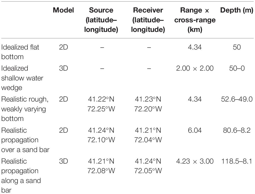
Table 1. Summary of scenarios considered in underwater sound propagation simulations.
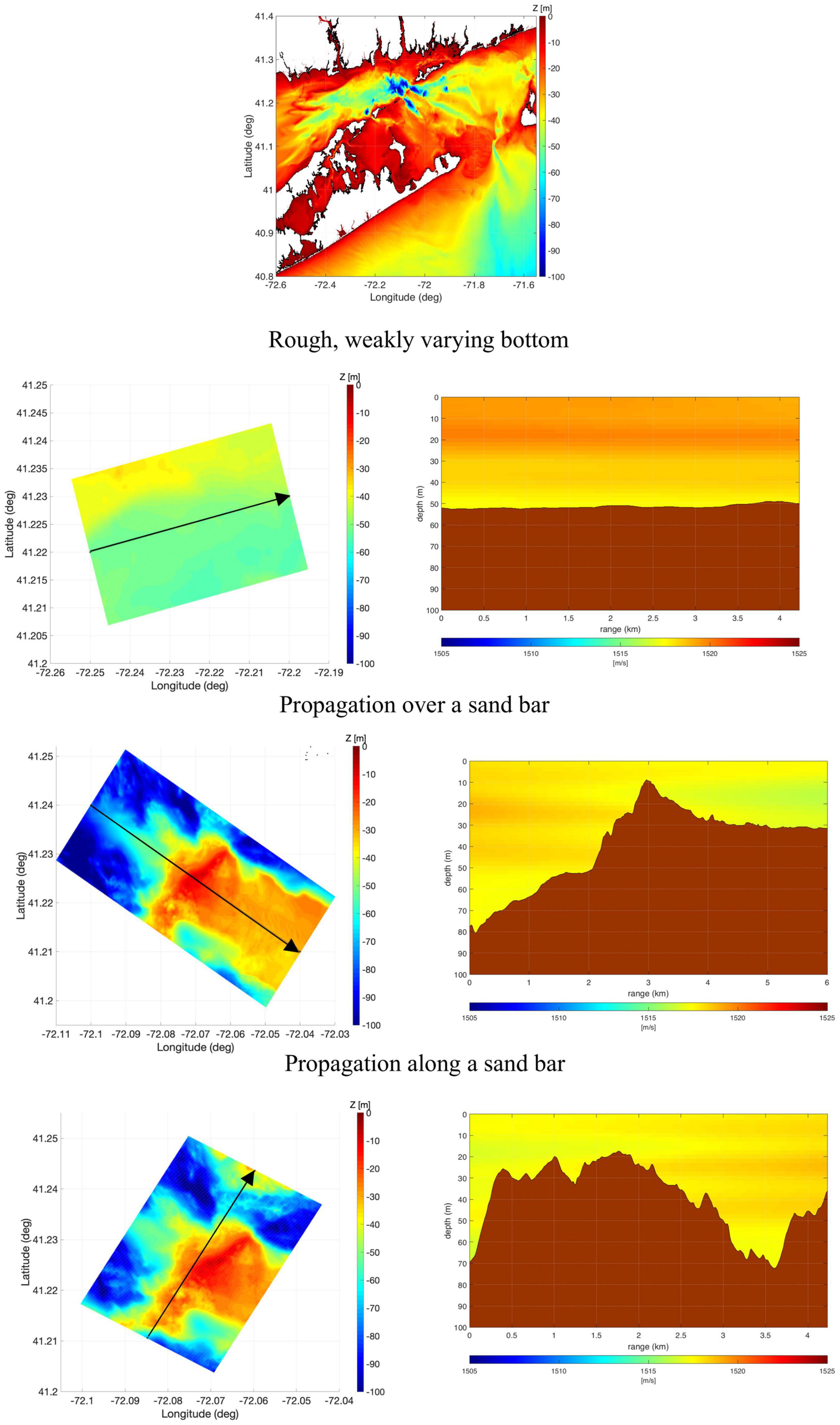
Figure 1. Bathymetry of Long Island Sound (top panel). Bathymetry and sound speed for the propagation scenarios: rough, weakly varying bottom flat bottom (second panel), propagation over a sand bar (third panel), and propagation along a sand bar (bottom panel). Plots on the right present bathymetry and sound speed profiles along the central line of the propagation domains denoted by the arrow over the bathymetry map (plots on the left).
Three types of sound speed profiles (SSPs) are also considered in the simulations: (a) SSP constant c0 = 1500m/s, (b) SSP range-independent c(z), and (c) SSP range-dependent c(r,z), where r is the range and z depth. The latter two SSP scenarios are based on temperature and salinity from the Regional Ocean Modeling System (ROMS) Experimental System for Predicting Shelf and Slope Optics (ESPreSSO) model covering the Mid-Atlantic Bight (Rutgers Ocean Modeling Group, 2020). The ROMS ESPreSSO model has a 5-km horizontal resolution and 36-levels in the water column. Sound speed fields are derived from temperature and salinity based on the Mackenzie (1981) equation. For the sake of simplicity, only results from one ROMS-ESPreSSO time is used. Then, simulations represent environmental condition for September 10, 2018 at 00:00.
Numerical Results
Simulations for a 500 and 1500 Hz source were performed for all the idealized and realistic scenarios with a sound source placed at a 20-m depth. The properties of the bottom considered in all the simulations are sound speed cb = 1700m/s, density ρ = 1500kg/m3 and attenuation βb = 0.5 dB/λ, where λ is the wavelength. Also, for all the simulations, water density is considered to be a constant of ρw = 1000 kg/m3.
Numerical results are presented first for the idealized scenarios and then for the realistic scenarios in the following order: (i) 2D flat bottom, (ii) 3D shallow water wedge, (iii) 2D rough, weakly varying bottom, (iv) 2D propagation over a sand bar, and (v) 3D propagation along a sand bar. In the realistic scenarios, the bathymetry and SSPs considered in the 2D simulations correspond to the central part (y = 0, where y is the cross-range) of the propagation domains (see Figure 1).
Idealized 2D Flat Bottom
The performance of the 2D versions of PE, Kraken, and Bellhop is compared on a 50-m flat bottom with SSP constant (c0 = 1500m/s). This simple comparison aims to calibrate the models and ensure that potential differences on more complex simulations are not due to incorrect model setups.
In PE and normal mode models, different frequencies require different numerical discretizations. As the wavelength reduces with increasing frequency, smaller spatial distances between calculation points must be used. Therefore, higher resolutions should be used in a PE model in the range (Δx) and water depth (Δz). Likewise, Δz should be smaller for higher frequencies in Kraken, leading to more computational points and increasing the computational cost. As a rule of thumb, to solve the normal mode equation accurately in Kraken, a minimum of 10 points per wavelength should be considered in the water column (z). A Δx smaller or equal to one wavelength and Δz approximately lower or equal than one-quarter of wavelength should be used in PE simulations.
For simplicity, the minimum required numerical discretizations were calculated for the most demanding frequency, 1500 Hz (nominal wavelength of 1 m), and also used for 500 Hz (nominal wavelength of 3 m). A grid with Δx = Δz = 0.1 m was used in Kraken and PE 2D simulations, which correspond to a very high resolution in range. It should be noticed that under standard conditions, the PE needs a much higher range resolution than Kraken-Field to run and provide a result. On the other hand, Kraken-Field can run with lower range resolution. However, if sharp bathymetric or sound speed variations are present, Kraken-Field cannot provide accurate results considering a low range resolution.
In the Bellhop simulations, 10000 Gaussian beams launched in an angular fan from −70° and 70° angle were considered. Bellhop settings were decided from a series of numerical convergence tests. Figure 2 compares transmission loss (TL) obtained by the three models for the flat bottom with the isovelocity waveguide. The agreement among the three models for this scenario is excellent for both 1500 and 500 Hz.
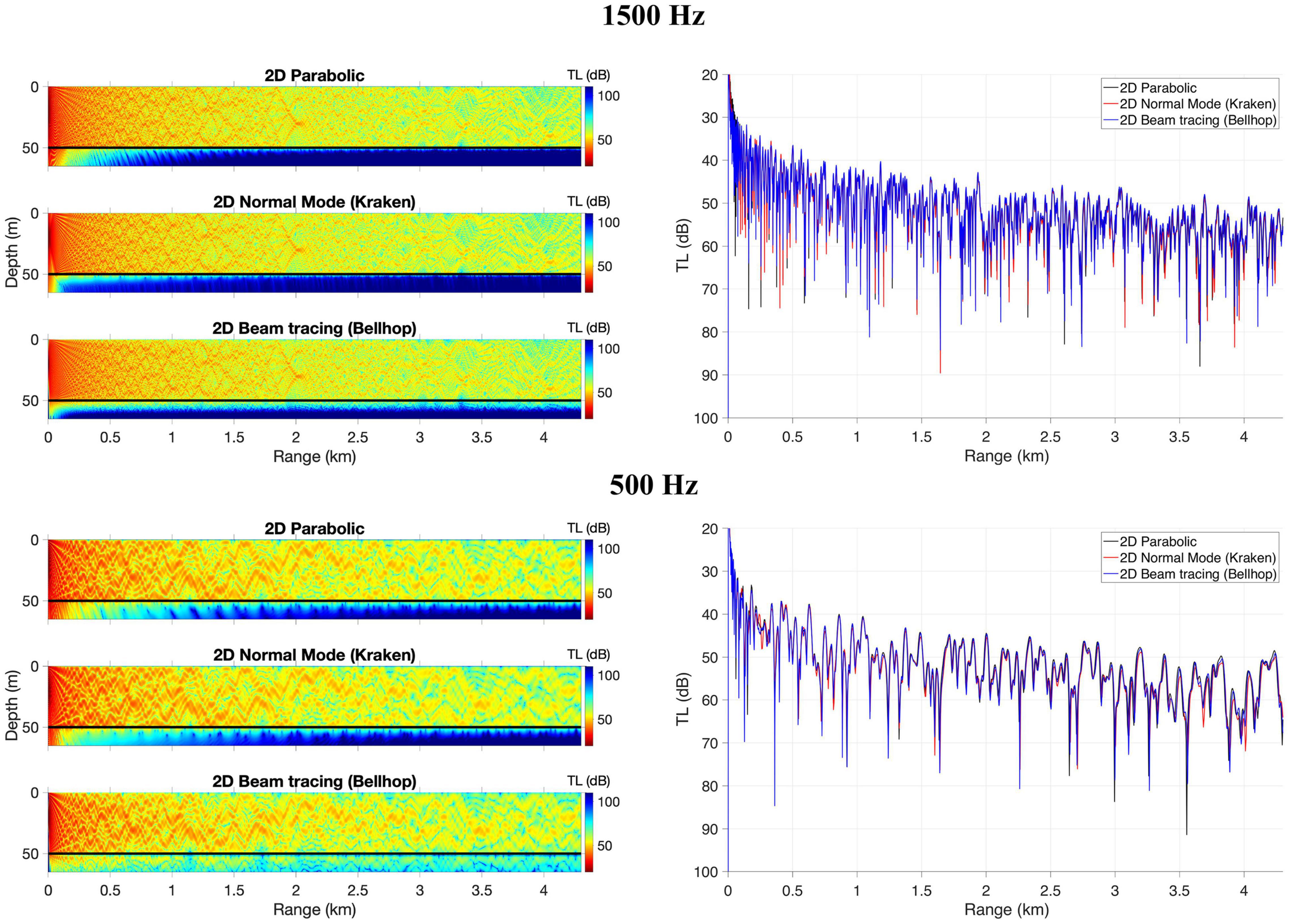
Figure 2. Transmission loss for a 1500 Hz (top panel) and 500 Hz (bottom panel) sound source for an isovelocity (c0 = 1500m/s) waveguide with a flat bottom. Plots on the right present TL over the range at 20 m water depth. Results are presented for 2D parabolic, 2D normal mode (Kraken, mode coupling), and 2D beam tracing (Bellhop).
Idealized 3D Shallow Water Wedge
An idealized shallow water wedge case (see Figure 3) is simulated with the 3D versions of PE, Kraken, and Bellhop for 500 and 1500 Hz. This case is a shallow water higher frequency adaptation of the wedge problem with a penetrable lossy bottom proposed by Jensen and Ferla (1990) for the Acoustical Society of America (ASA) and has been widely used by the underwater acoustic modeling community for 3D model validation and to study 3D horizontal reflection (e.g., Lin, 2019; Porter, 2019). Similar to the Jensen and Ferla’s wedge problem, the slope angle of the shallow water wedge is π/63 rad (1/20 slope), the sound speed in the water is 1500 m/s and the density is 1000 kg/m3; the sound speed in the bottom is cb = 1700m/s, and the density is ρ = 1500 kg/m3. The bottom also incorporates a volume attenuation of βb = 0.5 dB per wavelength. However, in the shallow water wedge, a point source of unit intensity is placed 1 km (horizontal distance) away from the wedge at 20 m depth below the sea surface. The water depth at the source is 50 m, intending to represent the typical characteristics of the propagation domains chosen for Long Island Sound.
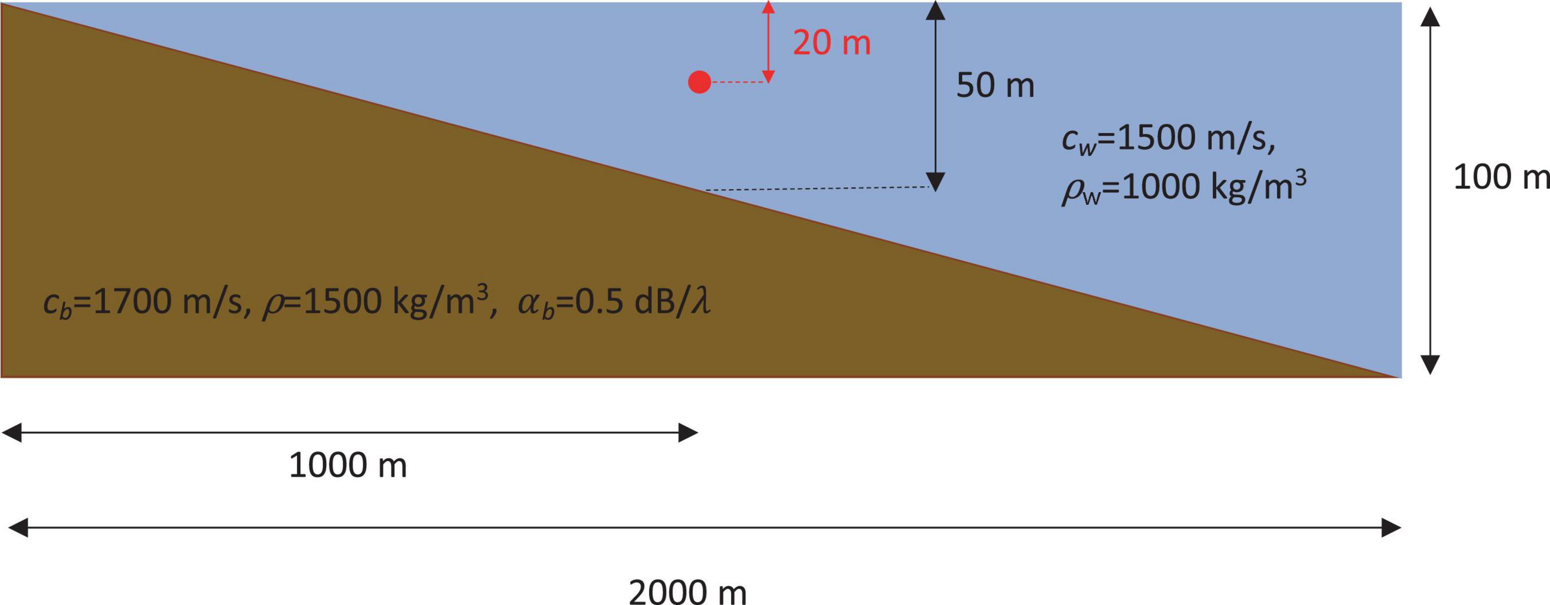
Figure 3. Schematic diagram of the idealized shallow water wedge. Red dot presents the sound source.
In the PE simulations, the marching (range) and transverse (cross-range) grid size for 500 Hz was set to be 0.5 and 0.25 m, respectively. These values decreased to 0.25 and 0.125 m, respectively, for 1500 Hz. In the water depth, the grid size was set to 0.2 and 0.1 m for 500 and 1500 Hz, respectively. Parabolic and Bellhop results for the shallow water wedge scenario agree very well (see Figure 4). The Kraken solution tends to fall after 1.0 km for 1500 Hz and after 0.2 km for 500 Hz. The errors found in 3D Kraken solution are due to neglecting the mode coupling in the model. Sound propagation over a bathymetry like a wedge can induce strong horizontal refraction and mode coupling, which makes it challenging for a model that neglects mode coupling to provide an accurate solution.
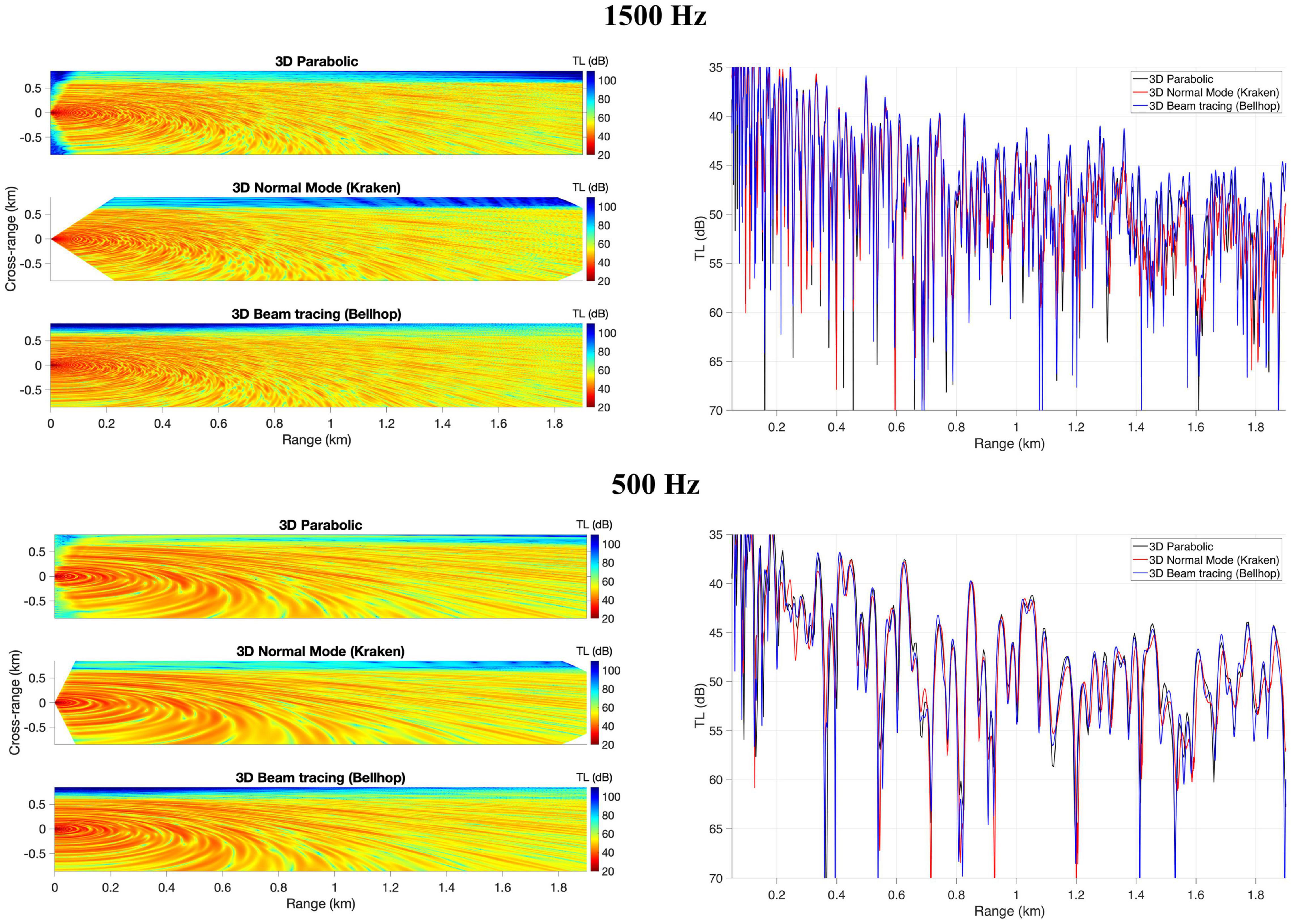
Figure 4. Comparison between 3D parabolic, 3D normal mode (Kraken, no mode coupling), and 3D beam tracing (Bellhop) for the shallow water wedge problem. Results present TL at 20 m depth for a 1500 Hz (top panel) and 500 Hz (bottom panel) sound source for an isovelocity (c0 = 1500m/s) waveguide. Plots on the right present TL at cross-range = 0.
Realistic 2D Rough, Weakly Varying Bottom
The rough, weakly varying bottom scenario results are presented in Figure 5 for the 2D versions of PE, Kraken, and Bellhop. The range-independent SSP c(z) is used. The same model parameters considered in the flat bottom scenario (see section “Idealized 2D Flat Bottom”) are used here. Overall, the three models agree very well near the source. However, after about 3 km in distance, some minor differences between the three model solutions can be observed for both 500 and 1500 Hz. Although the three solutions are still comparable, the agreement is not as well as the 2D flat bottom case shown in section “Idealized 2D Flat Bottom.” In this realistic case, the PE solution tends to be closer to Kraken than the Bellhop solution. Differences can be due to the interpolation of environment (bathymetry and SSP) variables over depth and range. In this regard, PE and Kraken use stair-step profiles to approximate the rough bottom interface condition. The simulation of this scenario highlights the challenge of considering the same waveguide parameters in the three models for the same environmental data.
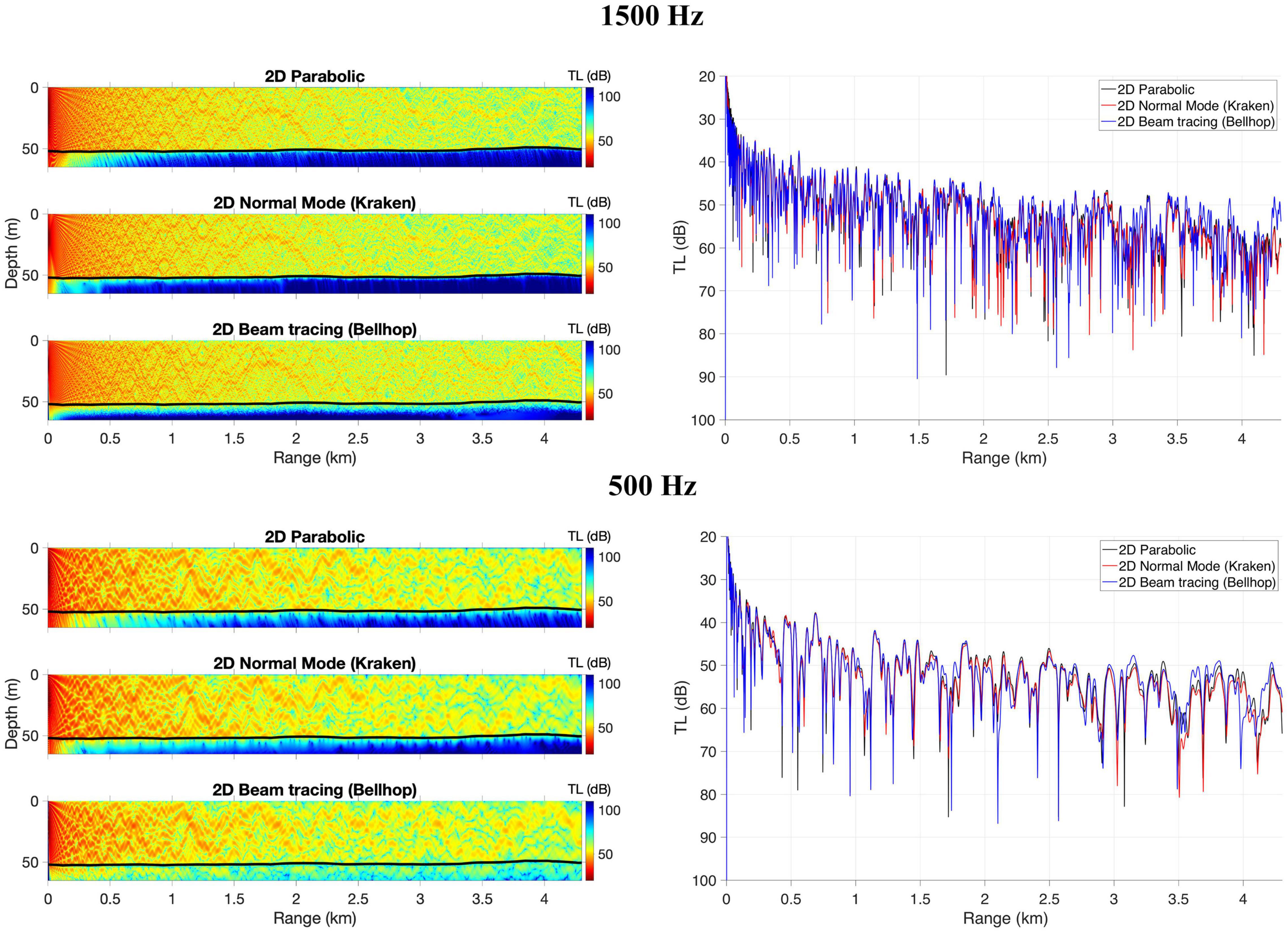
Figure 5. Transmission loss for a 1500 Hz (top panel) and 500 Hz (bottom panel) sound source for an SSP range-independent [c(z)] waveguide with a rough, weakly varying bottom. Plots on the right present TL over the range at 20 m water depth. Results are presented for 2D parabolic, 2D normal mode (Kraken, mode coupling), and 2D beam tracing (Bellhop).
Realistic 2D Propagation Over a Sand Bar
Transmission loss results from the PE, normal mode and beam tracing models for sound propagation over a sand bar are presented with the range-dependent SSP c(r, z) in Figure 6. These results are all done on a 2D slice, neglecting horizontal refraction. This particular case cuts through the bottom because the receiver is at 20 m (plots on the right of Figure 6), and the seafloor shallows to nearly 8 m deep at the sand bar. The bathymetry of this scenario presents a steep slope at the beginning, with bathymetry changing in 3 km from approximately 80 m depth to the top of the sand bar. After the top of the sand bar, the depth increases again to 30 m, and then bathymetry presents slight changes for 2 km. As it is observed in Figure 6, PE and Kraken TL comparison looks very good, with 1–2 dB differences in the peak levels after the sand bar. Bellhop agrees with PE and Kraken before the sound reaches the sand bar. However, the quality of Bellhop results tends to fall after beams cross the top of the sand bar. It should be noted that going down to 1500 Hz is pushing a ray model a bit for these water depths. With the complicated bathymetry of the propagation over a sand bar scenario and diffraction happening at every break in the profile, it can be considered hard for a ray model to track the interference pattern. Also, the low-frequency case of 500 Hz at such shallow water is below the threshold of a ray/beam code’s validity.
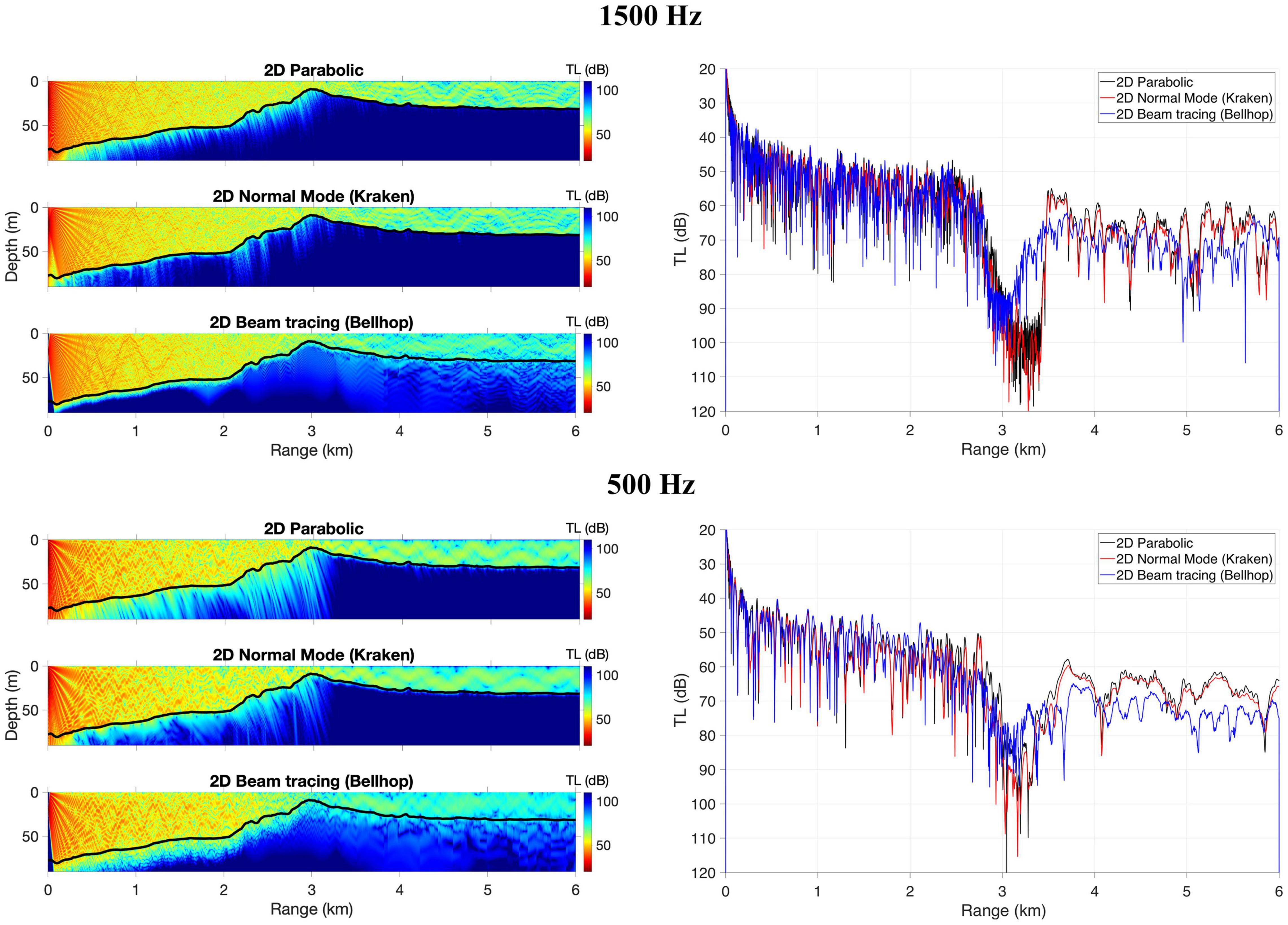
Figure 6. Transmission loss for a 1500 Hz (top panel) and 500 Hz (bottom panel) sound source propagating over a sand bar with an SSP range-dependent [c(r,z)] waveguide. Plots on the right present TL over the range at 20 m water depth. Results are presented for 2D parabolic, 2D normal mode (Kraken, mode coupling), and 2D beam tracing (Bellhop).
Realistic 3D Propagation Along a Sand Bar
With the PE model being tested in simpler environmental scenarios, simulations were carried out for the propagation along a sand bar with the range-dependent SSP c(r, z) to investigate 3D effects. The same model parameters values used in the shallow water wedge scenario are used here. Apart from the 3D simulations, the azimuth independent Nx2D simulations were also performed. This type of simulation used a 2D model with the same PE technique but neglected the transverse coupling of sound energy and only considered its variation in the radial direction. A comparison between 3D and Nx2D results identifies 3D propagation effects that 2D models cannot detect.
Focusing and horizontal refraction can be seen in the 3D model at different ranges. However, these effects are not reproduced by the Nx2D model (see Figure 7). These 3D effects are clearly induced by the bathymetric changes along the propagation paths. For instance, between 1.5 and 2.8 km range, where the sound bar reaches the lowest depths (from 20 to 10 m depth) at cross-ranges between 0.0 and 0.5 km, strong horizontal reflection can be observed on 3D results. Differences between 3D and Nx2D depth-integrated intensity are higher for 500 Hz than 1500 Hz.
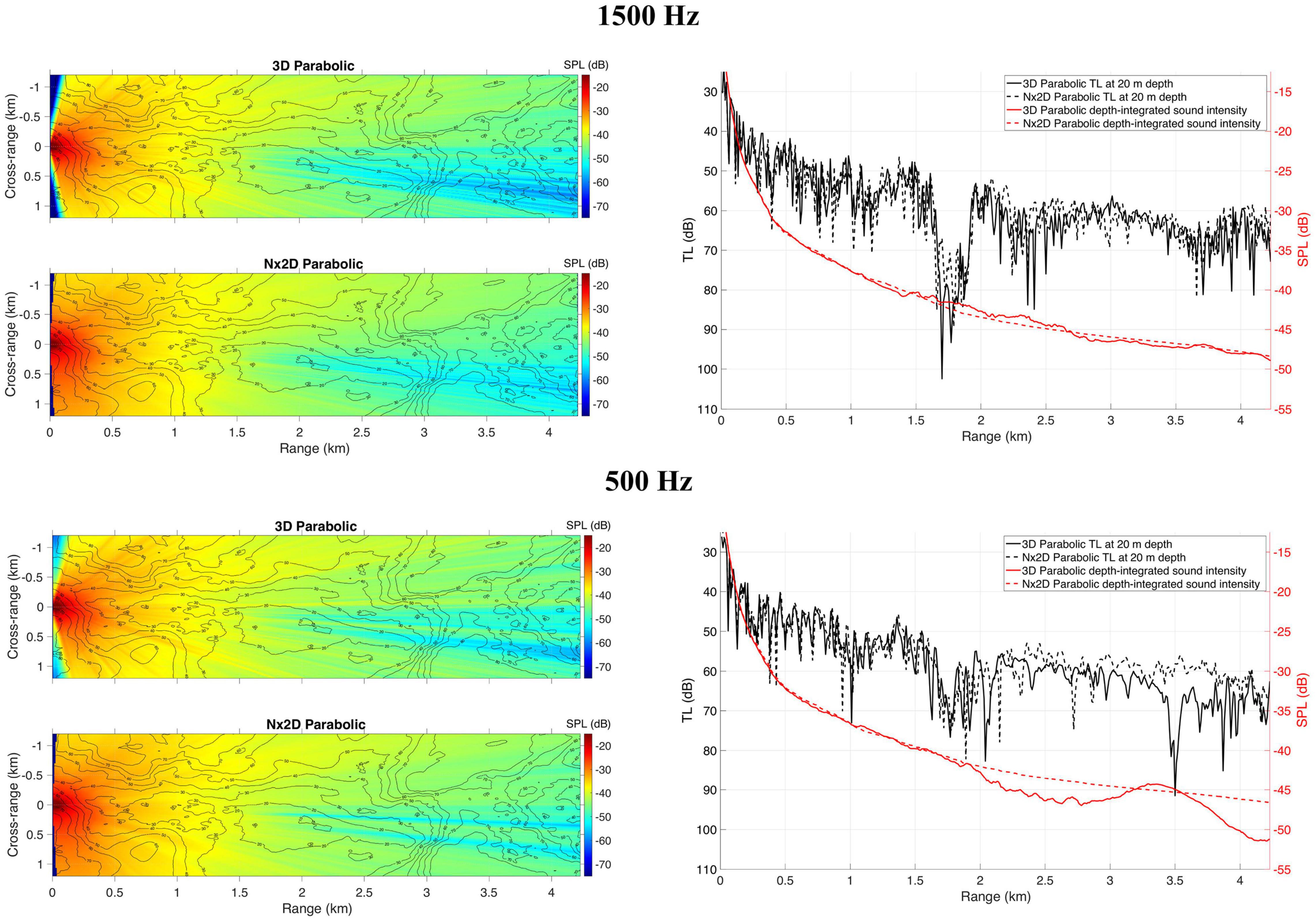
Figure 7. Comparison between 3D parabolic and Nx2D parabolic results for sound propagating along a sand bar and SSP range-dependent [c(r,z)] and for 1500 Hz (top panel) and 500 Hz (bottom panel). Plots on the left are for depth-integrated sound intensity from a 0 dB source. Plots on the right present depth-integrated sound intensity and TL at 20 m depth for cross-range = 0.
Conclusion
A 3D PE underwater sound propagation model was applied to the complex shallow water environment in Long Island Sound, off the United States east coast. First, the 2D and 3D versions of the PE model were compared with state-of-the-art normal mode and beam tracing models for two idealized cases representative of the local environment: (i) a 2D 50-m flat bottom, and (ii) a 3D shallow water wedge. After verifying its performance by comparing to the normal mode and beam tracing models, the PE model is utilized to simulate sound propagation in three realistic local scenarios. Frequencies of 500 and 1500 Hz are considered in all the simulations. Bathymetric models were constructed based on a high-resolution bathymetry (∼10 m horizontal resolution) dataset. Three different realistic sound speed fields were considered in the simulations (constant value, constant profile over the range, and range-dependent).
Overall, TL results provided by the PE, normal mode, and beam tracing models tend to agree with each other. However, differences can emerge with increasing the bathymetry complexity and expanding the range of propagation. For the complex shallow bathymetry found in some areas of Long Island Sound, it can be indeed considered challenging for the models to track the interference sound pattern. Also, the low-frequency cases of 500 Hz at such shallow water are below the threshold of a ray/beam model’s validity. In this regard, the model results indicate that when choosing an underwater sound propagation model for practical applications in a complex shallow water environment, a compromise will be made between numerical model accuracy, computational time, and validity.
Results obtained with 3D PE suggest that in the shallow water environment of Long Island Sound bathymetric features such as sand bars can induce significant 3D effects on sound propagation. These effects were confirmed to happen more often for 500 Hz than 1500 Hz sound and can occur, for instance, on sound propagating along local sand bars. This can potentially affect the underwater soundscape dominated by low frequency marine traffic sound in the area.
The methodology used in this study can also be used for other 3D underwater sound propagation studies. More specifically, before using the 3D model, its 2D version can be compared with other state-of-the-art models. In this way, a better understanding of model performance and limitations can be obtained. Moreover, this inter-model comparison can be used as model calibration when field acoustic data is not available for validating the model.
Although this investigation is focused on Long Island Sound, it can provide helpful information for underwater acoustic applications in other shallow areas. This fact assumes special significance given the increasing interest in using underwater acoustic modeling for environmental impacts assessments. Future work also includes inter-model comparison in shallow water environments considering more physical processes known to influence sound propagation, such as scattering from the sea surface. Passive acoustic monitoring of the underwater soundscape with distributed hydrophone arrays in Long Island Sound is also suggested to investigate the 3D propagation effects shown in the modeling work reported in this article.
Data Availability Statement
Kraken and Bellhop input files are available upon request.
Author Contributions
TO: numerical simulations, methodology, formal analysis, and writing – original draft. Y-TL and MP: methodology, formal analysis, and writing – review and editing. All authors contributed to the article and approved the submitted version.
Funding
TO thanks FCT/MCTES for the financial support to CESAM (UIDP/50017/2020 + UIDB/50017/2020), through national funds. The funding support from the Office of Naval Research for Y-TL via the grant N00014-21-1-2416 was also acknowledged. MP was supported by the Office of Naval Research under contracts N68335-17-C-0553 and N00014-18-C-7007.
Conflict of Interest
MP was employed by company Heat, Light, and Sound Research, Inc.
The remaining authors declare that the research was conducted in the absence of any commercial or financial relationships that could be construed as a potential conflict of interest.
Publisher’s Note
All claims expressed in this article are solely those of the authors and do not necessarily represent those of their affiliated organizations, or those of the publisher, the editors and the reviewers. Any product that may be evaluated in this article, or claim that may be made by its manufacturer, is not guaranteed or endorsed by the publisher.
References
Avilov, K. V. (1995). Pseudodifferential parabolic equations of sound propagation in the slowly range-dependent ocean and their numerical solutions. Acoust. Phys. 41, 1–7. doi: 10.1007/978-1-4613-2201-6_1
Ballard, M. S., Goldsberry, B. M., and Isakson, M. J. (2015). Normal mode analysis of three-dimensional propagation over a small-slope cosine shaped hill. J. Comput. Acoust. 23:1550005. doi: 10.1142/s0218396x15500058
Bucker, H. P. (1994). A simple 3D gaussian beam sound propagation model for shallow water. J. Acoust. Soc. Am. 95, 2437–2440. doi: 10.1121/1.409853
Calazan, R., and Rodríguez, O. (2018). Simplex based three-dimensional eigenray search for underwater predictions. J. Acoust. Soc. Am. 143, 2059–2065.
Červený, V., Popov, M. M., and Pšenčík, I. (1982). Computation of wave fields in inhomogeneous media—Gaussian beam approach. Geophys. J. Int. 70, 109–128. doi: 10.1111/j.1365-246x.1982.tb06394.x
Collins, M. D. (1993). A split-step Padé solution for the parabolic equation method. J. Acoust. Soc. Am. 93, 1736–1742. doi: 10.1121/1.406739
Dahl, P. H., and Dall’Osto, D. R. (2017). On the underwater sound field from impact pile driving: arrival structure, precursor arrivals, and energy streamlines. J. Acoust. Soc. Am. 142, 1141–1155. doi: 10.1121/1.4999060
DeCourcy, B. J., and Duda, T. F. (2020). A coupled mode model for omnidirectional three-dimensional underwater sound propagation. J. Acoust. Soc. Am. 148, 51–62. doi: 10.1121/10.0001517
Dekeling, R. P. A., Tasker, M. L., Van der Graaf, A. J., Ainslie, M. A., Andersson, M. H., André, M., et al. (2014). Monitoring Guidance for Underwater Noise in European Seas, Part I: Executive Summary. A guidance document within the Common Implementation Strategy for the Marine Strategy Framework Directive by MSFD Technical Subgroup on Underwater Noise. Luxembourg: Publications Office of the European Union.
Duarte, C. M., Chapuis, L., Collin, S. P., Costa, D. P., Devassy, R. P., Eguiluz, V. M., et al. (2021). The soundscape of the Anthropocene ocean. Science 371:eaba4658.
Duda, T. F., Lin, Y.-T., and Reeder, D. B. (2011). Observationally constrained modeling of sound in curved ocean internal waves: examination of deep ducting and surface ducting at short range. J. Acoust. Soc. Am. 130, 1173–1187. doi: 10.1121/1.3605565
Hastie, G. D., Russell, D. J., McConnell, B., Moss, S., Thompson, D., and Janik, V. M. (2015). Sound exposure in harbour seals during the installation of an offshore wind farm: predictions of auditory damage. J. Appl. Ecol. 52, 631–640. doi: 10.1111/1365-2664.12403
Heaney, K. D., and Campbell, R. L. (2016). Three-dimensional parabolic equation modeling of mesoscale eddy deflection. J. Acoust. Soc. Am. 139, 918–926. doi: 10.1121/1.4942112
Jensen, F. B., and Ferla, C. M. (1990). Numerical solutions of range-dependent benchmark problems in ocean acoustics. J. Acoust. Soc. Am. 87, 1499–1510. doi: 10.1121/1.399448
Jensen, F. B., Kuperman, W. A., Porter, M. B., and Schmidt, H. (2011). Computational Ocean Acoustics. Berlin: Springer Science and Business Media.
Jenserud, T., and Ivansson, S. (2015). Measurements and modeling of effects of out-of-plane reverberation on the power delay profile for underwater acoustic channels. IEEE J. Ocean. Eng. 40, 807–821. doi: 10.1109/joe.2015.2475675
Jones, R. M., Riley, J. P., and Georges, T. M. (1986). HARPO: A Versatile Three-Dimensional Hamiltonian Ray-Tracing Program for Acoustic Waves in an Ocean with Irregular Bottom. National Oceanic and Atmospheric Administration Environmental Research Laboratories Report. Boulder, CO: Wave Propagation Laboratory.
Lee, D., Botseas, G., and Siegmann, W. L. (1992). Examination of three-dimensional effects using a propagation model with azimuth-coupling capability (FOR3D). J. Acoust. Soc. Am. 91, 3192–3202. doi: 10.1121/1.402856
Lin, Y.-T. (2019). Three-dimensional boundary fitted parabolic-equation model of underwater sound propagation. J. Acoust. Soc. Am. 146, 2058–2067. doi: 10.1121/1.5126011
Lin, Y.-T., and Duda, T. F. (2012). A higher-order split-step Fourier parabolic-equation sound propagation solution scheme. J. Acoust. Soc. Am. 132, EL61–EL67.
Lin, Y.-T., Newhall, A. E., Miller, J. H., Potty, G. R., and Vigness-Raposa, K. J. (2019). A three-dimensional underwater sound propagation model for offshore wind farm noise prediction. J. Acoust. Soc. Am. 145, EL335–EL340.
Luo, W., and Schmidt, H. (2009). Three-dimensional propagation and scattering around a conical seamount. J. Acoust. Soc. Am. 125, 52–65. doi: 10.1121/1.3025903
Mackenzie, K. V. (1981). Nine-term equation for sound speed in the oceans. J. Acoust. Soc. Am. 70, 807–812. doi: 10.1121/1.386920
National Geophysical Data Center [NGDC] (2007). Montauk, New York 1/3 Arc-Second MHW Coastal Digital Elevation Model. Asheville, CL: National Centers for Environmental Information.
Oliveira, T. C. A., and Lin, Y.-T. (2019). Three-dimensional global scale underwater sound modeling: the T-phase wave propagation of a Southern Mid-Atlantic Ridge earthquake. J. Acoust. Soc. Am. 146, 2124–2135. doi: 10.1121/1.5126010
Pekeris, C. L. (1948). Theory of propagation of explosive sound in shallow water. Geol. Soc. Am. Mem. 27.
Petrov, P. S., Ehrhardt, M., Tyshchenko, A. G., and Petrov, P. N. (2020). Wide-angle mode parabolic equations for the modelling of horizontal refraction in underwater acoustics and their numerical solution on unbounded domains. J. Sound Vib. 484:115526. doi: 10.1016/j.jsv.2020.115526
Porter, M. B. (2019). Beam tracing for two-and three-dimensional problems in ocean acoustics. J. Acoust. Soc. Am. 146, 2016–2029. doi: 10.1121/1.5125262
Porter, M.B. (1992). The KRAKEN Normal Mode Program (No. NRL/MR/5120-92-6920). Washington, DC: Naval Research Lab.
Reeder, D. B., and Lin, Y.-T. (2019). 3D acoustic propagation through an estuarine salt wedge at low-to-mid-frequencies: modeling and measurement. J. Acoust. Soc. Am. 146, 1888–1902. doi: 10.1121/1.5125258
Reilly, S. M., Potty, G. R., and Thibaudeau, D. (2016). Investigation of horizontal refraction on Florida Straits continental shelf using a three-dimensional Gaussian ray bundling model. J. Acoust. Soc. Am. 140, EL269–EL273.
Rutgers Ocean Modeling Group (2020). ESPRESSO Ocean Modeling From Rutgers ROMS Group. Available online at: http://www.myroms.org/espresso/ (accessed March 7, 2020).
Shannon, G., McKenna, M. F., Angeloni, L. M., Crooks, K. R., Fristrup, K. M., Brown, E., et al. (2016). A synthesis of two decades of research documenting the effects of noise on wildlife. Biol. Rev. 91, 982–1005. doi: 10.1111/brv.12207
Smith, K. B. (1999). A three-dimensional propagation algorithm using finite azimuthal aperture. J. Acoust. Soc. Am. 106, 3231-3239.
Sturm, F. (2005). Numerical study of broadband sound pulse propagation in three-dimensional oceanic waveguides. J. Acoust. Soc. Am. 117, 1058-1079.
Tappert, F. D. (1977). “The parabolic equation method,” in Wave Propagation and Underwater Acoustics, eds J. B. Keller and J. Papadakis, Vol. 70 (New York, NY: Springer), 224–286.
Thomson, D. J., and Chapman, N. R. (1983). A wide-angle split-step algorithm for the parabolic equation. J. Acoust. Soc. Am. 74, 1848-1854.
Keywords: underwater soundscape, 3D PE, Bellhop3D, Kraken3D, Long Island Sound, sand bars
Citation: Oliveira TCA, Lin Y-T and Porter MB (2021) Underwater Sound Propagation Modeling in a Complex Shallow Water Environment. Front. Mar. Sci. 8:751327. doi: 10.3389/fmars.2021.751327
Received: 31 July 2021; Accepted: 17 September 2021;
Published: 15 October 2021.
Edited by:
Ana Širovic, Norwegian University of Science and Technology, NorwayReviewed by:
Peter Dahl, University of Washington, United StatesPavel Petrov, V.I. Il’Ichev Pacific Oceanological Institute, Russian Academy of Sciences (RAS), Russia
Copyright © 2021 Oliveira, Lin and Porter. This is an open-access article distributed under the terms of the Creative Commons Attribution License (CC BY). The use, distribution or reproduction in other forums is permitted, provided the original author(s) and the copyright owner(s) are credited and that the original publication in this journal is cited, in accordance with accepted academic practice. No use, distribution or reproduction is permitted which does not comply with these terms.
*Correspondence: Tiago C. A. Oliveira, dG9saXZlaXJhQHVhLnB0