Evaluating the Efficacy of Acoustic Metrics for Understanding Baleen Whale Presence in the Western North Atlantic Ocean

Pegg, Nicole; Roca, Irene T.; Cholewiak, Danielle; Davis, Genevieve E.; Van Parijs, Sofie M.

doi:10.3389/fmars.2021.749802

ORIGINAL RESEARCH article

Front. Mar. Sci., 22 October 2021

Sec. Ocean Observation

Volume 8 - 2021 | https://doi.org/10.3389/fmars.2021.749802

This article is part of the Research Topic Innovation and Discoveries in Marine Soundscape Research View all 20 articles

Evaluating the Efficacy of Acoustic Metrics for Understanding Baleen Whale Presence in the Western North Atlantic Ocean

$\r\nNicole Pegg,$ Nicole Pegg^1,2

Irene T. Roca^3,4

Danielle Cholewiak¹

Genevieve E. Davis¹

Sofie M. Van Parijs^1*

¹Northeast Fisheries Science Center, National Marine Fisheries Service, National Oceanic and Atmospheric Administration, Woods Hole, MA, United States
²Harbor Branch Oceanographic Institute, Florida Atlantic University, Fort Pierce, FL, United States
³Helmholtz Institute for Functional Marine Biodiversity, University of Oldenburg, Oldenburg, Germany
⁴Ocean Acoustics Lab, Alfred Wegener Institute, Helmholtz Centre for Polar and Marine Research, Bremerhaven, Germany

Soundscape analyses provide an integrative approach to studying the presence and complexity of sounds within long-term acoustic data sets. Acoustic metrics (AMs) have been used extensively to describe terrestrial habitats but have had mixed success in the marine environment. Novel approaches are needed to be able to deal with the added noise and complexity of these underwater systems. Here we further develop a promising approach that applies AM with supervised machine learning to understanding the presence and species richness (SR) of baleen whales at two sites, on the shelf and the slope edge, in the western North Atlantic Ocean. SR at both sites was low with only rare instances of more than two species (out of six species acoustically detected at the shelf and five at the slope) vocally detected at any given time. Random forest classification models were trained on 1-min clips across both data sets. Model outputs had high accuracy (>0.85) for detecting all species’ absence in both sites and determining species presence for fin and humpback whales on the shelf site (>0.80) and fin and right whales on the slope site (>0.85). The metrics that contributed the most to species classification were those that summarized acoustic activity (intensity) and complexity in different frequency bands. Lastly, the trained model was run on a full 12 months of acoustic data from on the shelf site and compared with our standard acoustic detection software and manual verification outputs. Although the model performed poorly at the 1-min clip resolution for some species, it performed well compared to our standard detection software approaches when presence was evaluated at the daily level, suggesting that it does well at a coarser level (daily and monthly). The model provided a promising complement to current methodologies by demonstrating a good prediction of species absence in multiple habitats, species presence for certain species/habitat combinations, and provides higher resolution presence information for most species/habitat combinations compared to that of our standard detection software.

Introduction

Soundscapes comprise the complex variety of biological, anthropogenic, and environmental sounds of a given habitat (Krause, 2008; Pijanowski et al., 2011). They provide a unique perspective into a given ecosystem, whether terrestrial or marine, due to the integrative approach of studying all sounds of an environment together (e.g., Farina, 2013). However, recent capacity increases in long-term acoustic data collection are challenging scientists to develop new and creative ways to analyze these complex data (e.g., Gibb et al., 2019). Extracting variability in patterns and measuring diversity in these data frequently requires taking a number of approaches. McKenna et al. (submitted to this research topic) define soundscape analyses as viewing a question through different lenses by dividing them into biodiversity assessments, human impacts, and the acoustic scene analysis, with each view requiring different approaches and metrics. Which analyses or metrics are most appropriate depends on the “lens” with which one is interested in interpreting the data. Various approaches for analyzing soundscape data range from long-term ambient sound measurements, observing variation in sound pressure levels, and using individual or a combination of acoustic metrics (AMs) (e.g., Sueur et al., 2014; Kaplan et al., 2015; Haver et al., 2018; Bradfer-Lawrence et al., 2019).

Acoustic metrics refer to a number of standardized and automated metrics that can comprise acoustic diversity indices such as Acoustic Complexity Index, entropy, evenness, and roughness (e.g., Sueur et al., 2014; Bradfer-Lawrence et al., 2019; Farina et al., 2021), as well as specific metrics on the spectral and temporal patterns of the soundscapes such as the spectral integral, the envelope median, and background noise proportion (Boelman et al., 2007; Depraetere et al., 2012; Towsey, 2017). AM can be used singly or in tandem to aggregate complex information from acoustic recordings into a single value. Terrestrial soundscape analyses have applied the use of some AM successfully as proxies for estimating biodiversity (e.g., Sueur et al., 2008), community composition (e.g., Farina et al., 2011), habitat type and vegetation (e.g., Do Nascimento et al., 2020), and ecological condition (e.g., Tucker et al., 2014). Given the success of AM for understanding terrestrial soundscapes, these same AM were applied to the marine environment (e.g., Pieretti et al., 2017; Bohnenstiehl et al., 2018). However, direct application of these approaches to the marine environment have generally not been as successful due to the frequent overlap in frequency bands of biological sounds and background noise that are present, often leading to a lack of a clear relationship between biodiversity and acoustic indices (Mooney et al., 2020). One popular metric, the Acoustic Complexity Index, showed mixed results in describing patterns in the sound assemblages on coral reefs (Mooney et al., 2020). Acoustic indices also were not able to predict bioacoustic activity due to overlap with snapping shrimp and other anthropogenic sounds (Buxton et al., 2018). However, these studies focused on highly complex reef environments. When focusing only on low-frequency data (<125 Hz), Parks et al. (2014) successfully used a single acoustic entropy index to characterize baleen whale calls. Based on these mixed applications of AM there is a need for further developing approaches that can cope better with the heightened prevalence of overlapping sound sources in the marine environment. Solutions could include developing new indices specifically for the marine environment (Parks et al., 2014), using other methods to support assessments like clustering (Mooney et al., 2020), or combining AM in novel ways. Recently, an approach using a number of AM in combination with supervised learning algorithms was successfully used to classify species richness (SR) levels and species identities of marine mammal acoustic communities in the Southern Ocean (Roca and Van Opzeeland, 2019). Here, we evaluate whether this AM analysis approach might be helpful to understanding other marine mammal communities.

Seven baleen whale species are found in the western North Atlantic Ocean, where their distributions often overlap in space and time. These include the North Atlantic right whale (NARW; Eubalaena glacialis), Brydes’ (Balaenoptera edeni), blue (Balaenoptera musculus), fin (Balaenoptera physalus), minke (Balaenoptera acutorostrata), sei (Balaenoptera borealis), and humpback whales (Megaptera novaeangliae). Recently, a decade-long dataset was analyzed using a low-frequency detection and classification system (LFDCS) with species-specific call libraries (Baumgartner and Mussoline, 2011), highlighting North Atlantic right whale year-round use of western North Atlantic Ocean habitat (Davis et al., 2017). In addition, blue, fin, humpback, and sei whales also exhibited wide habitat use in this area, especially in winter when all species were detected throughout the entire data collection range, from the Caribbean to the Greenland Sea (Davis et al., 2020). Minke whale acoustic daily presence was previously described using a different automated acoustic detector, showing seasonal variability and migratory movement throughout the western North Atlantic Ocean (Risch et al., 2014). Bryde’s whales have been acoustically detected in the southern Caribbean (Oleson et al., 2003), but were not included in this study as their range does not typically include the region of the western North Atlantic where most of our acoustic monitoring efforts occur.

While the use and development of species-specific automated detectors are important for bioacoustic analyses, manually reviewing detector output can still be time consuming. Areas of species overlap within baleen whale feeding and migratory routes provide potential sites for methods, like AM, to be useful to gain more knowledge of the acoustic environments and marine mammal community composition in a faster and more streamlined manner. AM can also be applied across different datasets (Roca and Van Opzeeland, 2019), which is necessary when using a wide range of data aimed at understanding baleen whale presence across the western North Atlantic Ocean.

Baleen whales vary in their utilization of shelf, slope, and pelagic habitats throughout their range. In the western North Atlantic Ocean, some species, such as blue whales, have a predominantly pelagic distribution, but can be found seasonally in regions on the continental shelf (e.g., Lesage et al., 2017; Davis et al., 2020). Fin whales occur year-round in on-shelf areas, like Massachusetts Bay (Morano et al., 2012), but also in offshore waters near the Mid-Atlantic ridge (Nieukirk et al., 2012). In contrast, NARWs are generally found in coastal, on-shelf waters (Davis et al., 2017), and can be distributed very close to shore. Due to this species variation in habitat usage, it is important to see how AM perform across different environments.

Previously, success was found in using a suite of AM to characterize the marine mammal community composition in the Southern Ocean with a combination of Balaenopterid, Physeterid, Delphinid, and Phocid species comprising the acoustic assemblages (Roca and Van Opzeeland, 2019). Here, we evaluate if a similar combination of AM and supervised machine learning could help determine the acoustic presence of individual species and SR levels specifically of baleen whales in the western North Atlantic Ocean at the continental shelf and slope sites.

Materials and Methods

Study Sites and Acoustic Recordings

Data were collected from two recording sites in the western North Atlantic Ocean: one located on the continental shelf (hereafter referred to as “shelf”), and the other along the continental slope (“slope”). At the slope site, a High Frequency Acoustic Recording Package (HARP; Wiggins and Hildebrand, 2007) was deployed at a depth of 845 m at 41.06 N, 66.35 W, on the outer United States continental slope near Heezen Canyon, with the hydrophone approximately 20 m above the seafloor (Figure 1 and Table 1). The HARP was programmed to record continuously at a bandwidth rate of 200 kHz from June 11, 2018--May 10, 2019. The HARP was comprised of two transducers; one high-frequency stage using an ITC-1042 hydrophone (International Transducer Corporation), and one low-frequency stage using Benthos AQ-1 transducers¹ (see Table 1 for more technical information). For the purpose of this study, only the low frequency data (<2,000 Hz) were analyzed to best visualize the calls of baleen whale species found in the study area. At the shelf site, a Marine Autonomous Recording Unit (MARU; Clark et al., 2010) was deployed at a depth of 78.6 m at 40.393 N, 70.217 W near the Nantucket Shoals area on the United States continental shelf (Figure 1 and Table 1). The MARU was programmed to record continuously at a 2 kHz sampling rate from December 21, 2016–February 14, 2018 with a gap in data due to battery life constraints from July 15 to 17, 2017 (see Table 1 for additional technical information). Recording sites were selected based on previous analyses of baleen whale acoustic presence in slope and shelf environments around George’s Bank and New England waters (e.g., Risch et al., 2014; Davis et al., 2017, 2020; Weiss et al., 2021).

FIGURE 1

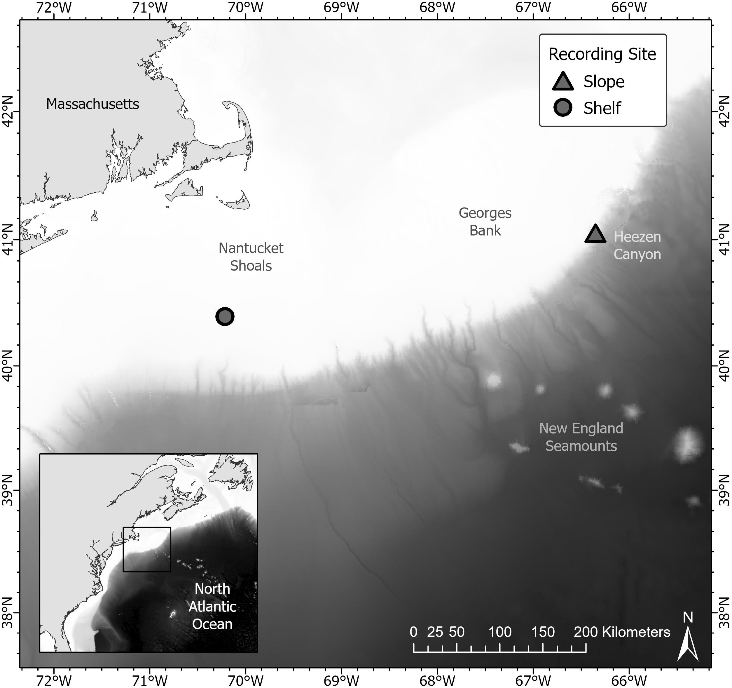
Figure 1. This map shows the location of the two acoustic recording units in the western North Atlantic Ocean used in this study. At the slope site, a High Frequency Acoustic Recording Package (HARP) was located along the continental slope edge near Heezen canyon off of Georges Bank (triangle). At the shelf site, a Marine Autonomous Recording Unit was located near Nantucket Shoals (circle).

TABLE 1

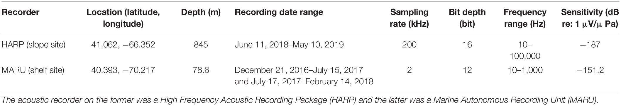
Table 1. This table provides details of the two passive acoustic recorders used for this study, one of which was located along the continental slope and another was located on the shelf.

Acoustic Data Processing and Acoustic Metrics

We performed a stratified random sampling over the complete dataset from the slope and shelf sites to select the acoustic files to constitute our training set (n = 695 and n = 389, respectively). We searched for high quality recordings [i.e., high signal-to-noise ratio (SNR) for species spectral patterns] through as many months and days as possible in order to capture as much temporal, spatial, and species variation in the training set. All sound files for both locations were clipped to 1 min in length for the best call resolution based on baleen whale vocalizations in the study areas. Clipping was performed using Matlab R2017a (The Mathworks, Inc.). We manually assessed species presence/absence in the training set through visual and aural inspection of spectrograms using Raven Pro 2.0 (Cornell Lab of Ornithology, Ithaca, NY, United States). Spectrogram settings were chosen and changed to best help identify different species’ call presence/absence (512pt. FFT for NARW, sei, minke, and humpback; 4096 FFT for fin and blue, Hamming window, 50% overlap).

We defined SR as the number of species acoustically present in a 1-min file, ranging from 0 to 6, and quantified SR for each file based on visual and aural review of the spectrograms. A species was marked absent based on a lack of acoustic presence. We computed 21 different AM (for details on the computed AM see Supplementary Table 1) for every acoustic file in each training set over the full bandwidth 0–1,000 Hz. The AMs that were chosen and the AM parameterization were adapted according to the target species’ call patterns to optimize results. The AM selected were based on their mathematical principles, which had the potential to be the most relevant, and which had already shown to perform well in other marine, specifically marine mammal, acoustic contexts. To account for the complexity and variability in the spectral patterns of the species’ calls, the AEI, ADI, ACI, BI, and NP metrics (see Supplementary Table 1) were computed over four other relevant bandwidths: 10–40; 40–100; 100–200; and 200–900 Hz, for a total of 44 AMs computed per acoustic file. All AMs were computed using R. We used functions from the R package seewave (Sueur et al., 2008) to calculate H, th, sh, ACI, NP, and M, and the R package soundecology (Villanueva-Rivera et al., 2018) to calculate AEI, ADI, BI, and NDSI.

Random Forest Classification Models

We used random forest classification models (Breiman, 2001) to discriminate between the acoustic presence/absence of the different species comprising the acoustic community at each site and to evaluate the discrimination potential of the AMs. Random forest models are widely used tools that show high predictive accuracy and can cope with high-dimensional problems, complex interactions, and even highly correlated predictor variables.

We used the Boruta algorithm (Kursa and Rudnicki, 2010) to select relevant AMs to include as predictor variables in the random forest classification models. The Boruta algorithm iteratively removes the variables that are statistically less relevant than their randomly permuted copies (the random copies’ importance can be non-zero only due to random fluctuations). We used the Boruta function from the Boruta package (Kursa and Rudnicki, 2010) in R.

We used the randomForest function in the R randomForest package (Liaw and Wiener, 2002) to develop the random forest classification models. We ran a hyperparameter grid search for each species model using the R package ranger (Wright and Ziegler, 2015) on values for the total number of trees necessary to stabilize prediction error rates, the number of predictor variables to randomly sample from at each node, the minimum number of samples within the terminal nodes and the maximum number of nodes (both define the degree of model complexity) and finally, the sizes of training and test data subsets to find the best model parameterization according to the above mentioned criteria. We grew 2,001 trees with a node size of 1 and tested between 6 and 16 predictor variables at each split according to the species model. For each tree constructed in the random forest, ∼ 2/3 (0.66–0.75% of data according to species) of the training set were sub-sampled with replacement to train the classification model and ∼ 1/3 was left out as a test subset (i.e., out-of-bag or OOB cases). The general misclassification rate of the model (general OOB estimate) is computed as the average across all OOB cases and trees. We used a conditional permutation scheme (Strobl et al., 2008) to assess variable importance, in order to account for correlations that occurred between some of the AMs. We used the permimp function from the permimp package in R (Debeer and Strobl, 2020) with a 0.80 threshold value. We used the area under the curve (AUC) to compute the permutation importance (Janitza et al., 2013).

Model Predictions and Second-Step Evaluation

To evaluate the performance of the models across a long time series (12 months from January 1 to December 31, 2017), we made a case-study of the models developed for the species recorded at the shelf site. This site was chosen instead of the slope site due to six species being acoustically present instead of six, more diverse combinations of species vocalizing at higher SR levels, and a higher SNR for some species, especially humpback whales, in the clips. We used the generic predict function in R to generate predictions of species presence probabilities on the complete dataset using the trained random forest classification models. We randomly selected 400 1-min acoustic files from the complete dataset and annotated species’ presence/absence using Raven Pro 2.0 as mentioned in section “Acoustic Data Processing and Acoustic Metric” as an independent test set to use as second-step cross validation and evaluation of the species classification models’ performance. To assess the optimal threshold to generate presence/absence scores from the model predicted probabilities in order to evaluate model performance for each species, we used the optimal.thresholds function from the PresenceAbsence package in R (Freeman and Moisen, 2008). We used the confusionMatrix function from the caret package in R (Kuhn, 2020) to conduct the second-step evaluation of models’ performance. We computed a relative daily proportion of acoustic presence for every species as the sum of the 1-min species presence scores per day (obtained by applying the optimal threshold to the estimated probabilities) divided by the total number of minutes recorded per day (i.e., 1,440).

We then compared the modeled outputs summarized as relative daily proportion of acoustic presence with the manually assessed daily acoustic presence of the different baleen whale species for the shelf data set, derived using two acoustic detection software methodologies: LFDCS (Baumgartner and Mussoline, 2011) for NARW (upcall), sei (doublet or triplet down sweeps), blue (A,B, and AB phrases), fin (20 Hz pulse), and humpback (song across multiple years and social sounds) whales (according to Davis et al., 2017, 2020), and an automated pulse train detector (according to Risch et al., 2014) for minke whales (Figure 2). The call types listed above for each individual species were the only call types used when selecting and annotating the 1-min clips for analysis.

FIGURE 2

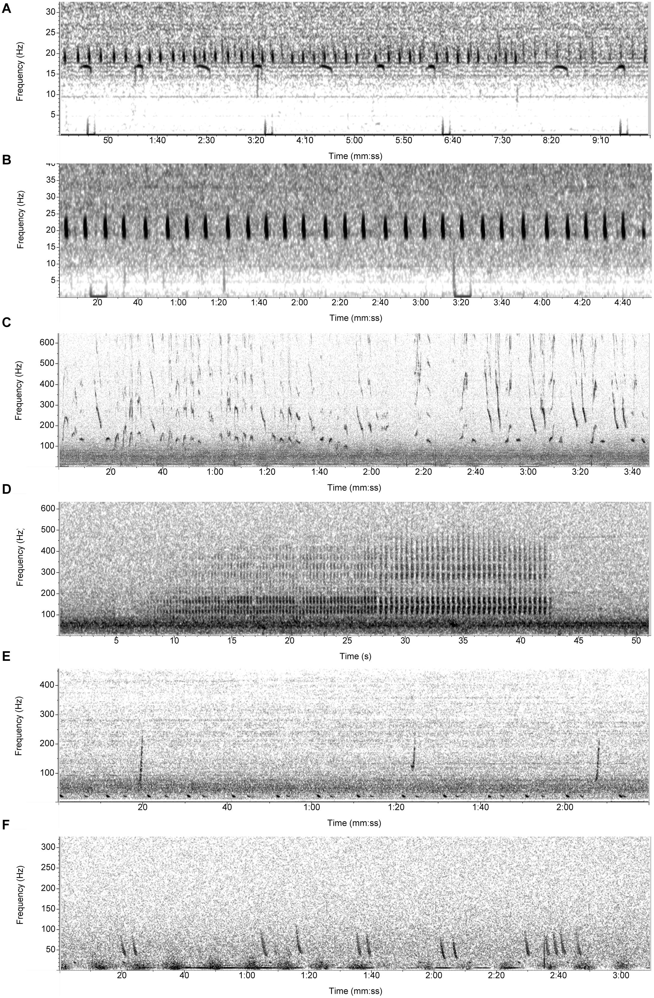
Figure 2. Spectrograms of the vocalization types used to detect species presence for the (A) blue whale (A/B song), (B) fin whale (20 Hz pulse), (C) humpback whale (song), (D) minke whale (pulse train), (E) North Atlantic right whale (upcall), and (F) sei whale (downsweep).

Low-frequency detection and classification system detections were manually reviewed by trained acoustic analysts to determine daily presence of each of the baleen whale species. Given the variability of each species’ vocalizations, the specific methodology to determine daily acoustic presence varied by species (see Davis et al., 2017, 2020 for a more complete description). A true detection was defined as a pitch track that correctly classified a call or song unit to the species that produced it (Bonnell et al., 2016). All detections were reviewed by an analyst until a true detection was found for NARW, sei, humpback, and blue whales. In contrast, only hours with 29 or more detections for fin whales were reviewed manually for acoustic presence due to a logistic regression application revealing 29 to be the minimum number of detections in an hour to ensure a fin whale was acoustically present with 90% confidence (Davis et al., 2020). This was implemented in order to reduce the time of manually reviewing detections. In addition, the automated pulse train detector which used a Ripple-Down Rule learner trained to identify the three main types of minke whale low-frequency pulse trains implemented by Risch et al. (2014), was applied to examine selected recordings for the acoustic presence of North Atlantic minke whales. It is important to note that the output from the classification model represents the relative daily proportion of species presence across 1-min clips while in our manual detection protocol, a day is marked as “present” for the full 24 h as soon as a single target species call type is observed. The manual detection protocol represents a minimum acoustic presence for each species in order to maximize confidence of acoustic presence. Therefore first, the model resolution presents information at a much finer scale than the latter approach and second, the output comparison between both methodologies concerns the period of the species-specific acoustic activity peak and its duration but not the magnitude of the daily activity or its monthly average.

Results

Species Richness of Training Data Set

All six baleen whale species were observed in the shelf training dataset for the random forest classification models, while only five target species were detected in the slope training dataset. Minke whale acoustic presence was only included in the analyses of the shelf dataset, and not the slope dataset due to the lack of minke whale vocalizations during the time periods analyzed when other baleen whale species were vocalizing in the slope dataset. Fin whales were the most represented species in the slope dataset, comprising just over 50% of the SR 1 clips. They were also the species most present in clips with the higher SR levels. NARW were present in the least number of clips in the slope dataset (27/695 clips). The shelf dataset had a more even representation of species in the clips than that of the slope dataset. The 1-min clips with SR of 0–2 co-occurring species were the most commonly observed in both training datasets (slope: 639/695 clips; shelf: 338/389 clips). The highest SR level found in the slope dataset was 3 (55/695 clips), and the highest in the shelf dataset was 4 (4/389 clips), indicating that most often 2 or fewer species were acoustically active at any given time and only rarely were there more than 2 species vocalizing.

Acoustic Metrics and Classification Models

The random forest classification models trained with a combination of relevant AM (Supplementary Table 1) showed high average accuracy values for all species around the slope and the shelf sites (Tables 2, 3). Overall model accuracy ranged between 80 and 92% for species around the slope site and between 82 and 95% for species around the shelf site. The false omission rate (class 0 error) was low for all species around both sites (0–12%), indicating that the models had high precision for predicting true species’ absence (Tables 2, 3). The classification models trained to discriminate the calls from the species around the slope site performed best for fin and right whales with false discovery rates (class 1 error) <0.15 (Table 2). However, model performance for blue, sei, and humpback whales was low (0.42, 0.54, 0.79, class 1 error respectively; Table 2). The precision of the classification models was higher in general for the species recorded around the shelf site, with false discovery rates (class 1 error) ranging from 0.43 (sei whales) to 0.12 (fin whales; Table 3). While the model’s ability to discriminate between SR levels was better for the shelf than the slope site (0.07 and 0.29 OOB errors respectively for SR 0), the model did not perform well at the higher SR levels for both sites in discriminating between the SR levels (Supplementary Table 2).

TABLE 2

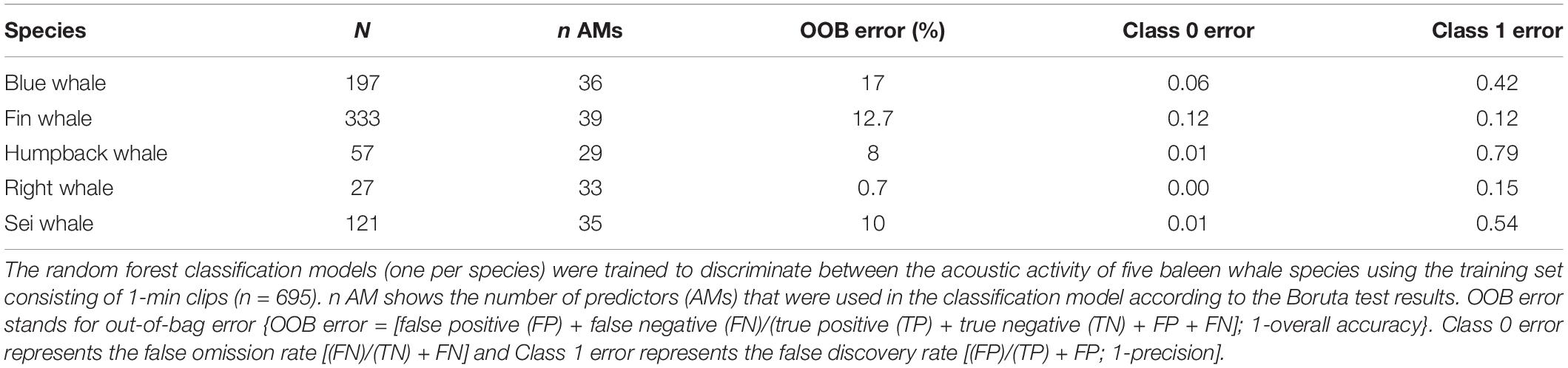
Table 2. Model results for the slope site.

TABLE 3

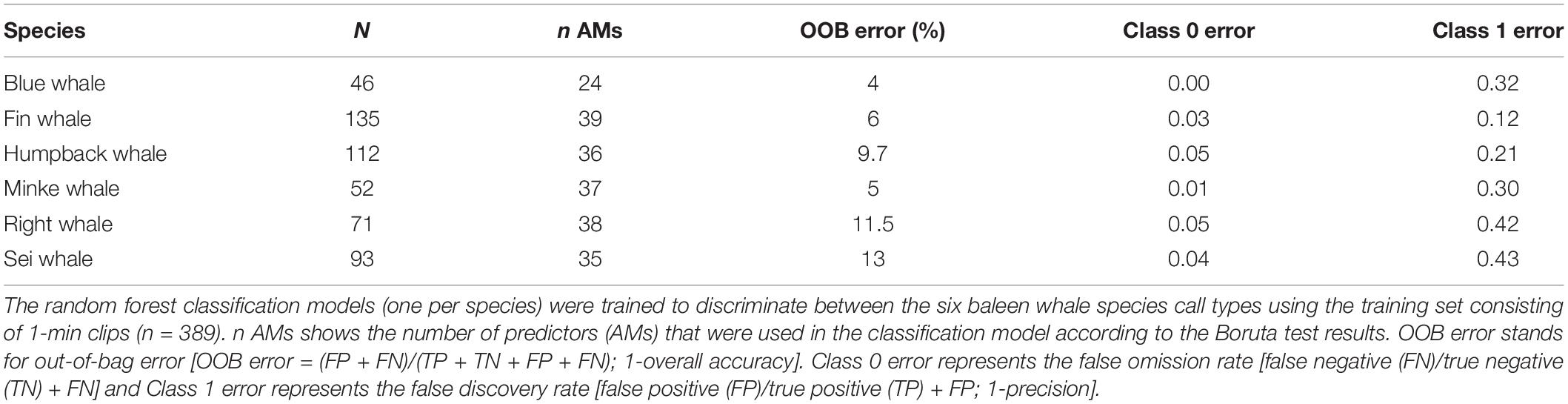
Table 3. Model results for the shelf site.

Figure 3 shows the relative importance of the different AM used in the random forest classification models to discriminate between the different species presence. The number of AM that were included in the classification models for species identification can be found in Tables 2, 3. Results on the conditional importance of the AMs used to train the classification models showed a good agreement in general between the AMs that were found to be most important for the classification of the different species acoustically present around the shelf and slope sites (Figure 3). Overall, the most important AMs were AMP, ACI, and BI (see Supplementary Table 1 for details). However, the importance of these AMs was highest when computed on the frequency bands corresponding with the bands in which the respective species’ call patterns show most of their acoustic energy (Figure 3). Further, there were also clear differences in the number of AM that were relatively most important between slope and shelf sites, with species in the latter being captured by a wider range of AM.

FIGURE 3

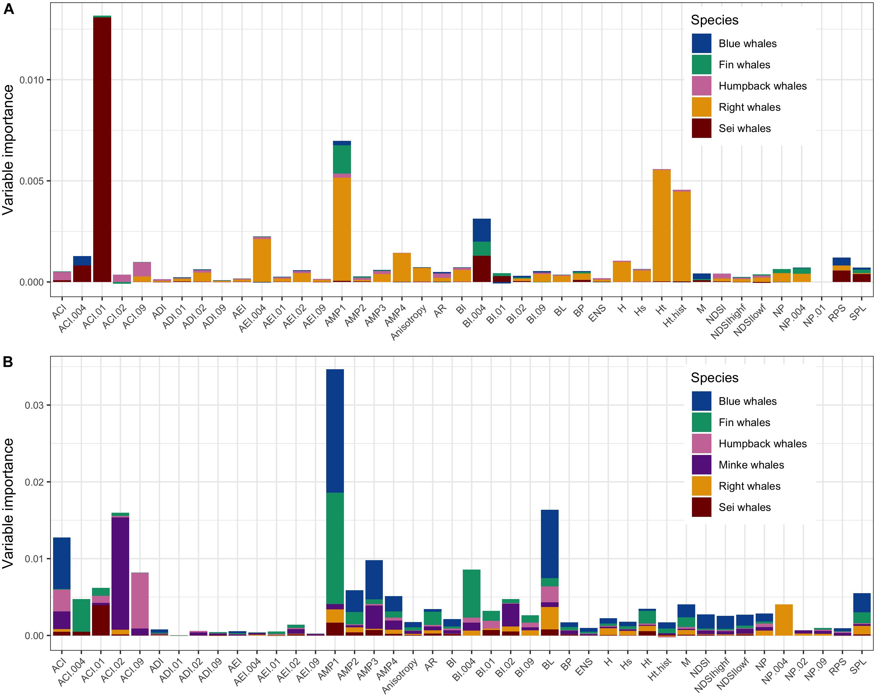
Figure 3. Conditional variable importance plot showing all AMs (predictors) included to train the random forest classification models and their relative importance per species. Top panel (A) represents the slope site, bottom panel (B) represents the shelf site.

Second-Step Model Evaluation of on Shelf Acoustic Recordings

The resulting model was applied to 12 months of near continuous acoustic recordings on the shelf site to evaluate its performance. Results on the second-step model evaluation showed high average accuracy scores for all species models regardless of the criteria used to determine the optimal threshold to produce presence/absence scores from the estimated probabilities. However, the threshold that in general yielded the best balance between sensitivity and precision for all species was the threshold that maximized Kappa (Table 4). The Kappa statistic provides a measure of agreement between the predicted and observed classes above that expected by chance (Kuhn and Johnson, 2013). Model performance was very high for fin, minke, and humpback whales with sensitivity and precision scores >0.70 (minke whale model precision = 0.67). Blue, NARW, and sei whales’ models showed high average accuracy and specificity but, in general, low sensitivity and precision (0.30–0.40; Table 4).

TABLE 4

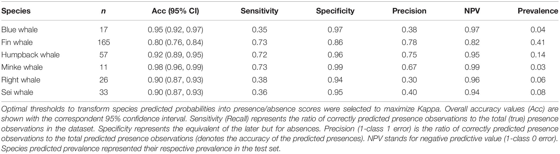
Table 4. Results on second-step evaluation of classification model performance on 14 months of acoustic data from the shelf site.

We then compared the long-trend output of the classification model to the results from the manual detection software approach that we standardly use to evaluate baleen whale presence in all of our western Atlantic data sets (Figure 4). The classification model estimation represents the species’ average daily relative presence proportion compared to a single verification of a species’ acoustic presence per day to determine daily presence in our manual detection methodology. Accordingly, the former provides much higher resolution detection information compared with the latter. The comparison made therefore is not between the raw proportion of presence in a given month (since the measures are not comparable) but in the timing and duration of the relative monthly acoustic presence peak for each species. The patterns in species presence showed good correspondence between the two methodologies for most species and time periods including peaks for blue whales in winter months, humpback, minke, and sei whales in spring months, and fin whales in late winter/early spring months (Figure 4). There were some discrepancies between the results of the model and manual verification. For example, fin whale proportion of acoustic occurrence showed higher proportions in the summer and fall months for the model approach, while fin whale presence showed zero proportion of acoustic occurrence during those same months in the detector and manual verification approach (Figure 4). Although the model did not perform well for blue and sei whale species when estimating acoustic presence at a 1-min clip level, when pooled across a day, the model provided a good approximation to the standard manual detection approach regarding the species relative presence and high activity periods.

FIGURE 4

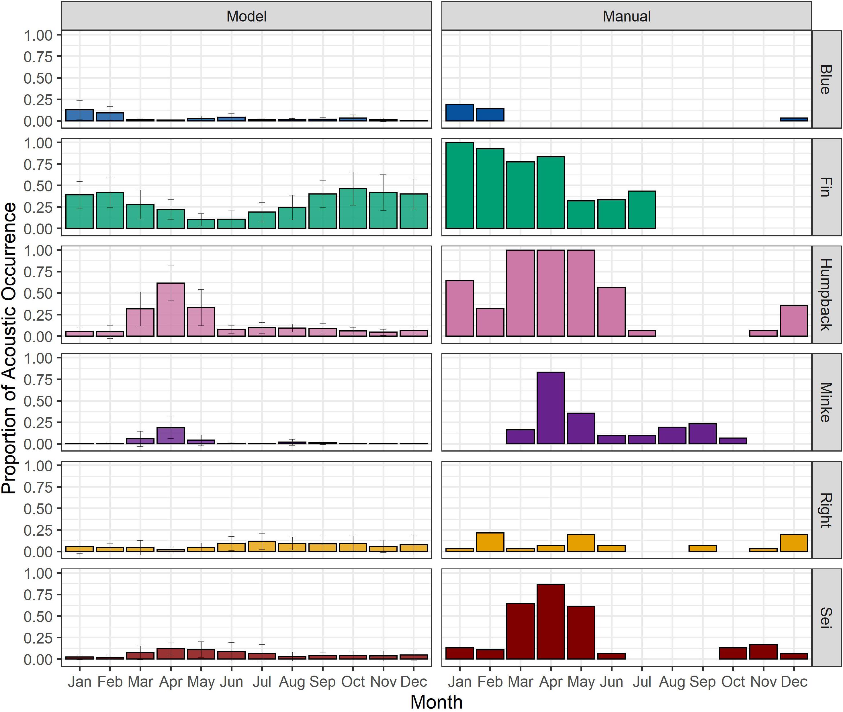
Figure 4. Relative daily proportion of acoustic presence (i.e., minutes per day/1,440 total minutes) estimated by the random forest classification models (left) and monthly proportion of acoustic presence (i.e., number of days present/total recording days in that month) found by manual review of automatic detections (right) for the species recorded at the shelf site over 12 months (January 1–December 31, 2017, with a gap from July 15 to 17, 2017). Color bars and correspondent error bars on the left panel (“Model”) show the monthly average (and ± SD) of the acoustic activity proportion predicted per species. The daily proportion of acoustic activity was computed as the relative proportion of the species presence scores obtained by applying the optimal threshold (Kappa criterium) to the estimated probabilities (left). Color bars on the right panel (“Manual”) show the number of days with confirmed acoustic presence over the number of total available recording months.

Discussion

This study showed that the shelf and slope sites include habitat that is utilized by the majority of baleen whale species that occur in the Northwestern Atlantic Ocean, with six and five different species detected at each site, respectively. However, in our training dataset, it was difficult to find more than two species vocalizing in the same 1-min time periods, resulting in low overall SR values. Due to the short length of the 1-min clips and the characteristics of the baleen whale calls around the study sites, it was not surprising that the SR levels were low in the clips analyzed. In some cases, different combinations of species’ vocalizations were detected at different times of day, or on nearby days, indicating that there were more species in the area than what may be represented by the SR values alone. Nevertheless, model discrimination for SR levels was poor (Supplementary Table 2), probably due to the higher intra- than inter-level acoustic variability, so it was not feasible to directly predict the number of co-occurring species in the same 1-min time period across the full datasets.

In this study, our random forest classification models trained with a combination of relevant AM were successful at discriminating the presence/absence of the call repertoire of different baleen whale species at the shelf and slope sites. Overall model accuracy was high for all species at both sites and in general, it was primarily driven by the model’s strong ability to predict the absence of the baleen whale species, meaning that they were highly successful at detecting time periods when specific species calls were not present. The false omission rate ranged from 0 to 5% on the shelf site, and 0 to 12% at the slope site, depending on species. Understanding when species are likely not to be acoustically present can be incredibly useful for marine soundscape planning, such as when trying to plan anthropogenic activities at times that could minimize acoustic disturbance to protected species (e.g., Van Opzeeland and Boebel, 2018). Being able to predict a species acoustic absence using rapid techniques can facilitate more efficient processing of large datasets.

At the shelf and slope sites, the models were also successful at predicting presence for a subset of our target species. The models performed the best for fin whales, predicting their presence with an 88% precision at both sites. This is similar performance to that reported for fin whale detectors in other studies (e.g., Buchan et al., 2019; Fregosi et al., 2020). The model also performed well for NARW at the slope site (15% false discovery rate) and humpback whales at the shelf site (21% false discovery rate). However, the ability to accurately predict presence decreased for the other species/site combinations, with false discovery rates ranging from 30 to 79%. In general, the random forest classification models performed somewhat better on the shallower shelf site as compared to the deep-water slope site. This may be due to a combination of differences in ambient noise backgrounds, propagation influence at the slope site based on hydrophone depth, as well as overall species occurrence. While the false discovery rates were lower for the shelf site than the slope site for blue, humpback, and sei whales, the model had a higher false discovery rate at the shelf site for NARW than the slope site. This could be attributed to the quality of signal in the NARW clips in the slope site even though they were only acoustically present in around 4% of the slope clips. The low SR and minimum amount of overlap between target signals may well have improved our model performance in some instances. Our North Atlantic sites may be considered less “acoustically cluttered” compared with tropical waters; we did not have to contend with issues such as fish chorusing and snapping shrimp as previous studies did (e.g., Buxton et al., 2018). However, instead our region is subject to high anthropogenic noise levels (Rice et al., 2014), which impacted our model performance for species like humpback whales whose variety of vocalizations clearly overlap the same frequency ranges.

In our dataset, the metrics that contributed the most to species classification were those that summarized acoustic activity (intensity) and complexity in different frequency bands, such as AMP and ACI. In particular, important contributors to model performance were the AM computed across the lower frequency bands corresponding with the bands in which the respective species’ call patterns show most of their acoustic energy (Table 3). Furthermore, for specific species/sites combinations, BI, Ht, and BL (see Supplementary Table 1 for details) also showed high relative importance suggesting that the acoustic spectral and temporal heterogeneity, together with the background noise level were important drivers in the discrimination process between the species acoustic presence/absence. While it is interesting to note the relative importance of these AMs within the species-specific models, in the current study, the AMs are merely an automated way to parameterize and train the model when combined all together.

The role of acoustic indices, and AM in general, is essential to quantify the complexity of the soundscape in a single or handful of values. However, their success has been variable, and it seems that a combination of AM (rather than a single metric) is more effective at predicting bioacoustic activity (Sueur and Farina, 2015; Mooney et al., 2020). Drawing from our results, the utility of these metrics may well reflect and capture the complexity and stereotypy of individual species call types with NARWs and sei whales generally producing sporadic bouts of calls, while fin, blue, and minke whales produce song sequences which are more frequent and longer in duration (Figure 2; e.g., Stafford et al., 2007; Risch et al., 2014; Cholewiak et al., 2018; Davis et al., 2017, 2020). In noisy, shallower waters where snapping shrimp choruses also dominate, the soundscape can be homogenized because of the wide frequency range, pervasiveness, and intensity of this characteristic sound. This acoustic context may challenge the use of AMs to train classification models to discriminate other concurring calls (e.g., fish). In contrast, acoustic contexts dominated by whale calls, or even song, as the ones studied at these sites, generally have a narrower band and less intense background and therefore, they may provide a promising route for using AM or an adapted version thereof as was shown in Parks et al. (2014).

Second-step evaluation of model performance in new data showed relatively high performance for three species: fin, humpback, and minke whales (Table 4). For these species, the model performed well in predicting species presence as well as absence, similarly to the results of the first stage analysis. Overall predicted prevalence in the dataset for these three species ranged from 41% (fin whales) to 3% (minke whales; Table 4). However, the model performed worse for blue, NARW, and sei whales when applied to the entire dataset, with low rates of precision and sensitivity.

The comparison between model and detector outputs was aimed at understanding how the trained model would perform across a long time series (12 months of data), and whether it would provide outcomes that were comparable to the results obtained from the more time-consuming acoustic detection software approaches. When we averaged the model predictions and compared to the average daily presence across each month, the model predicted clear seasonal patterns of occurrence for all species well (Figure 4). In comparison to our standard acoustic detection software process, the model provided much finer resolution and increased presence information. It is important to remember that the model provided information on species presence at the resolution of 1-min clips, while our standard acoustic detection approach provided species presence at the resolution of 24 h (daily). Therefore, although the model performed poorly when predicting certain species presence at the 1-min clip level, when aggregated across a day, it predicted similar patterns of occurrence as our standard acoustic detection software approach. However, there were time periods where the model accurately showed a larger proportion of daily acoustic presence for some species than the detector, like for fin whales during the summer and fall in 2017. Some of the discrepancies between the two methodologies could be explained by the missed detection rates of the detectors and the constrains of the manual verification process used (see section “Model Predictions and Second-Step Evaluation”). As mentioned in section “Model Predictions and Second-Step Evaluation”, the detector methodologies were aimed at determining species’ minimum acoustic presence. False negative rates for humpback, blue, fin, and sei whales were found to be 5, 10, 10, and 14%, respectively (Davis et al., 2020). Davis et al. (2017) found 31% of days where NARW were acoustically present were missed by the LFDCS detector. Lastly, the minke whale pulse train detector was found to have a 27% false negative rate (Risch et al., 2013). Because of these slight discrepancies, a detector method could be used in instances where the results aim to be more conservative, and species presence should be manually verified. In contrast, the AMs classification model can provide accurate species absence and presence information at daily-scale resolution with minimal human verification of the models’ predictions. This demonstrates that this approach is valuable at this coarser reporting level.

Where the AM methodology really came into its own was both in the reduction of time needed to process large quantities of data by reducing the processing time from days to hours. In addition, the increased detection resolution that the AM model provides allows for a much more in-depth analyses of the data, allowing for tidal and diel trends to be evaluated in addition to having much finer resolution on species presence. The acoustic detector currently provides a manageable but time consuming and coarse resolution of information. Further improvements to this model are likely possible by adding higher resolution clips and more training data aimed at improving the positive detection accuracy and decreasing false detections. Also, in areas where the model and manual detector methods showed differing species presence proportions, clips could be browsed from those areas to confirm or deny species presence to further inform the model’s test training datasets. However, results show that this methodology has promise to stand as an alternative or complementary analysis to current methods used for understanding large scale daily distribution of baleen whale species.

Overall, a relevant combination of AM in the context of a random forest classification modeling approach provides a promising methodology for less time consuming and laborious species detection for baleen whales based on the AM processes taking half as long as manually reviewing the detectors for these two sites. In addition, it could equally provide significantly higher resolution of information than what is currently available. Passive acoustic monitoring in the marine environment continues to rapidly expand as a methodology for understanding species occupancy and distributions to avoid human impacts and understand changing ocean environments for these species (e.g., Van Parijs et al., 2009; Mann, 2012; Rettig et al., 2013; Wall et al., 2013). With the end user in mind (Mooney et al., 2020) further development of this type of multi-step evaluation of AM could provide highly valuable advances in speed and improved resolution of data extraction.

Data Availability Statement

The raw data supporting the conclusions of this article will be made available by the authors, without undue reservation.

Author Contributions

SV, DC, NP, and IR contributed to the conception of the study and wrote sections of the manuscript. SV and DC provided project management. NP and GD performed analysis of acoustic data. IR completed computing of acoustic metrics and random forest classification models. IR and GD created the figures. All authors contributed to editing the manuscript and approved the submitted version.

Funding

The data collected and analyses conducted in this project for the slope site were funded by Joel Bell through the United States Fleet Forces Command and managed by Naval Facilities Engineering Service Command Atlantic under the United States Navy’s Marine Species Monitoring Program and for the shelf site by Bureau of Ocean and Energy Management (BOEM) Atlantic Marine Assessment Program for Protected Species (AMAPPS) program.

Conflict of Interest

The authors declare that the research was conducted in the absence of any commercial or financial relationships that could be construed as a potential conflict of interest.

Publisher’s Note

All claims expressed in this article are solely those of the authors and do not necessarily represent those of their affiliated organizations, or those of the publisher, the editors and the reviewers. Any product that may be evaluated in this article, or claim that may be made by its manufacturer, is not guaranteed or endorsed by the publisher.

Acknowledgments

We thank Liam Mueller-Brennan, Timothy Rowell, Tyler Aldrich, and the Passive Acoustics Group at NEFSC for their assistance and contributions to the data analyses. We thank Ilse Van Opzeeland for contributions to the study design and implementation. We also thank the Cornell Center for Conservation Bioacoustics and the Scripps Whale Acoustics Laboratory for their previous assistance with the data collection and extraction.

Supplementary Material

The Supplementary Material for this article can be found online at: https://www.frontiersin.org/articles/10.3389/fmars.2021.749802/full#supplementary-material

Footnotes

^ www.benthos.com

References

Baumgartner, M. F., and Mussoline, S. E. (2011). A generalized baleen whale call detection and classification system. J. Acoust. Soc. Am. 129, 2889–2902. doi: 10.1121/1.3562166