A Clustering Approach for Predicting Dune Morphodynamic Response to Storms Using Typological Coastal Profiles: A Case Study at the Dutch Coast

Dune erosion driven by extreme marine storms can damage local infrastructure or ecosystems and affect the long-term flood safety of the hinterland. These storms typically affect long stretches (∼100 km) of sandy coastlines with variable topo-bathymetries. The large spatial scale makes it computationally challenging for process-based morphological models to be used for predicting dune erosion in early warning systems or probabilistic assessments. To alleviate this, we take a first step to enable efficient estimation of dune erosion using the Dutch coast as a case study, due to the availability of a large topo-bathymetric dataset. Using clustering techniques, we reduce 1,430 elevation profiles in this dataset to a set of typological coastal profiles (TCPs), that can be employed to represent dune erosion dynamics along the whole coast. To do so, we use the topo-bathymetric profiles and historic offshore wave and water level conditions, along with simulations of dune erosion for a number of representative storms to characterize each profile. First, we identify the most important drivers of dune erosion variability at the Dutch coast, which are identified as the pre-storm beach geometry, nearshore slope, tidal level and profile orientation. Then using clustering methods, we produce various sets of TCPs, and we test how well they represent dune morphodynamics by cross-validation on the basis of a benchmark set of dune erosion simulations. We find good prediction skill (0.83) with 100 TCPs, representing a 93% input and associated computational costs reduction. These TCPs can be used in a probabilistic model forced with a range of offshore storm conditions, enabling national scale coastal risk assessments. Additionally, the presented techniques could be used in a global context, utilizing elevation data from diverse sandy coastlines to obtain a first order prediction of dune erosion around the world.

Introduction

Coastal storms erode sandy beaches and dunes (Vellinga, 1982; McCall et al., 2010; Castelle et al., 2015; Masselink et al., 2016; Harley et al., 2017) with direct impacts on coastal communities through damages to developments and infrastructure (Jongejan et al., 2016; Ballesteros et al., 2018), reduction of beach’s touristic and recreational value (Monioudi et al., 2017; Toimil et al., 2018), and disturbance of coastal ecosystems (Mehvar et al., 2018; Paprotny et al., 2021). Moreover, the beach and dune system forms the first line of defense against coastal flooding, and their weakening or breaching can worsen the hinterland’s susceptibility to flooding (Grzegorzewski et al., 2011; Keijsers et al., 2015; van Dongeren et al., 2018; Almar et al., 2021).

As coastal change predictions are critical for coastal zone management and decision making, process-based numerical models have been developed and used extensively in order to simulate morphological changes at the dune system during extreme events (Roelvink et al., 2009; McCall et al., 2010; van Dongeren et al., 2018). However, these models can be computationally expensive, especially when the spatial scale of interest is large (∼100s of km), or a large range of boundary conditions need to be applied. Computational time is, for example, of great importance in early warning systems, when the forecast window is limited, or in probabilistic projections when a large number of simulations are needed (Ranasinghe et al., 2012).

Conventionally, forecasts and assessments are performed on individual profiles because the intensity of large-scale erosion is not only associated with the offshore characteristics of a storm event such as the maximum storm surge, maximum wave height and duration, but also on pre-storm dune and foreshore morphology and their interactions with the forcing (Houser et al., 2008; Masselink et al., 2016; Athanasiou et al., 2018; Davidson et al., 2020). Exploration and understanding of these dependencies require the availability of high-quality observations of coastal change with pre- and post-storm surveys over large coastal areas, which are quite challenging to obtain. Only some recent studies started to explore the controls of this spatial variability in coastal response using such datasets. For example, Beuzen et al. (2019) used a unique dataset of around 1,700 pre- and post-storm cross-shore profile transects covering a 400 km span along the southeast Australian coastline, to understand beach and dune erosion variability. The authors found different controls responsible for the erosion of the beach and dune system, where the dune response was governed by the local beach width and wave runup and beach response was linked to pre-storm beach volume. Cohn et al. (2019), employed both observations along the United States Pacific northwest coast and simulations using the process-based model Xbeach (Roelvink et al., 2009) with schematized coastal profiles to study the influence of pre-storm morphology and environmental conditions (i.e., wave forcing and water levels) on dune erosion, finding strong controls in backshore beach slope, nearshore slope and the dune slope.

In recent years, predictive tools or meta-models that employ large number of observations or usually simulations along with statistical techniques (e.g., Bayesian Networks), have shown potential for producing efficient predictions of coastal hazard indicators (Gutierrez et al., 2011; Poelhekke et al., 2016; Beuzen et al., 2017; Pearson et al., 2017; Giardino et al., 2019; Rueda et al., 2019; Santos et al., 2019; Sanuy and Jiménez, 2021). The concept underlying these meta-models is the use of a large number of combinations of forcing conditions and/or coastal elevation profiles to predict coastal response. This type of generic tools can be used in first-pass coastal impact assessments or early warning systems to identify hotspots along the coastline (Viavattene et al., 2017; van Dongeren et al., 2018). These models are trained with model-generated coastal hazard datasets due to the general lack of observations during extreme events, while the choice of the input parameters must ensure generalization of the model to avoid overfitting (Beuzen et al., 2018). Input reduction is of critical importance when applying these approaches, as it decreases the computational constrains of creating the synthetic dataset without significantly affecting the prediction skill.

Input reduction in coastal applications has been commonly applied to reduce model forcing (Walstra et al., 2013; Chiri et al., 2019; de Queiroz et al., 2019) for long-term morphodynamic cases. Recently, Scott et al. (2020) presented a methodology to reduce a large dataset (>30,000) of coral reef topo-bathymetric profiles to a representative subset (on the basis of wave runup) of 50–312 profiles, using machine learning, statistics and a numerical model. Using clustering algorithms to obtain the representative profiles and a probabilistic matching technique, they predicted wave runup for a test subset of profiles with a mean error of 9.7–13.1%, highlighting the potential of these techniques. Alternatives for capturing the variability in topo-bathymetric characteristics, such as the creation of schematic cross-shore profiles based on a set of parameters (Pearson et al., 2017; Cohn et al., 2019), lack the realistic representation of the actual coastal features and can be computationally infeasible, since adding parameters and/or increasing their resolution can increase the number of simulations exponentially (Scott et al., 2020).

The main aim of this study is to explore whether a selected number of coastal profiles along a ∼100 km coastline is representative of the expected variability of the dune morphodynamic response during extreme events over the whole coastline. This would reduce the number of simulations needed to characterize storm impacts over the whole system and ultimately aid in having more efficient prediction tools at large spatial scales.

Here we built upon Scott et al. (2020), with a focus on sandy coasts and dune erosion. Our case study is the Dutch coast where dune erosion is of critical importance for coastal zone management, with the dune system being the first line of defense against coastal flooding (de Vries et al., 2012) of the low-lying hinterland which is below mean sea level at almost one quarter of the country (Schiermeier, 2010). To that end, the unique regional scale topo-bathymetric profiles dataset JARKUS (Rijkswaterstaat, 2018) is available for the entire Dutch coast. We used this dataset together with offshore wave/water level observations to obtain a number of morphological and hydrodynamic parameters for each profile along the Dutch coast. Additionally, we employed the process-based numerical model Xbeach (Roelvink et al., 2009) to characterize the profiles on the basis of dune erosion volumes during extreme events, exploring dependencies of simulated spatial variabilities. Combining these data with clustering algorithms, we reduced the total profiles to a representative subset of profiles, which we refer to as Typological Coastal Profiles (TCPs), after first exploring the dependencies and relative importance of the derived profile parameters. Subsequently we assessed the effectiveness of the proposed technique by using the developed TCPs to predict dune erosion for an arbitrary set of test profiles. The proposed methodology can be applied at other areas with sandy beach and dune systems globally and ultimately may facilitate the development of large-scale dune erosion prediction tools (Viavattene et al., 2017).

Section “Materials and Methods” describes the methods used in the present study to obtain the profile characteristics, simulate dune response and to cluster the profiles. Results are presented in section “Results.” In section “Discussion” a discussion on the insights obtained in the present study, the limitations of the presented methodology and its implications for applications elsewhere is presented. Ultimately, a summary of the main conclusions of the work herein can be found in section “Conclusion.”

Materials and Methods

An outline of the methodology used in the present study is shown in Figure 1. The objective is to reduce a set of 1,430 cross-shore elevations profiles along the Dutch coastline from the JARKUS dataset to a, still representative, smaller number (M) of TCPs, which can then be used in large scale, probabilistic prediction tools or impact assessments. First the available data, including the input cross-shore profiles and wave and water level observations, are described (section “Case Study and Data Availability”). Then, from these datasets, morphological (section “Morphological Parameters”) and hydrodynamic (section “Hydrodynamic Parameters”) parameters are derived using simple calculations to characterize each profile in the JARKUS dataset. Next, 10 representative storm boundary conditions are obtained from the offshore observations (section “Representative Offshore Storms”). A benchmark dataset on dune erosion volumes is developed by modeling the impact of these 10 representative storms on the original JARKUS profile dataset with XBeach (section “Dune Erosion Modeling and Indicators”). Subsequently, the clustering approach that was considered herein to attain the TCPs is demonstrated (section “Clustering of Coastal Profiles”). Finally, the use of the produced TCPs to obtain dune erosion predictions for a sample of test profiles is described and the evaluation of the skill of each clustering technique considered is assessed (section “Prediction and Validation”).

FIGURE 1

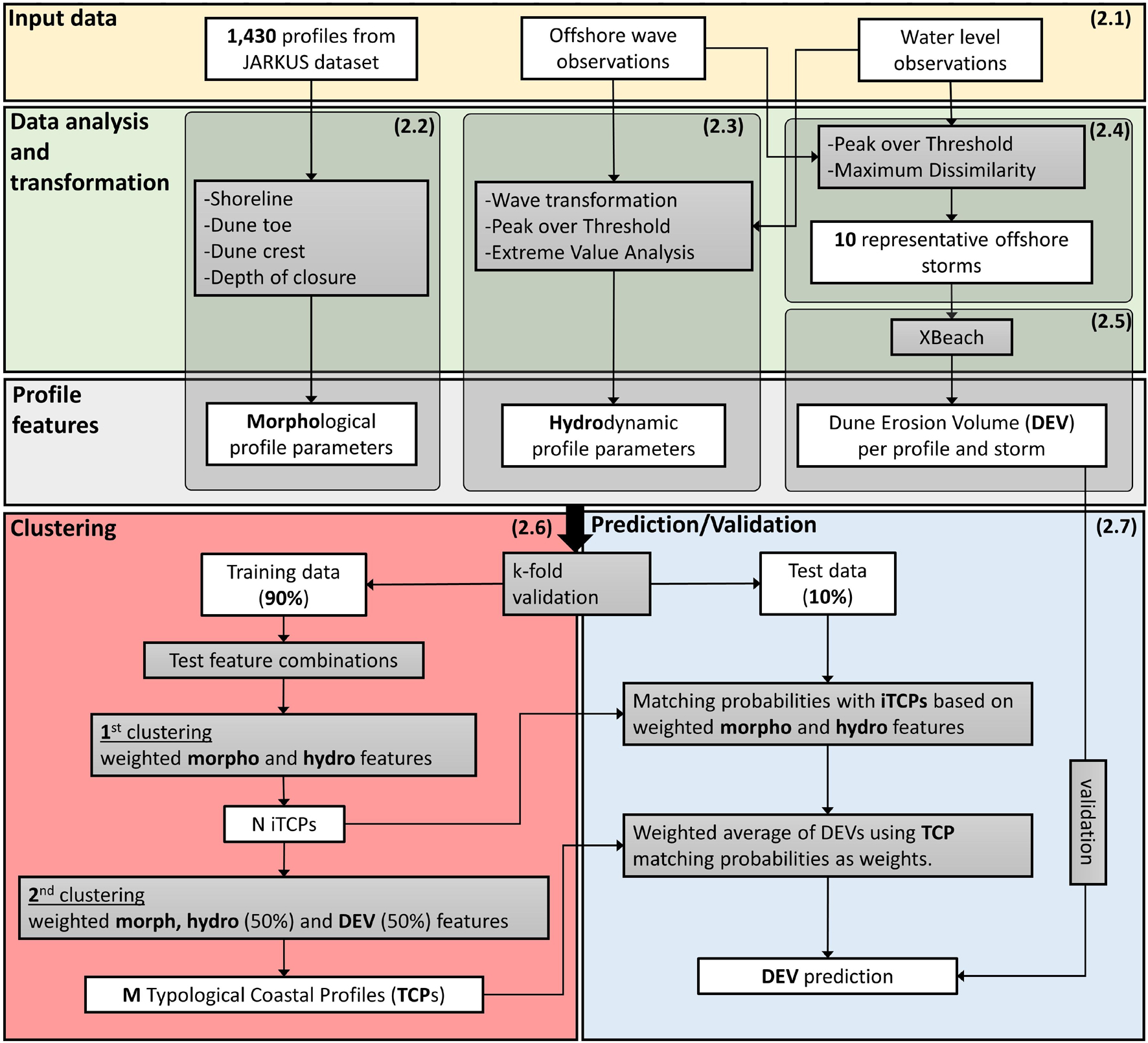
Figure 1. Flow diagram of the methodology followed in the present study to reduce the initial dataset of Dutch coastal profiles to M typological coastal profiles (TCPs), based on their morphological, hydrodynamic and dune erosion characteristics, which were calculated using various observations, data analysis and modeling. The extracted TCPs were used to make predictions of dune erosion volume (DEV) for a set of test profiles using the simulated DEV as benchmark for the validation. Parentheses in top right corners of boxes indicate the section number that each part is described in.

Case Study and Data Availability

The Dutch coast is located at the North Sea, has a length of about 432 km and can be divided in three regions: (1) the Delta region in the South which is formed by islands and estuaries, (2) the Holland coast in the center, which is characterized by long sandy beach and dune systems and (3) the Wadden islands in the North, comprising barrier islands and tidal inlets (Figure 2). Of the 432 km of coastline, 254 km comprise beach and dune systems (Ruessink and Jeuken, 2002), the majority of which are affected by human interventions (by means of nourishments, planting etc.) (Arens and Wiersma, 1994). As part of the JARKUS (“Jaarlijkse Kustmeting,” Annual Coastal Measurement) program, depth and elevation measurements are performed annually (between April and September) at fixed transects along the Dutch coast with a temporal coverage dating back to 1965. Elevation is measured with respect to the NAP (“Normaal Amsterdams Peil”), which is the national vertical datum and roughly corresponds to mean sea level (MSL). Depending on the time and region, these transects have an alongshore interval of ∼250 m to ∼1 km and a cross-shore resolution of 5 and 10 m for the sub-aerial and sub-aqueous parts, respectively. From the 2,285 available transects, 1,430 sandy transects were chosen for the present study (Figure 2), after excluding transects where surveys no longer take place at 2019 (year of the study) and transects that are not beach-dune systems. This filtering was performed by visual inspection, excluding areas that have non-erodible hard structures or transects at highly dynamic areas with no distinct dune features (i.e., inlets at Wadden islands). The measurements of the latest year at the time of the study (2019) were used as the pre-storm profiles in the present analysis.

FIGURE 2

Figure 2. Map of the Dutch coast, indicating the location of the JARKUS transects, wave buoys and tide gauges used in the present study. Transect 7002882, appearing in Figure 3, is highlighted in purple. The map is projected on the “Amersfoort / RD new” coordinate system with the X and Y axis in meters. Basemap obtained from ESRI (2011).

Time series of wave parameters at a 3-hourly resolution were available between 1979 and 2009 from directional wave-riders, at four offshore locations at depths of 32, 21, 26, and 19 m for the measurement’s locations from South to North, respectively (Figure 2). This included significant wave height (H_s,₀), peak wave period (T_p,₀) and mean direction (Dir₀). Additionally, water level time-series at a 10 min interval were available from four tide-gauges along the Dutch coast (Figure 2), from which local tide and storm surge level (SSL) were obtained by performing a tidal analysis with the T_Tide package (Pawlowicz et al., 2002). These data were available from Rijkswaterstaat, an agency of the Ministry of Infrastructure and Water Management of the Netherlands.

Morphological Parameters

For each profile, a set of morphological pre-storm parameters was calculated using the JARKUS elevation profiles of 2019. First, the location of the maximum dune crest, foredune crest, dune toe, MSL point and depth of closure were detected. The maximum (i.e., highest) dune (from now on referred to as max dune) crest location was defined as the location of the maximum elevation across the profile. The foredune crest was identified as the most seaward elevation peak, with a minimum elevation of 7 m, a minimum width of 5 m and a minimum seaward prominence of 2 m. These additional thresholds, which are necessary to ensure that low elevation undulations on the beach were not detected erroneously as the foredune, were determined by performing a sensitivity analysis on the threshold values and visual inspection using satellite imagery. The dune toe location was calculated using the approach of Diamantidou et al. (2020), by finding the location of the most seaward crossing of a threshold of 0.01 for the 2nd derivative of the elevation profile (smoothed with a Hanning window of 20 m), between the foredune crest and the local mean high water (MHW) point, in the 1–5 m elevation range. The MSL profile point was identified by the most seaward intersection of the elevation profile with the 0 m elevation line (assumed to be at 0 m NAP level). The depth of closure point was found by the most landward intersection of the elevation profile with the elevation of the local depth of closure as extracted from the closest points in the global dataset of Athanasiou et al. (2019). These five points defined four areas along each profile: (1) The max dune area, between the max dune crest and the dune toe, (2) the foredune area, between the foredune crest and the dune toe, (3) the beach area, between the dune toe and the MSL point and (4) the nearshore area, between the MSL point and the depth of closure (Figure 3).

FIGURE 3

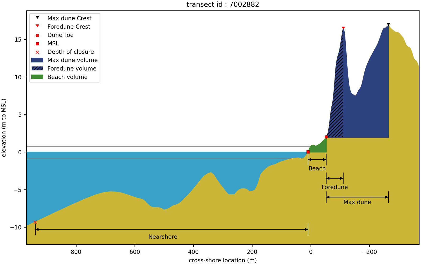
Figure 3. Example of cross-shore elevation profile and morphological locations and areas for one transect (Transect 7002882 – see Figure 2 for location) along the Dutch coast. The black lines around the MSL line (blue hatch) indicate the elevation of the MLW and MHW. Volumes indicated are volumes per meter alongshore.

Subsequently, using the aforementioned areas, a set of geometric parameters of the dune, beach and nearshore areas were derived to characterize each profile. The choice of these morphological parameters was based on previous studies that have associated such parameters with dune erosion variability (Beuzen et al., 2019; Cohn et al., 2019). First, the elevations of the max dune crest, foredune crest, and dune toe were extracted. Then the max dune (foredune) volume was calculated as the subaerial sand volume, per alongshore running meter, seaward of the max dune (foredune) crest and above the dune toe elevation. The max dune (foredune) width was calculated as the cross-shore distance between the max dune (foredune) crest and the dune toe. The max dune (foredune) volumes and widths, as calculated here, actually represent the half – volumes and widths. The beach width and volume were defined between the dune toe and above the MSL point. Additionally, slope parameters were calculated for the foredune, beach and nearshore areas as the linear slope between the two endpoints of each section, as previously defined (Figure 3). The intertidal slope was calculated as well, between the MHW and mean low water (MLW) points (derived from the local water levels defined in the JARKUS dataset). All these morphological parameters describe the pre-storm profiles hereon.

The foredune crest elevation has a high spatial variability with values between 7.7 and 21.3 m (5th–95th percentiles), and a median of 13.3 m (Supplementary Figure 1). The highest elevations appear in the center of the Holland coast, while values are lower for some of the Wadden coast and most of the Delta coast. The distribution of the beach width follows a more one-tailed distribution with extremes appearing in some areas with extended beach features, mostly as a result of beach nourishments (e.g., the Sand Motor mega-nourishment in the south part of the Holland coast) and has a median value of 71 m. The beach volume is highly correlated with the beach width, having same spatial patterns and a median value of 146 m³/m. Most of the coastal profiles have relatively mild nearshore slopes with a median value of 0.008, with steeper slopes appearing mainly in areas where tidal inlets are encountered (e.g., southern Delta coast and island corners at Wadden coast).

Hydrodynamic Parameters

Besides the morphological characterization of the coastline presented in the previous section, there are variabilities in the hydrodynamics along the Dutch coast that can affect the dune response during extreme events. For example, the local tidal amplitude may influence the total water levels and thus dune erosion directly, and the profile orientation may dictate the local profile exposure to specific storm conditions. On the other hand, spatial variabilities in wave conditions can implicitly shape local profiles, information which might not be always captured in the previously defined morphological parameters. To this end, a set of hydrodynamic parameters was produced for each profile, in order to test their influence on dune response variability.

In order to characterize the local hydrodynamic environment of each profile, the offshore wave time-series (H_s,₀, T_p,₀, and Dir₀) from the closest wave buoy (accounting for the geophysical extents of each area as well, see Figure 2) were transformed to the local depth of closure (H_s, T_p, and Dir) using a simple linear transformation and Snell’s law, assuming alongshore uniform bathymetry. Subsequently, a peak over threshold (POT) technique was applied on the local time-series of H_s to identify extreme events in the historical period between 1979 and 2009 for each profile. An event was defined, between an up-crossing and down-crossing of a chosen H_s threshold, with a minimum separation between events of 24 h, and a minimum event duration of 6 h (Wahl et al., 2016). The H_s threshold of each profile was chosen to have an average of five events per year (i.e., ∼150 events in record). For each event, the maximum H_s and SSL, and the concurrent T_p and Dir were extracted. The average angle of incidence during the historic extreme events (a_{extreme,  mean}) and the average wave energy flux toward the coast (P_{x  extreme,  mean}) (Harley et al., 2017) were calculated at each location. The MHW of each profile was extracted from the JARKUS dataset. Thereafter, an extreme value analysis (EVA) was performed on H_s, SSL, and T_p. A generalized Pareto distribution was fitted to the extreme H_s, while for T_p and SSL, the best fit distribution was chosen from a set of typical distribution used in coastal applications (generalized extreme value, exponential, gamma, inverse Gaussian, logistic, lognormal, Rayleigh, and Weibull), by minimizing the root mean square error (RMSE) between the theoretical and empirical non-exceedance probabilities (Wahl et al., 2016). Then extreme values for each parameter with various return periods (RP) could be extracted for each profile. Here the 100 years RP is used as a representative extreme probability (i.e., one that could result in significant dune erosion) to get the associated H_s,_RP100, T_p,_RP100, and SSL_RP100 for each profile.

The local extreme wave statistics (H_s,_RP100, T_p,_RP100, and SSL_RP100) show significant variability with increasing (e.g., more severe) values from south to north (Supplementary Figure 2). Their median values along the Dutch coast are 8.8 m, 15 s and 2.5 m, respectively. The MHW (i.e., tidal amplitude) increases from south (∼ 0.7 m) to north (∼1.7 m) as well. The average angle of incidence of the historic extreme events a_{extreme,  mean} per profile have mostly values between -28° and 10° (5th and 95th percentile, respectively) and has a median of 0.6° (i.e., almost shore normal). This parameter is an indicator of the individual profile orientation and the local wave climate. Generally, extreme storms seem to arrive relatively normal to the shore at the Holland coast, while they arrive at an angle at the Wadden and Delta coasts. The average wave energy flux toward the coast of the historic events P_{x  extreme,  mean} is a combination of the H_s and the profile orientation. It generally has lower values along the Delta coast compared to the Wadden coast due to local profiles orientation and variations in H_s, and has a median value of 190 KWh/m along the entire Dutch coast.

Representative Offshore Storms

Since pre-storm and post-storm surveys of coastal elevations were not available at the spatial scale of this study, representative storms from the historic offshore records and a process-based model were used to simulate the impact of extreme storm events on the dune system (section “Dune Erosion Modeling and Indicators”). The spatial variation of the morphodynamic dune response was then utilized to identify dune erosion drivers, to group profiles with similar responses and as a benchmark for validating the proposed clustering techniques.

Here extreme events were identified at time instances when H_s,₀ and SSL are both high, making it more likely that dune erosion will occur. Previously, Li et al. (2014), have used thresholds of 3 and 0.5 m, for H_s,₀ and SSL, respectively, for identifying extreme events with dune erosion potential at the IJmuiden-06 location at the Holland coast (Figure 2). After testing these values, it was found that for a high number of the detected storms the dune erosion was minor for most of the Dutch profiles, so the thresholds herein were increased to 5 and 1.5 m, respectively, to make sure that only events with relatively substantial dune erosion potential were included. The approach that was followed to identify the observed extreme storms and their characteristics comprised: (1) finding the H_s,₀ exceedances of the threshold of 5 m in the H_s,₀ time-series; (2) defining the duration (D) of the event as the time period when H_s,₀ remained above this threshold, while events with a time separation of less than 24 h were merged as they were assumed to be associated with the same storm (Wahl et al., 2016); (3) extracting the maximum H_s,₀ during the event, and the concurrent T_p,₀ and Dir₀; (4) extracting the maximum SSL during the event; (5) excluding events with a maximum SSL less than 1.5 m. These steps were applied to the records of all four offshore stations (Figure 2) to make sure that the spatial variability in the offshore wave climate was accounted for, creating a database of 70 storm events with their descriptive parameters (H_s,₀, T_p,₀, DIR₀, SSL, and D). Then, the Maximum Dissimilarity Algorithm (MDA) (Camus et al., 2011) was applied to choose a subset of 10 representative events, which were the most dissimilar (defined by Euclidean distances in the parameter space) with respect to their storm parameters (Figure 4 and Table 1). The most dissimilar event (i.e., the one with the highest sum of Euclidean distances to all other events) was used as the seed (i.e., the initial data of the subset) in the MDA. The number of storms was chosen in order to ensure that the storm variables space was sampled sufficiently, while maintaining computational costs at a feasible level.

FIGURE 4

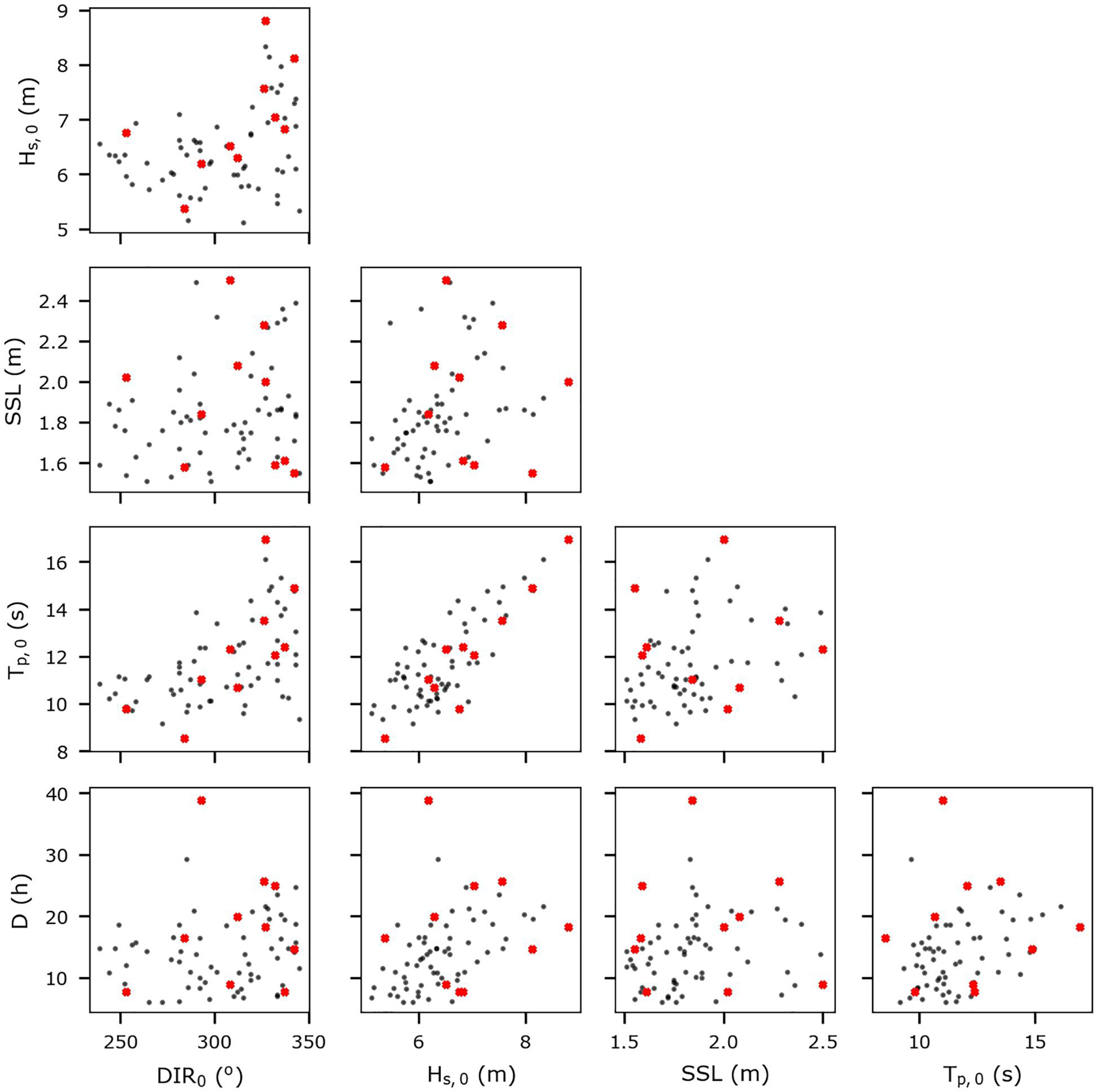
Figure 4. Scatter plots of offshore storm parameters pairs of the observed extreme events (black dots) extracted from the time-series at the four offshore locations. Red dots indicate the 10 most dissimilar events identified by the Maximum Dissimilarity Algorithm (MDA). Each scatter plot represents a pair of the offshore storm parameters: (1) Significant wave height (H_s,₀), (2) Peak wave period (T_p,₀), (3) Mean wave direction (Dir₀), (4) Storm surge level (SSL) and (5) event duration (D).

TABLE 1

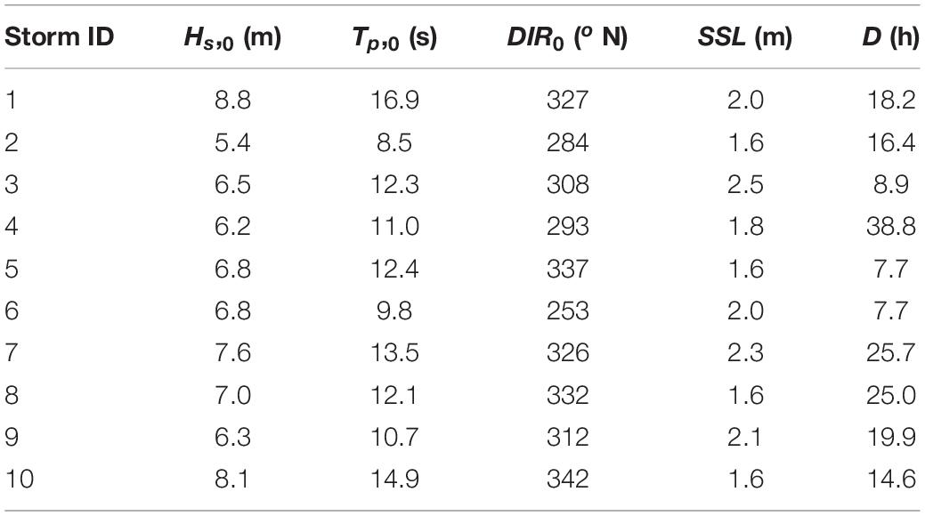
Table 1. Offshore storm parameters of the 10 most dissimilar extreme storm events identified by the Maximum Dissimilarity Algorithm (MDA).

Dune Erosion Modeling and Indicators

For the dune erosion computations we applied Xbeach which is an open-source, process-based model which simulates short wave energy and long wave transformation, wave-driven currents, sediment transport and corresponding morphological changes at sandy coasts (Roelvink et al., 2009). In the present study, XBeachX (v1.23) was used in a “surfbeat” mode, where the short-wave variations are resolved at the wave group scale. This mode has been extensively validated in dissipative beaches (such as the Dutch coast) where infragravity waves dominate the hydrodynamics and morphodynamics. A one-dimensional (1D) cross-shore model was created for each study transect, with the grid resolution varying across the profile, having finer resolution in the dune area. The topo-bathymetry was extracted from each individual JARKUS transect and was extended to a 30 m depth assuming a slope of 0.01, to make sure that the offshore boundary was deep enough so that the waves are in intermediate water (while the land boundary was defined by the most landward JARKUS profile point).

For each storm, the offshore parameters (Figure 4 and Table 1) were used to construct the XBeach boundary conditions of time-varying surface elevations and wave energy at the wave group scale. For the time evolution of H_s during each storm, a triangular approach was used (Supplementary Section 2), while for T_p it was assumed that the wave steepness (derived from the maximum H_s and T_p during the storm) stays constant throughout the event. DIR was assumed constant throughout the event. These wave time series were then used to construct JONSWAP spectra time series (gamma = 3.3 and wave directional spreading of 30°) that were imposed at the offshore boundary of the model (Figures 5A,B). For the water levels, a SSL curve was created by rescaling the normalized hydrograph extracted from the historic events (Supplementary Section 2), using the maximum SSL and D of the individual event. A tidal signal was used for each profile based on observed tidal records and the local MHW (see Supplementary Section 2). The superimposition of the SSL and tidal signals was imposed at the offshore boundary of each model (Figure 5C), while the bound long waves were calculated internally by XBeach (Van Dongeren et al., 2003; Roelvink et al., 2009). Each XBeach 1D model, was forced with the exact same offshore storm conditions for each representative storm (except the local tidal amplitude), while the local profile orientation was included in the model to account for differences in wave energy exposure.

FIGURE 5

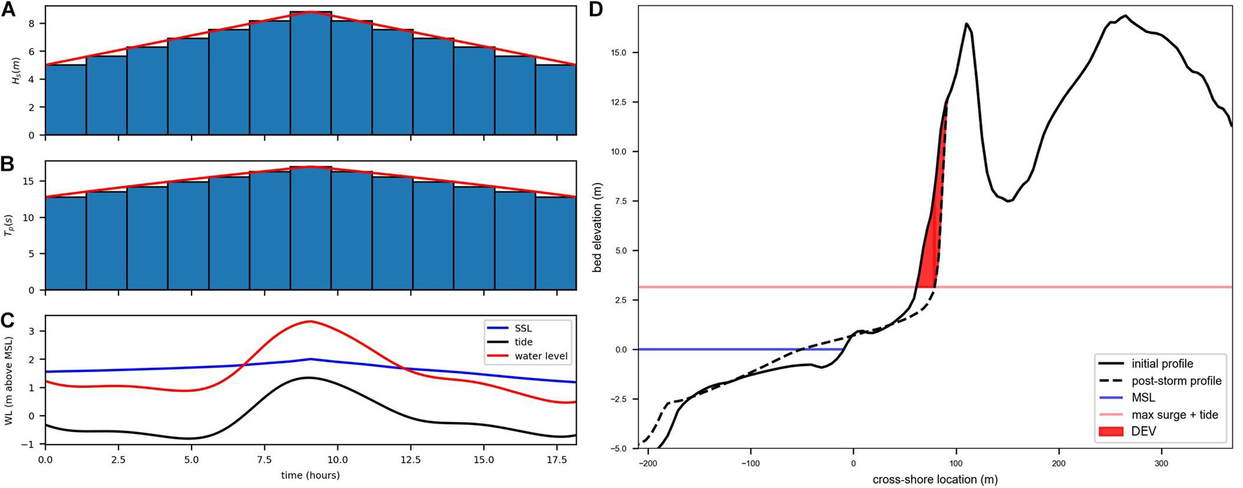
Figure 5. Example of XBeach offshore boundary conditions for Storm 1 (Figure 4 and Table 1), and of the dune impact for one test transect. (A) H_s time series (red line) and Hs for the JONSWAP spectrum (blue bars), (B) same as panel (A), but for T_p, (C) water level time series at offshore boundary. (D) Example of dune erosion volume (DEV) at transect 7002882 – see Figure 2.

Since the present study aims to propose a methodology for predicting dune morphodynamic response by identifying drivers for dune erosion and grouping similar coastal profiles, but not to directly produce a predictive tool, the “default values” of XBeach (Deltares, 2018) were applied without any further calibration. Considering that a large number of simulations needed to be run (1,430 profiles × 10 storms = 14,300 simulations), various model parameters (morphological acceleration factor (morfac) (Roelvink et al., 2009), maximum Courant-Friedrichs-Lewy number (CFL) and grid resolution) were tested to reduce the computational time without affecting the dune response significantly (relatively to the default parameters). The tests were performed for the five most dissimilar storms and for 10 profiles with diverse morphological characteristics, to ensure that the results captured a broad spectrum of profile geometries and boundary conditions. Based on the outcomes of these tests, a morfac of 5, a CFL of 0.9 and a grid resolution of 1 m in the dune area were selected.

Here, the dune erosion volume (DEV), defined as the volume of dune loss above the maximum surge and tide level during an event and landward of the pre-storm dune toe (Figure 5D), was chosen as the dune impact indicator (Giardino et al., 2014) and was calculated for all profiles and storms that were simulated.

The presence of linear correlations between the spatial variability of the computed DEVs for each storm (section “Representative Offshore Storms”) and each morphological (section “Morphological Parameters”) and hydrodynamic (section “Hydrodynamic Parameters”) parameter along the Dutch coast were explored by calculating Pearson correlations (r) (section “Dune Erosion Drivers”). This initial analysis provided an overview of the sensitivity of the dune impact (DEV) to profile characteristics (both morphological and hydrodynamic) and was used as a pre-filtering guide for the parameter combinations used in the clustering phase (section “Clustering Sensitivity Analysis”). Additionally, the DEV dataset acted as a benchmark for the cross-validation of the proposed prediction techniques (section “Prediction and Validation”).

Clustering of Coastal Profiles

In order to group similar coastal profiles and identify TCPs that are representative of each group, unsupervised multivariate clustering techniques (Hastie, 2017) were employed, using the morphodynamic, hydrodynamic or dune erosion parameters that were calculated per profile (see previous section). In the present study, different combinations of parameters and different clustering algorithms were tested (K-means, K-medoids, and Hierarchical clustering, see Supplementary Section 3). A clustering example with nine clusters (number of clusters chosen to enable easy visualization), using K-means on five morphological parameters (equally weighted in this example) is presented in Figure 6. In this example, profiles are grouped based on these specific characteristics (Foredune crest z, Max dune volume, Beach width, Beach volume, and Nearshore slope), with, for example, cluster 1 representing the most frequently encountered type of profiles with relatively minor beach size and mild nearshore slopes, cluster 7 representing profiles with large beach features but lower dune features, while cluster 8 profiles that have steep nearshore slopes.

FIGURE 6

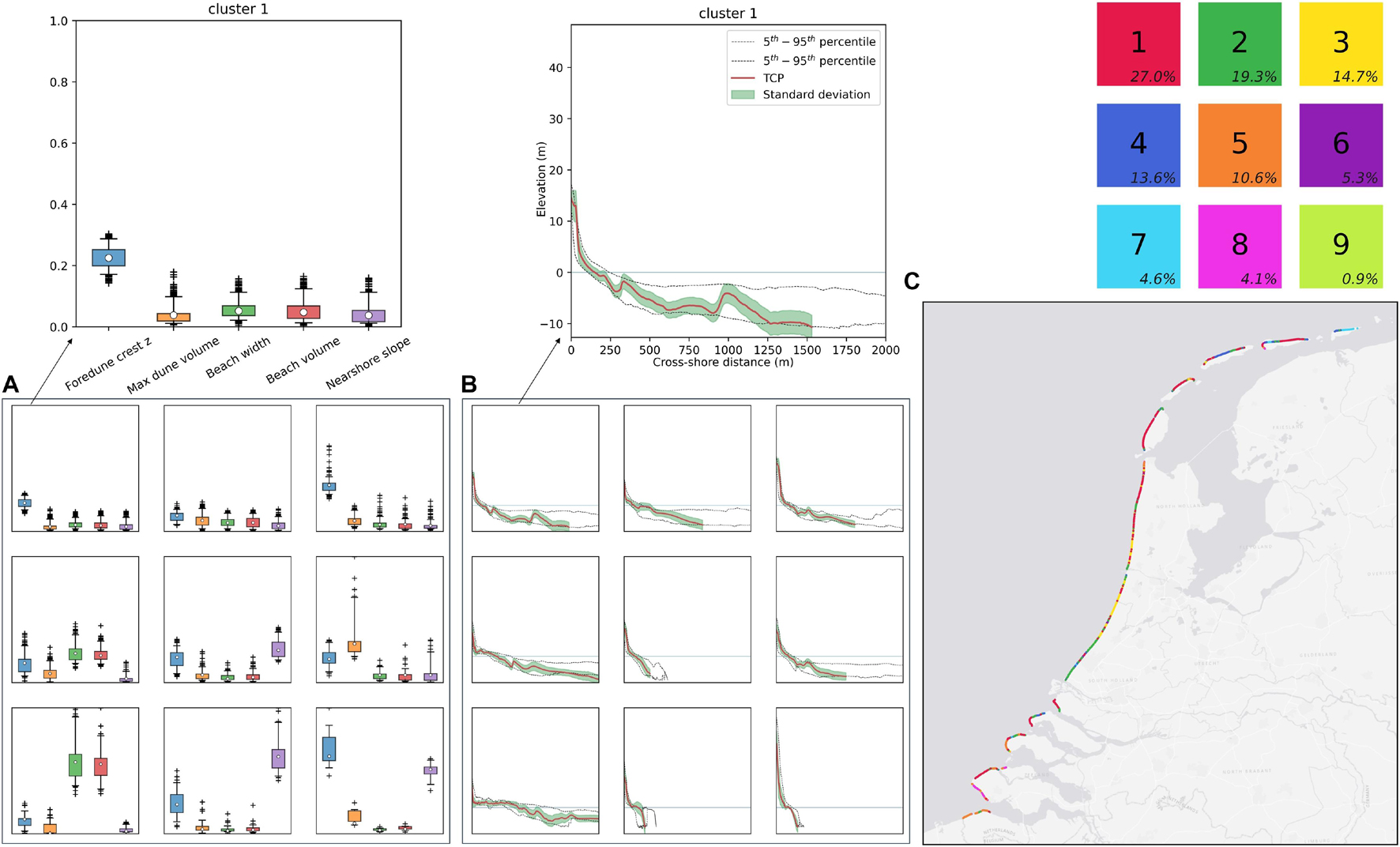
Figure 6. Example of clustering the 1430 JARKUS profiles with K-means into nine clusters (TCPs) using the foredune crest z, max dune volume, beach width, beach volume and nearshore slope as clustering parameters. (A) Boxplots of intra-cluster scaled parameters variability. Boxes define the 25–75% percentile, lines the 5–95% percentile and crosses outliers. Circles indicate the TCP of each cluster. (B) TCPs and intra-cluster elevation profile variability. Profiles are plotted from the foredune crest to the depth of closure. (C) Map of clustering of the Dutch profiles. The cluster number, frequency of appearance and color are shown in the grid at the top right, which is the same order as the grid at panels (A,B). Cluster numbers are ordered by frequency of appearance.

The clustering example presented in Figure 6 grouped the profiles based on a chosen set of morphological parameters only and used a rather low number of clusters to demonstrate the procedure. But, as mentioned in section “Hydrodynamic Parameters”, spatial variability in hydrodynamic parameters can affect dune response variability during extreme events as well. Therefore, different combinations of the morphological and hydrodynamic parameters and weighting factors were tested using the developed DEV benchmark dataset (section “Dune Erosion Modeling and Indicators”) to validate the representativeness of the selected TCPs with respect to dune response (section “Prediction and Validation”) and are presented in section “Clustering Sensitivity Analysis.” Then, using the simulated DEVs of these initial TCPs in a 2nd clustering step, the profiles were further reduced to a smaller number of final TCPs, using their dune response explicitly. This entire clustering approach defined herein as 2-step clustering (Figure 1) can be summarized as follows:

(1) A 1st clustering of profiles based on a combination of morphological and hydrodynamic parameters to obtain N number of initial TCPs (iTCPs). The number of iTCPs N should always be larger than the number of final TCPs M. Here, different values of N were tested, and a value of N = 300 iTCPs was chosen based on an elbow approach (Scott et al., 2020; see Supplementary Figure 4), ensuring a high inter-cluster similarity while having a small number of iTCPs.

(2) A 2nd clustering of the N = 300 iTCPS based on the same combination of their morphological and hydrodynamic parameters (50% weighting) as in the 1st clustering, but now adding the 10 individual DEV parameters simulated for each of the representative storms and each iTCP as extra clustering attributes (50% weighting), to get M number of TCPs. In this 2nd clustering, the morphological and hydrodynamic parameters are used again (with a 50% weighting in total), to preserve some profile descriptive information in the clustering process and avoid having profiles that might have completely different morphological characteristics but similar dune response, in the same cluster. Different numbers M of TCPs were considered (10, 50, 100, and 200) to test the influence of this number on the clustering performance.

Prediction and Validation

To make a DEV prediction for a new “unseen” profile, it must be matched to one or more of the previously derived TCPs by using a similarity indicator. Since, for this “unseen” profile, an XBeach simulation will not be available, the matching should be performed based only on morphological and hydrodynamic parameters (same used during the 1st clustering step). This means that the test profile will be first matched to the iTCPs and then the TCP assignments of the iTCPs will be followed to finally match the test profile with the TCPs. Two matching methods were compared following Scott et al. (2020). First, a direct matching approach was tested, which was simply done by matching the test profile with the most similar iTCP, defined by the smallest pairwise distance between the test profile and the iTCPs. The same distance metric as in the clustering was used to calculate the pairwise distances. Secondly, a probabilistic matching was tested, assigning matching probabilities to each iTCP according to the pairwise distances. The matching probabilities of a test profile to the iTCPs were calculated using the softmax function:

$$P\left(i\right)=\frac{{\text{e}}^{(-B\cdot x_i)}}{{\sum }_{j=1}^N{\text{e}}^{(-B\cdot x_j)}}(1)$$

Where P(i) is the probability of matching to iTCP i, x_i is the distance between the test profile and the iTCP i, x_j is the distance between the test profile and the iTCP j, B is the stiffness parameter and N is the number of iTCPs (Scott et al., 2020). Different values of B were tested, which essentially determined the variance of the probabilities, with larger B values resulting in larger probabilities for iTCPs associated with smaller distances. Ultimately the DEV prediction for the “unseen” profile is made either by (1) using the simulated DEV value of the single matched TCP in the case of direct matching or (2) the weighted average DEV value of the TCPs, using the previously described matching probabilities as weights. The two methods are compared for different number of clusters in section “Clustering Sensitivity Analysis” and (Figure 9B).

The predictive performance of the choice of different feature combinations, clustering algorithms, number of clusters, and matching methods used (referred from here onward as model) was assessed by a k-fold validation using the DEV data derived in section “Dune Erosion Modeling and Indicators” as benchmark. This cross-validation technique allows to assess the performance of the model to “unseen” data, therefore avoiding overfitting and artificial skill. The k-fold validation involved the following steps: (1) randomize the order of the 1,430 profiles in the dataset, (2) split the dataset in k subsets of equal size, (3) use 1st subset as test (“unseen”) data and the other k − 1 subsets as training data, (4) repeat 3rd step for each subset, (5) calculate average performance metrics of all k repetitions. After testing different k values, a k = 10 was used as that was the value for which the performance metrics stabilized and ensured that the model was well trained (∼1,300 profiles), while having a high enough number of profiles (∼150) left for validation. To make sure that the performance metrics were not biased to the randomization process (1st step), the procedure was repeated five times with different randomization seeds. For each performance metric the mean and standard deviation were calculated from the 50 (5 randomizations × 10 k-folds) results per metric.

The accuracy of the DEV predictions was mainly assessed with the skill score (Murphy, 1988):

$$Skill=1-\frac{RMS{E}^2}{{\mathrm{\sigma }}_{DE{V}_m}^2}(2)$$

$$RMSE=\sqrt{\frac{{\sum }_{i=1}^n{\left(DE{V}_p-DE{V}_m\right)}^2}{n}}(3)$$

where DEV_p and DEV_m are the predicted and simulated DEVs for all 10 storms of the test profiles, respectively, σ_DEVm is the standard deviation of the simulated DEVs and n is the number of predictions validated (i.e., 10 storms × 143 test profiles = 1,430). A skill value of 1 indicates a perfect prediction. The bias, RMSE and the modified index of Mielke (λ) (Duveiller et al., 2016; Santos et al., 2019) were also explored as performance metrics. The predictive capabilities of the model were assessed using the previously described performance metrics (Sections “Clustering Sensitivity Analysis” and “Applying the Typological Coastal Profiles”).

Results

Dune Erosion Drivers

The pronounced along-coast spatial variability of DEV during the different representative storms is related to the variability of the morphological pre-storm parameters, the orientation of the profiles and the local tidal amplitude (Figure 7). The highest median DEV is observed for storm 1 (∼ 63 m³/m) and the lowest for storm 2 (∼ 1.5 m³/m), which have the highest and lowest H_s,₀, respectively. Inter-storm variability in DEV statistics is associated with differences in the storm intensity, described by the different offshore storm ocean variables, and verified that the MDA performed a good job in picking diverse storms.

FIGURE 7

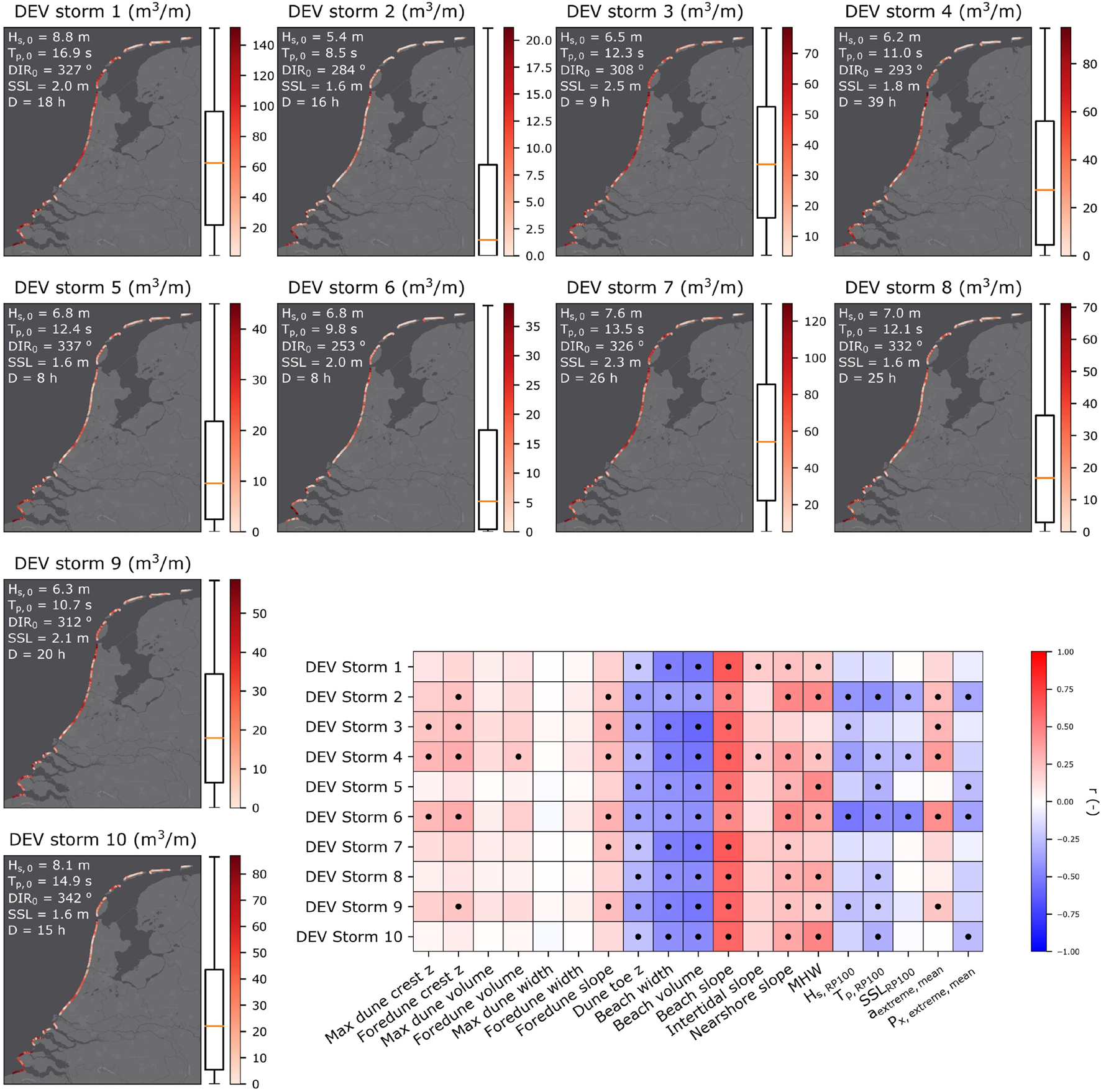
Figure 7. Dune erosion volume spatial variability and cross-correlation matrix for the 10 representative storms. The maps show the spatial distributions of DEV for each storm along with the offshore characteristics of each storm (top left of each map). The matrix at the bottom right shows the Pearson correlation coefficients between the DEV for each storm and various pre-storm morphological and hydrodynamic parameters at each profile. Dots indicate correlations with absolute values larger than 0.2 and significant at the 95% confidence level.

A first indication on the most important drivers of dune erosion variability along the Dutch coast was explored with Pearson correlations (r) between the DEV per storm and each morphological and hydrodynamic parameter studied herein (Figure 7). The calculated r were defined as significant when the absolute value was larger than 0.2 and it was statistically significant at the 95% level (Beuzen et al., 2019). The highest average (absolute) r values are found for the beach width (r = −0.46), beach volume (r = −0.49) and beach slope (r = 0.58), for which r is statistically significant for all storms. Next, it is the nearshore slope (r = 0.31) and MHW (r = 0.31), for which the relationship for storm 3 is not significant. This can be associated with storm 3 being the one with the highest SSL (2.5 m), which results in parameters such as the nearshore slope and MHW being less important, since the average depth increases. This pattern can be observed for all other storms, with lower SSL being associated with higher r values for the nearshore slope and MHW. The a_{extreme,  mean} parameter has an average r of 0.21 which is not significant for five storms associated with the largest DIR values (coming from the North).

In general, relationships can be identified between the strength of the correlation of a parameter with DEV and associated storm characteristics. For example, r values between DEV and dune parameters are generally higher for storms with smaller DIR values (incident from the West). Additionally, r values between DEV and pre-storm beach width and between DEV and pre-storm beach volume are higher for events with larger SSL values. These results suggest that the offshore storm characteristics (e.g., storm SSL) can affect how strongly the local coastal characteristics can drive dune erosion variability (Supplementary Figure 5). The other characteristic local hydrodynamic parameters (H_s,_RP100, T_p,_RP100, SSL_RP100, and P_x,_extreme,_mean) had average r values between −0.13 and −0.27. The negative correlation can relate to feedback mechanisms (e.g., coasts exposed to more severe offshore characteristics might have larger fronting beaches and/or milder nearshore slopes) and the fact the same offshore forcing was used for all profiles (i.e., profiles in Delta coast are exposed to less intense offshore conditions but when forced with a severe offshore storm they are prone to high DEV).

Clustering Sensitivity Analysis

A second analysis of the importance of parameters was performed on the basis of the actual DEV predictive skill when using 50 iTCPs produced with K-means and a direct matching method under a 10-fold cross-validation (Sections “Clustering of Coastal Profiles” and “Prediction and Validation”). For this analysis, only the 1st clustering step was performed, as the target was to optimize the morphological and hydrodynamic parameters combination. The choice of K-means and 50 iTCPs was based on minimizing the computational time, since a high number of combinations needed to be tested. All the parameters previously considered (Figure 7) were used, except the foredune and max dune widths which showed low correlation with DEV and were strongly correlated with other dune parameters, such as the dune volume (not shown here). All the potential combinations of the remaining 17 morphological and hydrodynamic parameters were tested (∼130,000 combinations), assuming the same weight for all respective parameters and the mean skill scores per combination were calculated. The frequency of appearance of each parameter in the top 1% performing combinations (Figure 8) and not the single best one was investigated, to avoid overfitting. The frequency of the appearance of the parameters in the top combinations indicated that their inclusion in the combinations provided valuable (regarding DEV prediction) information and showed a similar picture as in the correlation analysis (Figure 7). Differences mainly concerned the dune parameters and some of the wave parameters, as for example here the dune parameter with the highest frequency was the max dune volume which had a low average correlation. Additionally, the dune toe z, which had a significant correlation in the correlation analysis appeared only ∼25% of the time in the top combinations. These results suggest that when parameters are considered in combination, other interdependencies between them can be of importance. Using these results, the important parameters were chosen as the ones that had a frequency of more than 33% (e.g., appear at least 1 out of 3 times). A sensitivity analysis on the choice of this threshold showed small differences in the results, since the selected parameters are then weighted according to their contribution. Ultimately, the parameters that were selected for further analysis were: (a) from the morphological parameters: the max dune volume, beach width, beach volume, beach slope and nearshore slope; (b) from the hydrodynamic parameters: the MHW, T_p,_RP100, SSL_RP100, a_extreme,_mean, and P_{x,extreme, mean}.

FIGURE 8

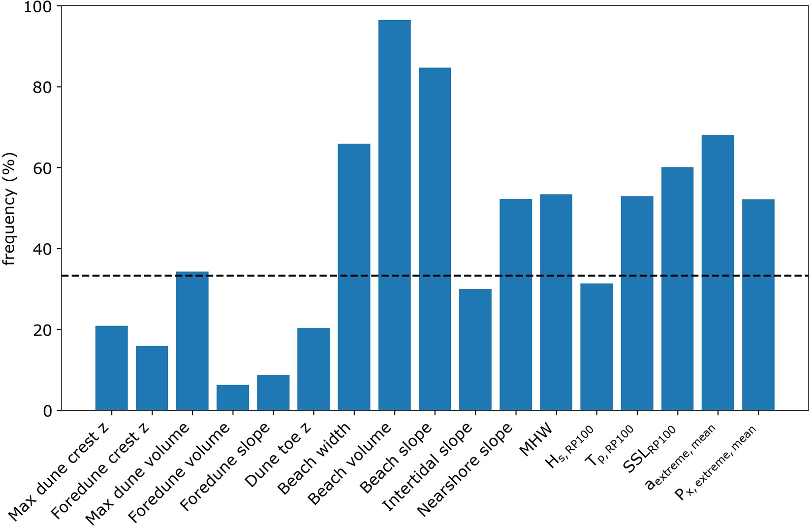
Figure 8. Frequency of occurrence of each potential parameter in the best performing combinations. Clustering was performed using a K-means algorithm and 50 clusters. The top performing combinations are the top 1% of the ∼130,000 possible combinations, defined on the basis of their skill score metric with a 10-fold validation. The dashed horizontal line indicated the 33% frequency.

In the previous tests where all the combinations of parameters were considered for the clustering procedure, all parameters had the same weight in the clustering algorithm. However, as it has been previously shown, some of the parameters can be more important in driving dune erosion variability during storms. To this end, an exhaustive/grid search approach was followed to find the optimum weights of each parameter for the clustering, by testing different weight combinations. The average weights (rounded at the 0.05 precision level) of the top 1% performing (on the basis of prediction skill) weights combinations were calculated and used as the final weighting in the clustering analysis (Table 2).

TABLE 2

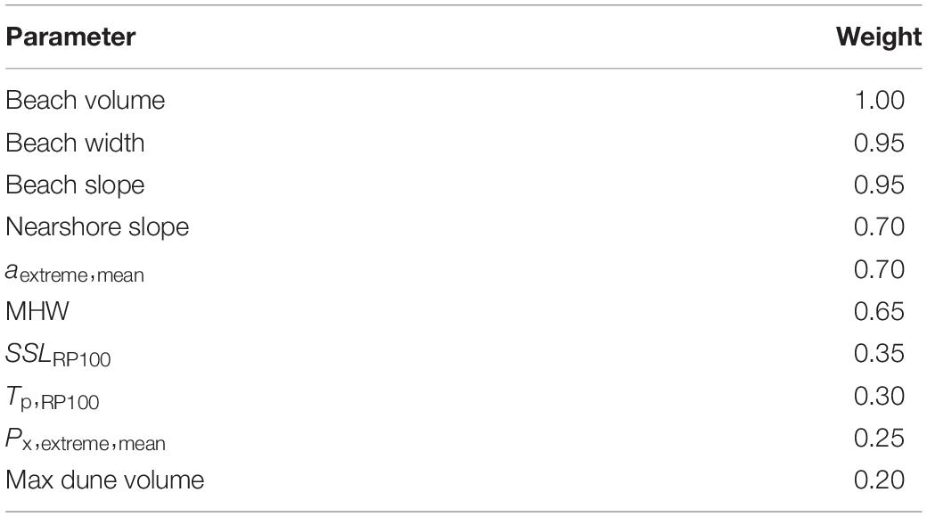
Table 2. Parameters weighting used in the clustering algorithms.

The proposed clustering algorithms (section “Clustering of Coastal Profiles”) were tested for different number of clusters (i.e., number M of TCPs) with a direct matching method and showed similar skill in predicting DEV (Figure 9A). It should be noted, that having similar skill does not mean that the same TCPs were chosen, but rather that similar predictive skills were obtained with the respective TCPs. To this end, the K-means clustering algorithm was used for the rest of the analysis as it was the fastest one between the three.

FIGURE 9

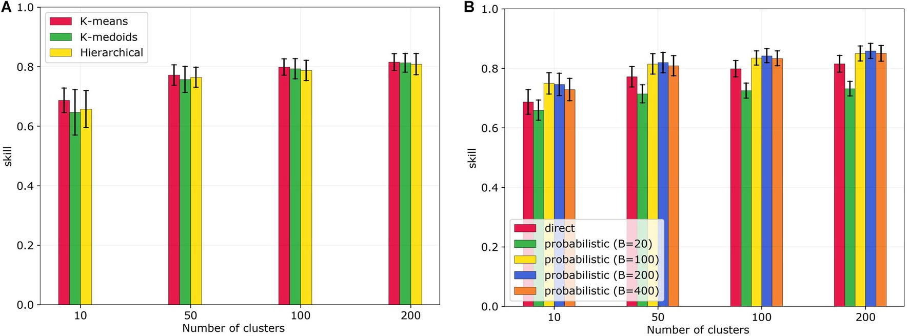
Figure 9. Sensitivity analysis for clustering algorithms and matching methods. (A) Prediction skill for different clustering techniques and number of clusters, using the direct matching method. (B) Prediction skill for different matching methods (direct and probabilistic with different B values) and number of clusters, using K-means clustering. Bars indicate the mean values and lines the standard deviation of the 10-fold cross-validation.

The different matching methods of the prediction model (section “Prediction and Validation”) were compared as well using K-means clustering and different number of TCPs (Figure 9B). For the probabilistic matching, different values of the stiffness parameter B were tested. The probabilistic matching mostly outperformed the direct matching method, except for small values B (i.e., less constrained weights). For the rest of the study, a probabilistic matching was used, with a B value of 200, since it performed best for the range of 100–200 clusters, which gives an acceptable input reduction and prediction skill combination.

Applying the Typological Coastal Profiles

Using the 2-step clustering approach with the aforementioned parameters combination and weighting, a K-means clustering algorithm and a probabilistic matching (stiffness parameter B = 200), the prediction capabilities were further investigated. Looking into the predicted DEV values versus the XBeach simulated DEVs (for all 10 storms) for one of the 10-fold cross-validations (143 test profiles), it can be observed, that as the number of clusters (TCPs) increases, the deviation from the 1:1 line (perfect prediction) decreases (Figure 10). These improved prediction capabilities are demonstrated by the performance metrics calculated (skill, λ, RMSE, and bias), which all attain improved values as the number of cluster increases (Figure 10). For M = 200 TCPs (i.e., highest number of clusters tested here), the skill score reaches a value of 0.86 with a RMSE of 13 m³/m. As described in section “Prediction and Validation,” the error metrics are presented for all 10 storms, but they can be calculated for the individual storms as well (Supplementary Figure 6). These were lower than the skill calculated using all the storms for all the number of clusters tested here, with an average skill of ∼0.6 for 10 clusters and ∼0.75 for 200 clusters.

FIGURE 10

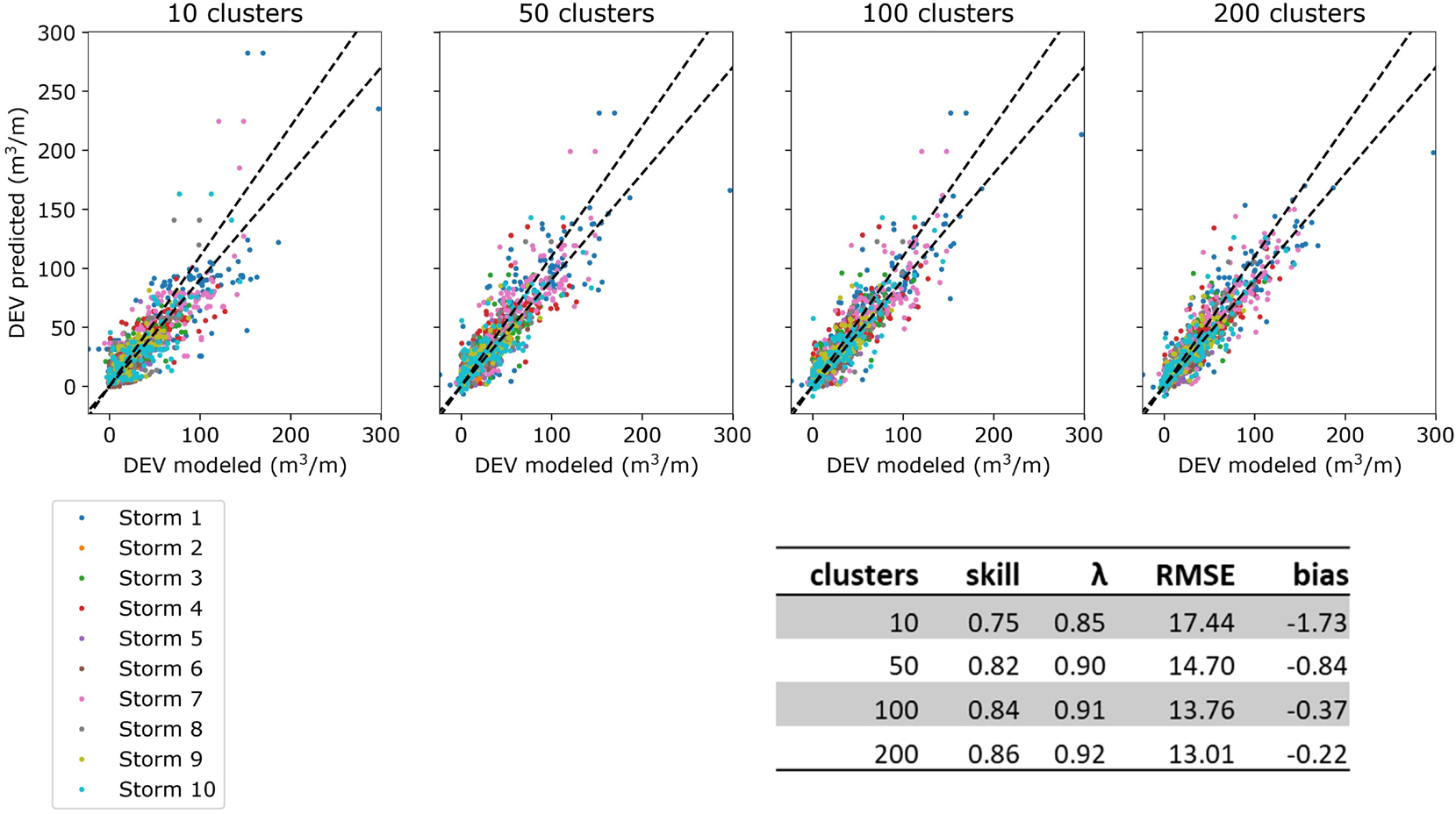
Figure 10. Scatter plots of simulated DEV with Xbeach vs. the predicted DEV for the 143 test profiles (10% of total profiles) and 10 storms, using a 2-step clustering with K-means (with 300 iTCPs) and a probabilistic matching (B = 200) for four different number of clusters (TCPs). The graphs indicate an example for one of the 10-fold cross-validations and points are colored for different storms. Dashed lines indicate a 10% deviation. At the bottom, the table shows the different mean error metrics of the 10-fold validation for each number of clusters (TCPs) used.

Since increasing the number of clusters always improves the error statistics (Figure 10), there is no optimum choice for the number of clusters/TCPs. However, a higher number of TCPs means a lower input reduction. Here, we used M = 100, since it provided a good input reduction with good prediction skill, reducing the JARKUS profiles (1,430) to 100 TCPs (Figure 11 and Supplementary Figure 7). It can be observed that ∼50% of all the profiles is already represented with 12 TCPs, while ∼90% can be represented by 47 TCPs (Figure 11A). The location of the TCPs shows that 18 of the 100 TCPs are on the Holland coast, 31 are on the Wadden coast and 51 on the Delta coast (Figure 11B). This indicates that the profiles on the Holland Coast are more coherent, while the profiles on the Delta coast are more diverse. The percentage of the TCPs per area relative to the total number of profiles per area were 13, 3, and 6% for the Delta, Holland and Wadden coasts, respectively. The representation of the TCPs for each area changes for the different number of TCPs tested here (Supplementary Figures 8, 9).

FIGURE 11

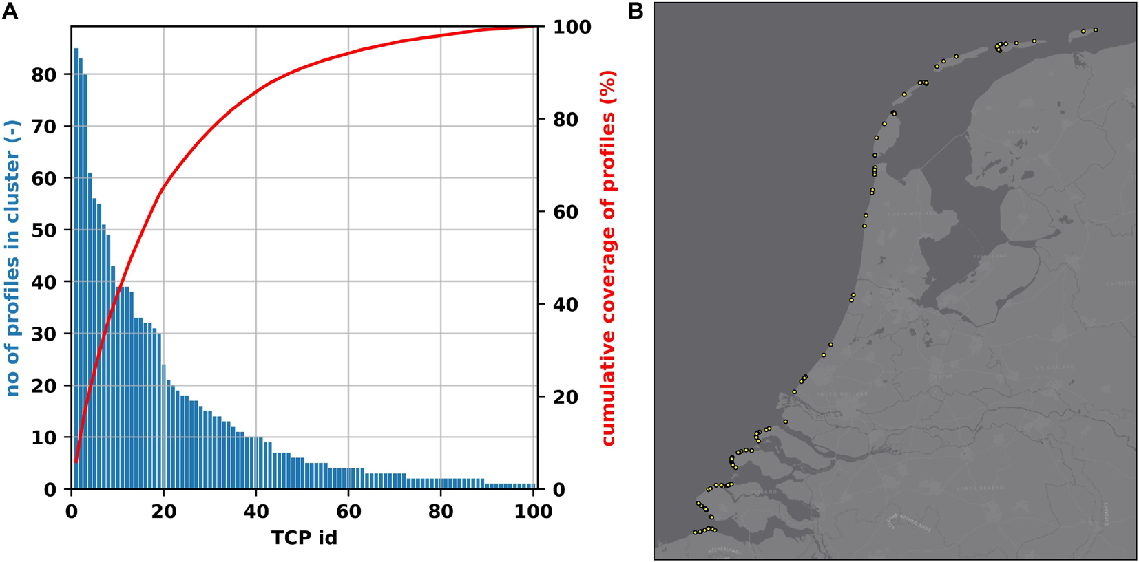
Figure 11. Typological coastal profiles (TCPs) for a 2-step clustering with K-means and 100 clusters. (A) Profile coverage of each TCP with bars and left axis showing the number of profiles per TCP and red line and right axis showing the cumulative coverage (%) of the profiles. The first 12 TCPs already describe ∼50% of all the profiles, while the first 47 TCPs describe ∼90% of all the profiles. (B) Map of the location of each of the 100 TCPs.

Discussion

Insights

The present study aimed at exploring the use of clustering approaches to reduce a large dataset of elevation transects to a fewer number of representative transects in order to facilitate the more efficient assessment of dune erosion due to extreme storms using the Dutch coast as a case study. We found that 1,430 profiles could be reduced to 100 representative ones, which would imply a large computational cost savings. The results furthermore highlight the importance of the shape of the beach fronting the dune systems in driving dune erosion variability during extreme coastal storms, with pre-storm beach width, volume and slope being in the most important parameters with respect to both the correlation analysis (section “Dune Erosion Drivers”) and the clustering analysis (section “Clustering Sensitivity Analysis”). These results agree with previous observations from measured changes in dune volume along the United States West Coast (Cohn et al., 2019) and at the southeast Australian coast (Beuzen et al., 2019). Additionally, the inclusion of the observed mean angle of incidence during extreme events (a_{extreme,  mean}), which represents both the local wave climate and profile orientation, improved the DEV prediction skill of the clustering approach, due to the variability in profile orientation along the Dutch coastline studied herein. The local nearshore slope, driving the wave dissipation and the MHW contributing to the total water level were found to be important driving parameters as well. Moreover, it was found that the importance of the morphological drivers can be dependent on the extreme storm characteristics with, for example, higher SSL making the beach characteristics stronger drivers of DEV spatial variability. The pre-storm dune parameters did not play an important role in driving DEV for the case of the Dutch coast, which is potentially related to the fact that dunes in the Netherlands are quite large with high features, seldomly being overwashed even during extreme events. This agrees with previous observations from Beuzen et al. (2019), where the dune characteristics were not found to be important for DEV predictions.

While the correlation analysis of the linear dependencies between DEV and the profile parameters provided a useful basis for exploring the importance of these characteristics for dune erosion, the clustering analysis provided new insights, taking into account the interdependencies between some of the parameters, since they were used in combination. Parameterizing each profile and then using these parameters in a clustering procedure, led to a descriptive grouping of the profiles, where profiles with similar characteristics were grouped together (e.g., profiles with high foredune and narrow beaches formed one cluster). But when accounting for the individual importance of each parameter in driving dune erosion the clustering techniques showed significant predictive skill in estimating DEV at “unseen” profiles, which highlights the potential use of this subset in a large-scale predictive tool.

As described in section “Clustering of Coastal Profiles,” a two-step clustering approach was followed herein, which uses simulated DEV for 10 representative storms in a 2nd clustering step, that re-clusters the initial typological profiles (iTCPs) in the final TCPs. However, since the correlation and feature combination analysis (sections “Dune Erosion Drivers” and “Clustering Sensitivity Analysis”) already ensured that the combination of morphological and hydrodynamic parameters used in the clustering phases consider the erosion driving processes, the 2nd clustering step could be potentially skipped and the iTCPs could directly act as TCPs (i.e., 1-step clustering). A comparison of the skill metrics of the 1-step clustering versus 2-step clustering with different number of TCPs is shown in Table 3. As expected, for all cases an increase in the number of clusters (TCPs) results in an improvement of skill. Additionally, the skill improvement with increasing number of clusters (TCPs) is more evident for the case of the 1-step clustering. Already, with 10 TCPs the skill score of the 2-step clustering is 0.3 larger than that for the 1-step clustering, while only for 200 TCPs the error statistics attain similar values for the two methods. This highlights the added value of using the simulated DEV in the clustering procedure.

TABLE 3

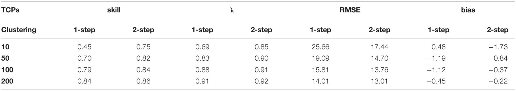
Table 3. Error statistics for 2-step and 1-step clustering using different number of typological coastal profiles (TCPs).

Generally, with the 2-step clustering a better prediction skill is attained for the same number of clusters (with increasing gain for lower number of clusters), relatively to the 1-step clustering. However, there is a compromise in the input data demands, since for the 2-step clustering, DEV observations or simulations need to be at hand for a number of profiles (equal to the chosen number of iTCPs in the 1st step clustering), while for the 1-step clustering only the morphological and hydrodynamic variables (which are easier to calculate) are needed. Ultimately, choosing between the two clustering techniques depends on the amount of input reduction needed for the specific application of the calculated TCPs, since for a small number of TCPs (i.e., high input reduction), a 2-step clustering would be necessary, to get a good prediction skill. The extra morphodynamic simulations that would be then needed for the 2nd clustering, could worth the extra workload, if they significantly decrease the computational burden for the final application. Additionally, this choice can relate to the needed accuracy of the final application, which could enable the use of 1-step clustering even for a smaller number of TCPs for more explorative and qualitative studies.

Limitations

In order to transform the offshore wave time-series to nearshore ones, a simple linear wave transformation and Snell’s law were applied with the implied assumption of an alongshore uniform bathymetry. Since this transformation was performed only to derive a proxy of the extreme nearshore hydrodynamic parameters characterizing each profile (section “Hydrodynamic Parameters”), a more elaborate approach based on wave modeling (Gouldby et al., 2014) was deemed out of the scope of this explorative study. Furthermore, this more generally applicable methodology has larger potential for upscaling this kind of studies globally, using offshore wave reanalysis or future scenario simulations (Vousdoukas et al., 2018). Additionally, in order to be able to apply our techniques for non-observed storms, we used schematized time-series for the wave conditions and SSL, when forcing XBeach, instead of actual observed time series. However, it should be noted that the use of a triangular distribution has been shown to introduce extra uncertainties in estimated DEVs (Duo et al., 2020), which are dependent on the initial profiles, thus affecting the computed DEV. Our methodology can be improved by considering synthetic hydrographs (Rizwan et al., 2019), however, such an effort would involve substantial computational effort. Given the fact that the schematized hydrographs showed a good agreement on the basis of a number of bulk parameters known to affect dune erosion (see Supplementary Section 2), here we decided to follow this simpler methodology.

Since pre and post-storm surveys were not available at this scale (as only annual observations are in the data set), dune impacts were simulated using a well-established dune erosion model and a set of representative storms at the Dutch coast. Xbeach has been shown to perform well in capturing the physical processes at dissipative sandy beach and dune coasts during storms in numerous previous studies (Lindemer et al., 2010; McCall et al., 2010; Vousdoukas et al., 2011; de Winter et al., 2015; Mickey et al., 2018; Passeri et al., 2018); and since the aim of the study was not to develop a predictive tool but rather to develop a methodology for making more efficient predictions of dune morphodynamics, the default settings of the model were used. Certainly, this is expected to influence the magnitude of simulated DEV along the Dutch coast. A consistent sensitivity analysis to test the influence of using the default parameters was not performed in this study but it is expected that while the magnitude of DEV could be affected, the general spatial variability and trends observed herein (which are more critical for the purposes of the study) will not be strongly influenced. Furthermore, the results presented herein are representative of dissipative coasts, where infragravity waves are driving coastal hydrodynamic and erosion. Possibly other parameters and other modeling tools (McCall et al., 2014) would be needed to apply the presented techniques at steeper coasts.

Sediment grain size variability can influence variabilities in dune response, an effect that was not explicitly considered in the present study. While this could be an important aspect in a global study including various study sites with a large range of grain sizes, we expect a small effect at the Dutch coast where the variability of D50 at the foredune along the coast is not that pronounced (Supplementary Figure 10) having a mean value of ∼210 μm and a standard deviation of ∼30 μm. The mean value along the Dutch coast is close to the default D50 value used in the Xbeach simulations herein, which is 200 μm. Considering the actual variability of D50 is expected to have minor effects in the simulated DEVs, since XBeach has little sensitivity to the D50 parameter (Ellen Quataert, Deltares, personal communication). Furthermore, the grain size variability is implicitly considered to some extent, since it is expected to be physically correlated with some of the other parameters used in the clustering procedure (e.g., beach slope).

With respect to the clustering of the profiles and defining the TCPs, various sensitivities were tested in the study herein, mainly focusing on (1) the parameters used, (2) their weights, (3) the clustering algorithm and (4) the matching technique. With respect to the parameters used, the extraction of parameters per profile was based on data availability and previous studies that explored their importance in driving dune erosion (Beuzen et al., 2019; Cohn et al., 2019; Santos et al., 2019). Undoubtedly, there are parameters that were not studied here and could be of importance for simulating the dune erosion more accurately and obtaining a better grouping of the profiles and thus more representative TCPs. These parameters could for example, be the local sand grain size (discussed previously) or the presence of vegetation on the dune (Charbonneau et al., 2017; Feagin et al., 2019). Three clustering algorithms were tested which fall in the categories of centroid-based clustering (K-means and K-medoids) and connectivity-based clustering (hierarchical). Other clustering techniques, based on other concepts are available as well, but were not tested here, due to the high number of profiles in the initial dataset, the high dimensionality (large number of parameters to be tested) and the computational constrains. For example, distribution-based algorithms like the Gaussian mixture models, might present some benefits for better clustering the coastal profiles, but are computationally expensive, restricting their application in the present study. Even though, comparing K-means, K-medoids and hierarchical clustering, resulted in quite similar prediction skill, the actual TCPs were different between the algorithms. This is expected to be of greater importance, when a small number of clusters (TCPs) is used, but as the intra-cluster variability decreases with an increasing number of clusters, the TCPs for a high number of clusters are expected to be similar between the algorithms.

On the Dutch coast, the dunes remain mostly in a swash or collision regime even during extreme events (flooding hazard scale by Sallenger, 2000) due to their considerable size and height. This means that while dune scarping can be expected during storms, overwash or inundation is not. Additionally, there is frequent maintenance of the Dutch dunes with sand nourishments. To this end, DEV was chosen as a descriptive indicator of dune erosion for the present study. Other indicators, such as foredune crest lowering, dune toe recession, beach width change and others, were tested but were disqualified due to either luck of variability or inconsistencies in the calculations. For example, due to the high dune features of the Dutch coast, foredune crest lowering was only seldomly observed in the modeled profiles. Additionally, in some other cases dune toe detection was not consistent in the pre-storm and post-storm profiles (i.e., erroneous detection of dune toe in post-storm profile) leading to inconsistencies in calculating the relative change, which could potentially introduce artificial inhomogeneities during the clustering phase. It would be expected tough, that for locations with barriers islands and lower dune features, other indicators like dune crest lowering or overwash volumes might be of more importance (Santos et al., 2019).

The presented methodology was built upon a specific dataset of coastal elevations and hydrodynamic conditions covering the Dutch coast and its specific range of potential values for each of the descriptive parameters used. Consequently, the derived TCPs have characteristic parameters that belong to that same range. Since the matching of an “unseen” test profile with one of the TCPs is performed on the basis of their similarity, there is no threshold that defines a minimum similarity when this matching is performed. This means that a profile with strongly different characteristics than any of the TCPs would still be matched to the TCP that is the most similar (on the basis of the distance metric used), but with a more uncertain DEV prediction. To that end, a threshold for the similarity could be applied, which when reached, the new profile should be considered as a new TCP itself and thus a set of new descriptive coastal change simulations would need to be performed. This threshold could be defined based on the maximum intra-cluster distances to the respective TCP of the already defined clusters. In the absence of such threshold, the decision of the number of TCPs can become more critical, to ensure that the test profiles are matched to similar TCPs with meaningful DEV prediction.

Implications

Large scale assessments and coastal screening studies are often based on tools or meta-models that enable efficient prediction of impact indicators (Viavattene et al., 2017; Athanasiou et al., 2020; Sanuy and Jiménez, 2021). The proposed input reduction methodology can be incorporated in such tools to reduce computational costs and enable the inclusion of more forcing scenarios. This could be useful for example in (1) early warning systems, when computational time is critical or (2) probabilistic long-term coastal vulnerability probabilistic assessments, when a high number of simulations is required. Large scale probabilistic estimation of impact indicators can reveal spatial variabilities in erosion hazard and identify hotspots where more elaborate modeling (e.g., 2DH Xbeach) could be applied. The methodology can also be useful in case of changes in the hydrodynamic forcing (e.g., as a result of climate change) or morphological parameters (e.g., as a result of man-made interventions such as a nourishment), since the results can be directly updated on the basis of the new similarities of the pre-defined TCPs, instead of re-running all the simulations.

Additionally, the input dataset could be extended with more elevation profile datasets (Athanasiou et al., 2019) and storm conditions to capture a bigger range of coastal settings. Applying the presented clustering methodology to this extended dataset will produce more diverse TCPs, which capture a broader spectrum of coastal typologies. Since this extended set of TCPs would represent a higher range of coastal morphologies and/or local hydrodynamics, they could potentially be used to get a 1st order estimate of dune erosion hazard to extremes storms at data poor locations. For example, less accurate data (e.g., satellite derived DEMs) could be used to get information on the beach and nearshore characteristics for this kind of areas.

More specifically, the derived TCPs at the Dutch coast could be used in a Bayesian Network in combination with a high number of potential storm conditions and calibrated Xbeach 1D models, to: (1) assess the influence of different scenarios or/and climate change, (2) identify critical areas with respect to dune erosion along the Dutch coast and (3) provide a first qualitive assessment of sand nourishment volumes needed after a storm. For the case of the Dutch coast, a good prediction skill (0.84) of DEV was attained with at least 100 TCPs which represents a 93% input reduction from the initial 1,430 JARKUS profiles.

Conclusion

Clustering algorithms were employed in order to obtain a representative subset of sandy beach and dune profiles (called typological coastal profiles or TCPs) that can be used to describe the dune response to extreme events for a large domain (Dutch coast) at a much-reduced computational cost relative to a conventional brute force approach where individual profiles are assessed. These TCPs were chosen on the basis of various local morphological and hydrodynamic characteristics that have been shown to drive dune response during extreme events, while simulated DEVs under representative storms were accounted as well (i.e., 2-step clustering). Dune fronting pre-storm beach geometries, nearshore slopes, local tidal amplitude, and profile orientations were found to be the most important drivers of simulated DEV variability.

Using these insights, different clustering methodologies were tested, and their performance was explored through a cross-validation technique. Using 100 TCPs (a 93% input reduction relative to the initial 1,430 profiles) resulted in a good prediction skill (0.84) for DEV with an average RMSE of 13.8 m³/m. For the case of the Dutch coast, 47 of these TCPs already represent ∼90% of the total available profiles, with large stretches of the Wadden and Holland coasts being adequately represented by a small number of TCPs relatively to the Delta coast. An approach where simulations of DEV are not necessary, by using only the pre-storm morphological and hydrodynamic parameters for the clustering procedure (1-step clustering) was assessed as well. This method produced a skill score of 0.83 only when a higher number of 200 TCPs was used.

Ultimately, the final application of the TCPs, and thus the level of input (and thus computational cost) reduction or accuracy needed, would dictate the choice of the clustering approach and the number of TCPs used. Potential applications of the proposed methodology include incorporation in a Bayesian Network, enabling large scale probabilistic impact assessments. Additionally, expanding the input training data with globally available datasets of coastal elevations can contribute in upscaling the methodology for a first order assessments of dune erosion potential at data-poor coastal locations.

Data Availability Statement

The raw data supporting the conclusions of this article will be made available by the authors, without undue reservation.

Author Contributions

PA, AD, AG, MV, RR, and JA contributed to the design of the study. PA carried out the data processing, analysis, figure generation, and prepared the manuscript with contributions from all co-authors. All authors contributed to the article and approved the submitted version.

Funding

This work has received funding from the EU Horizon 2020 Program for Research and Innovation, under grant agreement no 776613 (EUCP: “European Climate Prediction system;” https://www.eucp-project.eu). AD was funded in part by the Deltares Strategic Research Programme “Natural Hazards”, while AG from the Research Programme “Seas and Coastal Zones”. RR is supported by the AXA Research fund and partly supported by the Deltares Research program “Seas and Coastal Zones”.

Conflict of Interest

The authors declare that the research was conducted in the absence of any commercial or financial relationships that could be construed as a potential conflict of interest.

Publisher’s Note

All claims expressed in this article are solely those of the authors and do not necessarily represent those of their affiliated organizations, or those of the publisher, the editors and the reviewers. Any product that may be evaluated in this article, or claim that may be made by its manufacturer, is not guaranteed or endorsed by the publisher.

Acknowledgments

The maps of the Figures were created with Python 3.7.3 (https://www.python.org) using the Geopandas (v0.6.2, https://geopandas.org/) and Matplotlib (v3.1.2, https://matplotlib.org/) libraries.

Supplementary Material

The Supplementary Material for this article can be found online at: https://www.frontiersin.org/articles/10.3389/fmars.2021.747754/full#supplementary-material

References

Almar, R., Ranasinghe, R., Bergsma, E. W. J., Diaz, H., Melet, A., Papa, F., et al. (2021). A global analysis of extreme coastal water levels with implications for potential coastal overtopping. Nat. Commun. 12:3775. doi: 10.1038/s41467-021-24008-9

PubMed Abstract | CrossRef Full Text | Google Scholar

Arens, S. M., and Wiersma, J. (1994). The Dutch foredunes: inventory and classification. J. Coast. Res. 10, 189–202.

Google Scholar

Athanasiou, P., de Boer, W., Yoo, J., Ranasinghe, R., and Reniers, A. (2018). Analysing decadal-scale crescentic bar dynamics using satellite imagery: a case study at Anmok beach, South Korea. Mar. Geol. 405, 1–11. doi: 10.1016/j.margeo.2018.07.013

CrossRef Full Text | Google Scholar

Athanasiou, P., van Dongeren, A., Giardino, A., Vousdoukas, M. I., Ranasinghe, R., and Kwadijk, J. (2020). Uncertainties in projections of sandy beach erosion due to sea level rise: an analysis at the European scale. Sci. Rep. 10:11895. doi: 10.1038/s41598-020-68576-0

PubMed Abstract | CrossRef Full Text | Google Scholar

Athanasiou, P., van Dongeren, A., Giardino, A., Vousdoukas, M., Gaytan-Aguilar, S., and Ranasinghe, R. (2019). Global distribution of nearshore slopes with implications for coastal retreat. Earth Syst. Sci. Data 11, 1515–1529. doi: 10.5194/essd-11-1515-2019

CrossRef Full Text | Google Scholar

Ballesteros, C., Jiménez, J. A., Valdemoro, H. I., and Bosom, E. (2018). Erosion consequences on beach functions along the Maresme coast (NW Mediterranean. Spain). Nat. Hazards 90, 173–195. doi: 10.1007/s11069-017-3038-5

CrossRef Full Text | Google Scholar

Beuzen, T., Harley, M. D., Splinter, K. D., and Turner, I. L. (2019). Controls of variability in berm and dune storm erosion. J. Geophys. Res. Earth Surf. 124, 2647–2665. doi: 10.1029/2019JF005184

CrossRef Full Text | Google Scholar

Beuzen, T., Splinter, K. D., Marshall, L. A., Turner, I. L., Harley, M. D., and Palmsten, M. L. (2018). Bayesian Networks in coastal engineering: distinguishing descriptive and predictive applications. Coast. Eng. 135, 16–30. doi: 10.1016/j.coastaleng.2018.01.005

CrossRef Full Text | Google Scholar

Beuzen, T., Splinter, K. D., Turner, I. L., Harley, M. D., and Marshall, L. (2017). “Predicting storm erosion on sandy coastlines using a Bayesian network,” in Proceedings of the 16th Australasian Port and Harbour Conference 2017, Cairns, Qld, 102–108.

Google Scholar

Camus, P., Mendez, F. J., Medina, R., and Cofiño, A. S. (2011). Analysis of clustering and selection algorithms for the study of multivariate wave climate. Coast. Eng. 58, 453–462. doi: 10.1016/j.coastaleng.2011.02.003

CrossRef Full Text | Google Scholar

Castelle, B., Marieu, V., Bujan, S., Splinter, K. D., Robinet, A., Sénéchal, N., et al. (2015). Impact of the winter 2013-2014 series of severe Western Europe storms on a double-barred sandy coast: beach and dune erosion and megacusp embayments. Geomorphology 238, 135–148. doi: 10.1016/j.geomorph.2015.03.006

CrossRef Full Text | Google Scholar

Charbonneau, B. R., Wootton, L. S., Wnek, J. P., Langley, J. A., and Posner, M. A. (2017). A species effect on storm erosion: invasive sedge stabilized dunes more than native grass during Hurricane Sandy. J. Appl. Ecol. 54, 1385–1394. doi: 10.1111/1365-2664.12846

CrossRef Full Text | Google Scholar

Chiri, H., Abascal, A. J., Castanedo, S., Antolínez, J. A. A., Liu, Y., Weisberg, R. H., et al. (2019). Statistical simulation of ocean current patterns using autoregressive logistic regression models: a case study in the Gulf of Mexico. Ocean Model. 136, 1–12. doi: 10.1016/j.ocemod.2019.02.010

CrossRef Full Text | Google Scholar

Cohn, N., Ruggiero, P., García-Medina, G., Anderson, D., Serafin, K. A., and Biel, R. (2019). Environmental and morphologic controls on wave-induced dune response. Geomorphology 329, 108–128. doi: 10.1016/j.geomorph.2018.12.023

CrossRef Full Text | Google Scholar

Davidson, S. G., Hesp, P. A., and da Silva, G. M. (2020). Controls on dune scarping. Prog. Phys. Geogr. 44, 923–947. doi: 10.1177/0309133320932880

CrossRef Full Text | Google Scholar

de Queiroz, B., Scheel, F., Caires, S., Walstra, D. J., Olij, D., Yoo, J., et al. (2019). Performance evaluation of wave input reduction techniques for modeling inter-annual sandbar dynamics. J. Mar. Sci. Eng. 7:148. doi: 10.3390/jmse7050148

CrossRef Full Text | Google Scholar

de Vries, S., Southgate, H. N., Kanning, W., and Ranasinghe, R. (2012). Dune behavior and aeolian transport on decadal timescales. Coast. Eng. 67, 41–53. doi: 10.1016/j.coastaleng.2012.04.002

CrossRef Full Text | Google Scholar

de Winter, R. C., Gongriep, F., and Ruessink, B. G. (2015). Observations and modeling of alongshore variability in dune erosion at Egmond aan Zee, the Netherlands. Coast. Eng. 99, 167–175. doi: 10.1016/j.coastaleng.2015.02.005

CrossRef Full Text | Google Scholar

Deltares (2018). XBeach Documentation: Release XBeach v1.23.5527 XBeachX FINAL. Available online at: https://oss.deltares.nl/web/xbeach/ (accessed October 20, 2020).

Google Scholar

Diamantidou, E., Santinelli, G., Giardino, A., Stronkhorst, J., and De Vries, S. (2020). An automatic procedure for dune foot position detection: application to the dutch coast. J. Coast. Res. 36, 668–675. doi: 10.2112/JCOASTRES-D-19-00056.1

CrossRef Full Text | Google Scholar

Duo, E., Sanuy, M., Jiménez, J. A., and Ciavola, P. (2020). How good are symmetric triangular synthetic storms to represent real events for coastal hazard modelling. Coast. Eng. 159:103728. doi: 10.1016/j.coastaleng.2020.103728

CrossRef Full Text | Google Scholar

Duveiller, G., Fasbender, D., and Meroni, M. (2016). Revisiting the concept of a symmetric index of agreement for continuous datasets. Sci. Rep. 6:19401. doi: 10.1038/srep19401

PubMed Abstract | CrossRef Full Text | Google Scholar

ESRI (2011). Light Gray Canvas. Basemap. Available online at: https://www.arcgis.com/home/item.html?id=8b3d38c0819547faa83f7b7aca80bd76 (accessed March 3, 2021).

Google Scholar

Feagin, R. A., Furman, M., Salgado, K., Martinez, M. L., Innocenti, R. A., Eubanks, K., et al. (2019). The role of beach and sand dune vegetation in mediating wave run up erosion. Estuar. Coast. Shelf Sci. 219, 97–106. doi: 10.1016/j.ecss.2019.01.018

CrossRef Full Text | Google Scholar

Giardino, A., Diamantidou, E., Pearson, S., Santinelli, G., and den Heijer, K. (2019). A regional application of bayesian modeling for coastal erosion and sand nourishment management. Water (Switzerland) 11:61. doi: 10.3390/w11010061

CrossRef Full Text | Google Scholar

Giardino, A., Santinelli, G., and Vuik, V. (2014). Coastal state indicators to assess the morphological development of the Holland coast due to natural and anthropogenic pressure factors. Ocean Coast. Manag. 87, 93–101. doi: 10.1016/j.ocecoaman.2013.09.015

CrossRef Full Text | Google Scholar

Gouldby, B., Méndez, F. J., Guanche, Y., Rueda, A., and Mínguez, R. (2014). A methodology for deriving extreme nearshore sea conditions for structural design and flood risk analysis. Coast. Eng. 88, 15–26. doi: 10.1016/j.coastaleng.2014.01.012

CrossRef Full Text | Google Scholar

Grzegorzewski, A. S., Cialone, M. A., and Wamsley, T. V. (2011). Interaction of barrier islands and storms: implications for flood risk reduction in Louisiana and Mississippi. J. Coast. Res. 2011, 156–164. doi: 10.2112/SI59-016.1

CrossRef Full Text | Google Scholar

Gutierrez, B. T., Plant, N. G., and Thieler, E. R. (2011). A Bayesian network to predict coastal vulnerability to sea level rise. J. Geophys. Res. Earth Surf. 116, 1–15. doi: 10.1029/2010JF001891

CrossRef Full Text | Google Scholar

Harley, M. D., Turner, I. L., Kinsela, M. A., Middleton, J. H., Mumford, P. J., Splinter, K. D., et al. (2017). Extreme coastal erosion enhanced by anomalous extratropical storm wave direction. Sci. Rep. 7:6033. doi: 10.1038/s41598-017-05792-1

PubMed Abstract | CrossRef Full Text | Google Scholar

Hastie, T. T. (2017). The Elements of Statistical Learning. New York, NY: Springer. doi: 10.1007/978-0-387-84858-7

CrossRef Full Text | Google Scholar

Houser, C., Hapke, C., and Hamilton, S. (2008). Controls on coastal dune morphology, shoreline erosion and barrier island response to extreme storms. Geomorphology 100, 223–240. doi: 10.1016/j.geomorph.2007.12.007

CrossRef Full Text | Google Scholar

Jongejan, R., Ranasinghe, R., Wainwright, D., Callaghan, D. P., and Reyns, J. (2016). Drawing the line on coastline recession risk. Ocean Coast. Manag. 122, 87–94. doi: 10.1016/j.ocecoaman.2016.01.006

CrossRef Full Text | Google Scholar

Keijsers, J. G. S., Giardino, A., Poortinga, A., Mulder, J. P. M., Riksen, M. J. P. M., and Santinelli, G. (2015). Adaptation strategies to maintain dunes as flexible coastal flood defense in The Netherlands. Mitig. Adapt. Strateg. Glob. Chang. 20, 913–928. doi: 10.1007/s11027-014-9579-y

CrossRef Full Text | Google Scholar

Li, F., van Gelder, P. H. A. J. M., Ranasinghe, R., Callaghan, D. P., and Jongejan, R. B. (2014). Probabilistic modelling of extreme storms along the Dutch coast. Coast. Eng. 86, 1–13. doi: 10.1016/j.coastaleng.2013.12.009

CrossRef Full Text | Google Scholar

Lindemer, C. A., Plant, N. G., Puleo, J. A., Thompson, D. M., and Wamsley, T. V. (2010). Numerical simulation of a low-lying barrier island’s morphological response to Hurricane Katrina. Coast. Eng. 57, 985–995. doi: 10.1016/j.coastaleng.2010.06.004

CrossRef Full Text | Google Scholar

Masselink, G., Scott, T., Poate, T., Russell, P., Davidson, M., and Conley, D. (2016). The extreme 2013/2014 winter storms: hydrodynamic forcing and coastal response along the southwest coast of England. Earth Surf. Process. Landforms 41, 378–391. doi: 10.1002/esp.3836

CrossRef Full Text | Google Scholar

McCall, R. T., Masselink, G., Poate, T. G., Roelvink, J. A., Almeida, L. P., Davidson, M., et al. (2014). Modelling storm hydrodynamics on gravel beaches with XBeach-G. Coast. Eng. 91, 231–250. doi: 10.1016/j.coastaleng.2014.06.007

CrossRef Full Text | Google Scholar

McCall, R. T., Van Thiel de Vries, J. S. M., Plant, N. G., Van Dongeren, A. R., Roelvink, J. A., Thompson, D. M., et al. (2010). Two-dimensional time dependent hurricane overwash and erosion modeling at Santa Rosa Island. Coast. Eng. 57, 668–683. doi: 10.1016/j.coastaleng.2010.02.006

CrossRef Full Text | Google Scholar

Mehvar, S., Filatova, T., Dastgheib, A., de Ruyter van Steveninck, E., and Ranasinghe, R. (2018). Quantifying economic value of coastal ecosystem services: a review. J. Mar. Sci. Eng. 6, 5. doi: 10.3390/jmse6010005

CrossRef Full Text | Google Scholar

Mickey, R., Long, J., Dalyander, P. S., Plant, N., and Thompson, D. (2018). A framework for modeling scenario-based barrier island storm impacts. Coast. Eng. 138, 98–112. doi: 10.1016/j.coastaleng.2018.04.012

CrossRef Full Text | Google Scholar

Monioudi, I. N., Velegrakis, A. F., Chatzipavlis, A. E., Rigos, A., Karambas, T., Vousdoukas, M. I., et al. (2017). Assessment of island beach erosion due to sea level rise: the case of the Aegean archipelago (Eastern Mediterranean). Nat. Hazards Earth Syst. Sci. 17, 449–466. doi: 10.5194/nhess-17-449-2017

CrossRef Full Text | Google Scholar

Murphy, A. H. (1988). Skill scores based on the mean square error and their relationships to the correlation coefficient. Mon. Weather Rev. 116, 2417–2424. doi: 10.1175/1520-04931988116<2417:SSBOTM<2.0.CO;2

CrossRef Full Text | Google Scholar

Paprotny, D., Terefenko, P., Giza, A., Czapliñski, P., and Vousdoukas, M. I. (2021). Future losses of ecosystem services due to coastal erosion in Europe. Sci. Total Environ. 760:144310. doi: 10.1016/j.scitotenv.2020.144310

PubMed Abstract | CrossRef Full Text | Google Scholar

Passeri, D. L., Long, J. W., Plant, N. G., Bilskie, M. V., and Hagen, S. C. (2018). The influence of bed friction variability due to land cover on storm-driven barrier island morphodynamics. Coast. Eng. 132, 82–94. doi: 10.1016/j.coastaleng.2017.11.005

CrossRef Full Text | Google Scholar

Pawlowicz, R., Beardsley, B., and Lentz, S. (2002). Classical tidal harmonic analysis including error estimates in MATLAB using TDE. Comput. Geosci. 28, 929–937. doi: 10.1016/S0098-3004(02)00013-4

CrossRef Full Text | Google Scholar

Pearson, S. G., Storlazzi, C. D., van Dongeren, A. R., Tissier, M. F. S., and Reniers, A. J. H. M. (2017). A Bayesian-Based system to assess wave-driven flooding hazards on coral reef-lined coasts. J. Geophys. Res. Ocean 122, 10099–10117. doi: 10.1002/2017JC013204

CrossRef Full Text | Google Scholar

Poelhekke, L., Jäger, W. S., van Dongeren, A., Plomaritis, T. A., McCall, R., and Ferreira, Ó (2016). Predicting coastal hazards for sandy coasts with a Bayesian Network. Coast. Eng. 118, 21–34. doi: 10.1016/j.coastaleng.2016.08.011

CrossRef Full Text | Google Scholar

Ranasinghe, R., Callaghan, D., and Stive, M. J. F. (2012). Estimating coastal recession due to sea level rise: beyond the bruun rule. Clim. Change 110, 561–574. doi: 10.1007/s10584-011-0107-8

CrossRef Full Text | Google Scholar

Rijkswaterstaat (2018). Jarkus Cross-Shore Profile Measurements Database. Available online at: https://publicwiki.deltares.nl/display/OET/Dataset+documentation+JarKus (accessed February 10, 2020).

Google Scholar

Rizwan, M., Guo, S., Yin, J., and Xiong, F. (2019). Deriving design flood hydrographs based on copula function: a case study in Pakistan. Water 11:1531. doi: 10.3390/w11081531

CrossRef Full Text | Google Scholar

Roelvink, D., Reniers, A., van Dongeren, A., van Thiel de Vries, J., McCall, R., and Lescinski, J. (2009). Modelling storm impacts on beaches, dunes and barrier islands. Coast. Eng. 56, 1133–1152. doi: 10.1016/j.coastaleng.2009.08.006

CrossRef Full Text | Google Scholar

Rueda, A., Cagigal, L., Pearson, S., Antolínez, J. A. A., Storlazzi, C., van Dongeren, A., et al. (2019). HyCReWW: a hybrid coral reef wave and water level metamodel. Comput. Geosci. 127, 85–90. doi: 10.1016/j.cageo.2019.03.004

CrossRef Full Text | Google Scholar

Ruessink, B. G., and Jeuken, M. C. J. L. (2002). Dunefoot dynamics along the Dutch coast. Earth Surf. Process. Landforms 27, 1043–1056. doi: 10.1002/esp.391

CrossRef Full Text | Google Scholar

Sallenger, J. (2000). Storm impact scale for barrier islands. J. Coast. Res. 16, 890–895.

Google Scholar

Santos, V. M., Wahl, T., Long, J. W., Passeri, D. L., and Plant, N. G. (2019). Combining numerical and statistical models to predict storm-induced dune erosion. J. Geophys. Res. Earth Surf. 124, 1817–1834. doi: 10.1029/2019JF005016

CrossRef Full Text | Google Scholar

Sanuy, M., and Jiménez, J. A. (2021). Probabilistic characterisation of coastal storm-induced risks using Bayesian networks. Nat. Hazards Earth Syst. Sci. 21, 219–238. doi: 10.5194/nhess-21-219-2021

CrossRef Full Text | Google Scholar

Schiermeier, Q. (2010). Few fishy facts found in climate report. Nature 466:170. doi: 10.1038/466170a

PubMed Abstract | CrossRef Full Text | Google Scholar

Scott, F., Antolinez, J. A. A., McCall, R., Storlazzi, C., Reniers, A., and Pearson, S. (2020). Hydro-morphological characterization of coral reefs for wave runup prediction. Front. Mar. Sci. 7:361. doi: 10.3389/fmars.2020.00361

CrossRef Full Text | Google Scholar

Toimil, A., Díaz-Simal, P., Losada, I. J., and Camus, P. (2018). Estimating the risk of loss of beach recreation value under climate change. Tour. Manag. 68, 387–400. doi: 10.1016/j.tourman.2018.03.024

CrossRef Full Text | Google Scholar

van Dongeren, A., Ciavola, P., Martinez, G., Viavattene, C., Bogaard, T., Ferreira, O., et al. (2018). Introduction to RISC-KIT: resilience-increasing strategies for coasts. Coast. Eng. 134, 2–9. doi: 10.1016/j.coastaleng.2017.10.007

CrossRef Full Text | Google Scholar

Van Dongeren, A., Reniers, A., Battjes, J., and Svendsen, I. (2003). Numerical modeling of infragravity wave response during DELILAH. J. Geophys. Res. Ocean. 108:4. doi: 10.1029/2002jc001332

CrossRef Full Text | Google Scholar

Vellinga, P. (1982). Beach and dune erosion during storm surges. Coast. Eng. 6, 361–387. doi: 10.1016/0378-3839(82)90007-2

CrossRef Full Text | Google Scholar

Viavattene, C., Jiménez, J. A., Ferreira, O., Priest, S., Owen, D., and McCall, R. (2017). Selecting coastal hotspots to storm impacts at the regional scale: a coastal risk assessment framework. Coast. Eng. 134, 33–47. doi: 10.1016/j.coastaleng.2017.09.002

CrossRef Full Text | Google Scholar

Vousdoukas, M. I., Mentaschi, L., Voukouvalas, E., Verlaan, M., Jevrejeva, S., Jackson, L. P., et al. (2018). Global probabilistic projections of extreme sea levels show intensification of coastal flood hazard. Nat. Commun. 9:2360. doi: 10.1038/s41467-018-04692-w

PubMed Abstract | CrossRef Full Text | Google Scholar

Vousdoukas, M., Almeida, L., and Ferreira, Ó (2011). Modelling storm-induced beach morphological change in a meso-tidal, reflective beach using XBeach. J. Coast. Res. 1916–1920.

Google Scholar

Wahl, T., Plant, N. G., and Long, J. W. (2016). Probabilistic assessment of erosion and flooding risk in the northern Gulf ofMexico. J. Geophys. Res. Ocean 121, 3029–3043. doi: 10.1002/2015JC011482.Received

CrossRef Full Text | Google Scholar

Walstra, D. J. R., Hoekstra, R., Tonnon, P. K., and Ruessink, B. G. (2013). Input reduction for long-term morphodynamic simulations in wave-dominated coastal settings. Coast. Eng. 77, 57–70. doi: 10.1016/j.coastaleng.2013.02.001

CrossRef Full Text | Google Scholar