 Tarandeep S. Kalra1*
 Neil K. Ganju2
 Alfredo L. Aretxabaleta2
 Joel A. Carr3
 Zafer Defne2
 Julia M. Moriarty4
- 1Integrated Statistics, Contracted to the United States Geological Survey, Woods Hole, MA, United States
- 2United States Geological Survey, Woods Hole, MA, United States
- 3United States Geological Survey, Eastern Ecological Science Center, Laurel, MD, United States
- 4Department of Atmospheric and Oceanic Sciences, Institute of Arctic and Alpine Research, University of Colorado Boulder, Boulder, CO, United States
Salt marshes are dynamic biogeomorphic systems that respond to external physical factors, including tides, sediment transport, and waves, as well as internal processes such as autochthonous soil formation. Predicting the fate of marshes requires a modeling framework that accounts for these processes in a coupled fashion. In this study, we implement two new marsh dynamic processes in the 3-D COAWST (coupled-ocean-atmosphere-wave sediment transport) model. The processes added are the erosion of the marsh edge scarp caused by lateral wave thrust from surface waves and vertical accretion driven by biomass production on the marsh platform. The sediment released from the marsh during edge erosion causes a change in bathymetry, thereby modifying the wave-energy reaching the marsh edge. Marsh vertical accretion due to biomass production is considered for a single vegetation species and is determined by the hydroperiod parameters (tidal datums) and the elevation of the marsh cells. Tidal datums are stored at user-defined intervals as a hindcast (on the order of days) and used to update the vertical growth formulation. Idealized domains are utilized to verify the lateral wave thrust formulation and show the dynamics of lateral wave erosion leading to horizontal retreat of marsh edge. The simulations of Reedy and Dinner Creeks within the Barnegat Bay estuary system demonstrate the model capability to account for both lateral wave erosion and vertical accretion due to biomass production in a realistic marsh complex. The simulations show that vertical accretion is dominated by organic deposition in the marsh interior, whereas deposition of mineral estuarine sediments occurs predominantly along the channel edges. The ability of the model to capture the fate of the sediment can be extended to model to simulate the impacts of future storms and relative sea-level rise (RSLR) scenarios on salt-marsh ecomorphodynamics.
Introduction
Salt marshes provide important habitat for marine life including fish and crustaceans (Barbier et al., 2013). In addition, they provide protection from waves, floods, and storm events such as hurricanes (Cheong et al., 2013; Temmerman et al., 2013; Fagherazzi, 2014; Sutton-Grier et al., 2015). The understanding of salt marsh morphodynamics is key to multiple socio-economic and ecosystem challenges including coastal protection, carbon storage, and habitat provision (Zedler and Kercher, 2005; Chen and Zhao, 2011; Fagherazzi, 2014). Several previous studies demonstrate that the marsh systems evolve dynamically through processes of erosion and accretion in both vertical and horizontal directions (Orson et al., 1985; Schwimmer, 2001; MARANI et al., 2011; Fagherazzi et al., 2012; Chen et al., 2016; Leonardi et al., 2016a).
Mariotti and Carr (2014) showed that the two processes causing salt marsh loss are vertical drowning due to RSLR and horizontal (lateral) retreat due to wave thrust acting on the marsh boundary. Kirwan et al. (2016) showed that marshes are vertically stable in the presence of sufficient sediment to keep up with RSLR, and indicated that the integration of lateral responses into process-based models is critical to understanding vulnerability to RSLR. To this end, several studies have quantified lateral erosion rates in response to wind-wave forcing (Schwimmer, 2001; van de Koppel et al., 2005; MARANI et al., 2011; Mariotti and Fagherazzi, 2013a,b; Moller, 2014; Kirwan et al., 2016; Leonardi et al., 2016b). Lateral marsh erosion is strongly related to wave energy across a variety of time scales, from months to decades (Bendoni et al., 2014, 2016, 2021; Tommasini et al., 2019; Finotello et al., 2020; Houttuijn Bloemendaal et al., 2021). Schwimmer (2001) provided an empirical relationship between wave power and marsh boundary retreat using a 5-year dataset in Rehoboth Bay, DE, United States. They observed that at decimeter scale, three different styles of erosion changed shoreline geometry; however, over hundreds of meters, the shoreline erosion depended on the antecedent topography and, at that scale, the local variability in wave thrust did not affect marsh evolution. Mariotti et al. (2010) used a hydrodynamic model to study wave action in the lagoons of the Virginia Coastal Reserve. Their work demonstrated that wave energy driving lateral marsh edge erosion was highly sensitive to wind direction. Priestas et al. (2015) studied marsh erosion at the Virginia Coast Reserve using field measurements and marsh retreat from a spectral wave climate model (SWAN), for a 7-year period. They found a linear relationship between wave power and lateral marsh retreat and that marsh erosion correlated more with the wave power than wave thrust. Leonardi and Fagherazzi (2015) developed a cellular automata model to find that marshes undergoing erosion under low/moderate wave energy conditions depicted higher spatial variability, while marsh erosion under high wave energy events was more predictable and constant. Similar recent studies have related the dynamics of marsh edge erosion to their function and ecology (Evans et al., 2019; Finotello et al., 2020). Leonardi et al. (2016b) related the lateral erosion to wave data from global datasets and found that the yearly lateral erosion rate was linearly related to wave energy. They determined that moderate and frequently occurring storms caused most of the lateral erosion, while hurricanes contributed to only 1% of erosion due to their infrequent nature. Other than wave power, wave thrust is partially determined by water level relative to the marsh face (Möller et al., 1999; Möller, 2006; Tonelli et al., 2010; Francalanci et al., 2013; Bendoni et al., 2014; Moller, 2014). Tonelli et al. (2010) used a high-resolution Boussinesq model to demonstrate that wave thrust increased with water level up to the point when the marsh was fully submerged. Once the marsh was fully submerged, wave thrust decreased as water level continued to rise. The sediment released during marsh erosion can either get exported to offshore areas leading to permanent sediment loss (Tambroni and Seminara, 2006) or accumulate over the marsh during high tide or surge events through sediment resuspension by waves (Carniello et al., 2009; Smith et al., 2021).
Similar to marsh lateral erosional processes, there are two processes that contribute toward the vertical accretion on salt marsh systems. The first involves the deposition of sediment (organic and inorganic) during flooding periods and is referred to as “allochthonous growth” while the second mechanism involves the accumulation due to the biomass production and is referred to as “autochthonous growth” (Dijkema, 1987; Kolker et al., 2009). The effects on the accretion rates of marsh systems under varied levels of RSLR and sedimentation rates have been discussed in several previous studies (Orson et al., 1985; French, 1993; Kirwan and Temmerman, 2009; Kirwan and Guntenspergen, 2010; D’Alpaos, 2011). Vertical accretion due to biomass production occurs most efficiently when the marsh vegetation is at an optimum elevation relative to sea level, thereby maximizing vegetative growth with respect to tidal inundation (Redfield, 1972; Orson et al., 1985). If the marsh elevation is higher than the optimum elevation (an upper vertical limit), insufficient inundation of the marsh complex would decrease vegetation growth. Similarly, if the marsh elevation is lower than the optimum elevation (a lower vertical limit), increased inundation time would halt vegetation growth (analogous to drowning due to RSLR). Therefore, the optimal autochthonous growth occurs within a range of tidal variation with respect to the marsh surface elevation.
Using this concept, Morris et al. (2002) used biomass measurements of Spartina alterniflora in South Carolina to relate the mean high water (MHW) and elevation of the marsh surface to above ground biomass productivity. Their work showed that salt marsh elevations accrete continuously in response to changing mean sea level to reach an equilibrium and accretion declines as sea level continues above that equilibrium, leading to the development of the marsh equilibrium model (MEM). The MEM model included marsh accretion using a relationship between marsh productivity based on sedimentation and biological inputs. The MEM model was later coupled in the 2D hydrodynamic model ADCIRC resulting in the Hydro-MEM modeling framework that provided the tidal datums to calculate the biomass density that modified marsh elevation and bottom friction; thereby altering tidal dynamics and leading to a geospatially varying marsh accretion rate (Alizad et al., 2016). The MEM model has been coupled to other models to study the interactions between salt marsh accretion and hydrodynamics (D’Alpaos et al., 2007; Kirwan and Murray, 2007; Mudd et al., 2009, 2010).
The aforementioned studies have shown that the fate of the sediment in a marsh complex can be affected by the lateral wave thrust based erosion and accretion due to biomass productivity. Chen et al. (2016) found that the sources of sediment deposition over a marsh can vary substantially over relatively short distances and attributed the deposition to be either from autochthonous or allochthonous sources. In this work, we extend the framework of the 3D open-source COAWST (Coupled-Ocean-Atmospheric-Wave-Sediment Transport) modeling system to account for the fate of the sediment in marsh complexes. The 3-D COAWST framework couples the hydrodynamic model (ROMS), the wave model (SWAN) and the Community Sediment Transport Modeling System (CSTMS) (Warner et al., 2010). The model already allows for erosion through combined current and wave stresses at the bottom and accretion due to sediment transport through bedload and suspended load onto and from elevated platforms (Defne et al., 2019). The implementation of the two new processes of lateral wave thrust based erosion and vertical accretion due to biomass production allow for a more realistic feedback between hydrodynamics, sediment, and vegetation dynamics while modeling marsh complexes. Figure 1A demonstrates the existing and newly added processes that can contribute toward the fate of the sediment in marsh complexes within the COAWST model. This modeling framework allows for including a realistic shoreline variation, dynamic waves/water level changes that modify lateral wave thrust, and vertical growth due to biomass production and export/import of sediment (organic and inorganic) in a 3-D model. The paper is organized as follows: In Section “Materials and Methods,” we describe the COAWST numerical model followed by detailed implementation of wave thrust-based erosion and autochthonous growth. In Section “Model Simulations,” idealized and realistic domains are described to demonstrate the capabilities of the marsh dynamics model, followed by Section “Results,” detailing the results of these simulations. Section “Discussion” discusses the limitations of the current model and ongoing work to enhance the marsh dynamic framework for future model applications. The last section summarizes our work and outline areas of future research.
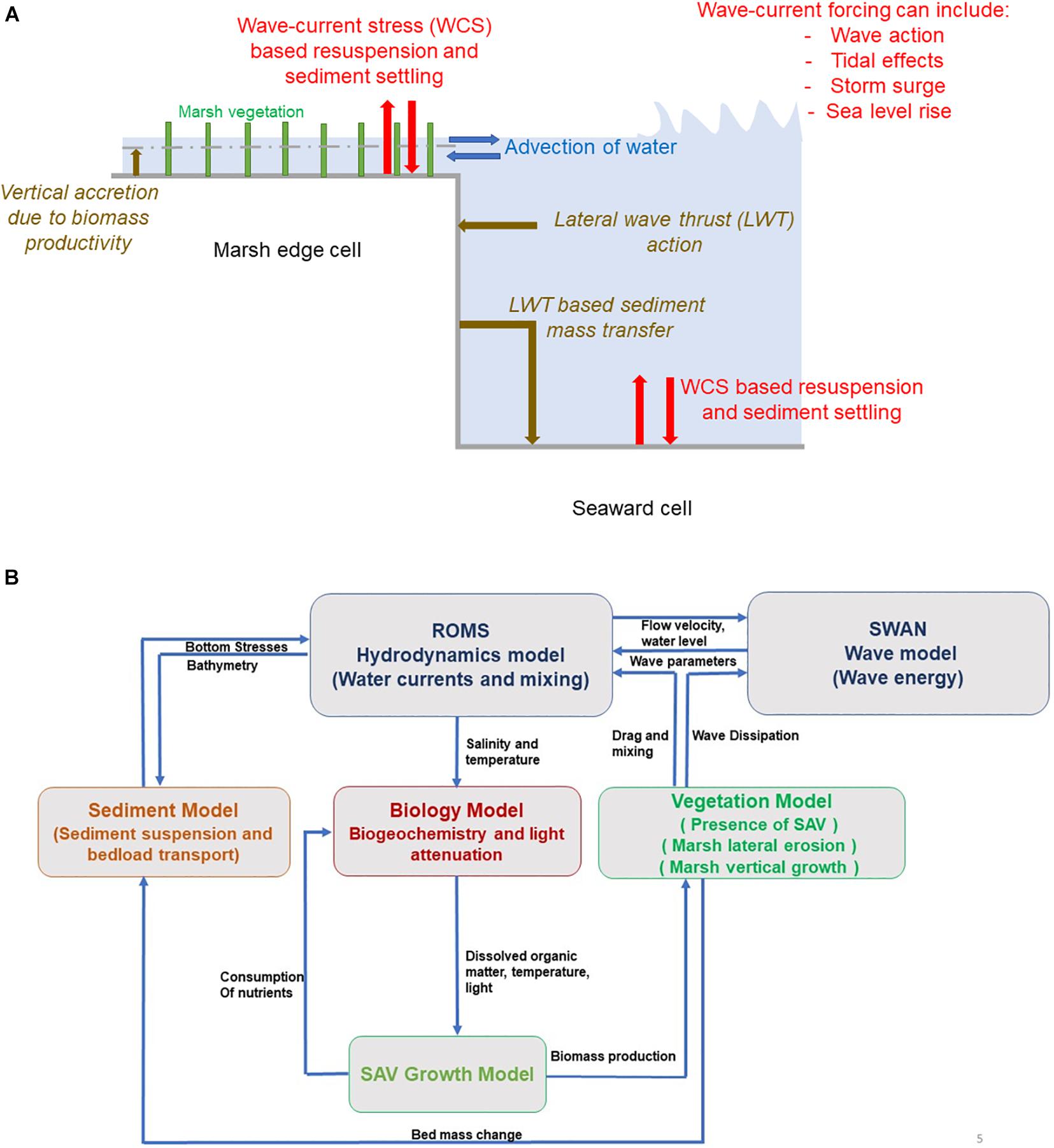
Figure 1. Schematic showing the incorporation of marsh dynamics (lateral wave thrust based erosion and vertical accretion due to biomass production). (A) Newly added processes in the model are shown with brown fonts and brown arrows, (B) flowchart showing the incorporation of the newly added routines within vegetation module in the COAWST model.
Materials and Methods
Modeling Framework
The modeling of marsh erosion due to lateral wave thrust is implemented in the open-source Coupled Ocean-Atmosphere-Wave-Sediment Transport (COAWST) numerical modeling system (Warner et al., 2010). The COAWST modeling framework couples the ROMS (Regional Ocean Modeling System) model for hydrodynamics with a wave model - SWAN (Simulating Waves Nearshore) via the Model Coupling Toolkit (MCT) (Warner et al., 2008). ROMS is a three-dimensional, free-surface, finite-difference, terrain-following model that solves the Reynolds-Averaged Navier-Stokes equations using the hydrostatic and Boussinesq assumptions (Haidvogel et al., 2008). SWAN (Simulating Waves Nearshore) is a third-generation spectral wave model based on the action balance equation (Booij et al., 1999). After a user-defined number of time steps, there is an exchange of water level and depth-averaged velocities from ROMS to SWAN and wave fields from SWAN to ROMS. The Community Sediment Transport Modeling System (CSTMS) model accounts for the 3-D transport of sediment using the bedload and suspended-sediment components. The bedload mass can be updated using a variety of parameterizations that require bed shear stress based on current and wave forcing from the bottom cell. The suspended-sediment is transported by solving an advection-diffusion equation which accounts for a source/sink term that leads to a vertical exchange or settling with the bed. The details of these methods are explained in Warner et al. (2008). The model can represent any number of user defined sediment classes divided into cohesive and non-cohesive types. The amount of sediment stored in the bed is determined through the user-defined properties of each sediment class and sediment bed layer. These properties include bed thickness, sediment density, bed thickness, and bed porosity. In addition to the sediment transport model, the COAWST modeling framework can also account for the change in current and wave dynamics due to the presence of vegetation (Beudin et al., 2017).
Beudin et al. (2017) implemented the physical effects of vegetation in a vertically varying water column through momentum extraction, vertical mixing, and wave dissipation. This allows for the modeling of the impact of marsh vegetation in preventing marsh surface erosion through wave energy dampening and sediment trapping (Möller, 2006; Le Hir et al., 2007; Mariotti and Fagherazzi, 2010). In the current work, we implemented the method to account for marsh edge erosion through the action of lateral wave thrust (LWT) and the method to account for vertical growth of marsh complex due to biomass production. Figure 1B shows the flowchart of the coupled modeling framework of COAWST with the addition of routines for modeling marsh dynamics.
Presence of Marsh Subject to Lateral Wave Thrust
The presence of marsh is defined through a user-defined mask provided to the model as input. A value of 1 corresponds to marsh cells, while a value of 0 is associated with non-marsh regions. Note that this masking operation is independent of the wetting and drying masking framework of COAWST (Warner et al., 2013). The marsh masking can change from 1 to 0 at a given cell once a given amount of user defined marsh retreat due to lateral erosion occurs in the model; this implies that the cell is no longer a part of the marsh. Once the marsh cells are converted to non-marsh cells, they are retained as non-marsh cells.
Computing Lateral Wave Thrust
Once the user specifies the initial marsh mask, the boundary of marsh/non-marsh regions is identified during model runtime. The wave thrust per unit width is calculated by taking the vertical integral of the dynamic wave pressure. The wave thrust is divided into above and below mean sea level components based on the formulations described in the Department of the Army, Waterways Experiment Station, Corps of Engineers (1984). This formulation to compute wave thrust on marsh has been widely utilized in earlier works (Tonelli et al., 2010; Francalanci et al., 2013; Bendoni et al., 2014; Leonardi and Fagherazzi, 2014). Next, we describe the formulation of lateral wave thrust in the model.
First, the above mean sea level component that accounts for the hydrostatic pressure from wind waves (LWTASL) is computed and is defined as:
where ρis the density of water, g is the acceleration due to gravity, and Hs is the significant wave height. Second, the below sea level component, LWTBSL, accounts for the dynamic pressure of wind waves by including the effect of changing water level and is defined as:
where Kp is the pressure-response factor due to water particle acceleration under the effect of wind waves and is calculated as:
whereh is the elevation of the marsh platform at the edge of the scarp with respect to mean sea level, ζ is the water level, and k == , where Lwave is the wave length. Next, the thrust from the two components can be added (Eqs 1, 2) to give the total thrust due to wave attack.
Based on the direction of the waves and grid orientation, the fraction of total thrust that is normal to the marsh cell faced is determined and used in subsequent calculations. All nearest neighbors of a marsh cell can provide LWT (with a maximum of four neighboring cells in the structured grid approach) and then the total wave thrust from all neighboring cells is added to give a total wave thrust on the marsh cell (Supplementary Figure 1 shows the application on LWT on marsh cells).
Next, the effect of water overtopping the marsh on wave thrust is included. Tonelli et al. (2010) showed that the wave thrust reached a maximum when the water level was co-located with the marsh scarp elevation and reduced when waves overtopped the marsh scarp. To account for the change in wave thrust based on water level, various studies have formed different parameterizations (Tonelli et al., 2010; Leonardi et al., 2016b). In the current model implementation, the wave thrust is reduced exponentially as water level increases above the marsh scarp. After modifying the wave thrust based on water level, the resulting wave thrust magnitudes from all the cell faces, i.e., for marsh cells that have multiple edges exposed to the estuary, are summed to obtain a total thrust at each cell center.
Computing Transfer of Sediment Mass Based on Lateral Wave Thrust
The mass of sediment released from marsh cells (mLWT–exportin kg) depends on the lateral wave thrust (LWT in kN/m), marsh erodibility coefficient (kmarshin s/m), grid size (dx in m), and time step size (dt in s).
Based on these factors, the erosion of sediment occurs through a change in bed mass by taking the sediment out from the marsh cell and adding it to the adjacent cell’s bed mass. In the case of a marsh cell surrounded by multiple neighboring grid cells that can provide wave thrust, the sediment change occurs in accordance to Eq. 5. The changes in bed mass modify the bathymetry of the domain leading to a change in bed morphology. Note that the sediment stored in the marsh is assumed to be on the top bed layer, and the model does not account for erosion of material from deeper seabed layers.
Evolution of Marsh Mask and Computing Lateral Marsh Retreat
As mentioned in the previous section, the action of LWT results in a loss of sediment from the marsh. Once enough sediment is exported from the marsh to account for a user-defined reduction in the scarp height, the marsh cell is considered to undergo a horizontal retreat that is equal to the width of the marsh cell. The marsh cell then converts into an open water cell. Specifically, the marsh mask is changed from 1 to 0 for this cell. Note the reduction in scarp height is based on the absolute change of bed thickness. As the marsh cells convert to open water cells, the vegetation in the marsh cells also suffers a dieback and this is simulated in the model by setting the vegetation biomass to zero. Vegetation regrowth is not allowed in marsh cells converted to open water cells. The sediment in the open water cell that was previously a marsh cell can get transported under the action of hydrodynamics.
Accounting for Vertical Growth of a Single Marsh Vegetation Species
The broadly used (Mariotti and Carr, 2014; Kirwan et al., 2016; Carr et al., 2018, 2020; Mariotti, 2020) growth model formulation is adapted from Morris et al. (2002) following the formulation of Kirwan and Murray (2007) where vegetation rapidly adjusts to changes in elevation and as such biomass can be calculated as a function of marsh cell depth below a Mean High Water (MHW). In these two studies, the biomass productivity formulations were based on measurements from S. alterniflora. Biomass productivity (Bpeak)is based on a parabolic biomass curve where the upper (Dmax)and lower limits (Dmin) of the parabola are a function of MHW and is defined as:
where Bmax is the optimal biomass in kg m–2yr–1 that is a user input where
and where MTR is the mean tidal range and is assumed to be MTR = 2MHW. cff in the denominator of Eq. 6 is a scaling factor that does not allow the value of Bpeak to exceed a maximum value of Bmax set as a user input of 2.5 kg m–2yr–1 and is defined as:
Meanhighwater is calculated internally as a moving average over user defined days by keeping a track of the maximum water level in a day. The upper and lower limits correspond to reference depths where the macrophyte survives and leads to accretion of biomass (McKee and Patrick, 1988). The integrated per year amount of below ground biomass (AMC) corresponding to 180 days of growth in kg m–2yr–1 is calculated as:
where nugp is the fraction of below ground biomass set to be an input of 0.0138 day–1 and tdaysgrowth is set to be 180 days. tdaysgrowth represents a growing period for marsh vegetation within the marshes in Barnegat Bay. The effective biomassRref in kg m–2yr–1 after accounting for recalcitrant carbon is calculated as:
where chiref is the fraction of recalcitrant Carbon set to be an input of 0.158. The model choice of nugp, tdaysgrowth, and chiref are all based on Mudd et al. (2009). The rate of vertical growth due to biomass production over marsh cells (m/year) is calculated from Rref using:
where mbulk–dens is the bulk density of marsh organic matter. The vertical growth rate is used to calculate vertical accretion and is then converted to a change in bed mass in marsh cells.
Model Simulations
The mechanistic processes that model marsh dynamics in the COAWST framework were tested by simulating two idealized domains and realistic domains of two creeks within the Barnegat Bay. The first idealized setup is modeled with constant wave statistics over the entire domain to verify the implementation of the lateral wave thrust (LWT) magnitude with previous work of Tonelli et al. (2010). The second idealized domain is setup with a high resolution grid in east-west direction to model the mechanism of lateral retreat due to LWT action at marsh edge; that leads to conversion of marsh edge to open water cells. Next, the simulations involve the application of the Barnegat Bay setup of Defne et al. (2019) followed by modeling of two creek systems (Reedy and Dinner Creek) with distinct tidal ranges to show the modeled processes of LWT action and vertical growth in realistic domains. The details of the modeled domains are explained in the following sections.
Idealized Domain to Formulate and Verify Lateral Wave Thrust
The numerical experiments of Tonelli et al. (2010) calculate maximum wave thrust for three different wave heights and provides a dataset to verify the implementation within the current model. The setup of the domain involves a basin of 10 by 1 km rectangular domain leading to a grid resolution of 100 by 50 m with a depth of 1.3 m. The plan view of the domain is shown in Figure 2A and the variation in bathymetry along the channel is shown in Figure 2B. The marsh complex is located at an elevation of 0.1 m above mean sea level. The elevation of 0.1 above MSL is based on the numerical experiments of Tonelli et al. (2010) where the mean water level of the numerical experiments is set to 1.4 m above the bottom of the domain. The model is forced by oscillating the water level on the northern edge with a tidal amplitude of 0.5 m and a period of 12 h. The waves are imposed in the entire domain to have a constant wave height and wavelength. The waves impinge at a 0 degrees angle with respect to the northern boundary with a period of 2 s. Because the waves are constant in the domain, this simulation remains uncoupled (no wave model). The constant waves in the domain are generated by providing bulk wave statistics in an input file to match the wave conditions of Tonelli et al. (2010). The ROMS barotropic and baroclinic time steps are 20 and 1 s, respectively. The wave height is varied to find the variation of maximum wave thrust with water level and compared with the results from Tonelli et al. (2010). The model setup is run for two tidal cycles allowing computation of the influence of varying water levels on the maximum lateral wave thrust. Three different scenarios of wave height are simulated by forcing the northern boundary with heights of 0.2, 0.3, and 0.4 m.
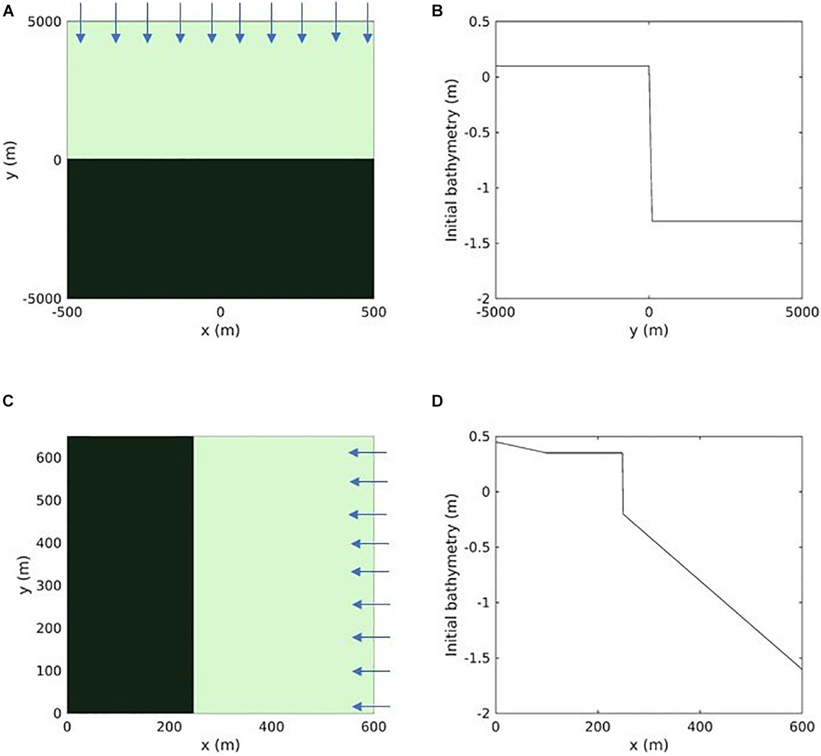
Figure 2. Idealized case to formulate lateral wave thrust: (A) Planform view and, (B) Initial bathymetry for 100 m resolution domain. High resolution idealized case to test the marsh lateral retreat formulations: (C) Planform view and, (D) Initial bathymetry for 1 m resolution domain. Estuary and marsh coverage are shown by light and dark green colors, respectively, in the planform view and arrows point toward the direction of hydrodynamic forcing.
High Resolution Idealized Domain to Test Marsh Lateral Retreat Formulations
An idealized test case with higher spatial resolution is developed to test the model’s ability to simulate marsh lateral retreat on the order of 1 m. Figure 2C shows the plan view of the model domain that is 600 m long and 650 m wide with a grid resolution of 1 and 25 m in the cross-shore and along-shore directions, respectively. A grid resolution of 1 m allows for modeling a realistic case of retreat of marsh cells that occurs from a monthly to annual time scale while also simulating short timescale dynamics with a timestep of 1 s. The initial bathymetry consists of a maximum depth of 1.6 m corresponding to the seaward side (eastern boundary) that tapers to 0.2 m depth spanning over 353 m of the domain. Beyond that, a fixed elevation of 0.35 m describes the start of the marsh complex. The variation in bathymetry along the length of the channel at a cross-section (y = 325 m) is shown in Figure 2D. The marsh complex in the setup is vegetated and one sediment class is used for the entire domain with marsh vegetation and sediment properties presented in Supplementary Table 2. The model is forced by oscillating the water level on the eastern edge with a tidal amplitude of 0.5 m and a period of 12 h. Waves are also imposed on the eastern edge with a height of 0.3 m, directed to the west (90 degrees) with a period of 6.28 s. The northern and southern boundaries of the domain are closed. The bottom boundary layer roughness is increased by the presence of waves that produce enhanced drag on the mean flow (Ganju and Sherwood, 2010). The turbulence model selected is the k−ε scheme (Warner et al., 2005). The complete list of model parameters is shown in Supplementary Table 2.
To initialize the model, the simulation is setup without the action of LWT on the marsh domain. This allows for erosion to occur from the elevated platform due to only wave-current stresses (WCS). The model is run until the marsh platform topography has stabilized. The simulations are then restarted with the introduction of marsh mask and inclusion of LWT routines. After that the marsh edge erodes under the combined effect of WCS and LWT. These simulations are continued until the marsh edge cell retreats and a second marsh edge cell is formed using the methods described above.
Barnegat Bay Creek Simulations
We test the combined effects of dynamic sediment transport, lateral wave thrust induced erosion, and vertical growth due to biomass productivity using two different simulations involving marsh complexes within Forsythe National Wildlife Refuge and the Barnegat Bay (BB) estuary. The COAWST BB model was developed and applied by Defne et al. (2019). We use the same setup of the BB domain (Figure 3A) and simulated the model grid for the period of May, 2015. The tidal forcing is generated from the ADCIRC product (Szpilka et al., 2016) and wind forcing is generated from the 3-hourly North American Mesoscale Forecast System product (NCEP NAM, 2020). Three estuarine sediment types and one marsh sediment class were utilized following the study of Defne et al. (2019). The marsh and submerged aquatic vegetation (SAV) presence along with their properties in the estuary was determined using the model development of Donatelli et al. (2018).
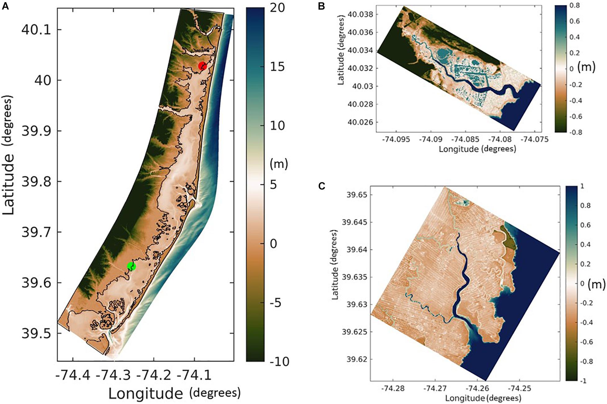
Figure 3. Colormaps of bathymetry with negative values representing elevation above MSL and positive values representing depth below MSL from (A) Barnegat Bay grid from Defne et al. (2019) with red and green circles showing the location of Reedy and Dinner Creek observations, respectively (Ganju et al., 2017), (B) Reedy Creek, and (C) Dinner Creek grids.
We used the model output from the BB simulation to provide the hydrodynamic (Supplementary Figure 4) and sediment forcing (water level, barotropic and baroclinic velocities, waves, and suspended sediment) to provide hourly boundary forcing conditions for the two creek grids. The grid dimensions for the two marsh complexes are 132 × 388 points and 599 × 539 points, at 5-m resolution with 7 vertical sigma layers, for Reedy Creek and Dinner Creek, respectively (Figures 3B,C). The northern, southern and eastern boundaries of the two domains remain open to BB domain forcing, while the western boundaries are closed. Initial model bathymetry is obtained from the CoNED topo bathymetric model for New Jersey and Delaware (OCM Partners, 2021). The bathymetry in the channel is modified to be 1 m in the Reedy creek domain and 2.3 m in the Dinner creek domain to match the observed bathymetry of Suttles et al. (2016). The marsh elevation from CoNED for the RC domain is adjusted by 0.1 m to field measurements (real time kinematic global positioning, Quirk, 2016) and comparison to local mean sea level. A similar elevation shift (∼0.1 m) is seen in the local mean sea level computed from a decade long water level time series at the nearby Mantoloking station. For the DC domain, we retained the marsh elevation as provided by the CoNED model. For each domain, the cells with marsh mask are based on the updated National Wetland Inventory delineation for BB (Defne and Ganju, 2016) and defined in the model as all the cells covering the vegetated areas or cells under a depth of 0.1 m. The same area is used to specify marsh vegetation properties (Supplementary Table 3). The suspended marsh sediment class in BB domain is exchanged with the creek domains as part of the open boundary forcing. In addition to this, two more marsh sediment classes, organic and inorganic, were introduced in the creek simulations. In the simulations, the organic marsh class can accumulate only through vertical growth processes. This allows for distinguishing the sources of sediment on the marsh complex that could be derived from either organic (first) or inorganic (second) class of sediment or the inorganic (third) class available from the BB domain boundary. Supplementary Table 3 specifies the properties of the sediment classes, marsh/estuarine bed, and marsh vegetation used during the creek simulations. At the boundary of RC domain, the maximum and mean suspended sediment concentration (SSC) corresponding to the finest estuarine sediment class are 15 and 3 mg/L, respectively, while the maximum and mean SSC for the coarsest estuarine sediment are 0.2 and 0.002 mg/L. At the boundary of DC domain, the maximum and mean suspended sediment concentration (SSC) corresponding to the finest estuarine sediment class are 38.6 and 13 mg/L, respectively, while the maximum and mean SSC for the coarsest estuarine sediment are 3.9 and 0.45 mg/L. In the creek simulations, the ROMS time step is 1 s, while the SWAN time step and the coupling interval between ROMS and SWAN are 20 min. The friction exerted on the flow by the bed is calculated using the bottom boundary layer formulation (Warner et al., 2008). The bottom boundary layer roughness is increased by the presence of waves that enhance drag on the mean flow (Ganju and Sherwood, 2010). The vegetative drag coefficients (cD) in the flow model and the wave model are set to 1. The bed roughness is set to z0 = 0.015 m, which corresponds to a mixture of silt and sand (Soulsby, 1997). The turbulence model selected is the κ − ε scheme (Warner et al., 2005).
Results
Verification of Lateral Wave Thrust Calculation
Under the influence of varying water levels in the model setup described in Section “Idealized Domain to Formulate and Verify Lateral Wave Thrust,” the maximum LWT is computed in three different scenarios corresponding to wave heights of 0.2, 0.3, and 0.4 m (Figure 4). The use of constant wave forcing in the current approach ensures that we can simulate wave conditions similar to the numerical experiments of Tonelli et al. (2010). LWT increases with increasing wave heights. As the water level goes above the marsh scarp, the LWT starts to reduce exponentially because water runs on top of the marsh scarp. LWT peaks when the water level elevation is equal to the scarp height. As the water level drops, the integrated LWT starts to decrease over the marsh scarp. The pattern of LWT variation with depth above bottom is consistent with the numerical experiments from Tonelli et al. (2010). However, because the present approach relies on bulk wave statistics to parameterize LWT (section “Computing LWT”) the degree of non-linearity is much lower in LWT variation. On the other hand, the numerical experiments of Tonelli et al. (2010) capture the non-linear wave dynamics in their modeling methodology and calculate LWT directly by integrating pressure forces over the marsh scarp.
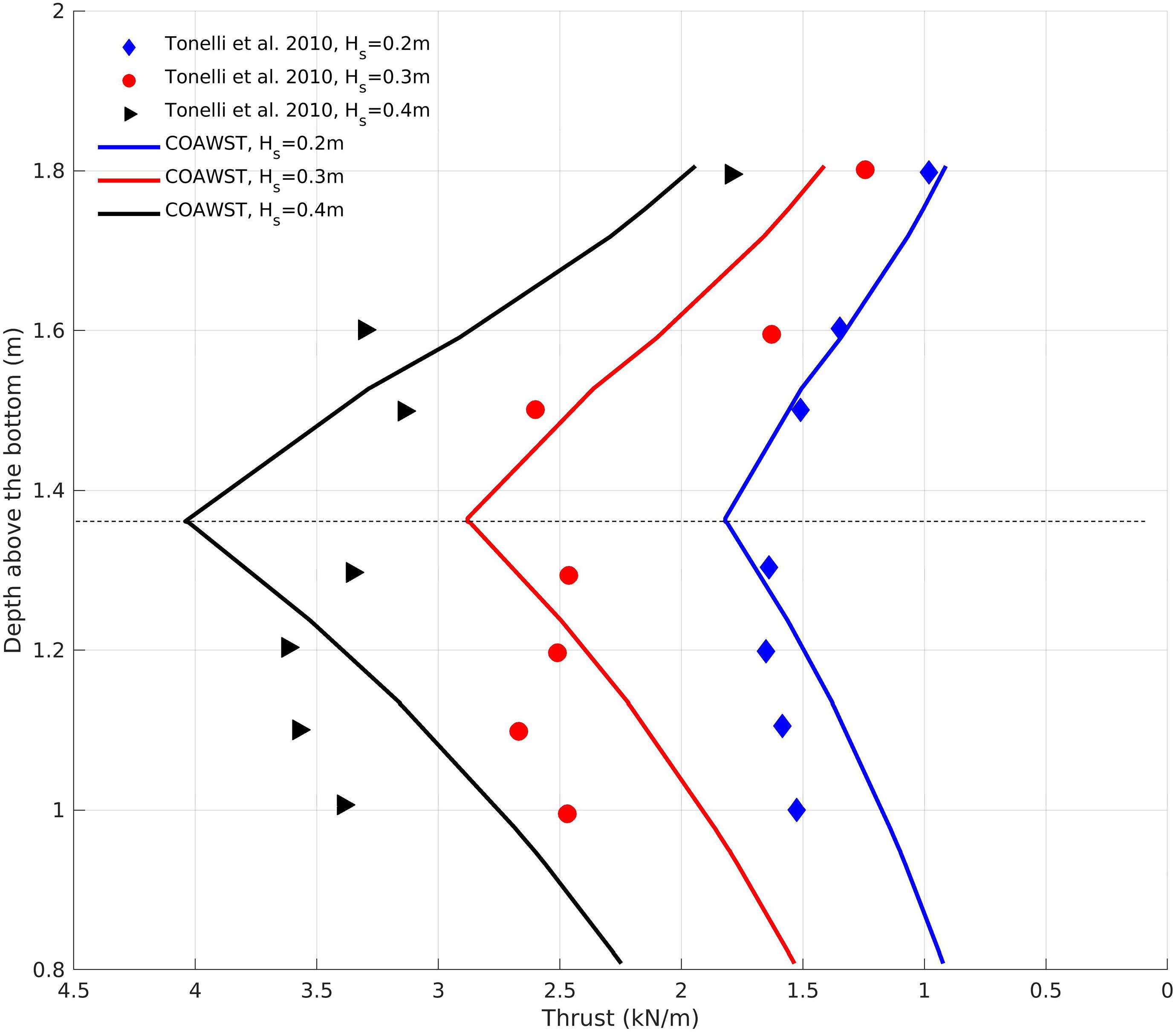
Figure 4. Lateral wave thrust comparison for different incident wave heights (0.2, 0.3, and 0.4 m) between the numerical data of Tonelli et al. (2010) and COAWST model. The marsh complex is located at a depth above the bottom of 1.4 m.
Export of Marsh Sediment and Marsh Retreat (HR Grid)
Initially, model setup is simulated without the action of LWT while an elevated platform starts to erode under the action of combined WCS until the bathymetry at the edge of the elevated platform is stable. The transect at x = 248 m shown in Figure 5A corresponds to the cell that dropped the most in elevation only due to WCS (marsh edge pre-LWT) and provides the topography at the end of 351 days, where the marsh edge pre-LWT had a change in elevation from 0.35 to 0.02 m. The cells at or below the depth of 0.02 m are considered open water cells and the remaining cells in the cross-channel direction (east to west direction) that still maintain an elevation greater 0.02 m in the domain are masked to be marsh cells. At this time, the edge of the marsh complex is at an elevation of 0.27 m starting from the marsh edge (x = 247 m, referred to as “pre-LWT” in Figure 5A). The user defined scarp height to erode the edge due to the lateral wave action is also set to this elevation (i.e., 0.27 m with the marsh edge located at x = 247 m). After setting the marsh mask for the marsh complex, the simulation is restarted with the effect of LWT included.
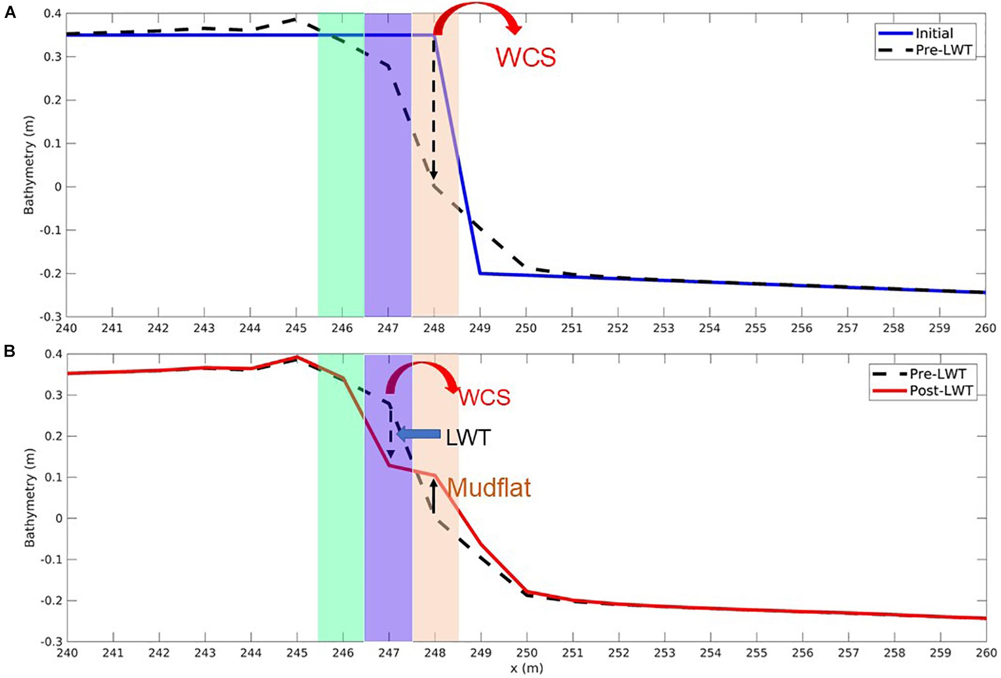
Figure 5. Cross-shore profile showing topographic change from the high resolution (1 m) idealized domain: (A) Initial and final stabilized bathymetry pre-LWT following the effects of wave-current stress (WCS) only and before lateral wave thrust (LWT) is introduced (at the end of 351 days), (B) pre-LWT and post-LWT until the conversion of marsh cell to non-marsh cell (after 567 days). The shaded regions brown, blue, and green indicate the presence of marsh edges (pre-LWT at x = 248 m until 351 days, post-LWT marsh edge 1 at x = 247 m from 351 to 567 days and post-LWT marsh edge 2 at x = 246 m from 567 days until the end of the simulation set to 665 days), respectively.
Following the WCS-only run, the model is resumed with the LWT formulations. For the same transect described in the previous paragraph (marsh edge 1 at x = 247 m), the marsh edge drops to an elevation of 0.13 m after 216 days. After 216-days of model run, the marsh edge (x = 247 m) drops to an elevation of 0.13 m. The combined processes of WCS and LWT change the bed thickness to the user defined scarp height of 0.27 m. Based on the retreat formulation (section “Evolution of Marsh Mask and Computing Lateral Marsh Retreat”), the marsh edge cell (marsh edge 1 post-LWT at x = 247 m) converts to an open water cell, forming a unvegetated mudflat adjacent to the marsh (Figure 5B). Due to the retreat of the marsh edge cell at x = 247 m, a new marsh edge cell is created at x = 246 m (referred to as “marsh edge 2 post-LWT” at x = 246 m).
A change in the bed thickness of the sediment bed in the cross-channel direction during the erosion of marsh edge 1 post-LWT is shown in Figure 6A. The lowering of marsh complex elevation results in a lower vertically integrated wave thrust and therefore the total wave thrust decreases over time (Figure 6B). After marsh edge 1 post-LWT gets converted into an open water cell, the new marsh edge (marsh edge 2 post-LWT) is influenced by LWT action. A similar pattern is observed in the change in daily flux out of the marsh edge cells (Figure 6C), where the decrease in wave thrust with lowering elevation results in lower flux out of the marsh edge cells.
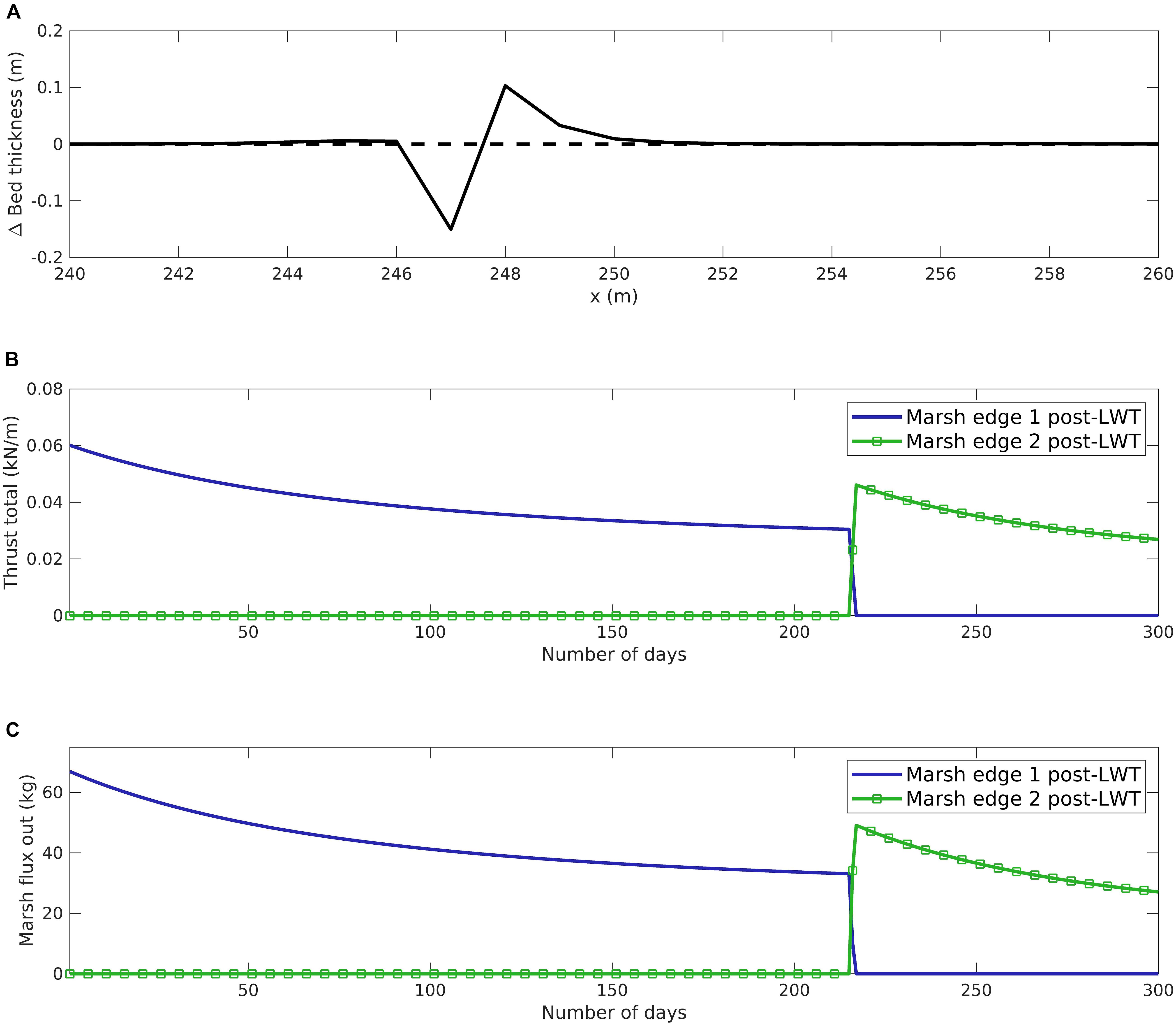
Figure 6. Marsh shoreline erosion results from high resolution (1 m) idealized domain: (A) Initial and final bed thickness change at a cross-section. (B) Averaged daily lateral wave thrust on marsh edge. (C) Averaged daily flux of sediment out of the marsh edge cells.
Creek Simulations at Barnegat Bay
We tested the combined dynamics of lateral wave thrust (LWT)-based erosion and vertical growth due to biomass productivity using two different simulations involving creeks in the Barnegat Bay estuary. Figures 7A,B show the spatial pattern of LWT that is summed over the 31-day long simulation period for each of the two domains. In both domains, the cells closer to the open bay experience a higher LWT compared to the cells inland. The spatial variation in LWT is explored by looking at two points in the RC domain (Figure 8A). The first point close to the open bay is referred to as “Bay point” and the second point inland of the RC channel is referred to as “Inland point.” Figure 8B shows the significant wave height (Hs) generated by winds at the points referenced in Figure 8A. The root-mean-square (rms) Hs over the 31-day period for the bay point is 0.03 m while rms Hs for inland point is nearly zero. Other than Hs, the wave direction impacts the formulation of LWT as it only allows for the normal component of waves (after accounting the orientation of the grid) to provide wave thrust from adjacent wet cells to the dry marsh edge cells. The bay point receives a higher integrated LWT over the 31-day period with a rms LWT of 0.034 kN/m while rms LWT for inland point is nearly zero, highlighted in Figure 8C.
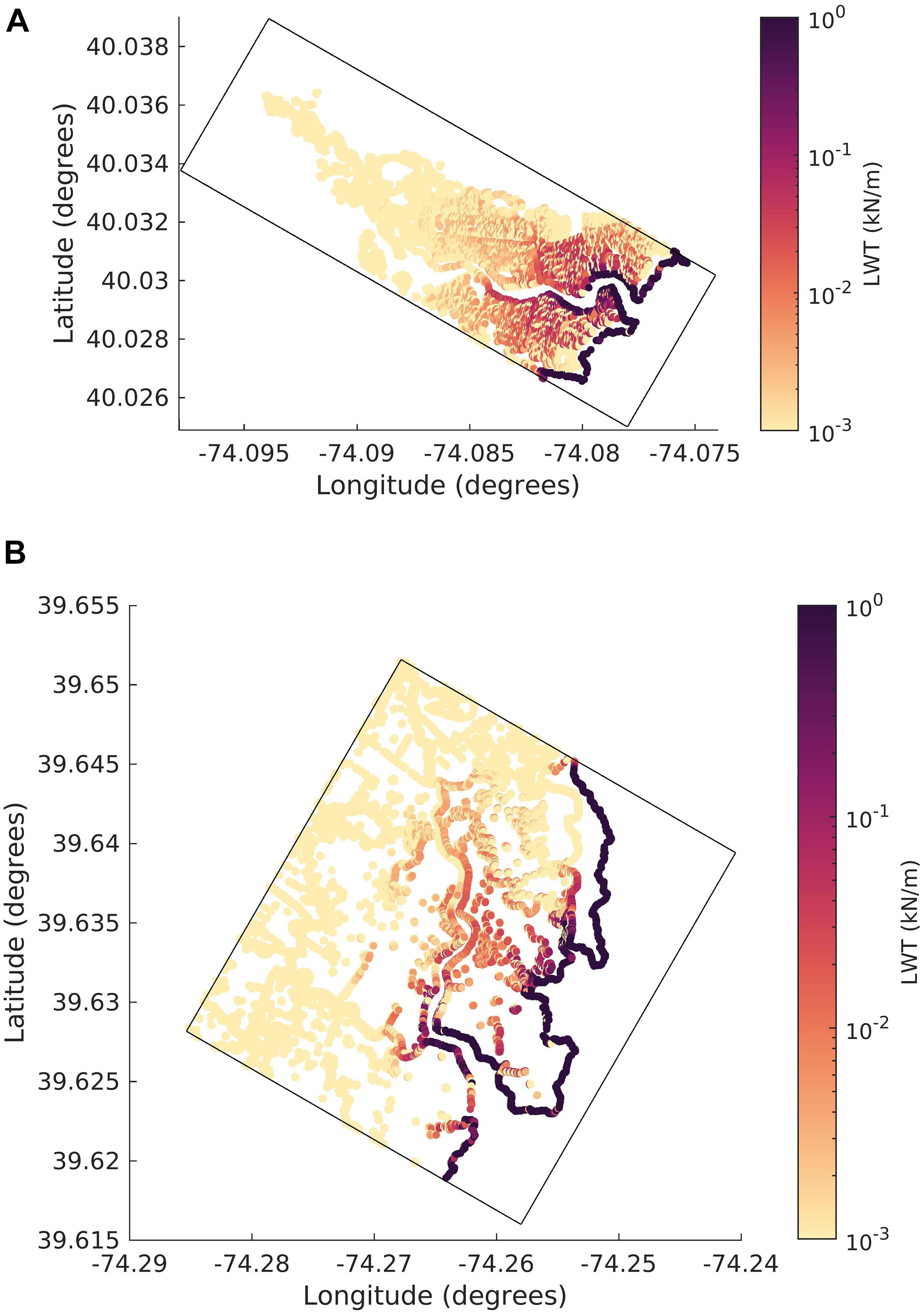
Figure 7. Integrated lateral wave thrust map integrated over 31 days. (A) Reedy Creek and (B) Dinner Creek domain.
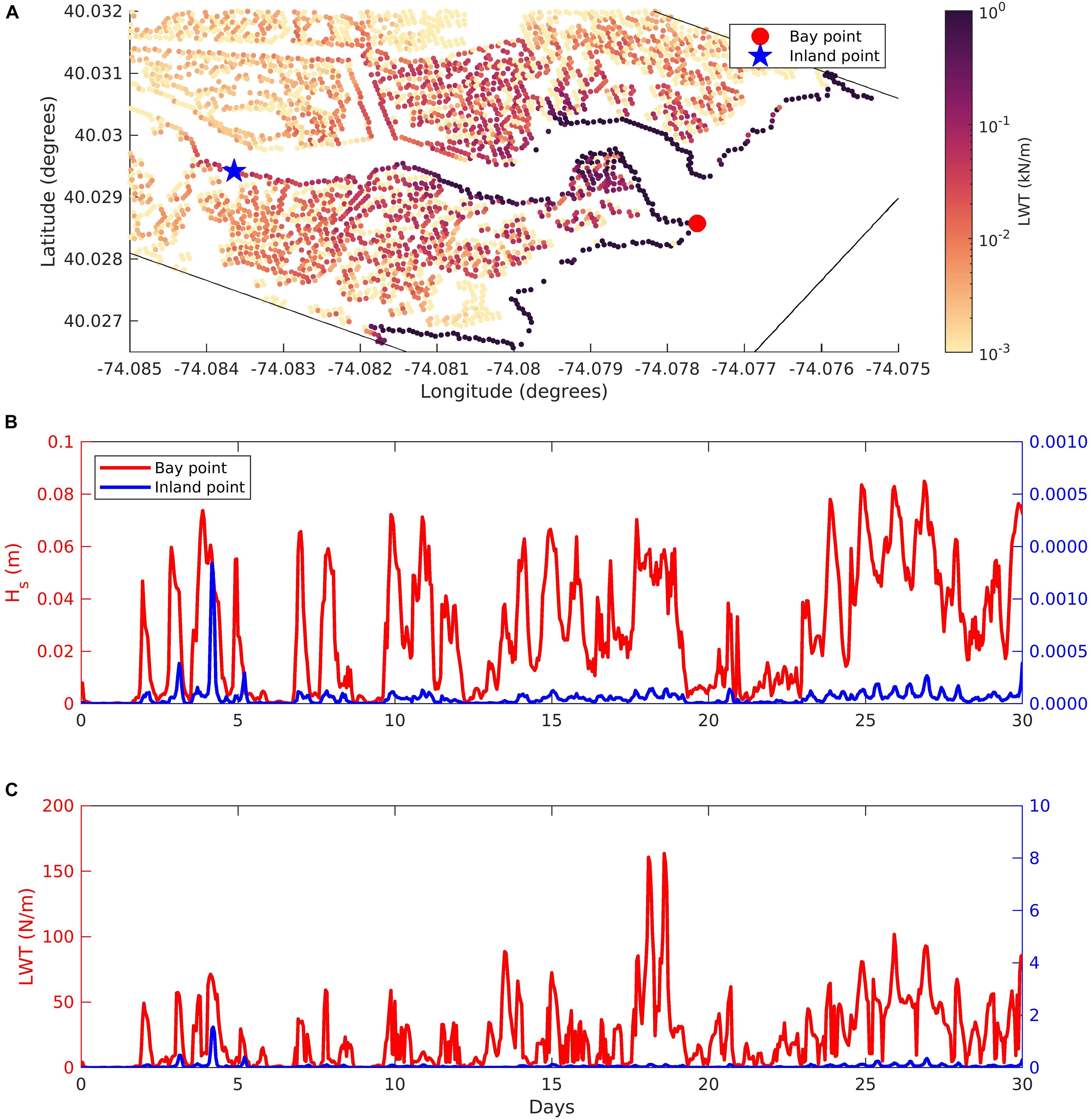
Figure 8. (A) Reedy Creek domain showing integrated lateral wave thrust (LWT) and indicating the location of bay (red circle) and inland points (blue star) for the time series plots of (B) significant wave height (Hs) and (C) lateral wave thrust (LWT). The left “y” axis in (B,C) correspond to bay point and right “y” axis corresponds to the inland point.
Next, we analyze the vertical growth rate (VGR) of organic sediment due to biomass productivity at the end of the simulation period for the two creek domains in Figure 9. The difference in VGR between the two domains is relatively small. The VGR increases north of the DC channel more than in the southern end while remaining high along the channel for the RC domain.
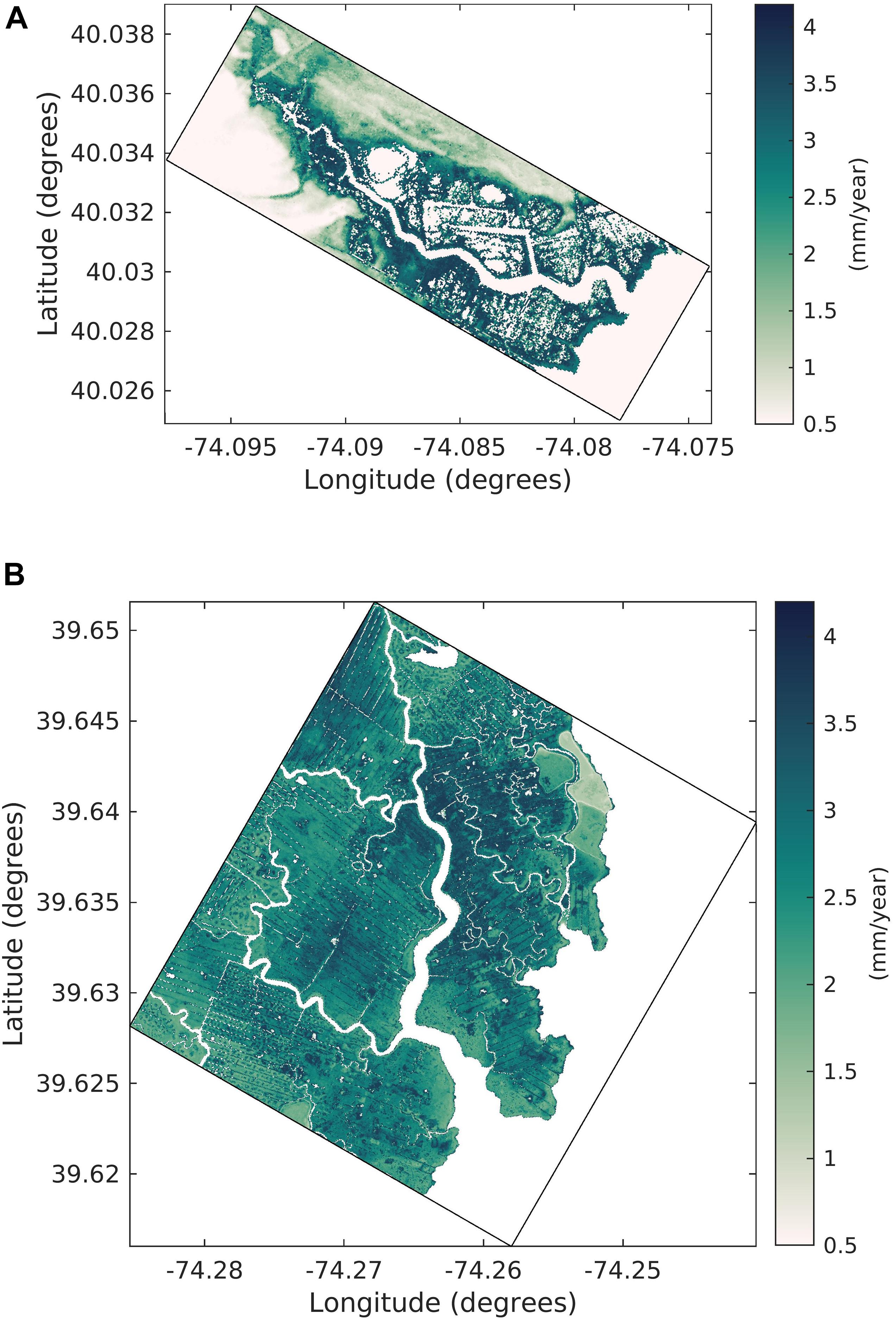
Figure 9. Vertical growth rate due to biomass productivity at the end of the simulation (A) Reedy Creek and (B) Dinner Creek domain.
We use two points (inland and at the bay end) from the RC domain to understand the reasons for spatially varying VGR (Figure 10A) and the reference datums that describe the upper (Dmin) and lower (Dmax) limits of the parabolic growth curve along with the elevation of the two chosen points (Figure 10B). The rolling average to get Dmin and Dmax employs a user-defined period of 7 days. The bay point is at a lower elevation around 2 cm while the inland marsh point is 12 cm above datum. Following the parabolic formulation, the highest amount of growth occurs when the cell elevation is midway between the upper and lower limits of the parabola and decreases away from the middle datum. In Figure 10B, the elevation of the bay cell is close to Dmax while the elevation of inland cell is located close to the midway point between Dmin and Dmax, providing an optimum elevation for biomass productivity within the salt marshes. Consequently, at the end of the simulation period, the inland cell grows at a 3.6 mm/year rate, higher than the 2.1 mm/year growth rate for the bay point. It should be noted that the VGR per year is computed based on a monthly calculation and would vary once the effects of seasonality on biomass productivity and on hydroperiod parameters are considered in a year long simulation. To compare the LWT and VGR pattern between the two creeks, we extracted the points along the channel from the two domains and categorized them into eastern and western points for the two domains (Figures 11A,B). For both the domains, the orientation of the waves results in a higher integrated LWT at the eastern end of the channels (Figures 11C,D). Due to the open mouth of the DC channel, the maximum integrated LWT over the 31-day period is higher for the eastern end of the DC domain (74.1 N/m) compared to the eastern end of RC domain (60.4 N/m). Between the western ends, integrated LWT is higher for the RC domain (16.4 N/m) compared to the DC marsh complex (12.2 N/m). In addition, the effect of LWT extended to a distance of 1000 m for the DC domain compared to 200 m for the RC domain. A comparison of VGR for the two domains made by analyzing the VGR variation with elevation show the mean elevation for the eastern and western ends of DC domain is higher (12.6 and 14.7 cm, respectively) compared to RC domain (11.9 and 13.9 cm, respectively). In addition, the tidal range for the DC domain is 70 cm while the RC domain is 20 cm. The combination of higher elevation marsh cells along with increased tidal range provides a larger envelope for the parabolic formulation growth curve for the DC domain compared to the RC domain (Figures 11E,F).
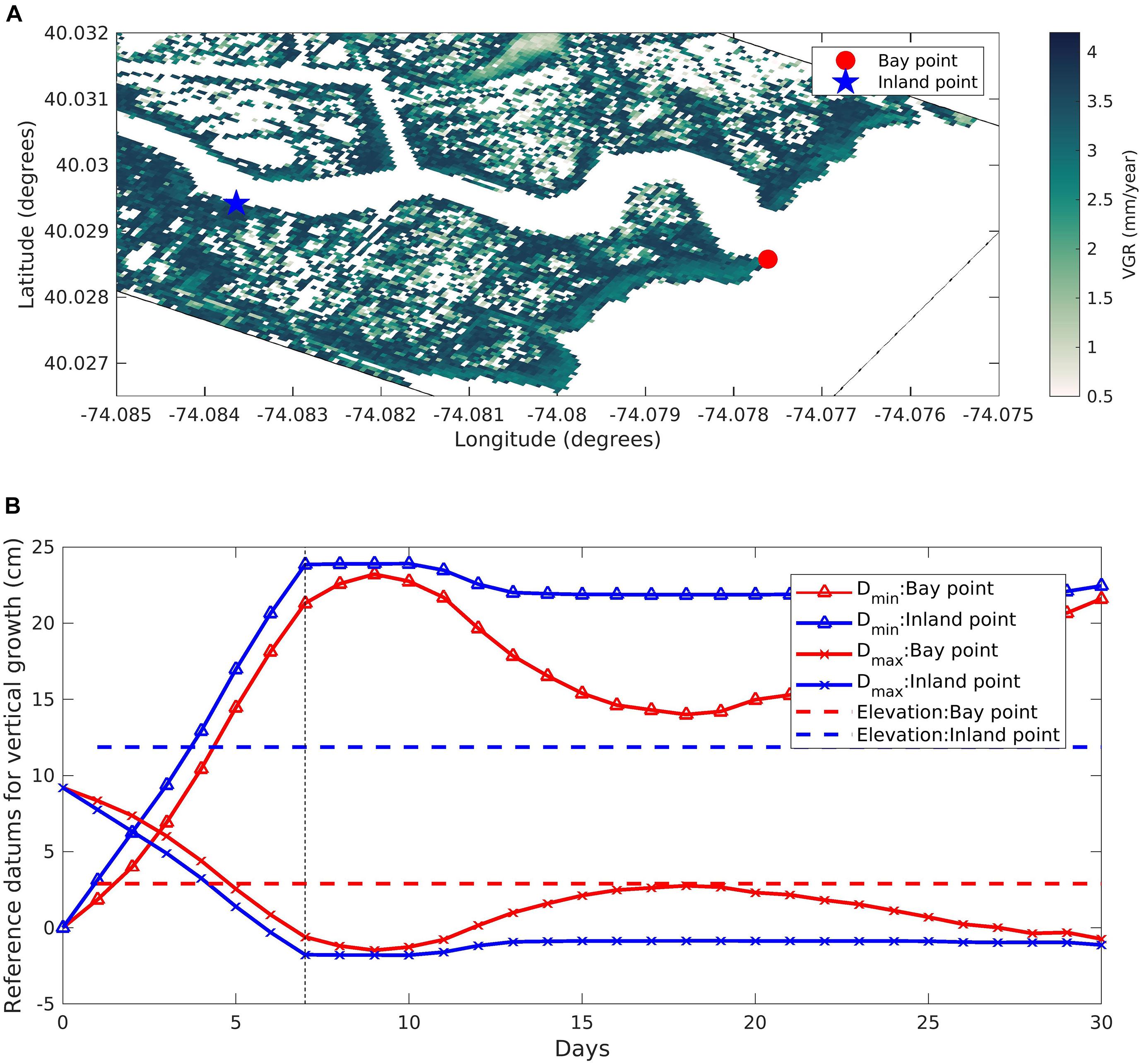
Figure 10. (A) Zoomed in Reedy Creek domain showing the colormap of vertical growth rate (VGR) due to biomass productivity at the end of the simulation with the location of bay (red circles) and inland points (blue star), with (B) time series of reference datums for vertical growth rate at Bay and Inland point.
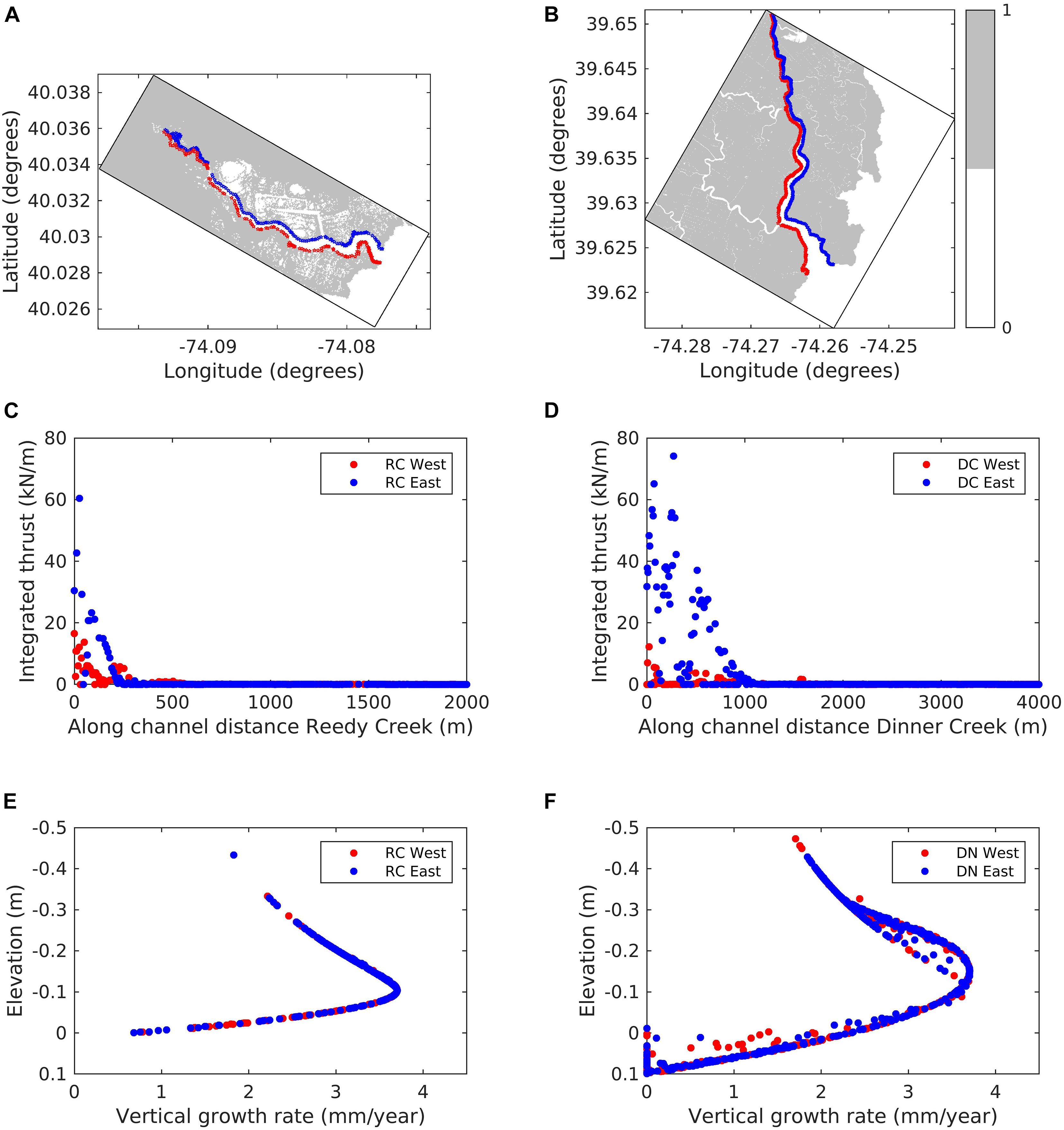
Figure 11. Extraction of shoreline points along the tidal creek channel on the east (red) and west (blue) sides of the (A) Reedy Creek (RC) and (B) Dinner Creek (DC) domains with marsh shown [Marsh mask = 1 (gray contour) indicates marsh presence]. Graph show the along channel variation of integrated lateral wave thrust (LWT) for both the eastern and western sides of (C) RC and (D) DC domains; and vertical growth rate (VGR) variation with marsh elevation (negative elevation refers to points above MSL) for shoreline points located on the eastern and western sides of (E) RC and (F) DC domains at the end of the simulation.
Next, we analyze the amount of sediment deposition from various processes in the two domains (Figure 12). This includes the amount of sediment deposition due to biomass productivity (Figures 12A,B), inorganic marsh sediment (Figures 12C,D) and inorganic estuarine sediment (Figures 12E,F) deposited from the process of tides and waves (hydrodynamic forcing) overtopping the marsh cells. In the RC domain the organic sediment is accumulated (Figure 12A) following the pattern of spatial changes in VGR due to biomass productivity observed in Figure 9A. The inorganic marsh sediment deposited from hydrodynamic forcing is limited to only a few cells (Figure 12C). The inorganic estuarine sediment deposited over the marsh is significantly higher in the southern end of the channel and decreases north of the RC domain (Figure 12E). Similar to the RC domain, the organic sediment accumulation follows the pattern of VGR for the DC domain (Figure 12B). It is observed that a larger number of cells accrete inorganic marsh sediment due to the hydrodynamic forcing (Figure 12D) and there is a larger deposition of inorganic estuarine sediment toward the northern end of the channel in the case of DC domain (Figure 12F).
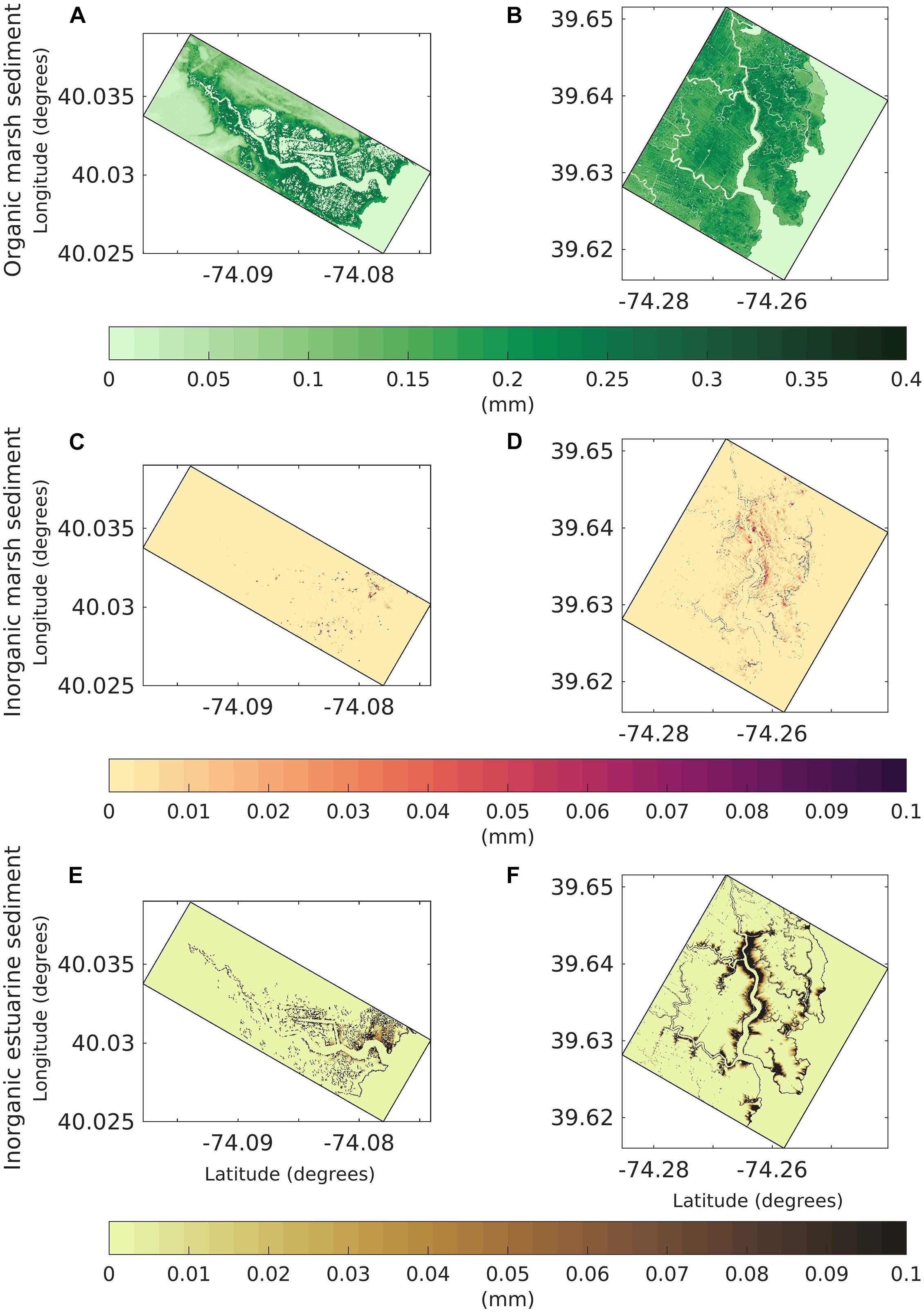
Figure 12. Distribution maps of the modeled sediment deposition by type for both the Reedy Creek (RC) and Dinner Creek (DC) marsh complexes at the end of the simulation. Organic marsh sediment depth for the (A) RC and (B) DC domain. Inorganic marsh sediment depth for the (C) RC domain and (D) DC domain. Inorganic estuarine sediment for the (E) RC domain and, (F) DC domain. The colorbar is common to both domains for each sediment class.
Discussion
Relative Importance of Marsh Dynamic Processes
Numerical models used to assess salt marsh trajectory typically incorporate a subset of the relevant physical processes (Fagherazzi et al., 2012; Ganju, 2019). More robust models must be developed to simultaneously account for lateral and vertical processes, in addition to dynamic sediment transport within the surrounding estuary, tidal channels, and intertidal flats. For example, vertical biogenic models (Morris et al., 2002; Alizad et al., 2016) alone will neglect the import of estuarine sediment along tidal channels that aid in landward deposition, while abiotic sediment transport models (Temmerman et al., 2005; Donatelli et al., 2018; Defne et al., 2019) neglect vertical response of the marsh to tidal levels. The modeling framework developed and applied here considers the dominant dynamic, lateral, and vertical processes in a coupled geomorphic context. This is necessary to properly evaluate marsh response to future climatic (morphodynamic) changes.
Within this modeling framework, there are three distinct sources of sediment that contribute to marsh development and deterioration. In addition to the process of sediment transport induced from wave-current stress, the present framework incorporates (1) the processes to account for the organic material accumulated due to biomass production and (2) the lateral wave thrust action leading to erosion of sediment from the marsh onto the estuary (Figure 1A). Table 1 shows the total mass of sediment deposited over all the marsh grid cells in the Reedy and Dinner Creek simulations. The largest source of sediment to the marsh in terms of mass in both creek simulations is the inorganic estuarine sediment (61% of deposition over the RC marsh and 94% of deposition over the DC marsh). Meanwhile, the total mass of inorganic marsh sediment (from marsh edge erosion) represents 25% of the total sediment accumulation over the marsh in RC and 3.7% in DC. The total mass accumulated over the Dinner Creek marsh is 45 times larger than the mass accumulated over Reedy Creek. This is consistent with the more energetic tidal currents and wave climate present in the Dinner Creek domain.
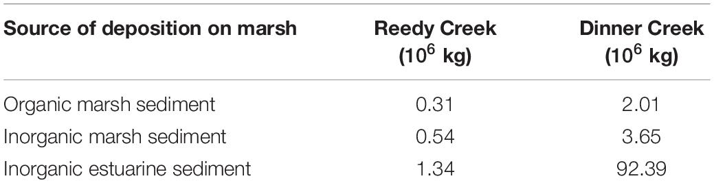
Table 1. Amount of total sediment deposition summed over all grid cells in each marsh complex.
Figure 13 shows the extent of coverage of marsh grid cells from the three sources of sediment in the two creek domains More than 90% of the area of deposition in the marsh complex in both domains is dominated by the organic marsh sediment (Figure 13). In the entire RC marsh complex, the coverage of inorganic marsh sediment is over 0.4% of the marsh while the area covered in the DC marsh complex is 0.97%. In the DC domain, the inorganic estuarine sediment covers (5.7%) of the area compared to 5.3% in the RC domain (Figure 13). The comparison between the two creek domains shows that a larger area of marsh complex in the DC domain gets affected by the inorganic marsh and estuarine sediment compared to the RC domain. This can be attributed to the higher LWT and higher tidal forcing in the DC domain that leads to a higher availability of marsh and estuarine-derived inorganic sediment transport. The larger tidal range, and higher velocities therefore in the DC domain is also responsible for an increased accretion in the north end of the DC channel, where suspended-sediment concentrations are large due to advection (Figure 13B). When only the marsh areas dominated by the two inorganic sources of sediment (marsh and estuarine) are considered, the estuarine sediment dominates over 75% of those locations in RC domain. In contrast, 50.4% of the marsh cells on the DC marsh complex are dominated by inorganic sediment have a predominant marsh-edge erosion sediment source. These results mirror the higher tidal and wave energy in the southern part of Barnegat Bay, where sediment fluxes are larger leading to higher sediment load (Ganju et al., 2014) and likely increasing estuarine sediment transport onto the marsh platform. Organic accumulation dominates over most of the interior marsh plains, due to limited ability of sediment to be advected there given low or negligible water velocities and settling of sediment (Coleman et al., 2020). The large area of accretion due to biomass production shows that this process is the principal mechanism through which marsh complexes vertically accrete similar to the observations (Neubauer, 2008; Morris et al., 2016). The inorganic sediment (both estuarine and marsh) gets redeposited close to the marsh edge with a reduced deposition in the interior of marsh replicating the aspects of previous field observations (Reed et al., 1999; Temmerman et al., 2003; Roner et al., 2016; Lacy et al., 2020; Smith et al., 2021). Nonetheless, these results suggest that deposition on eroded edges help maintain elevation as the marsh contracts at the seaward edge (Hopkinson et al., 2018). Neglecting this aspect will give unrealistic spatial patterns in evolution that are not consistent with conceptual geomorphic models (FitzGerald et al., 2018). This highlights the importance of accounting for dynamic sediment transport in the study of marsh morphological modeling. Similarly, the advantage of having multiple sediment classes along with the inclusion of modeling marsh accretion and LWT based erosion provides the capability to trace the source of sediment (organic or inorganic marsh or estuarine sediment) that is available for export through estuarine dynamics.
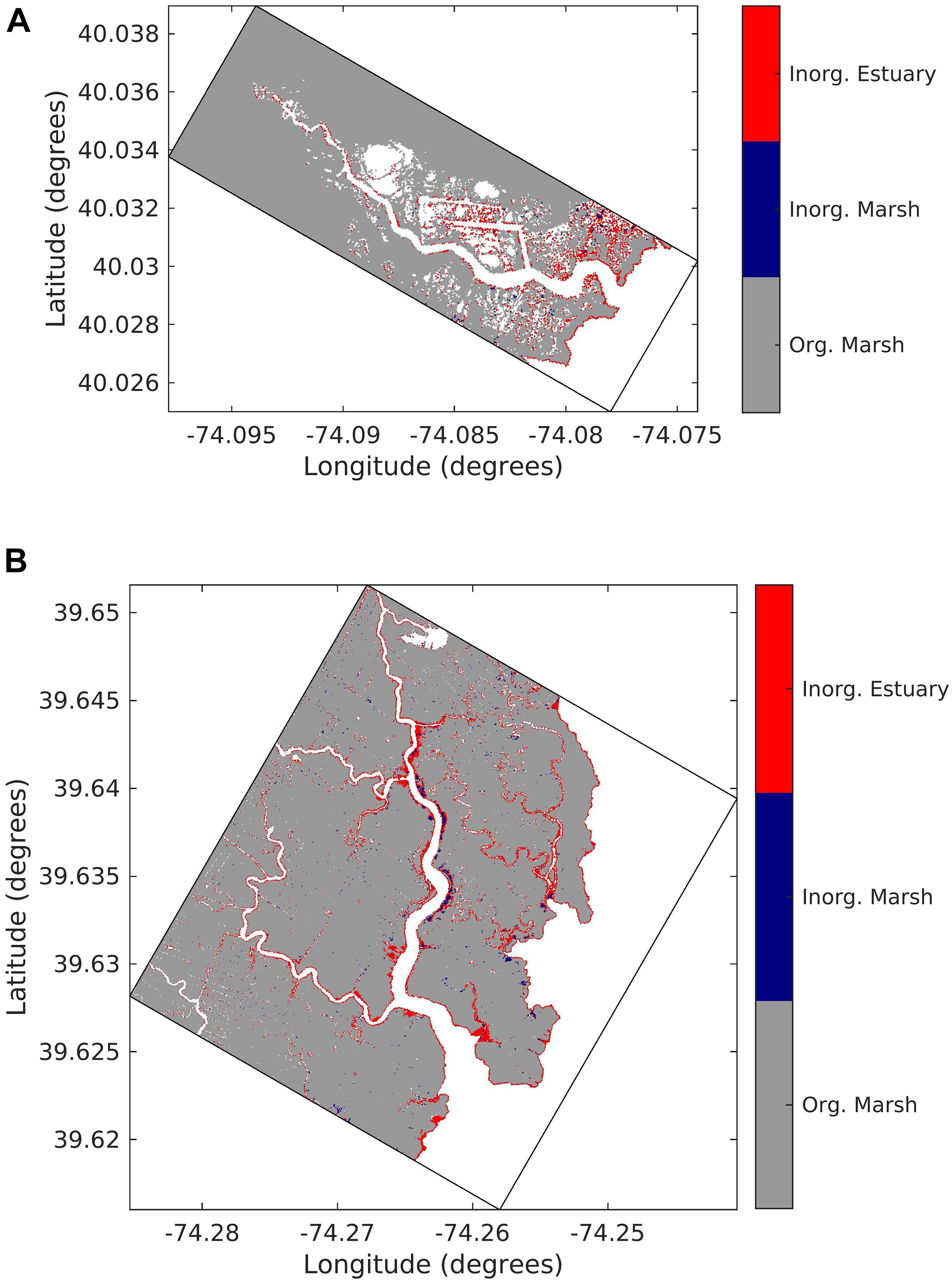
Figure 13. Combined pattern of sediment deposition on marsh cells at the end of the simulation coded with different colors for dominant source of sediment (gray = organic marsh, blue = inorganic marsh, red = inorganic estuarine sediment) in (A) Reedy Creek domain and (B) Dinner Creek domain. Color coding corresponds to a particular source of sediment if its contribution exceeds 50% in that cell. For example, if a cell gets a deposition of organic marsh sediment greater than 50%, that cell is coded with a gray color.
Limitations of the Model
The current methodology has several limitations that are listed below:
(a) The lateral erosion at different sites can depend on the spatially varying shoreline characteristics including geological, biological, and morphological factors leading to various geomorphic features of the remaining marsh (Hall et al., 1986; Allen, 1989; Schwimmer, 2001). In the current implementation of LWT based erosion, the marsh erodibility coefficient (kmarsh), which accounts for geomorphic properties, is currently a fixed user input for the entire domain.
(b) The erosion of marsh cells to open water due to the action of lateral thrust is being computed by accounting for the bathymetric change in the vertical direction. While a lateral wave thrust (LWT) should result in a horizontal retreat, the model is not capable of dynamically changing the grid cell in the lateral direction.
(c) The current choices of modeling are optimized to model marsh dynamics for monthly to annual time scales due to the restrictions imposed by the ocean modeling time steps, which is on the order of seconds.
(d) The process of undercutting or ponding on marshes leading to internal collapse of marsh systems are not included.
(e) The marsh sediment exported from lateral retreat and accumulated through autochthonous growth is restricted to be present only on the top bed layer. The biomass production that leads to vertical growth of organic matter is only limited to one class of sediment and vegetation (i.e., interspecies competition and facilitation are not considered).
(f) We currently do not account for sediment compaction and the associated land subsidence.
Ongoing Model Implementation and Its Potential Applications
Beyond the implementation presented in this article, ongoing work has included two additional functions that are available for a variety of applications. First, the growth of marsh vegetation based on peak biomass using relationships mentioned in D’Alpaos et al. (2006) to calculate the change in stem density, stem length, and diameter based on peak biomass, implementing the feedbacks between growth of biomass and marsh vegetation properties. A second functionality involves the conversion of non-marsh cells (open water cells) into marsh cells, thereby allowing for modeling of marsh lateral expansion over tidal flat areas and allowing marsh vegetation cover to increase in an area. The modification of marsh vegetation properties based on biomass and creation of marsh cells could be used to explore the role of vegetation properties in altering marsh dynamics or studying the relationships between sediment supply and marsh coverage. Using these two functionalities along with morphological acceleration, an ongoing model application involves the study of long-term marsh formation under varying conditions of RSLR and sediment supply.
Conclusion and Future Work
In this work, the COAWST (Coupled Ocean-Atmosphere-Wave-Sediment Transport) modeling framework was extended to add two key marsh processes that affect marshes, erosion due to lateral wave thrust (LWT) and vertical accretion due to biomass productivity. Verification of the LWT and retreat formulations was performed on idealized systems prior to application to two creek systems in Barnegat Bay. The modeling framework based on Tonelli et al. (2010) provides a maximum LWT when the water level is equal to the marsh scarp height with LWT decreasing as the water level exceeds the marsh scarp height. A high-resolution idealized simulation demonstrates how application of LWT reproduces key features of marsh edge erosion illustrating the model’s ability to account for LWT-based marsh erosion and causing a change in bed thickness in the marsh and adjacent non-marsh cell. The changes in bed thickness leads to an evolution of bathymetry creating a mudflat seaward of the marsh complex that subsequently alters wave energy and produces dynamic variation of wave thrust further affecting the dynamic evolution of marsh edge. The = functioning of combined processes of LWT and vertical growth due to biomass production on marsh complexes is demonstrated by modeling two creek systems in Barnegat Bay. The pattern of sediment deposition on the two creeks illustrates the ability of the model to account for autochthonous and allochthonous growth of marsh systems. Between the creeks, a larger region of inorganic deposition occurs at the Dinner Creek site compared to the Reedy creek site because of the larger tidal range.
In the future, the current framework can be extended to further the understanding of sediment dynamics during restoration efforts on marsh complexes. Future work could include the study of the sensitivity of marsh dynamics to varying tidal ranges, wave conditions, marsh vegetation, and sediment properties. In future, researchers could compare the marsh shoreline erosion, delivery and accretion rates with the field data that could help in understanding and improving of the current parameterizations. Future modeling efforts can also study sea level rise scenarios that cause larger wave thrust on marsh edges by deepening of estuaries as hypothesized by Finkelsten and Hardaway (1988) and predicted through a model by Schwimmer and Pizzuto (2000) and Mariotti and Fagherazzi (2013b). Application of this modeling framework can be extended to study the efficacy of living shorelines in the form of coral reefs, or seagrass beds that can act as a natural buffer to the lateral retreat of marshes (Piazza et al., 2005; Gittman et al., 2016).
Data Availability Statement
The model data were released as per the USGS model data release policy, and separate digital object identifiers were created as part of the release (https://www.usgs.gov/products/data-and-tools/data-management/data-release, last accessed: September 09, 2021). The model output can be accessed through ScienceBase entries for the idealized domains and Barnegat Bay creek simulations, respectively, as: (Kalra et al., 2021a, https://doi.org/10.5066/P94HYOGQ and Kalra et al., 2021b, https://doi.org/10.5066/P9QO091Z).
Author Contributions
TK implemented the marsh dynamics model in the COAWST framework. At various stages of the project, NG, AA, JC, and JM, helped in the algorithmic development of the marsh dynamics model. TK, AA, and NG helped in the analysis of the results. ZD provided guidance with the BB model along with bathymetric and marsh coverage data for the creek simulations. All authors contributed toward writing and editing of the manuscript.
Funding
This work was supported by USGS Coastal and Marine Hazards and Resources Program.
Author Disclaimer
Any use of trade, firm, or product names is for descriptive purposes only and does not imply endorsement by the United States Government.
Conflict of Interest
The authors declare that the research was conducted in the absence of any commercial or financial relationships that could be construed as a potential conflict of interest.
Publisher’s Note
All claims expressed in this article are solely those of the authors and do not necessarily represent those of their affiliated organizations, or those of the publisher, the editors and the reviewers. Any product that may be evaluated in this article, or claim that may be made by its manufacturer, is not guaranteed or endorsed by the publisher.
Acknowledgments
We thank Kathryn Smith at the United States Geological Survey (USGS) St. Petersburg Coastal and Marine Science Center for reviewing this manuscript. We also thank John Warner at the USGS Woods Hole Coastal and Marine Science Center for his insightful suggestions to develop the modeling framework through the length of the project.
Supplementary Material
The Supplementary Material for this article can be found online at: https://www.frontiersin.org/articles/10.3389/fmars.2021.740921/full#supplementary-material
References
Alizad, K., Scott, C., Hagen, S. C., Morris, J. T., Bacopoulos, P., Bilskie, M. V., et al. (2016). A coupled, two-dimensional hydrodynamic-marsh model with biological feedback. Ecol. Modell. 327, 29–43. doi: 10.1016/j.ecolmodel.2016.01.013
Allen, J. R. L. (1989). Evolution of salt-marsh cliffs in muddy and sandy systems: a qualitative comparison of British west-coast estuaries. Earth Surf. Process. Landf. 14, 85–92. doi: 10.1002/esp.3290140108
Barbier, E. B., Georgiou, I. Y., Enchelmeyer, B., and Reed, D. J. (2013). The value of wetlands in protecting southeast Louisiana from hurricane storm surges. PLoS One 8:e58715. doi: 10.1371/journal.pone.0058715
Bendoni, M., Francalanci, S., Cappietti, L., and Solari, L. (2014). On salt marshes retreat: experiments and modeling toppling failures induced by wind waves. J. Geophys. Res. Earth Surf. 119, 603–620. doi: 10.1002/2013JF003000
Bendoni, M., Georgiou, I. Y., and Novak, A. B. (2021). “Marsh edge erosion,” in Salt Marshes: Function, Dynamics, and Stresses, eds D. M. FitzGerald and Z. J. Hughes (Cambridge: Cambridge University Press), 388–422. doi: 10.1017/9781316888933.018
Bendoni, M., Mel, R., Solari, L., Lanzoni, S., Francalanci, S., and Oumeraci, H. (2016). Insights into lateral marsh retreat mechanism through localized field measurements. Water Resour. 52, 1446–1464. doi: 10.1002/2015WR017966
Beudin, A., Kalra, T. S., Ganju, N. K., and Warner, J. C. (2017). Development of a coupled wave-current-vegetation interaction. Comput. Geosci. 100, 76–86. doi: 10.1016/j.cageo.2016.12.010
Booij, N., Ris, R. C., and Holthuijsen, L. H. (1999). A third-generation wave model for coastal regions, Part I, model description and validation. J. Geophys. Res. C 4, 7649–7666. doi: 10.1029/98JC02622
Carniello, L., Defina, A., and D’Alpaos, L. (2009). Morphological evolution of the Venice lagoon: evidence from the past and trend for the future. J. Geophys. Res. 114, 148–227. doi: 10.1029/2008JF001157
Carr, J., Giulio, M., Sergio, F., McGlathery, K., and Patricia, W. (2018). Exploring the impacts of seagrass on coupled marsh-tidal flat morphodynamics. Front. Environ. Sci. 6:92.
Carr, J., Guntenspergen, G., and Kirwan, M. (2020). Modeling marsh-forest boundary transgression in response to storms and sea-level rise. Geophys. Res. Lett. 47:e2020GL088998. doi: 10.1029/2020GL088998
Chen, Q., and Zhao, H. (2011). Theoretical models for wave energy dissipation caused by vegetation. J. Eng. Mech. 138, 221–229. doi: 10.1061/(ASCE)EM.1943-7889.0000318
Chen, S., Torres, R., and Goñi, M. A. (2016). The role of salt marsh structure in the distribution of surface sedimentary organic matter. Estuar. Coast. 39, 108–122. doi: 10.1007/s12237-015-9957-z
Cheong, S. M., Silliman, B., Wong, P. P., van Wesenbeeck, B., Kim, C. K., and Guannel, G. (2013). Coastal adaptation with ecological engineering. Nat. Clim. Chang. 9, 787–791. doi: 10.1038/nclimate1854
Coleman, D. J., Ganju, N. K., and Kirwan, M. L. (2020). Sediment delivery to a tidal marsh platform is minimized by source decoupling and flux convergence. J. Geophys. Res. 125:e2020JF005558. doi: 10.1029/2020JF005558
D’Alpaos, A. (2011). The mutual influence of biotic and abiotic components on the long-term ecomorphodynamic evolution of salt-marsh ecosystems. Geomorphology 126, 269–278. doi: 10.1016/j.geomorph.2010.04.027
D’Alpaos, A., Lanzoni, S., Marani, M., and Rinaldo, A. (2007). Landscape evolution in tidal embayments: modeling the interplay of erosion, sedimentation, and vegetation dynamics. J. Geophys. Res. 112:F01008. doi: 10.1029/2006JF000537
D’Alpaos, A., Lanzoni, S., Mudd, S. M., and Fagherazzi, S. (2006). Modeling the influence of hydroperiod and vegetation on the cross-sectional formation of tidal channels. Estuar. Coast. Shelf Sci. 69, 311–324. doi: 10.1016/j.ecss.2006.05.002
Defne, Z., and Ganju, N. K. (2016). Conceptual salt marsh units for wetland synthesis: Edwin B. Forsythe National Wildlife Refuge. New Jersey, NJ: U.S. Geological Survey Data Release, doi: 10.5066/F7QV3JPG
Defne, Z., Ganju, N. K., and Moriarty, J. M. (2019). Hydrodynamic and morphologic response of a back barrier estuary to an extratropical storm. J. Geophys. Res. Oceans 124, 7700–7717. doi: 10.1029/2019JC015238
Department of the Army, Waterways Experiment Station, Corps of Engineers (1984). Shore Protection Manual, 4th Edn, Vol. 1. Washington, DC: Coastal Engineering Research Center, 532.
Dijkema, K. S. (1987). “Changes in salt-marsh area in the Netherlands Wadden Sea after 1600,” in Vegetation Between Land and Sea. Geobotany, Vol. 11, eds A. H. L. Huiskes, C. W. P. M. Blom, and J. Rozema (Dordrecht: Springer), doi: 10.1007/978-94-009-4065-9_4
Donatelli, C., Ganju, N. K., Fagherazzi, S., and Leonardi, N. (2018). Seagrass impact on sediment exchange between tidal flats and salt marsh, and the sediment budget of shallow bays. Geophys. Res. Lett. 45, 4933–4943. doi: 10.1029/2018GL078056
Evans, B. R., Möller, I., Spencer, T., and Smith, G. (2019). Dynamics of salt marsh margins are related to their three-dimensional functional form. Earth Surf. Process. Landf. 44, 1816–1827. doi: 10.1002/esp.4614
Fagherazzi, S. (2014). Coastal processes: storm-proofing with marshes. Nat. Geosci. 7, 701–702. doi: 10.1038/ngeo2262
Fagherazzi, S., Kirwan, M. L., Mudd, S. M., Guntenspergen, G. R., Temmerman, S., D’Alpaos, A., et al. (2012). Numerical models of salt marsh evolution: ecological and climatic factors. Rev. Geophys. 50:RG1002.
Finkelsten, K., and Hardaway, C. S. (1988). Late Holocene sedimentation and erosion of estuarine fringing marshes, York River, Virginia. J. Coast. Res. 4, 447–456.
Finotello, A., Marani, M., Carniello, L., Pivato, M., Roner, M., Tommasini, L., et al. (2020). Control of wind-wave power on morphological shape of salt marsh margins. Water Sci. Eng. 13, 45–56. doi: 10.1016/j.wse.2020.03.006
FitzGerald, D. M., Hein, C. J., Hughes, Z., Kulp, M., Georgiou, I., and Miner, M. (2018). “Runaway barrier island transgression concept: global case studies,” in Barrier Dynamics and Response to Changing Climate, eds L. Moore and A. Murray (Cham: Springer), 3–56. doi: 10.1007/978-3-319-68086-61
Francalanci, S., Paris, E., and Solari, L. (2013). A combined field sampling-modeling approach for computing sediment transport during flash floods in a gravel-bed stream. Water Resour. Res. 49, 6642–6655. doi: 10.1002/wrcr.20544
French, J. R. (1993). Numerical simulation of vertical marsh growth and adjustment to accelerated sea-level rise, North Norfolk, UK. Earth Surf. Process. Landf. 18, 63–81. doi: 10.1002/esp.3290180105
Ganju, N. K. (2019). Marshes are the new beaches: integrating sediment transport into restoration planning. Estuar. Coasts 42, 917–926. doi: 10.1007/s12237-019-00531-3
Ganju, N. K., Defne, Z., Kirwan, M. L., Fagherazzi, S., D’Alpaos, A., and Carniello, L. (2017). Spatially integrative metrics reveal hidden vulnerability of microtidal salt marshes. Nat. Commun. 8:14156. doi: 10.1038/ncomms14156
Ganju, N. K., Miselis, J. L., and Aretxabaleta, A. L. (2014). Physical and biogeochemical controls on light attenuation in a eutrophic, back-barrier estuary. Biogeosciences 11, 7193–7205. doi: 10.5194/bg-11-7193
Ganju, N. K., and Sherwood, C. R. (2010). Effect of roughness formulation onthe performance of a coupled wave, hydrodynamic, and sediment transport model. Ocean Modell. 33, 299–313. doi: 10.1016/j.ocemod.2010.03.003
Gittman, R. K., Peterson, C. H., Currin, C. A., Fodrie, F. J., Piehler, M. F., and Bruno, J. F. (2016). Living shorelines can enhance the nursery role of threatened estuary habitats. Ecol. Applic. 26, 249–263. doi: 10.1890/14-0716
Haidvogel, D. B., Arango, H. G., Budgell, W. P., Cornuelle, B. D., Curchitser, E., Di Lorenzo, E., et al. (2008). Ocean forecasting in terrain-following coordinates: formulation and skill assessment of the regional ocean modeling system. J. Comput. Phys. 227, 3595–3624. doi: 10.1016/j.jcp.2007.06.016
Hall, S. L., Wilder, W. R., and Fisher, F. M. (1986). An analysis of shoreline erosion along the Northern Coast of East Galveston Bay, Texas. J. Coast. Res. 2, 173–179.
Hopkinson, C. S., Morris, J. T., Fagherazzi, S., Wollheim, W. M., and Raymond, P. A. (2018). Lateral marsh edge erosion as a source of sediments for vertical marsh accretion. J. Geophys. Res. Biogeosciences 123, 2444–2465. doi: 10.1029/2017JG004358
Houttuijn Bloemendaal, L. J., FitzGerald, D. M., Hughes, Z. J., Novak, A. B., and Phippen, P. (2021). What controls marsh edge erosion? Geomorphology 386:107745. doi: 10.1016/j.geomorph.2021.107745
Kalra, T. S., Ganju, N. K., and Aretxabaleta, A. L. (2021a). Idealized Numerical Model for Marsh Lateral Wave Thrust and Retreat: U.S. Geological Survey Data Release. Reston, VA: U.S. Geological Survey, doi: 10.5066/P94HYOGQ
Kalra, T. S., Ganju, N. K., Defne, Z. D., and Aretxabaleta, A. L. (2021b). Numerical Model of Numerical Model of Barnegat Bay Creeks (Reedy and Dinner) to Demonstrate Marsh Dynamics Model: U.S. Geological Survey Data Release. Reston, VA: U.S. Geological Survey, doi: 10.5066/P9QO091Z
Kirwan, M. L., and Guntenspergen, G. R. (2010). Influence of tidal range on the stability of coastal marshland. J. Geophys. Res. 115:F02009. doi: 10.1029/2009JF001400
Kirwan, M. L., and Murray, A. B. (2007). A coupled geomorphic and ecological model of tidal marsh evolution. Proc. Natl. Acad. Sci. U.S.A. 104, 6118–6122.
Kirwan, M. L., and Temmerman, S. (2009). Coastal marsh response to historical and future sea-level acceleration. Q. Sci. Rev. 28, 1801–1808. doi: 10.1016/j.quascirev.2009.02.022
Kirwan, M. L., Walters, D. C., Reay, W. G., and Carr, J. A. (2016). Sea level driven marsh expansion in a coupled model of marsh erosion and migration. Geophys. Res. Lett. 43, 4366–4373. doi: 10.1002/2016GL068507
Kolker, A. S., Goodbred, S. L. Jr., Hameed, S., and Cochran, J. K. (2009). High-resolution records of the response of coastal wetland systems to long-term and short-term sea-level variability. Estuar. Coast. Shelf Sci. 84, 493–508. doi: 10.1016/j.ecss.2009.06.030
Lacy, J. R., Foster-Martinez, M. R., Allen, R. M., Ferner, M. C., and Callaway, J. C. (2020). Seasonal variation in sediment delivery across the bay-marsh interface of an estuarine salt marsh. J. Geophys. Res. Oceans 125:e2019JC015268. doi: 10.1029/2019JC015268
Le Hir, P., Monbet, Y., and Orvain, F. (2007). Sediment erodability in sediment transport modelling: can we account for biota effects? Cont. Shelf Res. 27, 1116–1142. doi: 10.1016/j.csr.2005.11.016
Leonardi, N., Defne, Z., Ganju, N. K., and Fagherazzi, S. (2016a). Salt marsh erosion rates and boundary features in a shallow Bay. J. Geophys. Res. Earth Surf. 121, 1861–1875. doi: 10.1002/2016JF003975
Leonardi, N., and Fagherazzi, S. (2014). How waves shape salt marshes. Geology 42, 887–890. doi: 10.1130/G35751.1
Leonardi, N., and Fagherazzi, S. (2015). Effect of local variability in erosional resistance affects large scale morphodynamic response of salt marshes to wind waves resistance affects large scale morphodynamic. Geophys. Res. Lett. 2015, 5872–5879. doi: 10.1002/2015GL064730
Leonardi, N., Ganju, N. K., and Fagherazzi, S. (2016b). A linear relationship between wave power and erosion determines salt-marsh resilience to violent storms and hurricanes. Proc. Natl. Acad. Sci. U.S.A. 113, 64–68. doi: 10.1073/pnas.1510095112
MARANI, M., D’Alpaos, A., Lanzoni, S., and Santalucia, M. (2011). Understanding and predicting wave erosion of marsh edges. Geophys. Res. Lett. 38:L21401. doi: 10.1029/2011GL048995
Mariotti, G. (2020). Beyond marsh drowning: the many faces of marsh loss (and gain). Adv. Water Resour. 144:103710. doi: 10.1016/j.advwatres.2020.103710
Mariotti, G., and Carr, J. (2014). Dual role of salt marsh retreat: long-term loss and short-term resilience. Water Resour. Res. 50, 2963–2974. doi: 10.1002/2013WR014676
Mariotti, G., and Fagherazzi, S. (2010). A numerical model for the coupled long-term evolution of salt marshes and tidal flats. J. Geophys. Res. Earth Surf. 115, 1–15. doi: 10.1029/2009JF001326
Mariotti, G., and Fagherazzi, S. (2013a). Critical width of tidal flats triggers marsh collapse in the absence of sea-level rise. Proc. Natl. Acad. Sci. U.S.A. 110, 5353–5356. doi: 10.1073/pnas.1219600110
Mariotti, G., and Fagherazzi, S. (2013b). A two-point dynamic model for the coupled evolution of channels and tidal flats. J. Geophys. Res. 118, 1387–1399. doi: 10.1002/jgrf.20070
Mariotti, G., Fagherazzi, S., Wiberg, P. L., McGlathery, K. J., Carniello, L., and Defina, A. (2010). Influence of storm surges and sea level on shallow tidal basin erosive processes. J. Geophys. Res. Oceans 115, 0148–0227. doi: 10.1029/2009JC005892
McKee, K. L., and Patrick, W. H. Jr. (1988). The relationship of smooth cordgrass (Spartina alterniflora) to tidal datums: a review. Estuaries 11, 143–151. doi: 10.2307/1351966
Möller, I. (2006). Quantifying saltmarsh vegetation and its effect on wave height dissipation: results from a UK East coast salt marsh. Estuar. Coast. Shelf Sci. 69, 337–351. doi: 10.1016/j.ecss.2006.05.003
Moller, I. (2014). Wave attenuation over coastal salt marshes under storm surge conditions. Nat. Geosci. 7, 727–731. doi: 10.1038/ngeo2251
Möller, I., Spencer, T., French, J. R., Leggett, D. J., and Dixon, M. (1999). Wave transformation over salt marshes: a field and numerical modelling study from North Norfolk, England. Estuar. Coast. Shelf Sci. 49, 411–426. doi: 10.1006/ecss.1999.0509
Morris, J. T., Barber, D. C., Callaway, J. C., Chambers, R., Hagen, S. C., Hopkinson, C. S., et al. (2016). Contributions of organic and inorganic matter to sediment volume and accretion in tidal wetlands at steady state. Earths Future 4, 110–121. doi: 10.1002/2015EF000334
Morris, J. T., Sundareshwar, P. V., Nietch, C. T., Kjerfve, B., and Cahoon, D. R. (2002). Responses of coastal wetlands to rising sea level. Ecology 83, 2869–2877.
Mudd, S. M., D’Alpaos, A., and Morris, J. T. (2010). How does vegetation affect sedimentation on tidal marshes? investigating particle capture and hydrodynamic controls on biologically mediated sedimentation. J. Geophys. Res. 115:F03029. doi: 10.1029/2009JF001566.NAM-12
Mudd, S. M., Howell, S. M., and Morris, J. T. (2009). Impact of dynamic feedbacks between sedimentation, sea-level rise, and biomass production on near-surface marsh stratigraphy and carbon accumulation. Estuar. Coast. Shelf Sci. 82, 377–389. doi: 10.1016/j.ecss.2009.01.028
NCEP NAM (2020). NAM-12 North America, NOAA Operational Model Archive and Distribution System. Available online at: https://nomads.ncep.noaa.gov
Neubauer, S. C. (2008). Contributions of mineral and organic components to tidal freshwater marsh accretion. Estuar. Coast. Shelf Sci. 78, 78–88. doi: 10.1016/j.ecss.2007.11.011
OCM Partners (2021). CoNED Topobathymetric Model for New Jersey and Delaware, 1880 to 2014 from 2010-06-15 to 2010-08-15. NOAA National Centers for Environmental Information. Available online at: https://www.fisheries.noaa.gov/inport/item/49467
Orson, R., Panageotou, W., and Leatherman, S. P. (1985). Response of tidal salt marshes of the U.S. Atlantic and Gulf Coasts to rising sea levels. J. Coast. Res. 1, 29–37. doi: 10.1086/716512
Piazza, B. P., Banks, P. D., and La Peyre, M. K. (2005). The potential for created oyster shell reefs as a sustainable shoreline protection strategy in Louisiana. Restor. Ecol. 13, 499–506. doi: 10.1111/j.1526-100X.2005.00062.x
Priestas, A. M., Mariotti, G., Leonardi, N., and Fagherazzi, S. (2015). Coupled wave energy and erosion dynamics along a salt marsh boundary, Hog Island Bay, Virginia, USA. J. Mar. Sci. Eng. 3, 1041–1065. doi: 10.3390/jmse3031041
Quirk, T. E. (2016). Impact of hurricane sandy on salt marshes of New Jersey. Estuar. Coast. Shelf Sci. 183, 235–248. doi: 10.1016/j.ecss.2016.09.006
Redfield, A. C. (1972). Development of a New England salt marsh. Ecol. Monogr. 42, 201–237. doi: 10.2307/1942263
Reed, D., Spencer, T., Murray, A., French, J., and Leonard, L. (1999). Marsh surface sediment deposition and the role of tidal creeks: implications for created and managed coastal marshes. J. Coast. Conserv. 5, 81–90. doi: 10.1007/bf02802742
Roner, M., D’Alpaos, A., Ghinassi, M., Marani, M., Silvestri, S., Franceschinis, E., et al. (2016). Spatial variation of salt-marsh organic and inorganic deposition and organic carbon accumulation: inferences from the Venice lagoon, Italy. Adv. Water Resour. 93(Pt B), 276–287. doi: 10.1016/j.advwatres.2015.11.011
Schwimmer, R. A. (2001). Rate and processes of marsh shoreline erosion in Rehoboth Bay, Delaware, USA. J. Coast. Res. 17, 672–683. doi: 10.2307/4300218
Schwimmer, R. A., and Pizzuto, J. E. (2000). A model for the evolution of marsh shorelines. J. Sediment. Res. 70:1026. doi: 10.1306/030400701026
Smith, K. E. L., Terrano, J. F., Khan, N. S., Smith, C. G., and Pitchford, J. L. (2021). Lateral shoreline erosion and shore-proximal sediment deposition on a coastal marsh from seasonal, storm and decadal measurements. Geomorphology 389:107829. doi: 10.1016/j.geomorph.2021.107829
Suttles, S. E., Ganju, N. K., Montgomery, E. T., Dickhudt, P. J., Borden, Jonathan, Brosnahan, S. M., et al. (2016). Summary of Oceanographic and Water–Quality Measurements in Barnegat Bay, New Jersey, 2014–15: U.S. Geological Survey Open-File Report 2016–1149. Roston, VA: U.S. Geological Survey, 22. doi: 10.3133/ofr20161149
Sutton-Grier, A. E., Wowk, K., and Bamford, H. (2015). Future of our coasts: the potential for natural and hybrid infrastructure to enhance the resilience of our coastal communities, economies and ecosystems. Environ. Sci. Policy 51, 137–148. doi: 10.1016/j.envsci.2015.04.006
Szpilka, C., Dresback, K., Kolar, R., Feyen, J., and Wang, J. (2016). Improvements for the western north atlantic, caribbean and gulf of mexico adcirc tidal database (EC2015). J. Mar. Sci. Eng. 4:72. doi: 10.3390/jmse4040072
Tambroni, N., and Seminara, G. (2006). Are inlets responsible for the morphological degradation of Venice Lagoon? J. Geophys. Res. 111:F03013. doi: 10.1029/2005JF000334
Temmerman, S., Bouma, T. J., Govers, G., Wang, Z. B., DeVries, M. B., and Herman, P. M. J. (2005). Impact of vegetation on flow routing and sedimentation patterns: three dimensional modeling for a tidal marsh. J. Geophys. Res. Earth Surf. 110:F04019. doi: 10.1029/2005JF000301
Temmerman, S., Govers, G., Meire, P., and Wartel, S. (2003). Modelling long-term tidal marsh growth under changing tidal conditions and suspended sediment concentrations, Scheldt Estuary, Belgium. Mar. Geol. 193, 151–169.
Temmerman, S., Meire, P., Bouma, T. J., Herman, P. M. J., Ysebaert, T., and De Vriend, H. J. (2013). Ecosystem-based coastal defence in the face of global change. Nature 504, 79–83. doi: 10.1038/nature12859
Tommasini, L., Carniello, L., Ghinassi, M., Roner, M., and D’Alpaos, A. (2019). Changes in the wind-wave field and related salt-marsh lateral erosion: inferences from the evolution of the Venice Lagoon in the last four centuries. Earth Surf. Process. Landfor. 44, 1633–1646. doi: 10.1002/esp.4599
Tonelli, M., Fagherazzi, S., and Petti, M. (2010). Modeling wave impact on salt marsh boundaries. J. Geophys. Res. 115:C09028. doi: 10.1029/2009JC006026
van de Koppel, J., van der Wal, D., Bakker, J. P., and Herman, P. M. (2005). Self-organization and vegetation collapse in salt marsh ecosystems. Am. Nat. 165, E1–E12. doi: 10.1086/426602
Warner, J. C., Armstrong, B., He, R., and Zambon, J. B. (2010). Development of a coupled ocean-atmosphere-wave-sediment transport (COAWST) modeling system. Ocean Modell. 35, 230–244. doi: 10.1016/j.ocemod.2010.07.010
Warner, J. C., Defne, Z., Haas, K., and Arango, H. G. (2013). A wetting and drying scheme for ROMS. Comput. Geosci. 58, 54–61. doi: 10.1016/j.cageo.2013.05.004
Warner, J. C., Sherwood, C. R., Arango, H. G., and Signell, R. P. (2005). Performance of four turbulence closure models implemented using a generic length scale method. Ocean Modell. 8, 81–113. doi: 10.1016/j.ocemod.2003.12.003
Warner, J. C., Sherwood, C. R., Signell, R. P., Harris, C. K., and Arango, H. G. (2008). Development of a three-dimensional, regional, coupled wave, current, and sediment-transport model. Comput. Geosci. 34, 1284–1306. doi: 10.1016/j.cageo.2008.02.012
Keywords: marsh morphology, sediment transport, numerical model, COAWST model, marsh accretion
Citation: Kalra TS, Ganju NK, Aretxabaleta AL, Carr JA, Defne Z and Moriarty JM (2021) Modeling Marsh Dynamics Using a 3-D Coupled Wave-Flow-Sediment Model. Front. Mar. Sci. 8:740921. doi: 10.3389/fmars.2021.740921
Received: 13 July 2021; Accepted: 06 October 2021;
Published: 02 November 2021.
Edited by:
Zhi-jun Dai, East China Normal University, ChinaReviewed by:
Alvise Finotello, Ca’ Foscari University of Venice, ItalyPeng Yao, Hohai University, China
Copyright © 2021 Kalra, Ganju, Aretxabaleta, Carr, Defne and Moriarty. This is an open-access article distributed under the terms of the Creative Commons Attribution License (CC BY). The use, distribution or reproduction in other forums is permitted, provided the original author(s) and the copyright owner(s) are credited and that the original publication in this journal is cited, in accordance with accepted academic practice. No use, distribution or reproduction is permitted which does not comply with these terms.
*Correspondence: Tarandeep S. Kalra, dGthbHJhQGNvbnRyYWN0b3IudXNncy5nb3Y=