Red Tide Events and Seasonal Variations in the Partial Pressure of CO2 and Related Parameters in Shellfish-Farming Bays, Southeastern Coast of Korea

Mixed results have been reported on the evaluation of the coastal carbon cycle and its contribution to the global carbon cycle, mainly due to the shortage of observational data and the considerable spatiotemporal variability arising from complex biogeochemical factors. In this study, the partial pressure of carbon dioxide (pCO₂) and related environmental factors were measured in the Jinhae–Geoje–Tongyeong bay region of the southeastern Korean Peninsula in February 2014, August 2014, April 2015, and October 2015. The mean pCO₂ of surface seawater ranged from 215 to 471 μatm and exhibited a high correlation with the surface seawater temperature when data for August were excluded (R² = 0.69), indicating that the seasonal variation in CO₂ could be largely attributed to the variation in seawater temperature. However, a severe red tide event occurred in August 2014, when the lowest pCO₂ value was observed despite a relatively high seawater temperature. It is considered that the active biological production of phytoplankton related to red tides counteracted the summer increase in pCO₂. Based on the correlation between pCO₂ and temperature, the estimated decrease in pCO₂ caused by non-thermal factors was approximately 200 μatm. During the entire study period, the air–sea CO₂ flux ranged from −14.2 to 3.7 mmol m^–2 d^–1, indicating that the study area served as an overall sink for atmospheric CO₂, and only functioned as a weak source during October. The mean annual CO₂ flux estimated from the correlation with temperature was −5.1 mmol m^–2 d^–1. However, because this estimate did not include reductions caused by sporadic events of biological production, such as red tides and phytoplankton blooms, the actual uptake flux is considered to be higher. The mean saturation state (Ω_Ar) value of carbonate aragonite was 2.61 for surface water and 2.04 for bottom water. However, the mean Ω_Ar of bottom water was <2 in August and October, and the Ω_Ar values measured at some of the bottom water stations in August were <1. Considering that the period from August to October corresponds to the reproduction and growth stages of shellfish, such low Ω_Ar values could be very damaging to shellfish production and the aquaculture industry.

Introduction

Climate change caused by the increase in greenhouse gases in Earth’s atmosphere not only raises the temperature of the ocean, but also causes ocean acidification and deoxygenation, which are global concerns (IPCC, 2014). Ocean acidification is a phenomenon in which the ocean absorbs approximately 25% of anthropogenic carbon dioxide (CO₂) and lowers the pH of the ocean through carbonate chemistry. Compared with pre-industrial times, the pH of the open ocean has already decreased by approximately 0.1 pH units (Bates et al., 2014; Le Quéré et al., 2018). Due to the effects of pH changes in the complex biogeochemical processes, limited water exchange, eutrophication, and bottom hypoxia, ocean acidification is promoted in coastal regions, where pH exhibits a considerable spatiotemporal variability (Wallace et al., 2014; Carstensen et al., 2018; Jiang et al., 2019). In some areas, the inter-daily pH variation can exceed 1 pH unit (Duarte et al., 2013). The decrease in seawater pH due to ocean acidification affects the physiological activity, growth, and survival of aquatic organisms, as well as the saturation state of carbonate minerals, which could have a devastating impact on shellfish and coral reefs (Hoegh-Guldberg et al., 2007; Kroeker et al., 2013; Waldbusser et al., 2013; Pilcher et al., 2019). Therefore, there is an urgent need to assess the status and mechanism of ocean acidification in coastal zones that are characterized by numerous marine organisms and active fishery activities (e.g., fishing grounds and aquaculture). Moreover, it is also necessary to predict the corresponding impact on the future fishery industry.

However, as described above, compared with the open ocean environment, carbon-related parameters exhibit considerable spatiotemporal variabilities in coastal regions due to complex causes, such as the nutrient loading and pollutant influx from land, active primary production and decomposition, and mixing with bottom water or sediment layers. Thus, an accurate assessment of the carbonate system in coastal environments is challenging, and high-resolution spatiotemporal surveys and repeated surveys are necessary. However, few reports on coastal surveys are available, and there is no clear conclusion on the coastal contribution to the global ocean uptake of atmospheric CO₂ (Laruelle et al., 2014; Gruber, 2015). Based on observations from 165 estuaries and 87 continental shelves, Chen et al. (2013) estimated that estuaries worldwide emit 0.1 Pg C y^–1 into the atmosphere, while continental shelves absorb 0.4 Pg C y^–1 from the atmosphere. In addition, the authors found a considerable variation in the air–sea exchange of CO₂ with both season and latitude, and thus on the whole, there was more uptake from atmosphere in spring and winter than in summer and autumn (Chen et al., 2013). Laruelle et al. (2017) classified ten biogeochemical provinces controlled by latitudinal gradients and the distance from the coast and evaluated high-resolution monthly climate data of the partial pressure of CO₂ (pCO₂) for coastal oceans. For example, the pCO₂ values at coastal zones with a temperate climate in the Northern Hemisphere ranged from 325 to 370 μatm, and particularly in the case of western Pacific shelves in the temperate zone, the seasonal pCO₂ amplitudes were found to exceed 50 μatm. Roobaert et al. (2019) reported that the main factor influencing the air–sea exchange of CO₂ was the difference between the pCO₂ values of air and seawater (ΔpCO₂) in the region of 10–40° N, which has a typical seasonal cycle. The East China Sea and Kuroshio waters, which form part of the western boundary currents (WBC), were found to uptake 0.59 mol C m^–2 y^–1, whereas the East/Japan Sea (i.e., a marginal sea) was estimated to uptake 1.44 mol C m^–2 y^–1 (Roobaert et al., 2019).

Although there have been several attempts to evaluate or numerically model the distribution or uptake of CO₂ in coastal and marginal regions based on existing data, insufficient observation data and large spatiotemporal variabilities make accurate evaluation difficult (Gruber, 2015). Therefore, investigating the distribution characteristics of carbonate parameters and the corresponding influencing factors through intensive surveys is key for improving evaluations.

There have also been several studies conducted related to the ocean carbon cycle and acidification for coastal and marginal seas around the Korean Peninsula. From 14 observations collected during 1995-2009 in the Ulleung Basin, the southwestern part of the East/Japan Sea absorbed 0.95 ± 0.53 mol C m^–2 y^–1 in 1995 and 0.81 ± 0.49 mol C m^–2 y^–1 in 2004, showing that the increase rate of fCO₂ and the acidification trend for the surface water were 2.7 ± 1.1 μatm y^–1 and −0.03 ± 0.02 pH units decade^–1, respectively (Kim et al., 2014). Kim et al. (2018) also discussed aragonite saturation in the two coastal regions of South Korea. In summer, the surface Ω_arag values at the Busan coast under the influence of the Nakdong River were higher than those during other seasons; however, those at Gwangyang Bay near the Seomjin River showed very low Ω_arag (∼0.77) in the surface layer. The contradictory nature of these findings could have been caused by the different time-elapses after strong river discharge events in each of these areas and by the differences of freshwater exchange with the open sea, suggesting that more field measurements are needed for understanding the coastal carbon cycles and impacts to fisheries in these areas (Kim et al., 2018).

This study obtained observations of marine environmental and carbonate factors in the Jinhae–Geoje-Tongyeong Bay region of the southeastern coast in Korea, examined their spatiotemporal variability, and evaluated the factors influencing surface pCO₂. Based on the characteristics of carbonate parameters in this region accounting for 80–90% of oyster and 70–85% of shellfish aquaculture production in Korea (Korean Statistical Information Service (KOSIS, 2021), this study could provide a reference basis in studying the impacts of environmental changes (e.g., increasing seawater temperatures and ocean acidification) on the aquaculture and fishery industries in these coastal waters.

Materials and Methods

Study Area

The southeastern coast of Korea, which includes the study area, is a semi-enclosed bay of the Rias coast, where limited water exchange occurs with the open sea. The area is characterized by fishing and aquaculture activities owing to the abundant food and nutrients within the inflowing freshwater from adjacent land. The study area consists of Jinhae Bay (JB), Geoje-Hansan Bay (GHB), and Tongyeong-Goseong Bay (TGB) of Gyeongsangnam-do Province (Figure 1). Approximately 2.5–3.0 × 10⁵ tons of oysters, blue mussels, and scallops are produced annually through aquaculture in the entire study area, which accounts for >80% of the production of shellfish farming in Korea.

FIGURE 1

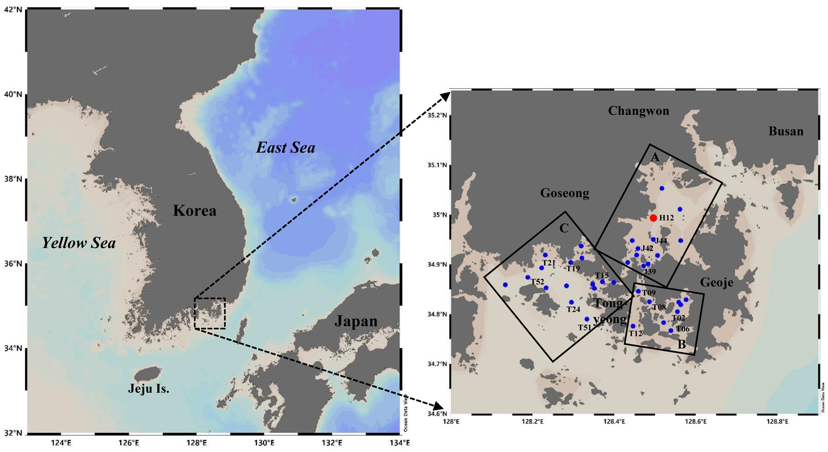
Figure 1. Study site showing the three areas [A: Jinhae Bay (JB), B: Geoje-Hansan Bay (GHB), C: Tongyeong- Goseong Bay (TGB)] and discrete stations (blue circles) with one hypoxia monitoring station HI2 (red circle).

However, since the 1970s, industrialization has led to coastal development and construction activities along with the introduction of a variety of organic pollutants; hence, the area has experienced frequent red tides (i.e., harmful algal blooms) and hypoxia as well as the mass mortality of aquaculture species (Lee et al., 2018). Although water quality has improved since the late 1990s due to enforced onshore sewage treatment and increased environmental awareness, the area has still been affected by seasonal red tide events and hypoxia in its bottom water (Kwon et al., 2014; Lee et al., 2018; Lim et al., 2020).

Jinhae Bay is a semi-enclosed bay (mean depth of ∼20 m) with a dominantly semidiurnal tide. The majority of seawater exchange (80–90%) occurs through the Gadeok Channel in the eastern part of the bay, and the remaining seawater exchange occurs via the Gyeonnaeryang Channel in the southern part of the bay. Small inner bays such as Masan Bay, Jindong Bay, Danghangpo Bay, Dangdong Bay, Wonmun Bay, Gohyeon Bay, and Haengam Bay are distributed within JB. The semi-enclosed characteristics of JB, such as prolonged residence time, can lead to the accumulation of even small amounts of pollutants; hence, the area has been frequently affected by hypoxia, organic pollution, red tides, and mortality of marine organisms (Kwon et al., 2014; Lee et al., 2018). Consequently, some waters in the area were designated as special management marine areas in the 2000s, and a total pollution load management system was implemented for the chemical oxygen demand (COD), total nitrogen, and total phosphorus. As a result, the COD of bottom water and nutrient concentrations [dissolved inorganic nitrogen (DIN) and dissolved inorganic phosphorus (DIP)] of surface water and bottom water showed decreasing trends in most areas of JB (Kwon et al., 2014). Geoje-Hansan Bay is surrounded by four islands and is divided into the inner bay (Geoje Bay) and the water channel (Hansan Bay). The bay is semi-enclosed and is connected to the open sea in the southeast and to JB through a narrow channel in the northwest. An assessment of the ecological carrying capacity of the oyster farms in GHB showed that a reduction of 40–60% relative to the present status was an appropriate capacity of the farms (Cho et al., 2012). Tongyeong-Goseong Bay is mainly an open water area in comparison to JB and GHB. It borders the Korea Strait to the south and land to the northwest, and includes small bays such as Goseong Bay, Jaran Bay, and Bukshin Bay. In particular, the environmental parameters of the coastal waters of TGB exhibit large spatiotemporal variabilities due to the development of a coastal front where the river-dominated coastal water and Tsushima water of the open sea meet.

Underwater Real-Time Measurement of Surface Seawater

The research vessel Tamgu 17 (National Institute of Fisheries Science, or NIFS) was used to continuously measure the temperature, salinity, pCO₂, and pH of surface seawater in JB (area A), GHB (area B), and TGB (area C) in February 2014, August 2014, April 2015, and October 2015 (Figure 1). The surface seawater along the transects taken distally between stations to cover the whole area was pumped using a submersible pump (∼1 m depth) branched into two sides; one side was passed through a pH sensor (WTW pH3310, Xylem Analytics, Germany) and thermosalinograph (SBE45, Sea-Bird Electronics, United States) to measure pH and temperature/salinity, respectively, while the other side was supplied to a CO₂ measurement system. In accordance with one guide for ocean CO₂ measurements (Dickson et al., 2007), the seawater pCO₂ measurement system used a showerhead equilibrator to spray seawater particles, and the atmospheric CO₂ that was in equilibrium with the CO₂ in the air of the equilibrator was measured using a non-dispersive infrared analyzer (NDIR840, LiCor, United States). The continuous temperature and salinity measurements of surface seawater from the thermosalinograph were compared with those of a conductivity–temperature–depth (CTD) profiler (19plus, Sea-Bird Electronics, United States) (see the following section).

The CO₂ exchange fluxes across the sea-air interface were calculated from

$$\text{F}(\text{mmol}{\text{m}}^{-2}{\text{d}}^{-1})=k\times \mathrm{s}\times \mathrm{\Delta }p{\mathrm{CO}}_2(1)$$

where k is the gas transfer velocity (cm h^–1), s is the solubility of CO₂ gas in seawater (mol kg^–1 atm^–1) (Weiss, 1974), and ΔpCO₂ is the sea–air differences of CO₂ partial pressure. The parameterization implies that fluxes at the sea–air interface into the surface water (sinks) are negative and fluxes to the atmosphere (sources) are positive. We used the formula for k and the wind speed relationships from Wanninkhof (1992, 2014) to allow for comparison of our results with those of most other studies. This study used the mean monthly wind speed (2011–2015) of the marine meteorological observation buoy installed in the waters of Geoje Island by Korea Meteorological Administration (KMA), and the mean monthly air CO₂ concentration (2014–2015) of the Anmyeon greenhouse gas monitoring station, also operated by KMA (Korea Meteorological Administration, 2021).

To quantify the thermal and non-thermal effects on the surface pCO₂ distribution, the equations proposed by Takahashi et al. (1993, 2002) were used. Takahashi et al. (1993) experimentally determined the net effect of temperature on pCO₂ for isochemical seawater in surface water samples from the North Atlantic, and this value was used as a constant applied for most of seawater conditions (δlnpCO₂/δT = 0.0423°C^–1). For a quantitative evaluation of the temperature effect between the surveys, the CO₂ concentration due to the seasonal variation in temperature (excluding other factors) was calculated using Eq. 2 (Takahashi et al., 2002):

$$\begin{array}{c}(p{\text{CO}}_2\mathrm{at}{\text{T}}_{\text{obs}})=(\text{Mean}\text{annual}p{\text{CO}}_2)\times \hfill \\ \exp [0.0423(T_{\text{obs}}-T_{\text{mean}})].\hfill \end{array}(2)$$

In addition, if the pCO₂ concentration of each survey period is normalized to the mean temperature of the entire survey period, this represents the variation caused by non-thermal factors, which can be calculated as follows:

$$\begin{array}{c}(p{\text{CO}}_2\mathrm{at}{\text{T}}_{\text{mean}})={(p{\text{CO}}_2)}_{\text{obs}}\times \hfill \\ \exp [0.0423(T_{\text{mean}}-T_{\text{obs}})].\hfill \end{array}(3)$$

In this equation, for the mean annual pCO₂ and T_mean, the mean CO₂ concentration and mean seawater temperature of the entire survey period were used. For (pCO₂)_obs and T_obs, the mean CO₂ concentration and mean temperature of each survey period were used.

Station Surveys and Water Quality Analysis

To supplement the analysis of the results from the real-time continuous measurement system and to examine the environmental parameters in the water column, data from 25 to 28 stations were used for each survey (i.e., February 2014, August 2014, April 2015, and October 2015) (Figure 1). At each station, the temperature and salinity were measured from the surface to the bottom water using the CTD profiler. In addition, for the analysis of nutrients, dissolved oxygen (DO), chlorophyll-a, and dissolved inorganic carbon (DIC) of surface water (∼1 m depth) and bottom water (2–3 m upper depth from bottom layer), samples were collected with a Niskin water sampler, pre-treated according to the parameter, and stored for later analysis. The DO concentration was analyzed in situ by the Winkler method using a titrator (Dosimat 876 system, Metrohm, Switzerland) and pretreatment and analysis for chlorophyll-a was performed in accordance with the Korean standard method of examination for the marine environment (Ministry of Oceans and Fisheries (MOF, 2013). For the analysis of nutrients, an automatic analyzer (QuAAtro system with four channels, BranLuebbe, Germany) was used in the laboratory for samples previously filtered through GF/F filters before freezing/storage, and the analysis results were verified against relevant reference materials (reference materials for nutrients in seawater, KANSO CO. LTD., Japan). Dissolved inorganic carbon was analyzed using an AS-C3 instrument (Apollo SciTech, United States) and verified against the certified reference materials produced by Dr. A. Dickson’s laboratory at the Scripps Institute, United States. Total alkalinity (TA) and aragonite saturation state (Ω_Ar) were calculated from the values of DIC and pH using the CO2SYS program (Pierrot et al., 2006).

As a representative of national fisheries research institute, NIFS has conducted coastal environmental surveys specially focused on outbreaks of hypoxia and red-tide, as well as nation-wide regular monitoring around aquaculture areas, and archived all field data on the web-based data platform of Korea Oceanographic Data Center (Korea Oceanographic Data Center, 2021). In 2014, hypoxia developed initially on May 21st in JB and was monitored until 5th November with 11 total surveys during that period including surveys on August 5th and 28th. For outbreaks of algal blooms (Akashiwo sanguinea) on May 8th and of harmful algal blooms [Margalefidinium polykrikoides (a.k.a. Cochlodinium polykrikoides)] on July 31st, specially focused red-tide monitoring was also conducted at Tongyeong-Geoje Bay at an interval of 2–3 weeks from May through October. Further, baseline red-tide monitoring was conducted monthly from May to November at 26 stations covering the entire study area. From the data platform of KODC, we used the hypoxia and red-tide survey data to complement the environmental parameters and phytoplankton biomass information before and after the August 2014 survey, and also used the regular bimonthly monitoring data for aquaculture areas to calculate the monthly temperature change.

The maps reported in this study (Figure 1), as well as all charts depicting seawater temperature, salinity, pCO₂ and related parameters were created using Ocean Data View (Schlitzer, R., Ocean Data View, odv.awi.de, 2018) with weighted-average gridding and default options, including automatic scale lengths and color shading.

Results

Seasonal Variations in Surface pCO₂, pH, and Temperature

The continuous measurement data of temperature, salinity, pH, and pCO₂ in the surface seawater of JB (area A), GHB (area B), and TGB (area C) showed marked seasonal variabilities (Figures 2, 3). In February 2014, the mean (range) temperature and salinity were 8.9°C (6.6–12.4°C) and 33.59 (20.37–34.29), respectively, which were the lowest temperature and highest salinity values of the entire study period (Figures 2A,E). In August 2014, the mean temperature and salinity were 26.7°C (24.3–29.4°C) and 26.73 (12.47–31.84), respectively, which were the highest temperature and lowest salinity values of the entire study period (Figures 2C,G). In April 2015, the mean surface temperature and salinity were 15.7°C (14.4–17.9°C) and 32.25 (30.32–33.79), respectively, while they were 24.1°C (21.5–25.7°C) and 31.88 (31.27–32.91), respectively, in October 2015. The spatial variabilities of temperature and salinity in April and October were relatively small with more uniform distributions compared with those in February and August (Figure 2).

FIGURE 2

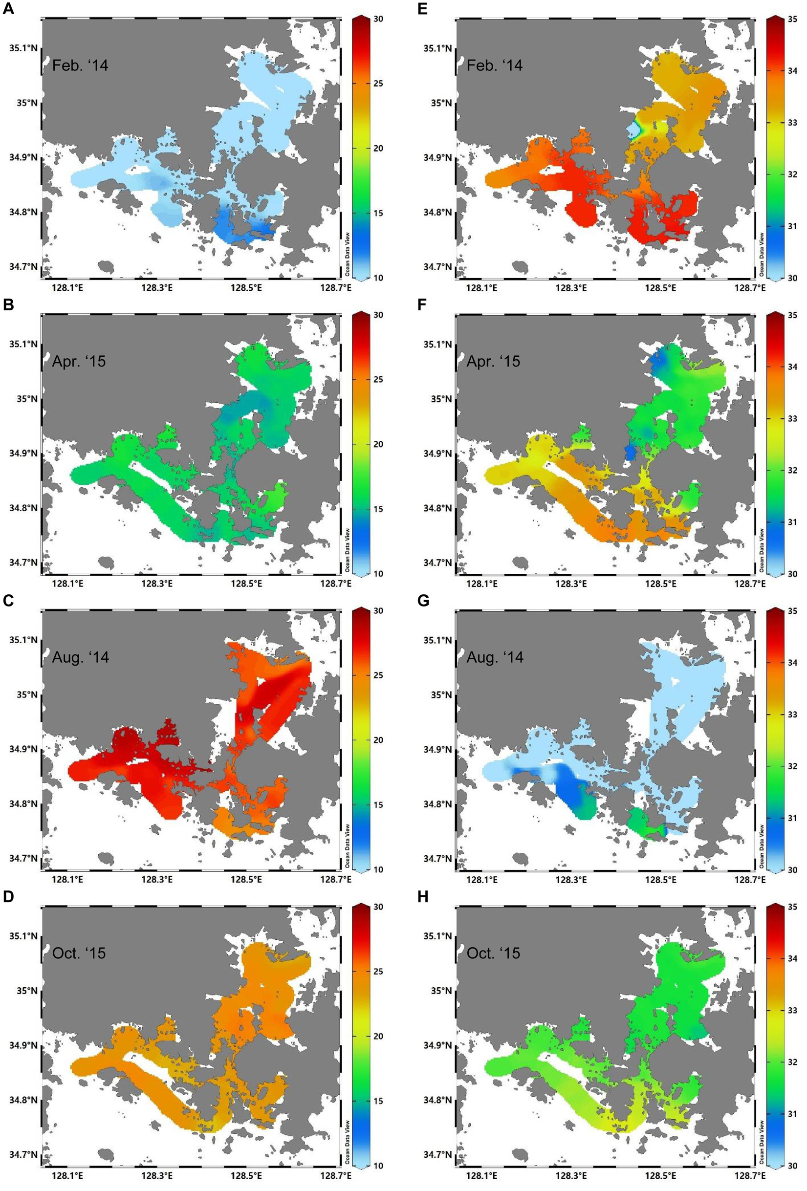
Figure 2. Distributions of sea surface temperature (°C) (A–D) and salinity (E–H) for each survey.

FIGURE 3

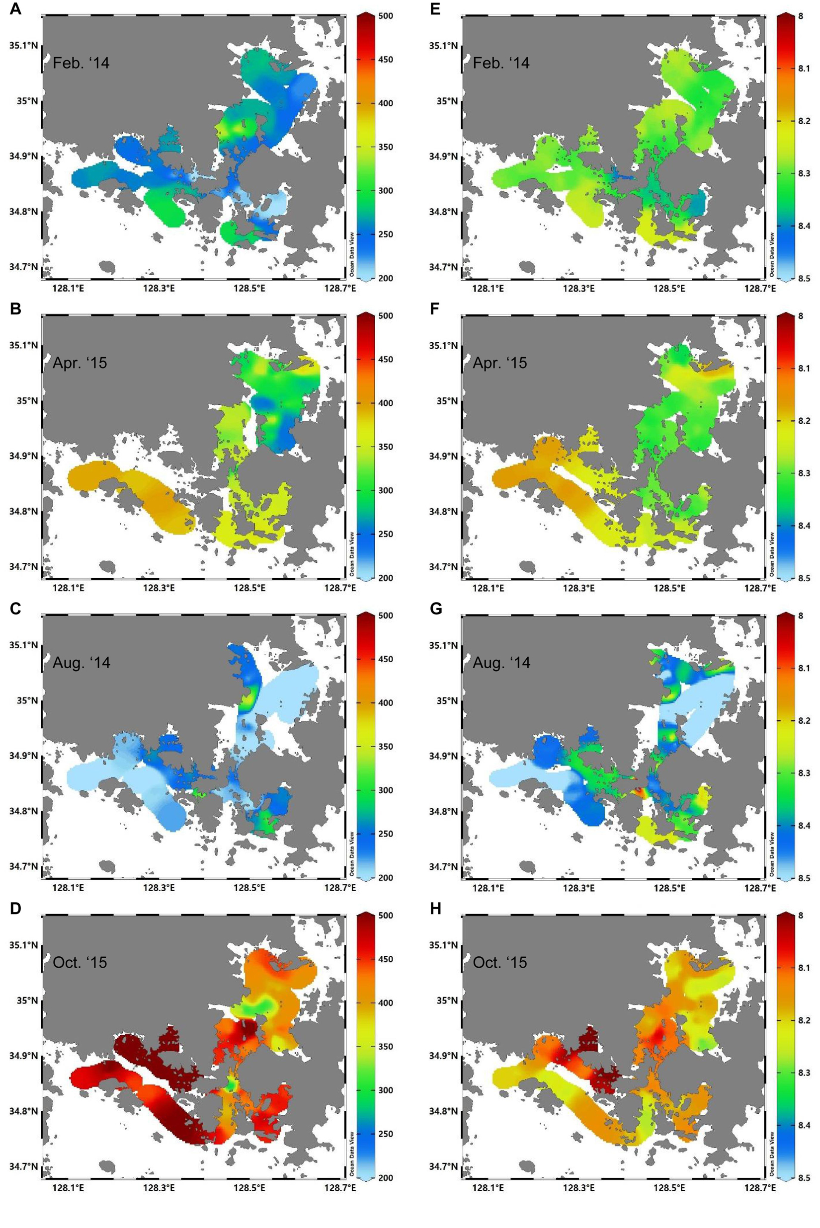
Figure 3. Distributions of sea surface pCO₂ (μatm) (A–D) and pH (E–H) for each survey. Reversed scale bar was applied for pH.

There were also differences in the spatial distributions of environmental factors between JB (area A), which is surrounded by land, TGB (area C), which is connected to the open sea, and GHB (area B), which is intermediate between the other two bays. In February 2014, the seawater temperature in the central part of area A (relatively close to the land) ranged from 7 to 9°C, whereas the temperature range in the open waters of area B and C was 9.5–12.0°C (Figure 2A). The mean salinity in area A (33.2) was also lower than those in area B and C (both ≥34), even after excluding some data for the southwest part of area A (salinity of <30) (Figure 2E). In August 2014, the highest mean temperature (>29°C) was observed in the small bays of area C (Goseong Bay and Jaran Bay). Similar to February, the mean salinity in the central part of area A was relatively low at 25.68 (16.46–31.41) in August, although this was slightly higher than that in area B (25.65), which was due to the low salinity in Geoje Bay (<20) (Figure 2G). In April and October 2015, the mean salinity value in the central part of JB (area A) was lower or similar to the values in areas B and C (open seawater), and the mean temperature in area A was slightly lower (by ∼0.4°C) than the values in areas B and C (Figures 2B,F). On the other hand, the temperature of the central part of area A was higher (0.5–0.8°C) than the values in areas of B and C in October (Figures 2D,H).

The distributions of pCO₂ and pH in surface water also exhibited distinct seasonal variations (Figure 3). In February 2014, when the water temperature was lowest, the mean pCO₂ was relatively low at 259 μatm, and thus the pH associated with carbonate chemistry was relatively high at 8.32. Conversely, in October 2015, when the mean pCO₂ was highest (471.4 μatm), the mean pH was lowest at 8.14. Despite the high temperature in August 2014, the pCO₂ value was the lowest of the entire survey period at just 215.1 μatm, while the mean pH was the highest (8.40). The mean pCO₂ in April 2015 was 346 μatm (pH of 8.26), which was lower than that in October 2015, but higher than the mean values in February and August 2014.

Examining the differences in the study area, in February, the mean difference in the pCO₂ values between areas A, B, and C was not large at <20 μatm; however, a low pCO₂ value was observed along the inner side of area B, which increased toward the outer water. This difference was also clearly observed in the pH distribution. In addition, the waters of areas A and C showed similar distributions in the pCO₂ values, although the pCO₂ value near Wonsan Bay in the central part of area A was abnormally high. In October, the highest mean pCO₂ value (536.8 μatm) was observed in area C, within which the highest individual values (up to 718 μatm) were measured in the small bays of Goseong Bay and Jaran Bay. A relatively high mean pCO₂ value of 439.5 μatm was observed in area B, which was characterized by a spatially uniform distribution, whereas a relatively low mean pCO₂ value was recorded in area A (416.5 μatm), with values of <400 μatm was observed in the central part of area A. The distribution of pH in surface seawater in October was similar to that of pCO₂, and was ≤8 in Goseong Bay and Jalan Bay in area C, while some measurements in area A were ≥8.3. In August, the lowest mean pCO₂ was in area A (176.3 μatm), followed by areas C and B, with slightly higher pCO₂ values in the mouth area and inner side of Geoje Bay in area B. The distribution of pH in surface seawater in August was also similar to that of pCO₂, with the highest mean pH in area A. In April, the lowest and highest mean pCO₂ values were measured in areas A and C, respectively, while the reverse was observed for pH.

Seasonal Variations in Dissolved Inorganic Carbon and Other Environmental Parameters at Stations

The distributions of temperature and salinity observed in the station surveys showed marked seasonal variabilities, similar to the real-time measurement results described in the previous section. The mean temperature and salinity of surface seawater in February was relatively low in area A, whereas it was higher in areas B and C (Table 1 and Figures 4A,E). As for surface water, the temperature and salinity values of bottom water were relatively low in area A (surrounded by land), whereas values were relatively high in areas B and C (linked to the open sea). The difference between the mean temperature of surface water and the mean temperature of bottom waters (based on all stations) was 0.35°C, while the difference in salinity was −0.05, indicating a well-mixed water column. In August, the temperature of surface seawater was highest in the small bays of areas A and C, and the salinity was <30 in the waters surrounded by small bays and land in areas B and C (Figures 4C,G). The temperature and salinity of bottom water showed similar trends to those of surface water. The lowest salinity (<11) was measured at a station close to the land in Geoje Bay. The largest mean differences in temperature and salinity between surface water and bottom water were in August (1.81°C and −1.85, respectively), indicating the formation of a stratified water column. In April, the highest temperatures of surface water were observed in the small bays of areas B and C, and the salinity values of areas B and C were ≥33 (difference in mean temperature and salinity between surface water and bottom water of 1.19°C and −0.35, respectively) (Figures 4B,F). Although most temperatures of bottom water were similar to those of surface water, and low temperatures were observed at a deep water level in the inner part of area A. In October, the temperatures of surface water and bottom water showed the most uniform distributions during the entire study period in all areas, and the salinity values of surface water and bottom water in area A were approximately 0.5 lower than those in areas B and C (difference in mean temperature and salinity between surface water and bottom water of 0.83°C and −0.43, respectively) (Figures 4D,H).

TABLE 1

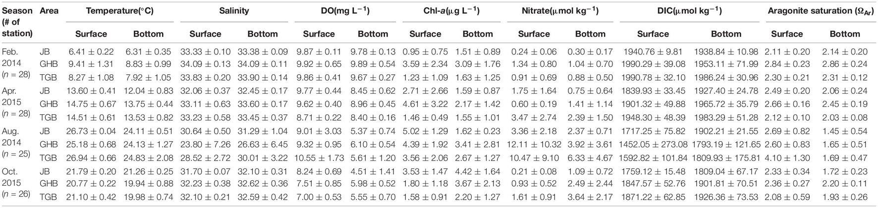
Table 1. Averages of temperature, salinity, DO, chlorophyll-a, nitrate, DIC, and aragonite saturation state in surface and bottom waters at three areas (JB: Jinhae Bay, GHB: Geoje-Hansan Bay, TGB: Tongyeong-Goseong Bay).

FIGURE 4

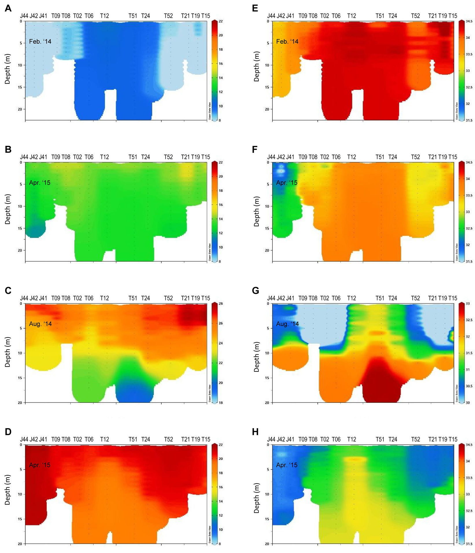
Figure 4. Vertical distributions of temperature (°C) (A–D) and salinity (E–H) for each surrvey. Different ranges of scale bar were applied for August 2014. Station numbers are shown on the upper x-axis and those locations are presented in Figure 1. Stations J44–J41 generally belong to JB, stations T09–T12 to GHR, and stations T51–T15 to TGB.

The highest mean DIC concentrations in surface water and bottom water were 1978.2 and 1966.1 μmol kg^–1, respectively, which were observed in February when the highest salinity values were recorded (Table 1 and Figures 5A,E). The lowest mean DIC concentrations in surface water and bottom water were 1562.1 and 1812.0 μmol kg^–1, respectively, which were observed in August (lowest salinity) (Figures 5C,G). In April, the mean DIC concentration of bottom water was 1958.9 μmol kg^–1, which was similar to that in February, while the mean DIC concentration of surface water was 1897.9 μmol kg^–1, which was lower than that in February (Figures 5B,F). In October, the mean DIC concentrations of surface water and bottom water were 1825.2 and 1878.3 μmol kg^–1, respectively (Figures 5D,H).

FIGURE 5

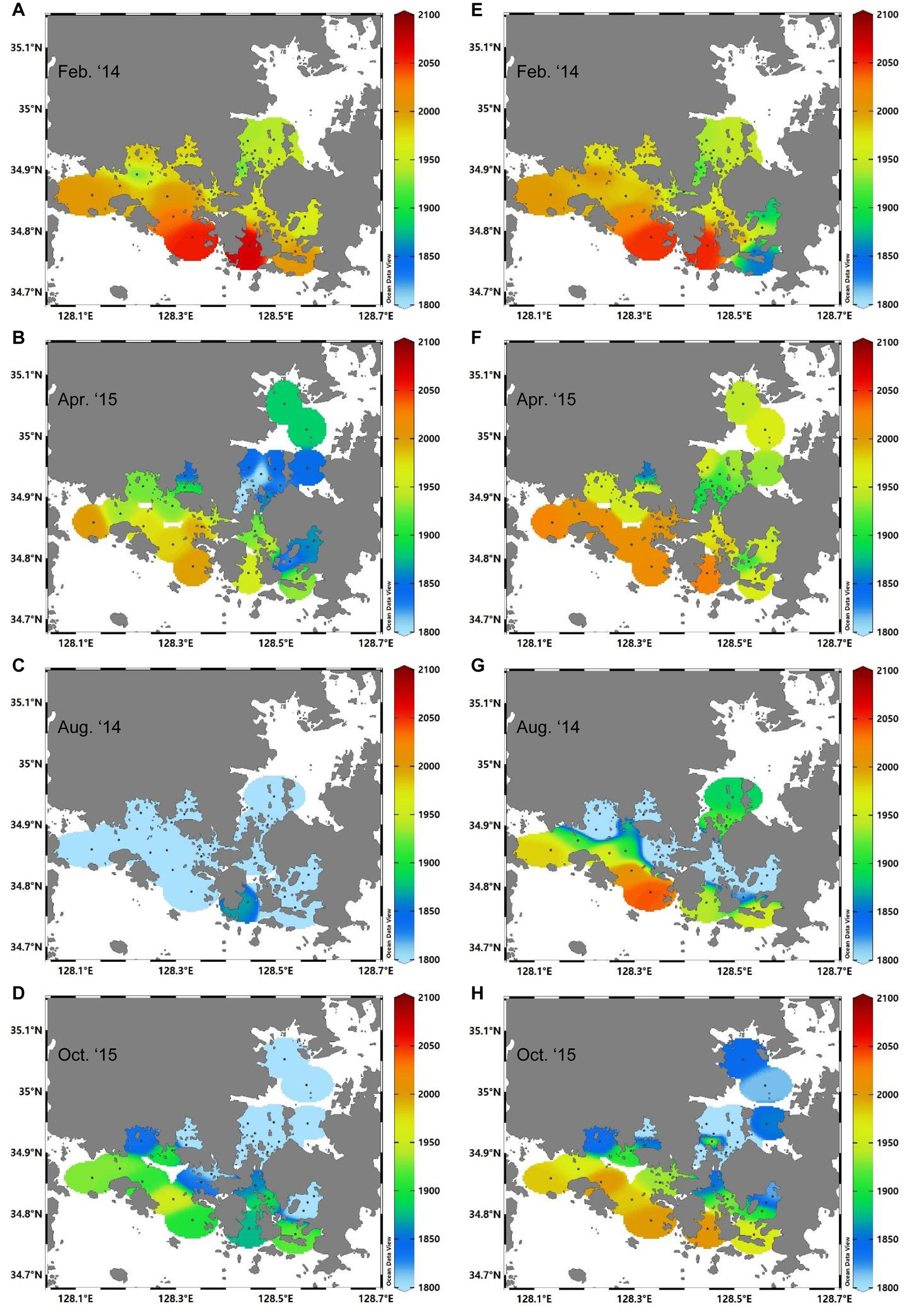
Figure 5. Distributions of dissolved inorganic carbon (DIC) (μmol kg^–1) in surface water (A–D) and bottom water (E–H) for each survey.

The values of the aragonite saturation state (Ω_Ar) in surface water and bottom water were similar (∼2.40) in February with relatively high values in Geoje Bay (2.9–3.1) (Table 1 and Figures 6A,E). In August, the Ω_Ar values of surface water and bottom water were 3.51 and 1.66, respectively (Figures 6C,G). Particularly, the value of surface water in outer area in area C ranged from 4.2 to 6.5, whereas that of bottom water ranged from 1.5 to 2.2. In April, the Ω_Ar of surface water was 2.40, which was similar to that in February, while that of bottom water was 2.15 (Figures 6B,F). In October, the Ω_Ar values of surface water and bottom water were 2.24 and 1.92, respectively (Figures 6D,H).

FIGURE 6

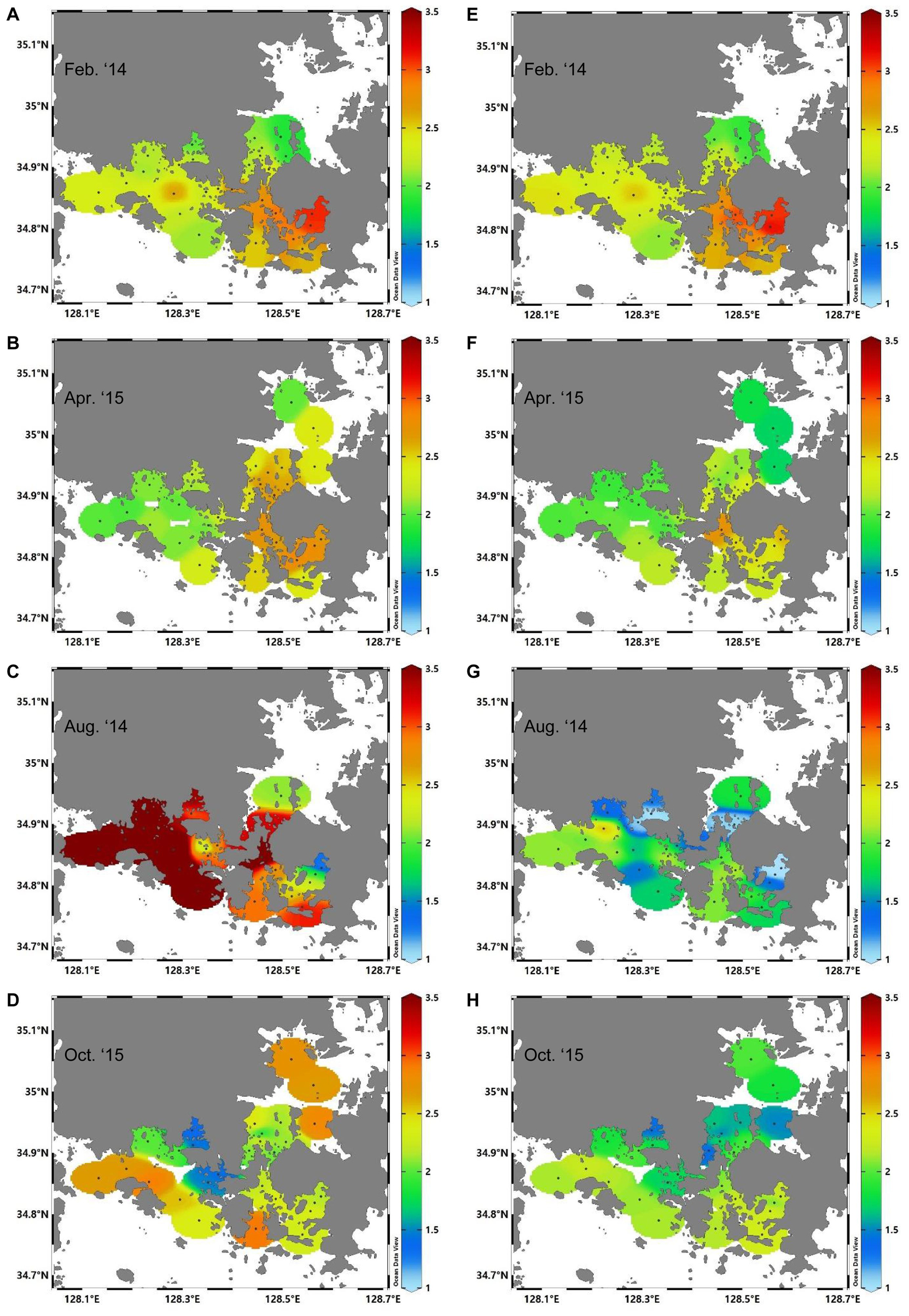
Figure 6. Distributions of aragonite saturation state (Ω_Ar) in surface water (A–D) and bottom water (E–H) for each survey. The dark red area in panel (C) had values of more than 3.5, hence the overrun in the same scale bar was applied in all figures for comparison.

In August, the mean nitrate concentrations in surface water and bottom water were 9.8 and 5.2 μmol kg^–1, respectively, which are 2–11 times higher than those in other periods (Table 1). The mean phosphate concentration was generally low (<0.5 μmol kg^–1) throughout the entire survey period, and was relatively high in February and October. The mean silicate concentration was relatively high in both April and August (15.8 and 12.8 μmol kg^–1, respectively), while it was maintained at approximately 7–9 μmol kg^–1 in February and October. Hence, the seasonal distribution trends were somewhat different for each nutrient. The mean chlorophyll-a concentration was relatively high in August (3.92 μg L^–1) and low (1.75 μg L^–1) in February (Table 1). In April and October, the mean chlorophyll-a concentration was similar (2.50 ± 0.17 μg L^–1) in surface water, while the mean value of bottom water was higher than of surface water in October (3.36 μg L^–1). In terms of the regional variation, the chlorophyll-a concentration was relatively high in the regions bordering areas A, B, and C and in Geoje Bay.

Discussion

Seasonal Variations of CO₂ and the Influencing Factors

The key factors affecting pCO₂ include temperature and salinity, physical mixing, biological factors, and air–sea exchange (Chou et al., 2017; Humphreys et al., 2018). In the mid-latitude waters of the North Pacific, which includes the study area, it has been reported that changes in the marine environment can be clearly observed in the typical seasonal variations. The seasonal variation of CO₂ in this region is larger than that at the equator or in the polar regions (Laruelle et al., 2017; Sutton et al., 2017). In the waters of the Kuroshio Extension Current in the mid-latitude region of the North Pacific Ocean, it has been reported that the seawater pCO₂ obtained from the Kuroshio Extension Observatory (KEO) mooring station showed typical seasonal variations of high values in summer and lower values in winter (ΔpCO₂ of ∼100 μatm), which was considered to be due to the large seasonality of sea surface temperatures (SSTs) and biological productivity. In contrast, in the Woods Hole Oceanographic Institution (WHOI) Hawaii Ocean Timeseries Station (WHOTS) and Stratus mooring stations in relatively low-latitude oligotrophic subtropical waters, Sutton et al. (2017) found small variations in SSTs and pCO₂ values (ΔpCO₂ of <30 and <50 μatm, respectively), with a lower correlation between SSTs and seawater pCO₂ compared with that of the KEO station.

In this study, in addition to the typical seasonal variations of mid-latitude regions, the area is subject to the effects of complex biogeochemical processes such as freshwater inflow from land, leading to complex actions on the spatiotemporal variability of CO₂. When examining the correlation between the CO₂ concentration and temperature and salinity of surface water in each survey period, no clear correlation was found for any of the four surveys (Figures 7A,C). Strong negative linear correlations were determined between the surface CO₂ concentration and pH during the entire study period (R² = 0.64) as well as during each survey period (Figure 7D). Spatial variations (2–3°C) were observed in the temperature data of each survey period. In February and April, the spatial variation in pCO₂ values was ∼100–150 μatm, while this increased to 300–500 μatm in August and October. In August, the CO₂ concentration was lower even in high-temperature waters. Therefore, it can be deduced that the spatial variation of CO₂ in each survey period was influenced by factors other than temperature. As described earlier, this was partly related to the different characteristics of waters in areas A, B, and C, while small bays did not experience uniform mixing due to limited circulation, and the impact from the adjacent inland areas was more significant. However, a positive correlation was observed between the CO₂ concentration and temperature for the entire study period. Except for August, which was the survey period with the largest spatial variation, there was a significant correlation between the CO₂ concentration and temperature (R² = 0.69) (Figure 7B).

FIGURE 7

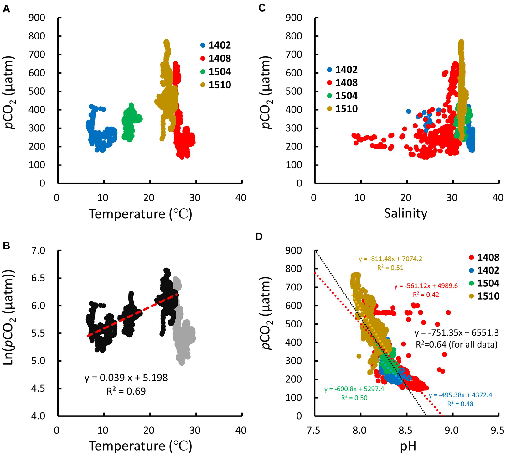
Figure 7. Plots of surface pCO₂ versus temperature (A,B), salinity (C), and pH (D) for each survey (dots: blue, Feb. 2014; red, Aug. 2014; green, Apr. 2015; dark yellow, Oct. 2015). In panel (B), the pCO₂ concentration is expressed as a logarithmic scale and is correlated except for August (gray).

Figure 7B compares our exponential correlation coefficient value between temperature and CO₂ (except for the value in August) of 0.039°C^–1 with the value of Takahashi et al. (1993) (0.0423°C^–1). Although the value of this study was relatively low, it was comparable, indicating that the temporal variation in the CO₂ concentration of surface seawater in the survey area relates primarily to the seasonal variation in temperature. As a result, the predicted pCO₂ (i.e., pCO₂ at T_obs) at the observed temperature was lower than the actual observed pCO₂ by approximately 30–50 μatm, but showed a similar seasonal variation (Figure 8). In August 2014, there was a considerable difference (∼180 μatm) between the predicted and observed pCO₂ values, with the former being higher, which was different from the results of other survey periods. The pCO₂ normalized to the mean temperature was ∼130 and ∼50 μatm higher than the actual observed pCO₂ values in February and April, respectively, whereas it was 80–90 μatm lower than the observed pCO₂ values in August and October. These results indicate that the effect of non-thermal factors on the increase in CO₂ was more dominant in February and April, while the effect of non-thermal factors on the decrease in CO₂ was more dominant in August and October. Although the mean seawater temperature and mean CO₂ concentration used in the previous calculations are appropriate for identifying the representative or typical trends of the relevant waters based on long-term observation data over several years or decades (Takahashi et al., 2002), this study only used the mean values of the results of four surveys. However, it is considered that it is still possible to identify the overall seasonal trends.

FIGURE 8

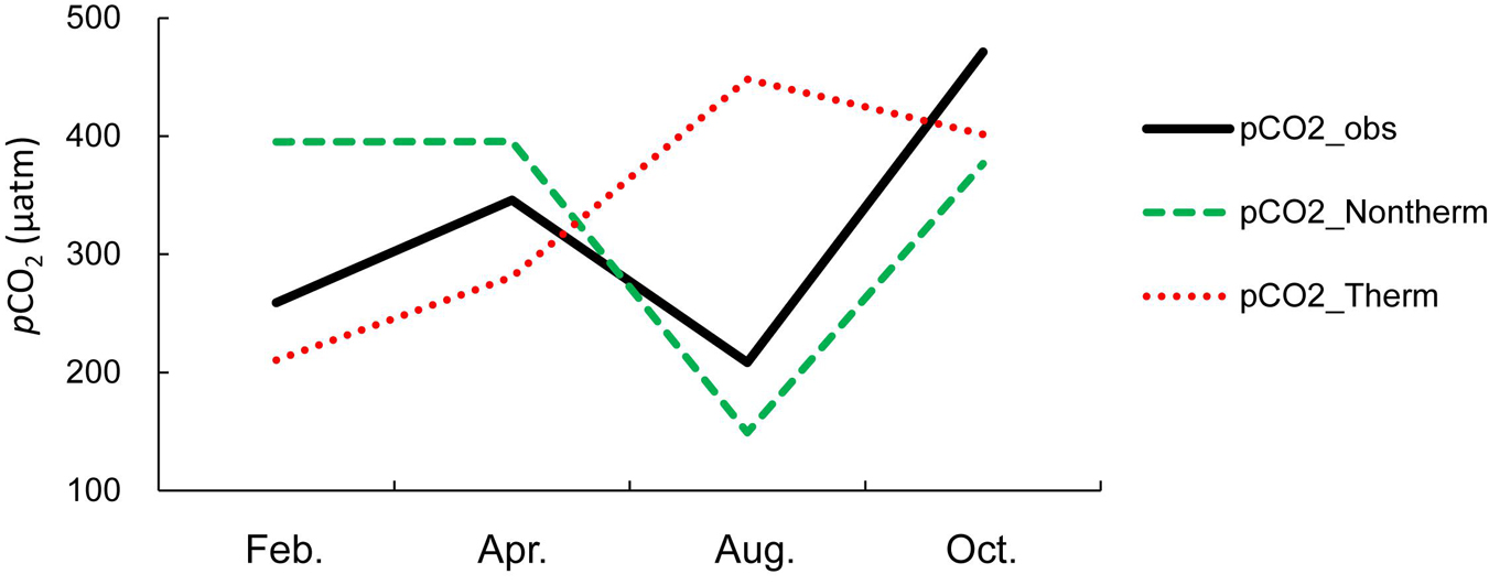
Figure 8. Drivers of seasonal variability in pCO₂ for each observed month. In situ values are shown with a solid black line. Dotted red lines show the pCO₂ variations caused by seasonal variations in temperature, whereas dashed green lines show the pCO₂ variations caused by non-thermal contributions.

In a previous study undertaken at the Great Barrier Reef in northeast Australia, it was found that the CO₂ concentration was mainly controlled by temperature in the wet season (when the temperature was relatively high), while both temperature and other factors controlled the CO₂ concentration in the dry season (when the temperature was relatively low) (Lønborg et al., 2019). In the northern Adriatic Sea, Urbini et al. (2020) found that temperature change was the dominant factor in summer, whereas the effect of biological processes was more dominant during other seasons. However, in August 2014, despite the high seawater temperature, the observed CO₂ concentrations were relatively low, the spatial variability was considerably large, and the pCO₂ results showed a significant deviation from the range of seasonal variability caused by temperature typically observed during the summer season in mid-latitude waters. This indicates that the effect of other non-thermal marine environmental factors was more dominant than that of temperature change.

The coastal waters in Yeosu-Tongyeong on the southeastern coast of Korea are areas that experience frequent red tide events in summer. This was especially the case in 2014, when a red tide watch (>100 cells mL^–1 of M. polykrikoides) was issued for the first time on July 31 in Goseong (area C in this study), followed by a red tide warning (>1000 cells mL^–1) on August 19 in the coastal waters of the Jinhae–Geoje–Tongyeong bay area (National Fisheries Research and Development Institute, 2014). This change to more critical alert was probably related to the typhoon that occurred between August 1 and 3, which created an ideal environment for the active growth of phytoplankton due to the nutrients introduced from the land along with heavy rain. In fact, the amount of rainfall in August 2014 was approximately 590 mm, which was nearly twice the 25-year mean rainfall for August (254 mm) (Korea Meteorological Administration, 2021). In addition, as a result of the surveys on August 5 and August 28 at the hypoxia survey station (H12, Figure 1) in JB (area A), the chlorophyll-a concentration increased rapidly from 2.0 to 33.0 μg L^–1, respectively, while the nitrate (ammonium) and phosphate concentrations decreased from 16.1(4.6) to 13.4(0.5) μmol kg^–1 and 0.50 to 0.04 μmol kg^–1, respectively (Korea Oceanographic Data Center, 2021). This sharp increase in chlorophyll-a (16.5-fold) that was simultaneous to decreases in nutrient concentrations indicates the rapid growth of phytoplankton and plankton associated with red tides, thereby reducing the CO₂ concentration and increasing DO and pH of seawater through photosynthesis. Moreover, the mean phytoplankton abundance during the regular red tide monitoring, particularly, around area A of 14 stations was 34 cells mL^–1 in July, which rapidly increased by 10-folds to cell density of 343 cells mL^–1 in August, and finally decreased to 109 cells mL^–1 in September (Korea Oceanographic Data Center, 2021; Supplementary Table 1). The surface DO at the hypoxia station (H12) increased from 6.53 (saturation rate of 96%) to 10.17 (saturation rate of 140%) mg L^–1, and the pH increased from 7.98 to 8.50 over 23 days, thus supporting the above analysis.

In August 2014, the decrease in CO₂ due to the significant increase in the production of red tide phytoplankton was large enough to counteract the increase due to the seawater temperature. In particular, the duration and damage to fisheries due to the red tide event (harmful algae bloom by M. polykrikoides) in 2014 were the longest (∼80 d, from July 31 to October 17) and the 6th highest (economic loss of 7.4 billion KRW), respectively, among the red tide events in Korea since 1995 (National Fisheries Research and Development Institute, 2014). During our survey in August, a red tide patch was clearly observed in JB of area A. However, red tide events along the Korean coast have continuously decreased since the mid-1990s, and the frequency of red tide events and major red tide species has changed in recent years because temperatures have increased (≥28°C) as a result of climate change and nutrients have decreased (Lim et al., 2020; Sakamoto et al., 2021). During 2016–2020, the seawater temperature in the study area exceeded the optimum growth temperature (23–25°C) of M. polykrikoides, a major red tide organism, and the frequency of red tide events reduced compared with that of previous years. However, the relationships between the increase in seawater temperature and growth and toxicity of harmful algal bloom (HAB) species are highly strain- and species-specific, for example, maximum growth rate of M. polykrikoides was observed at 24–27°C, and the toxicity was stronger in cultures maintained at 16–25°C (Griffith and Gobler, 2020). Two different strains (CP2013 and CP2018) of M. polykrikoides in Korean Coastal water exhibited a considerably different growth responses to high water temperature; CP2013 did not survive above 28°C, whereas CP2018 could grow (Lim et al., 2021). The severe influence of massive red tides was expected in the past, and our study revealed that Margalefidinium blooms primarily governed the summer pCO₂ variations; however, it is considered that the influence of red tides on pCO₂ variations in the summer will be reduced or the timing of the HABs-driven pCO₂ variation will be shifted to earlier season as blooms will occur earlier and hotter under the varying environmental conditions (Griffith and Gobler, 2020; Lim et al., 2020, 2021).

The predicted CO₂ concentration without the effect red tide events could be calculated for August 2014 using the correlation between the CO₂ concentration and temperature in Figure 7B. Substituting the mean temperature in August (26.72°C), the estimated pCO₂ was approximately 512 μatm, and the value also calculated using the mean pCO₂ in Eq. 2 was >472 μatm, which are 180–220 μatm higher than the observed value of 293 μatm. In fact, considering that the results calculated using the input value (mean annual pCO₂) of Eq. 2 including the unusually low pCO₂ value in August may be underestimated, it can be inferred that the pCO₂ value decreased by ∼200 μatm due to primary production associated with the red tide event. It is unknown whether the reduction in the CO₂ concentration caused by the primary production of red tide organisms is maintained throughout the duration of a red tide event. However, this survey was conducted approximately 22–25 days after the first red tide report (31 July), and the measurements were made after the survey at the hypoxia station; hence, it is inferred that the survey period coincided with the peak primary production of red tide organisms. The mean phytoplankton abundance at special red-tide monitoring stations in the Tongyeong–Geoje Bay area peaked from the end of August to beginning of September, with cell density approximately doubling from 478 cells mL^–1 on August 18 to 830 cells mL^–1 on September 1, and then rapidly decreased to 220 cells mL^–1 on September 15 (Korea Oceanographic Data Center, 2021; Supplementary Table 2). Therefore, a reduction in the CO₂ concentration on this scale following a significant increase in primary production due to the red tide event is one aspect of the complex biogeochemical cycle of the coastal region, and makes a significant contribution to the carbon cycle.

Air–Sea Surface CO₂ Flux and the Carbonate Saturation State of the Water Column

The mid-latitude coastal zones are considered regions of CO₂ uptake, but the scale of this uptake remains controversial. The air–sea flux of CO₂ calculated using the data from this study indicated the uptake of atmospheric CO₂ by seawater in all survey periods except October 2015, when seawater was a source of CO₂ (3.7 mmol m^–2 d^–1) (Figure 9). The most efficient uptake was in February 2014 (14.2 mmol m^–2 d^–1), followed by August and April. Despite the fact that the surface pCO₂ was higher in February than in August 2014, the highest uptake flux occurred in February because the atmospheric CO₂ concentration was ∼10 μatm higher than that in August, and the mean wind speed, which affects the air–sea CO₂ flux, was probably also larger. In February, the air–sea flux of CO₂ was ≥−16.0 mmol m^–2 d^–1 in area B, which was the most efficient CO₂ uptake value of all areas during the survey period. In August and April, the most efficient CO₂ uptake was observed in area A. In October, the largest CO₂ emissions were observed in area C, especially in small bays such as Goseong, Jaran, and Bukshin bays, with flux values of ≥15 mmol m^–2 d^–1. The average air–sea flux of CO₂ for 4 surveys was about −5.24 mmol m^–2 d^–1 for the whole study area, suggesting an effective sink area compared to other costal sea and continental shelf (Chen et al., 2013; Roobaert et al., 2019). Shim et al. (2007) reported that the air–sea flux of CO₂ in the northern East China Sea ranged seasonally from −5.04 to 0.39 mmol m^–2 d^–1, whereby the area acted as a weak source in autumn, with an estimated annual average of −2.37 mmol m^–2 d^–1, a much less effective uptake rate than our value.

FIGURE 9

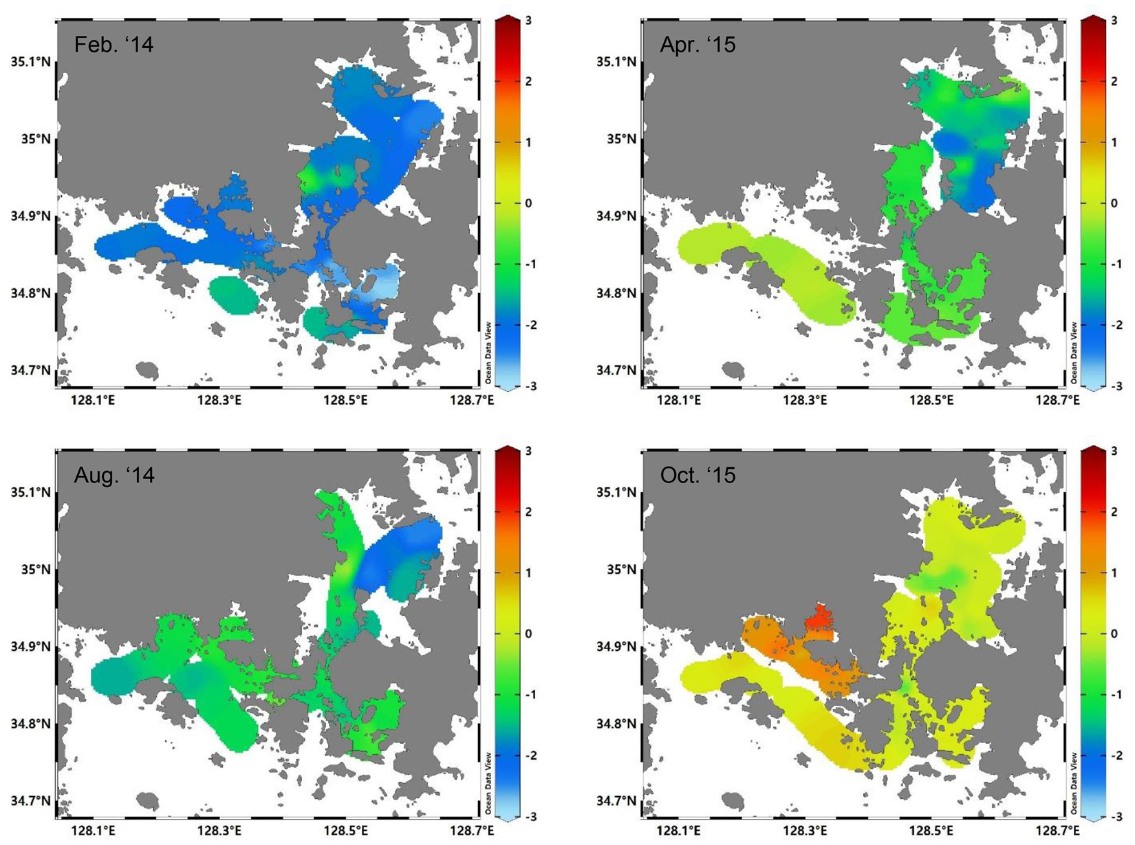
Figure 9. Distributions of air-sea CO₂ exchange flux (mmol m^–2 d^–1) for each survey. A positive value indicates a flux direction from sea to air, that is, the sea acts as a CO₂ source, whereas a negative value indicates the opposite.

As discussed previously, there was a strong red tide event in the study area in 2014. Thus, the area acted as a CO₂ sink even in August, the representative month of summer; however, this cannot be regarded as a general trend. Therefore, the annual CO₂ concentration and flux of the study area were estimated under the following assumptions: the CO₂ concentration is mainly affected by seasonal variations in temperature, and the extent of the effect is the value obtained from the aforementioned correlation between the CO₂ concentration and seawater temperature (δlnpCO₂/δT = 0.039°C^–1). A quadratic equation was applied to estimate the monthly temperature change, using the regular monitoring around the aquaculture area of Jinhae–Geoje–Tongyeong conducted every even month from 2011 to 2015 by NIFS (Korea Oceanographic Data Center, 2021). Moreover, the mean monthly wind speed and atmospheric CO₂ concentration observed by KMA were used as in the section “Materials and Methods” (Korea Meteorological Administration, 2021).

Accordingly, the calculated CO₂ uptake flux of seawater in the coastal waters of area A ranged from 2.9 to 17.2 mmol m^–2 d^–1 between November and May (Table 2 and Figure 10). In June, the CO₂ budget was balanced, while CO₂ emission values of 1.4–3.2 mmol m^–2 d^–1 were obtained between July and October. The annual mean flux was −5.64 mmol m^–2 d^–1, indicating an efficient uptake of atmospheric CO_2. In the coastal waters of areas B and C, CO₂ uptake fluxes were determined between November and July, whereas seawater acted as a source of CO₂ to the atmosphere between July and October. The annual mean flux was similar between the two areas at −4.7 and −4.9 mmol m^–2 d^–1, respectively. In area A, the highest CO₂ uptake value was in February (−17.2 mmol m^–2 d^–1), while the highest emission values were in August and September (≥3.2 mmol m^–2 d^–1). This is because area A had a lower (higher) seawater temperature in winter (summer) than areas B and C, which are adjacent to the open ocean and experience a higher seasonal variation in temperatures. Therefore, the mean air–sea CO₂ flux of the entire study area was approximately −5.1 mmol m^–2 d^–1, and when substituting the area (∼719 km²), the annual uptake was equivalent to 16 × 10⁶ kg of C. However, in the abovementioned assumptions, the strong CO₂ uptake event due to the red tide and blooms as in August 2014 was not included, and thus the actual uptake was probably larger than this value. In addition, National Institute of Fisheries Science (2019) reported that the mean temperature in the seas around the Korean Peninsula rose by 1.23°C (0.0241°C y^–1) over 51 years (1968–2018), and that the mean increase on the southeastern coast was slightly lower at 1.03°C (0.0202°C y^–1). When the reported values and predicted rate of temperature increase in 2050 were applied, the air–sea CO₂ flux reduced to −4.5 mmol m^–2 d^–1, indicating a decrease of ∼11.5% in the CO₂ uptake efficiency compared with 2014–2015. However, this is based on the assumption that the atmospheric CO₂ concentration did not increase. If it did increase by 2.37 μatm y^–1 (as is the current trend; WMO, 2020), the rate of increase of the air–sea CO₂ flux would be higher than the rate of increase of marine CO₂ due to the temperature rise, with an air–sea CO₂ flux of −9.6 mmol m^–2 d^–1, which could increase the carbon uptake rate by >50% compared with the present rate.

TABLE 2

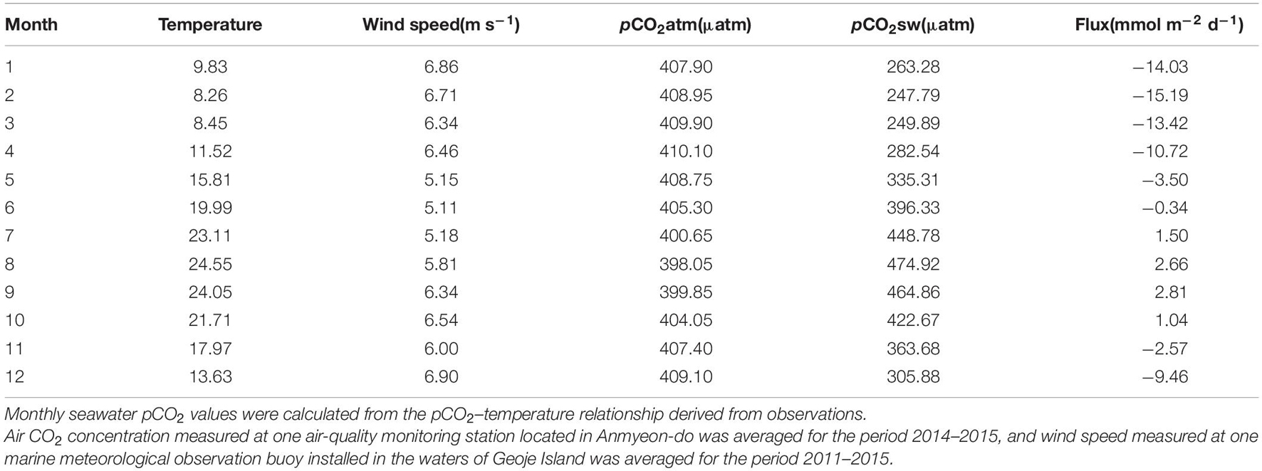
Table 2. Monthly values of calculated air-sea CO₂ flux and related parameters.

FIGURE 10

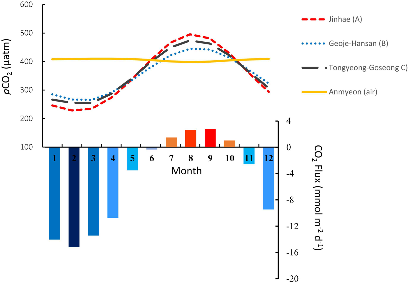
Figure 10. Monthly variation of pCO₂ in seawater for the three bay areas (dotted and dashed lines) and in the atmosphere at Anmyeon-do (solid line), and CO₂ flux of the study area (bars). Surface seawater pCO₂ was calculated from the observed pCO₂-temperature relationship and monthly temperature variation at each area, derived from expectations using 5 years of even month observations.

Although the difference in certain environmental parameters between surface water and bottom water is not significant in the studied coastal region because of the shallow water depth, it is important to identify the distribution of carbonate factors in the water column for a precise understanding of the carbon cycle. In particular, considering that seasonal hypoxia occurs in the bottom water of the study area, it is highly likely that the distribution characteristics differ from those of the surface water.

The DIC concentration also exhibited a high correlation with salinity in each survey period and over the entire study period (Figures 11A,B). In surface water, the correlation was relatively low in February, whereas it was high in April, August, and October (R² > 0.6), and for the entire study period (R² = 0.81). The correlation between the DIC concentration and salinity of bottom seawater was ≥0.5 in all survey periods except February, while it was 0.6 for the entire study period.

FIGURE 11

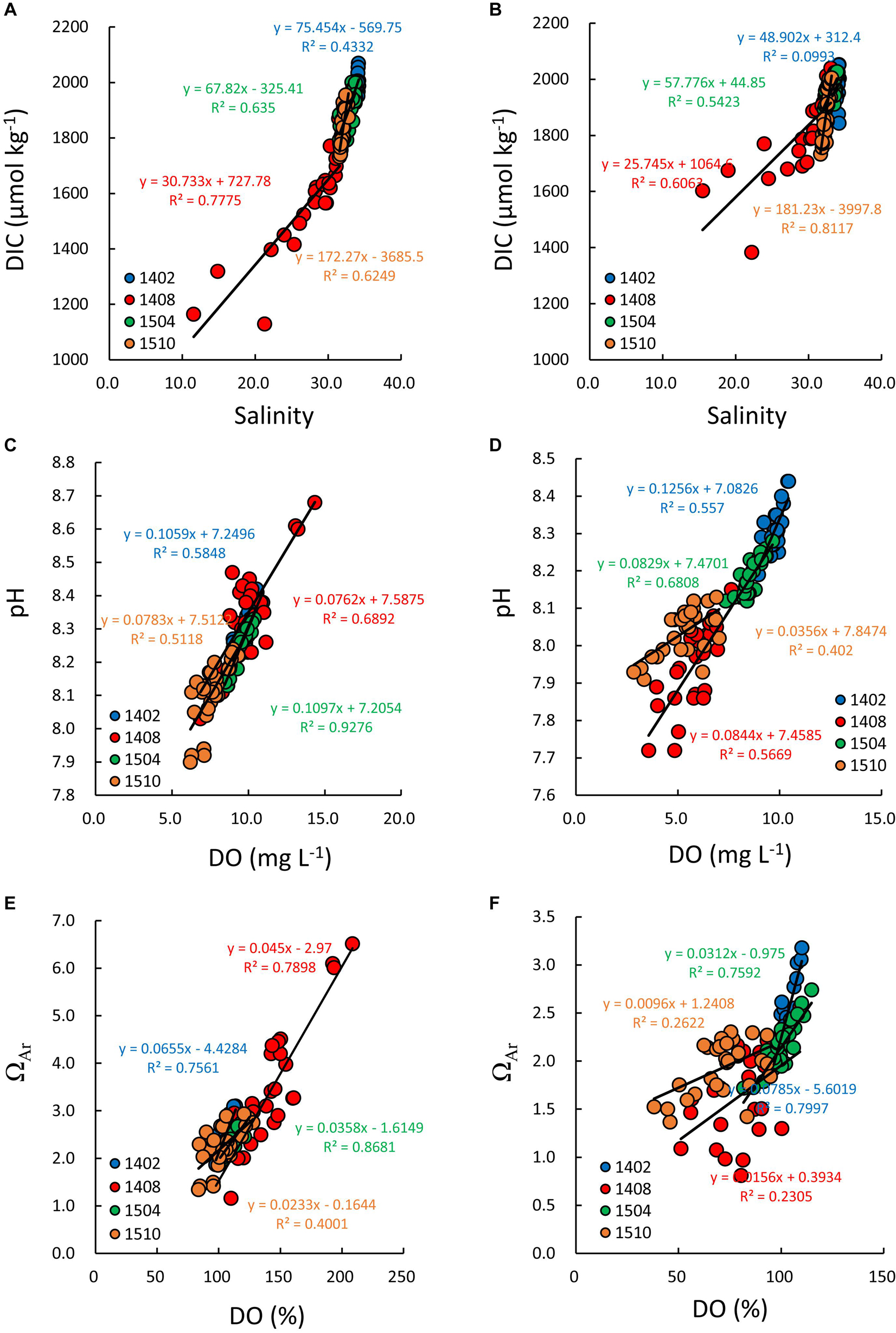
Figure 11. Plots of salinity versus DIC in surface water (A) and bottom water (B), dissolved oxygen (DO) versus pH in surface (C) and bottom (D) water, and DO (%) versus Ω_Ar surface (E) and bottom (F) water for each survey (dots: blue, Feb. 2014; red, Aug. 2014; green, Apr. 2015; dark yellow, Oct. 2015).

When observing the data of the entire survey period at a glance, the pH of seawater was generally higher at lower temperatures and higher salinity. Except for August, high correlations were found between pH and temperature (0.77) and pH and salinity (0.56) in bottom water. These findings relate to the formation of strong stratification in the water column when the surface temperature was high, thus reducing the oxygen supply to bottom water. The pH was lowered because of the transition from oxidizing to reducing conditions. In addition, if salinity is low due to freshwater inflow from land, stratification is also reinforced, which is thought to have led to the correlation with salinity. Therefore, there were high correlations between pH and DO in both surface and bottom water for entire (R² = 0.79) and each survey period (Figures 11C,D).

The values of the aragonite saturation state (Ω_Ar) showed high correlations with the DO saturation state for the entire survey period in surface water (R² = 0.78), and in February 2014 and April 2015 in bottom water (Figures 11E,F). In August and October, the Ω_Ar values of bottom water showed low relationships with DO saturation, suggesting that the additional DO consumption caused by decomposition of the organic matter might have been a contributing factor to the lowering DO concentration at some stations. Kim et al. (2013) also suggested that most of the bottom waters in JB were undersaturated with respect to aragonite during the summer of 2011, caused by active biological production in the water column and was followed by decomposition at the sediment–water interface. Every year, active oyster farming is performed in the study region from September to April–May of the following year, thus if the Ω_Ar value decreases to ≤1, there will be a significant negative impact on the oyster aquaculture industry in this area. Therefore, although the Ω_Ar values of surface water can reach 2–3 in August and October, the low Ω_Ar values (<2) in bottom water are of great concern because that is the time of reproduction and growth of juvenile oysters (i.e., the initial stage of oyster farming). In most of these waters, the depth is <20 m and the submerged longline of oyster farming can be up to 10 m; thus, low Ω_Ar values in bottom water can have a substantial impact on oyster farming. This is because the mixing between surface water and bottom water is limited due to stratification owing to the density difference between them. Actually, high Ω_Ar values in surface water (3.0–4.5) with super-saturated DO conditions (130–160%) occurred particularly at stations in TGB (area C), whereas low Ω_Ar values in bottom water were generally observed. In the northern East China Sea in July 2018, low Ω_Ar values (1.21–1.39) were observed along with hypoxia-level DO values (about 1.5–2.0 mg kg^–1) (Xiong et al., 2020). Considering the possible future conditions of the study area, a further increase in seawater temperatures under climate change would be expected to increase stratification, leading to an even larger difference in the Ω_Ar values between surface and bottom water. This finding warrants further investigation of the intensive impacts of low carbonate saturation states on the oyster industry.

Data Availability Statement

The raw data supporting the conclusions of this article will be made available by the authors, without undue reservation.

Author Contributions

JS designed the research and performed the field surveys. M-JY and JK analyzed the data set and drafted an early version of the manuscript. J-HL and J-NK contributed to the data collection and visualization. All authors contributed to discussion and revision of the manuscript.

Funding

This research was supported by the National Institute of Fisheries Sciences R&D project (R2021032).

Conflict of Interest

M-JY was employed by the company BLTEC Korea Limited.

The remaining authors declare that the research was conducted in the absence of any commercial or financial relationships that could be construed as a potential conflict of interest.

Publisher’s Note

All claims expressed in this article are solely those of the authors and do not necessarily represent those of their affiliated organizations, or those of the publisher, the editors and the reviewers. Any product that may be evaluated in this article, or claim that may be made by its manufacturer, is not guaranteed or endorsed by the publisher.

Supplementary Material

The Supplementary Material for this article can be found online at: https://www.frontiersin.org/articles/10.3389/fmars.2021.738472/full#supplementary-material

References

Bates, N. R., Astor, Y. M., Church, M. J., Currie, K., Dore, J. E., and González-Dávila, M. (2014). A time-series view of changing ocean chemistry due to ocean uptake of anthropogenic CO₂ and ocean acidification. Oceanogrphy 27, 126–141. doi: 10.5670/oceanog.2014.16

CrossRef Full Text | Google Scholar

Carstensen, J., Chierice, M., Gustafsson, B. G., and Gustafsson, E. (2018). Long-term and seasonal trends in estuarine and coastal carbonate systems. Glob. Biogeochem. Cycles 32, 497–513. doi: 10.1002/2017GB005781

CrossRef Full Text | Google Scholar

Chen, C.-T. A., Huang, T.-H., Chen, Y.-C., Bai, Y., He, X., and Kang, Y. (2013). Air-sea exchanges of CO₂ in the world’s coastal seas. Biogeosciences 10, 6509–6544. doi: 10.5194/bg-10-6509-2013

CrossRef Full Text | Google Scholar

Cho, Y.-S., Lee, W.-C., Hong, S.-J., Kim, H.-C., Kim, J.-B., and Park, J.-H. (2012). Estimation of stocking density using habitat suability index and ecological indicator for oyster farms in Geoje-Hansan Bay. J. Korean Soc. Mar. Environ. Saf. 18, 185–191. doi: 10.7837/kosomes.2012.18.3.185

CrossRef Full Text | Google Scholar

Chou, W.-C., Tishchenko, P. Y., Chuang, K.-Y., Gong, G.-C., Shkirmikova, E. M., and Tishchenko, P. P. (2017). The controlling behaviors of CO₂ systems in river-dominated and ocean-dominated continental shelves: a case study in the East China Sea and the Peter the Great Bay of the Japan/East Sea in summer 2014. Mar. Chem. 195, 50–60. doi: 10.1016/j.marchem.2017.04.005

CrossRef Full Text | Google Scholar

Dickson, A. G., Sabine, C. L., and Christian, J. R. (2007). Guide to best practices for ocean CO₂ measurements. PICES Special Publ. 3:191.

Google Scholar

Duarte, C. M., Hendriks, I. E., Moore, T. S., Olsen, Y. S., Steckbauer, A., Ramajo, L., et al. (2013). Is ocean acidification an open-ocean syndrome? Understanding anthropogenic impacts on seawater pH. Estuaries Coast. 36, 221–236. doi: 10.1007/s12237-013-9594-3

CrossRef Full Text | Google Scholar

Griffith, A. W., and Gobler, C. J. (2020). Harmful algal blooms: a climate change co-stressor in marine and freshwater ecosystems. Harmful Algae 91:101590. doi: 10.1016/j.hal.2019.03.008

PubMed Abstract | CrossRef Full Text | Google Scholar

Gruber, N. (2015). Carbon at the costal interface. Nature 517, 148–149. doi: 10.1038/nature14082

PubMed Abstract | CrossRef Full Text | Google Scholar

Hoegh-Guldberg, O., Mumby, P. J., Hooten, A. J., Steneck, R. S., Greenfield, P., Gomez, E., et al. (2007). Coral reefs under rapid climate change and ocean acidification. Science 318, 1737–1742. doi: 10.1126/science.1152509

PubMed Abstract | CrossRef Full Text | Google Scholar

Humphreys, M. P., Daniels, C. J., Wolf-Gladrow, D. A., Tyrrell, T., and Achterberg, E. P. (2018). On the influence of marine biogeochemical processes over CO₂ exchange between the atmosphere and ocean. Mar. Chem. 199, 1–11. doi: 10.1016/j.marchem.2017.12.006

CrossRef Full Text | Google Scholar

IPCC (2014). “Climate change 2014: synthesis report,” in Contribution of Working Groups I, II and III to the Fifth Assessment Report of the Intergovernmental Panel on Climate Change, eds Core Writing Team, R. K. Pachauri, and L. A. Meyer (Geneva: IPCC), 151.

Google Scholar

Jiang, Z.-P., Cai, W.-J., Chen, B., Wang, K., Han, C., Roberts, B. J., et al. (2019). Physical and biogeochemical controls on pH dynamics in the Northern Gulf of Mexico during summer hypoxia. J. Geophys. Res. 124, 5979–5998. doi: 10.1029/2019JC015140

CrossRef Full Text | Google Scholar

Kim, D., Choi, S.-H., Yang, E.-J., Kim, K.-H., Jeong, J.-H., and Kim, Y. O. (2013). Biologically mediated seasonality of aragonite saturation states in Jinhae Bay, Korea. J. Coast. Res. 29, 1420–1426. doi: 10.2112/JCOASTRES-D-12-00205.1

CrossRef Full Text | Google Scholar

Kim, D., Park, G.-H., Baek, S. H., Choi, Y., and Kim, T.-W. (2018). Physical and biological control of aragonite saturation in the coastal waters of southern South Korea under the influence of freshwater. Mar. Pollut. Bull. 129, 318–328. doi: 10.1016/j.marpolbul.2018.02.038

PubMed Abstract | CrossRef Full Text | Google Scholar

Kim, J.-Y., Kang, D.-J., Lee, T., and Kim, K.-R. (2014). Long-term trend of CO₂ and ocean acidification in the surface water of the Ulleung Basin, the East/Japan Sea inferred from the underway observational data. Biogeosciences 11, 2443–2454. doi: 10.5194/bg-11-2443-2014

CrossRef Full Text | Google Scholar

Korea Meteorological Administration (2021). KMA Weather Data Service Open MET Data Portal. Available online at: https://data.kma.go.kr/ (accessed May 10, 2021).

Google Scholar

Korea Oceanographic Data Center (2021). Red Tide Information System and Environmental Monitoring at Fishery Farm. Available online at: https://www.nifs.go.kr/kodc/index.kodc (accessed January 8, 2021).

Google Scholar

KOSIS (2021). Fishery Production Survey. Available online at: https://kosis.kr/ (accessed May 14, 2021).

Google Scholar

Kroeker, K. J., Kordas, R. L., Crim, R., Hendriks, I. E., Ramajo, L., Singh, G. S., et al. (2013). Impacts of ocean acidification on marine organisms: quantifying sensitivities and interaction with warming. Glob. Chang. Biol. 19, 1884–1896. doi: 10.1111/gcb.12179

PubMed Abstract | CrossRef Full Text | Google Scholar

Kwon, J.-N., Lee, J., Kim, Y., Lim, J.-H., Choi, T.-J., Ye, M.-J., et al. (2014). Long-term variations of water quality in Jinhae Bay. J. Korean Soc. Mar. Environ. Energy 17, 324–332. doi: 10.7846/JKOSMEE.2014.17.4.324

CrossRef Full Text | Google Scholar

Laruelle, G. G., Landschützer, P., Gruber, N., Tison, J.-L., Delille, B., and Regnier, P. (2017). Global high-resolution monthly pCO₂ climatology for the coastal ocean derived from neural network interpolation. Biogeosciences 14, 4545–4561. doi: 10.5194/bg-14-4545-2017

CrossRef Full Text | Google Scholar

Laruelle, G. G., Lauerwald, R., Pfeil, B., and Regnier, P. (2014). Regionalized global budget of the CO₂ exchange at the air-water interface in continental shelf seas. Glob. Biogeochem. Cycles 28, 1199–1214. doi: 10.1002/2014GB004832

CrossRef Full Text | Google Scholar

Le Quéré, C., Andrew, R. M., Friedlingstein, P., Sitch, S., Hauch, J., Pongratz, J., et al. (2018). Global carbon budget 2018. Earth Syst. Sci. Data 10, 2141–2194. doi: 10.5194/essd-10-2141-2018

CrossRef Full Text | Google Scholar

Lee, J., Park, K.-T., Lim, J.-H., Yoon, J.-E., and Kim, I.-N. (2018). Hypoxia in Korean coastal waters: a case study of the natural Jinhae Bay and artificial Shiwa Bay. Front. Mar. Sci. 5:70. doi: 10.3389/fmars.2018.00070

CrossRef Full Text | Google Scholar

Lim, W.-A., Go, W.-J., Kim, K.-Y., and Park, J.-W. (2020). Variation in harmful algal blooms in Korean coastal waters since 1970. J. Korean Soc. Mar. Environ. Saf. 26, 523–530. doi: 10.7837/kosomes.2020.26.5.523

CrossRef Full Text | Google Scholar

Lim, Y. K., Park, B. S., Kim, J. H., Baek, S.-S., and Baek, S. H. (2021). Effect of marine heatwaves on bloom formation of the harmful dinoflagellate Cochlodinium polykrikoides: two sides of the same coin? Harmful Algae 104:102029. doi: 10.1016/j.hal.2021.102029

PubMed Abstract | CrossRef Full Text | Google Scholar

Lønborg, C., Calleja, M. L., Fabricius, K. E., Smith, J. N., and Achterberg, E. P. (2019). The great barrier reef: a source of CO₂ to the atmosphere. Mar. Chem. 210, 24–33. doi: 10.1016/j.marchem.2019.02.003

CrossRef Full Text | Google Scholar

MOF (2013). Standard Method for the Analysis of Marine Environment. Available online at: https://www.law.go.kr/admRulLsInfoP.do?admRulSeq=2000000109042 (accessed December 30, 2013).

Google Scholar

National Fisheries Research and Development Institute (2014). Harmful Algal Blooms in Korean Coastal Waters in 2014. Busan: GMK Communication.

Google Scholar

National Institute of Fisheries Science (NIFS) (2019). Assessment Report on Fisheries Impacts in a Changing Climate. Busan: Maple Design.

Google Scholar

Pierrot, D., Lewis, E., and Wallace, D. W. R. (2006). MS Excel Program Developed for CO2 System Calculations. ORNL/CDIAC-105a. Oak Ridge, TN: Carbon Dioxide Information Analysis Center, Oak Ridge National Laboratory, U.S. Department of Energy. doi: 10.3334/CDIAC/otg.CO2SYS_XLS_CDIAC105a

CrossRef Full Text | Google Scholar

Pilcher, D. J., Naiman, D. M., Cross, J. N., Hermann, A. J., Siedlecki, S. A., Gibson, G. A., et al. (2019). Modeled effect of coastal biogeochemical processes, climate variability, and ocean acidification on aragonite saturation state in the Bering Sea. Front. Mar. Sci. 5:508. doi: 10.3389/fmars.2018.00508

CrossRef Full Text | Google Scholar

Roobaert, A., Laruelle, G. G., Landschützer, P., Gruber, N., Chou, L., and Regnier, P. (2019). The spatiotemporal dynamics of the sources and sinks of CO₂ in the global coastal ocean. Glob. Biogeochem. Cycles 33, 1693–1714. doi: 10.1029/2019GB006239

CrossRef Full Text | Google Scholar

Sakamoto, S., Lim, W. A., Lu, D., Dai, X., Orlova, T., and Iwataki, M. (2021). Harmful algal blooms and associated fisheries damage in East Asia: current status and trends in China, Japan, Korea and Russia. Harmful Algae 102:101787. doi: 10.1016/j.hal.2020.101787

PubMed Abstract | CrossRef Full Text | Google Scholar

Shim, J. H., Kim, D., Kang, Y. C., Lee, J. H., Jang, S.-T., and Kim, C.-H. (2007). Seasonal variations in pCO₂ and its controlling factors in surface seawater of the northern East China Sea. Cont. Shelf Res. 27, 2623–2636. doi: 10.1016/j.csr.2007.07.005

CrossRef Full Text | Google Scholar

Sutton, A. J., Wanninkhof, R., Sabine, C. L., Feely, R. A., Cronin, M. F., and Weller, R. A. (2017). Variability and trends in surface seawater pCO₂ and CO₂ flux in the Pacific Ocean. Geophys. Res. Lett. 44, 5627–5636.

Google Scholar

Takahashi, T., Olafsson, J., Goddard, J. G., Chipman, D. W., and Sutherland, S. C. (1993). Seasonal variation of CO₂ and nutrients in the high-latitude surface oceans: a comparative study. Glob. Biogeochem. Cycles 7, 843–878. doi: 10.1029/93GB02263

CrossRef Full Text | Google Scholar

Takahashi, T., Sutherland, S. C., Sweeney, C., Poisson, A., Metzl, N., Tilbrook, B., et al. (2002). Global sea-air CO₂ flux based on climatological surface ocean pCO₂, and seasonal biological and temperature effects. Deep Sea Res. II 49, 1601–1622. doi: 10.1016/S0967-0645(02)00003-6

CrossRef Full Text | Google Scholar

Urbini, L., Ingrosso, G., Djakovac, T., Piacentino, S., and Giani, M. (2020). Temporal and spatial variability of the CO₂ system in a riverine influenced area of the Mediterranean Sea, the Northern Adriatic. Front. Mar. Sci. 7:679. doi: 10.3389/fmars.2020.00679

CrossRef Full Text | Google Scholar

Waldbusser, G. G., Powell, E. N., and Mann, R. (2013). Ecosystem effects of shell aggregations and cycling in coastal waters: an example of Chesapeake Bay oyster reefs. Ecology 94, 895–903.

Google Scholar

Wallace, R. B., Baumann, H., Grear, J. S., Aller, R. C., and Gobler, C. J. (2014). Coastal ocean acidification: the other eutrophication problem. Estuar. Coast. Shelf Sci. 148, 1–13. doi: 10.1016/j.ecss.2014.05.027

CrossRef Full Text | Google Scholar

Wanninkhof, R. (1992). Relationship between wind speed and gas exchange over the ocean. J. Geophys. Res. 97, 7373–7382. doi: 10.1029/92JC00188

CrossRef Full Text | Google Scholar

Wanninkhof, R. (2014). Relationship between wind speed and gas exchange over the ocean revisited. Limnol. Oceanogr. Meth. 12, 351–362. doi: 10.4319/lom.2014.12.351

CrossRef Full Text | Google Scholar

Weiss, R. F. (1974). Carbon dioxide in water and seawater: the solubility of a non-ideal gas. Mar. Chem. 2, 203–215. doi: 10.1016/0304-4203(74)90015-2

CrossRef Full Text | Google Scholar

WMO (2020). Greenhouse Gas Bulletin No.16. 9. Geneva: WMO.

Google Scholar

Xiong, T., Wei, Q., Zhai, W., Li, C., Wang, S., Zhang, Y., et al. (2020). Comparing subsurface seasonal deoxygenation and acidification in the Yellow Sea and Northern East China Sea along the north-to-south latitude gradient. Front. Mar. Sci. 7:686. doi: 10.3389/fmars.2020.00686

CrossRef Full Text | Google Scholar