 Mikhail Golubkov
 Sergey Golubkov
- Zoological Institute of Russian Academy of Sciences, Saint Petersburg, Russia
Teleconnection patterns can be an important tool for investigating the impact of climate change on biological communities. The aim of the study was, using 2003–2020 data on chlorophyll a concentrations (CHL) and plankton primary production (PP) in midsummer, to determine which of the teleconnection patterns have most pronounced effects on phytoplankton productivity in the estuary located on the border between western and eastern Europe. CHL correlated significantly with the winter values of the North Atlantic Oscillation (NAOw) and Scandinavia (SCANDw) indices, as well as with the values of the annual Polar/Eurasian (POLy) and annual Arctic Oscillation (AOy) indices. PP was significantly correlated with the values of POLy. East Atlantic/Western Russia pattern showed no significant correlation with both phytoplankton indicators. Stepwise multiple linear regressions were performed to determine the most influential indices affecting CHL and PP in the Neva Estuary. POLy, SCANDw, and NAOw appeared to be the main predictors in CHL multiple regression model, while the values of POLy and the July NAO and SCAND values were the main predictors in the PP model. According to our research, the productivity of phytoplankton in the Neva Estuary, located in the most northeastern part of the Baltic Sea, showed a significant relationship with the POL, which determines weather conditions in the northeastern regions of Eurasia. Possible mechanisms of the influence of these teleconnection patterns on phytoplankton productivity are discussed. Using the obtained multi-regression equations and the values of climatic indices, we calculated the values of CHL and PP for 1951–2002 and compared them with the results of field observations. The calculated and measured values of CHL and PP showed a significant increase in phytoplankton productivity in the Neva Estuary in the second half of the 2010s compared to earlier periods. In some years of the 1950s, 1980s, and late 1990s, CHL could also be above average and the low phytoplankton productivity should have been observed in the 1960s–1970s. This indicates a significant contribution of current climate change to fluctuation in phytoplankton productivity observed in recent decades, which should be taken into account when developing measures to protect aquatic ecosystems from eutrophication.
Introduction
Eutrophication is recognized as a serious environmental and economic problem in coastal areas around the world and in the Baltic Sea in particular (Heisler et al., 2008; Holt et al., 2016; Damar et al., 2020). The problem of the mass development of phytoplankton in recent decades has become especially acute due to climate change, which can aggravate the negative consequences for the water ecosystems from human activities (e.g., Behrenfeld et al., 2006; Doney et al., 2012; Golubkov and Golubkov, 2020; Golubkov, 2021). However, the mechanisms of the eutrophication process as a result of climate change are not well understood (Le et al., 2019). The impact of climate variability on marine and estuarine ecosystem has been extensively discussed in recent decades (e.g., Stenseth et al., 2002; Doney, 2006; Doney et al., 2012; Bogatov and Fedorovskiy, 2016; Le et al., 2019; Golubkov and Golubkov, 2020). Climate fluctuations are exogenous and hidden driving forces that are causing profound large-scale changes in marine ecosystems, affecting the state of their environment and biotic interactions on interannual and longer time scales (Andersen et al., 2011; Doney et al., 2012; Kashkooli et al., 2017; Golubkov, 2021). For instance, interannual fluctuations in air temperature and atmospheric precipitation lead to a change in the runoff of nutrients into the Baltic Sea from the catchment area, as well as to alterations in the composition and productivity of phytoplankton (Kotta et al., 2009; Teutschbein et al., 2017; Golubkov and Golubkov, 2020; Golubkov et al., 2021).
Due to the holistic nature of the climate system, increasing attention has been given to large-scale patterns of climate variability with marked ecological impacts on interannual and longer time scales (Stenseth et al., 2002). It is known that atmospheric circulation and weather conditions in different parts of the world are largely determined by teleconnection patterns, and their fluctuations are reasonably well predicted using climate indices (e.g., Krichak and Alpert, 2005; Baldwin et al., 2007; Popova, 2007; Ceglar et al., 2017; Yao and Luo, 2018). Due to this, a relationship between various biological processes and climatic indices has been found in many aquatic ecosystems (Straile and Adrian, 2000; Blenckner and Hillerbrand, 2002; Weyhenmeyer, 2008; Sharov et al., 2014; Gubelit, 2015; Kashkooli et al., 2017; Greaves et al., 2020; Maximov et al., 2021). Climatic indices are used to predict the productivity of open ocean waters (Le et al., 2019; Greaves et al., 2020) and inland seas (Kashkooli et al., 2017). Teleconnection patterns can also be used for paleoreconstructions (Diz et al., 2018), since there are examples of reconstructing data of their values back to 1675 (Luterbacher et al., 1999) or even to 1500 (Luterbacher et al., 2004). Such studies allow us to look into the past and determine how unique the modern period is, or the same conditions were observed earlier and the modern situation is just a manifestation of a certain cyclical process (Naef-Daenzer et al., 2012; Diz et al., 2018). In addition to this, knowledge of the relationship between the indicators of phytoplankton productivity and atmospheric circulation makes it possible to restore historical data in those waters where there are no field observations. In some cases, these patterns have helped to determine the causes of regime shifts that occurred almost simultaneously in different marine ecosystems. For example, Alheit et al. (2005), determined that synchronous regime shifts in the North and Baltic Seas that occurred in the late 1980s were caused by a change in the phase of the North Atlantic Oscillation teleconnection pattern.
The Neva Estuary is located at the top of the Gulf of Finland and is the most northeastern part of the Baltic Sea (Golubkov and Alimov, 2010). The primary productivity and biomasses of autotrophic organisms in the estuary are high, mainly due to eutrophic effects of the large nutrient inflow from the Neva River, which is the major contributor of freshwater to the Baltic Sea (Golubkov, 2009; Golubkov and Alimov, 2010; Golubkov et al., 2017). Phytoplankton communities of the estuary include freshwater and marine species; eurytopic species also make up a significant proportion (Golubkov et al., 2021). A significant increase in plankton primary production and proportion of freshwater species of algae were observed in the 2010s (Golubkov et al., 2017, 2021). Apparently, this was due not only to the anthropogenic nutrient load, but also to changes in weather conditions in recent years because of the global warming, which manifests regionally in warm winters and cool rainy summer seasons (Golubkov and Golubkov, 2020). Most regional climate models predict future increases in winter and summer air temperatures and precipitation in the northern Baltic regions (Meier et al., 2012; Teutschbein et al., 2017). Changes in weather conditions affect water temperatures and salinity, nutrient concentrations and plankton primary production (Friedland et al., 2012; Holt et al., 2016; Golubkov and Golubkov, 2020). The changes are especially important for transit waters, including the Neva Estuary, where the water residence time ranges from several days to several weeks (Golubkov and Golubkov, 2020). These ecosystems appear to respond more quickly to changing weather conditions than ecosystems of offshore seawaters (Golubkov and Golubkov, 2020).
The set of teleconnection patterns that affect weather conditions in Europe in general, and the Baltic Sea region in particular, is diverse. The North Atlantic Oscillation (NAO) in the Baltic Sea region affects changes in air temperature, cloudiness and precipitation (Trigo et al., 2002), and water temperature (Girjatowicz and Małgorzata, 2019). This, in turn, affects river flow velocity (Trigo et al., 2004; Uvo et al., 2021), the water level in lakes in the catchment area of the Baltic Sea (Filatov et al., 2016; Plewa et al., 2019) and also on the duration of the growing season and the total plankton productivity in aquatic ecosystems (Belgrano et al., 1999; Straile et al., 2003; Sharov et al., 2014). Changes in the Arctic Oscillation (AO) pattern affect the time of snow cover melting (Schaefer et al., 2004), air temperature (Wang et al., 2005), and amount of precipitation (Zveryaev and Arkhipkin, 2019; Bednorz and Tomczyk, 2021) in northern Europe, as well as the time of the release of the Baltic Sea from the ice cover (Jevrejeva et al., 2003). For Europe, the relationships between the Scandinavia (SCAND) teleconnection pattern and the amount of precipitation (Casanueva et al., 2014), the depth of snow cover (Popova, 2007; Bednorz and Wibig, 2008), and the air temperature in winter (Kerr, 1997; Belgrano et al., 1999; Zveryaev and Arkhipkin, 2019) have been confirmed. East Atlantic/Western Russia (EAWR) teleconnection pattern in the Baltic Sea region affects the air temperature (Ionita, 2014), water temperature in lakes (Ptak et al., 2018), the amount of atmospheric precipitation (Krichak and Alpert, 2005) and the degree of soil moisture (Zveryaev and Arkhipkin, 2019). Polar/Eurasian (POL) teleconnection pattern is closely related to the interaction between the activity of polar vortices in the Arctic moving along 60° N and mid-latitude circulation over the Asian continent (Barnston and Livezey, 1987). Balling and Goodrich (2011) suggested that the POL is closely related to NAO, and both patterns relate to changes in polar vortex intensity. The POL values correlate with the thickness of the snow cover, the degree of soil moisture, and air temperature in northwestern Russia (Popova, 2007; Zveryaev and Arkhipkin, 2019). Against the background of global warming, the warming trend in the polar region is most pronounced (Bekryaev et al., 2010), and since the Neva Estuary is located on the border of the temperate and subpolar zones (Meteoblue, 2021), changes in POL can be significant for weather conditions and the state of aquatic ecosystems in this region.
The aim of this study was to determine the impact of a number of teleconnection patterns (NAO, AO, EAWR, SCAND, POL) on phytoplankton productivity in the northeastern estuary of the Baltic Sea, located on the border between Western and Eastern Europe. As indicators of the productivity of phytoplankton, we used the concentration of chlorophyll a and the primary production of plankton, which are the popular and important indicators of eutrophication of marine coastal waters (Andersen et al., 2006; Smith, 2007). We tested the hypothesis that due to the eastern location of the Neva Estuary in the Baltic Sea, the set of teleconnection patterns that have a significant effect on phytoplankton productivity will differ from those patterns that are most significant for the regions of Northwestern Europe (e.g., NAO, SCAND). We also tried to determine which teleconnection patterns are most applicable for forecasting and paleoreconstruction of phytoplankton productivity indicators in the estuary.
Materials and Methods
Study Area
The Neva Estuary, which is located at the top of the Gulf of Finland (Figure 1), receives water from the Neva River, the most full-flowing river of the Baltic region, whose flow averages 2,492 m3 s–1 (78.6 km3 year–1). The Neva Estuary is located on the border of the subpolar and temperate zones (Meteoblue, 2021), in the northwestern part of Russia near the northeastern border of the European Union (Figure 1). Type of climate according to Köppen-Geiger climate classification (Kottek et al., 2006) is Dfc—Snow climate, fully humid, cool summer. A number of features common to other major Baltic estuaries generally characterizes this estuary. As most of them, the Neva Estuary is brackish-water, non-tidal and shallow. It is the recipient of discharges of treated and untreated wastewaters from St. Petersburg City, which is the largest megalopolis in the Baltic region with a population of more than 5 million citizens (Golubkov et al., 2019). The Flood Protective Facility (Dam) has separated the upper part from the middle part of the estuary since the end of 1980s. It consists of 11 dams separated by broad water passages and ship gates in its southern and northern parts (Ryabchuk et al., 2017). There is no temperature stratification in this upper part of the estuary. Low water transparency, which does not exceed 1.8 m of Secchi depth in summer time, constrains the distribution of bottom vegetation. The slightly brackish-water part of the Neva Estuary is located between the Kotlin Island and a longitude of ca. 29°10′ E. There is a temperature stratification in summer. The general environmental characteristics of the Neva Estuary are presented in Table 1. A more detailed description of the estuary is given in Golubkov and Golubkov (2020).
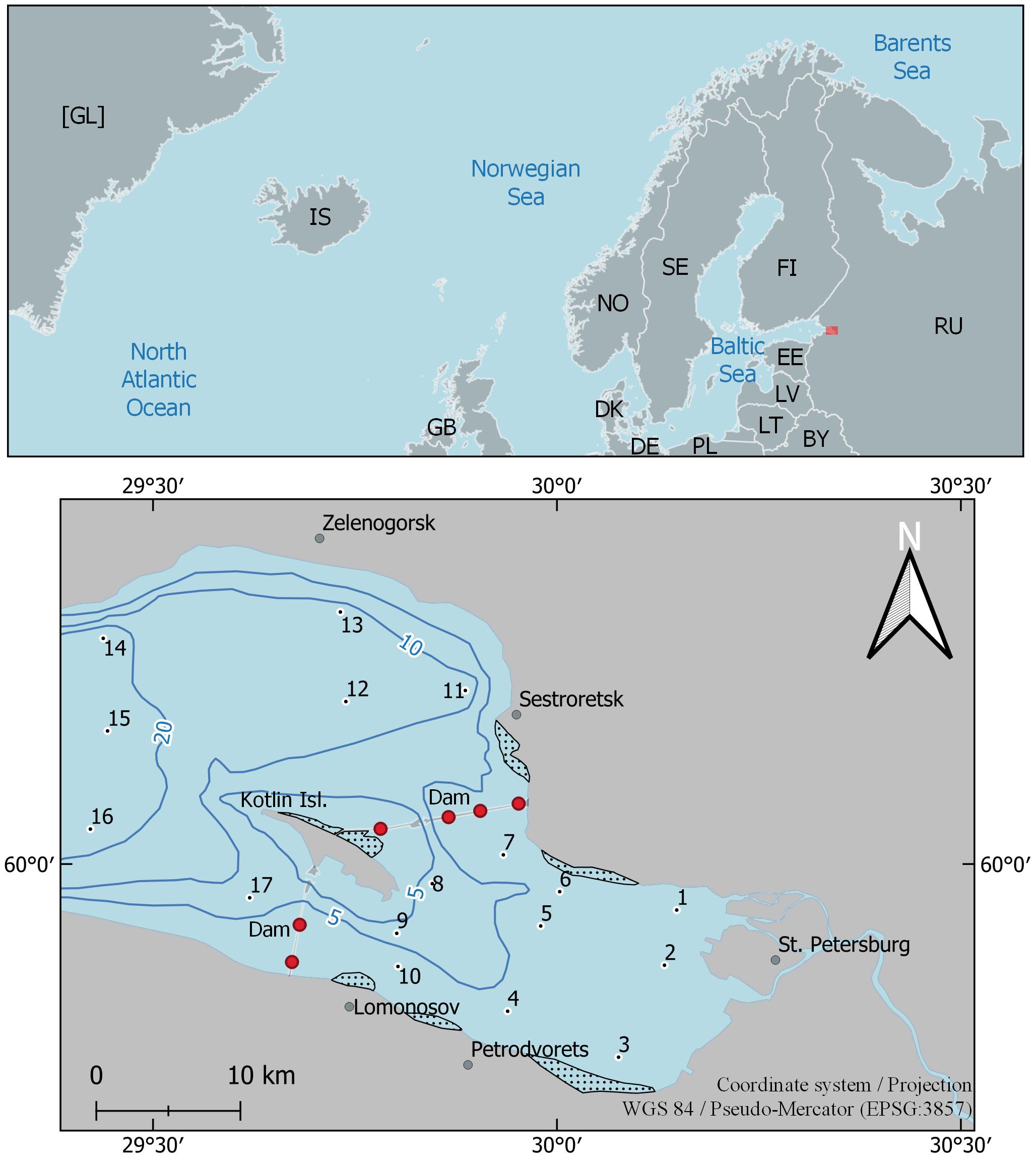
Figure 1. The upper and middle parts of the Neva Estuary with indication of sampling stations (1–17). Black lines: isobaths of 5, 10, and 20 m. Areas with dots indicate dense reeds. C1, C2—gates for vessels; D1–D6—waters gates in the St. Petersburg Flood Protection Facility. Red rectangles—the location of the Neva Estuary. Two-letter country codes are given according to ISO 3166-1 alpha-2 (International Organization for Standardization, 2020).
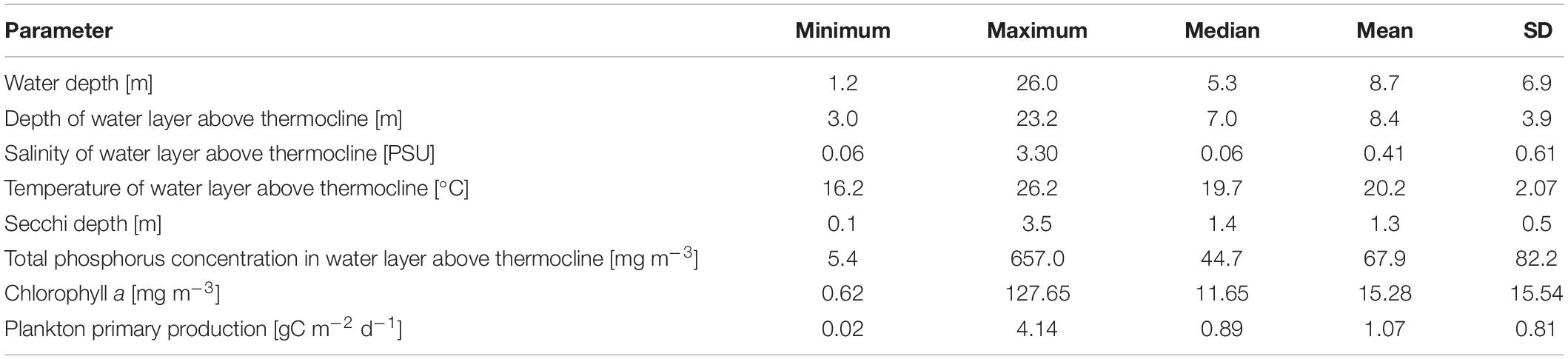
Table 1. Averaged environmental variables for the upper and middle parts of the Neva Estuary during the study period.
Phytoplankton in the Neva Estuary is represented by 174 species and forms from eight taxonomic classes (Golubkov et al., 2021). The most diverse and abundant groups of phytoplankton are cyanobacteria, green algae, and diatoms. The green algae and diatoms are dominant groups in the upper part of the estuary east of Kotlin Island. Cyanobacteria dominate in the middle part of the estuary west of Kotlin Island. Phytoplankton assemblage of the Neva Estuary and its relation to environmental factors were described in Golubkov et al. (2021).
Data and Methods
The study analyzed data on the concentration of chlorophyll a and primary production of plankton, which were determined in the course of a long-term study of the ecosystem of the Neva Estuary conducted by the Zoological Institute of the Russian Academy of Sciences. Samples were collected at 17 stations in the Neva Estuary in mid-summer in the period from late July to early August 2003–2020 (Figure 1). Chlorophyll a concentration was determined spectrophotometrically with preliminary extraction with 90% acetone (Grasshoff et al., 1999) and using a C6-multisensor platform with Cyclop-7 submersible sensor (TurnersDesigns, United States). The primary production of plankton (PP) in the water column were measured by the oxygen method of light and dark bottles (Hall et al., 2007; Vernet and Smith, 2007). Detailed description of the method, experimental design, data variability, and relation to environmental factors is given previously (Golubkov et al., 2017; Golubkov and Golubkov, 2020).
Northern Hemisphere Teleconnection Patterns
We used the values of the Arctic Oscillation (AO), North Atlantic Oscillation (NAO), East Atlantic/Western Russia (EAWR), Scandinavia (SCAND), and Polar/Eurasian (POL) indices to determine the relationships between the teleconnection patterns and indicators of phytoplankton productivity.
The AO is a large-scale regime of climate variability, also called the Northern Hemisphere annular regime. AO is a climatic pattern characterized by counterclockwise winds circulating around the Arctic at 55° north latitude (Thompson and Wallace, 1998, 2000). The NAO is based on the pressure difference at sea level between the subtropical (Azores) maximum and the subpolar minimum. The NAO index is often considered a regional manifestation of the AO index (Thompson and Wallace, 1998). NAO phases are associated with basin-scale changes in the intensity and location of the North Atlantic jet stream and storm trajectory, as well as with large-scale modulations of the normal patterns of zonal and meridional heat and moisture transport (NOAA, 2021). EAWR pattern operates in Eurasia throughout the year (Lim, 2015). The main surface temperature anomalies associated with the positive phase of the EAWR index reflect temperatures below average in large areas of western Russia and north-eastern Africa (Barnston and Livezey, 1987). The POL is closely related to the interaction between polar vortex activity in the Arctic and mid-latitude circulation over the Eurasian continent (Barnston and Livezey, 1987). The SCAND consists of a primary circulation center over Scandinavia with weaker centers of the opposite sign over Western Europe and eastern Russia/Western Mongolia. The positive phase of this model is associated with positive anomalies in the height of the isobaric surface, sometimes reflecting the main blocking anticyclones, over Scandinavia and western Russia (NOAA, 2021).
Monthly teleconnection patterns for 1950–2020 were obtained from the Climate Prediction Center (CPC) database of the National Oceanic and Atmospheric Administration (NOAA) (NOAA, 2021). Their values were averaged over the year (January–December), over the winter months (December–February), and the July values were also used. In this way, a set of fifteen index values was obtained, which were used to determine the relationship between teleconnection patterns and the concentration of chlorophyll a and plankton primary production in the Neva Estuary.
Statistical Analyses and Data Modeling
Statistical analyses were performed using R software (version 3.6.0) (R Development Core Team, 2021). For statistical analysis, data on chlorophyll a concentration and primary plankton production were averaged over 17 stations for each year. Data from 2006 to 2007 were excluded from statistical analysis because of the strong anthropogenic effect on the estuary in those years. The high concentration of phosphorus and low Secchi depth in 2006–2007 was caused by intensive dredging activity related to the construction of a new passenger port and the creation of new lands in the Neva Delta (Golubkov et al., 2008; Golubkov and Alimov, 2010). For primary production, the data for 2005 were also excluded, because in that year its values were not determined from all 17 stations. For consistency, we did not use these data in our statistical analysis. Two matrices were created. One matrix consisting of 16 rows contained chlorophyll a concentrations and climatic indices in different years. The second matrix, consisting of 15 rows, contained the values of the primary production and indices. Both matrices used for the analysis are presented in Supplementary Material.
The pairwise Pearson correlation coefficients between phytoplankton productivity indicators and climatic indices were produced using Microsoft Excel. Stepwise multiple linear regressions were performed to determine the most influential indexes affecting CHL and PP in the Neva Estuary. We have built “model.null” separately for CHL and PP and “model.full” with all indexes separately for CHL and PP. As a result, two models (null and full) was done for CHL and two for PP. Then the “step” function (direction = “both”) was used to add and remove indices from model and to find the model with the lowest Akaike Information Criterion (AIC). AIC was used as an estimator of out-of-sample prediction error and thereby relative quality of statistical models for a given set of data. The lower the value, the better for the AIC (Mangiafico, 2021). When the model with lowest AIC was found it called final.model. This procedure was done separate for CHL and PP, and two final models for CHL and PP were chosen and combinations of the most influential teleconnection patterns was found separate for CHL and PP. In the next step, we calculated the R2 for these final models. After that, we calculated the adjusted R2 (Adj R2) to avoid the error of overestimating the quality of the models, arising from the addition of each additional variable to the models. Adj R2 is a version of R2, which is calculated to take into account the number of variables in the multiple regressions model. Adj R2 is always lower than the R-squared.
We then ran an analysis of variance for the individual factors included in the final models by function “Anova” in the car R package (Fox and Weisberg, 2021) to determine which one is most important for prediction of CHL and PP in each final models. The residuals plots were checked for two final models. It showed that models were unbiased, and homoscedastic. Stepwise multiple linear regressions analysis is detailed in Mangiafico (2021). The full script of statistical analyses can be found in Supplementary Material.
Results
Analysis of Pearson’s Pairwise Correlations Between Phytoplankton Productivity Indicators and the Indices of Teleconnection Patterns
Pearson’s pairwise correlation analysis between the indicators of phytoplankton productivity in the estuary and the values of climatic indices shows the presence of statistically significant positive and negative correlation coefficients (Table 2). The concentration of chlorophyll a (CHL) positively correlated with the annual average values of the Arctic oscillation (AOy) and negatively with the values of the annual Polar/Eurasia pattern (POLy) (Table 2). The annual average values of North Atlantic oscillation (NAOy), East Atlantic/Western Russia (EAWRy), Scandinavia (SCANDy) patterns did not significantly correlate with CHL. The values of the second phytoplankton productivity indicator, the primary production of plankton (PP), did not positively correlate with any of the annual values of the indices, but negatively correlated with POLy, and the relationship with the latter was the strongest and the p-value was even < 0.01 (Table 2).
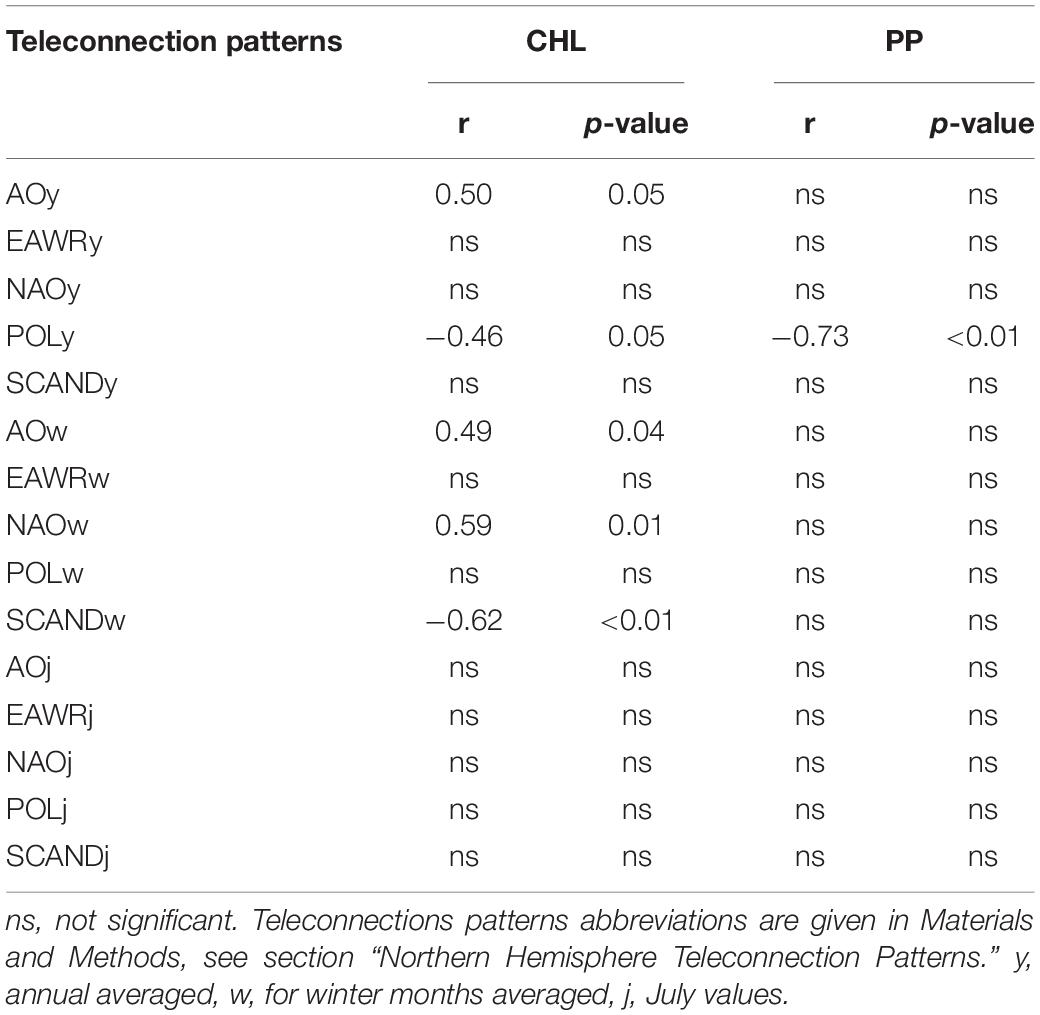
Table 2. Pearson’s correlation coefficients (r) between chlorophyll a concentration (CHL) and plankton primary production (PP) in the Neva Estuary in midsummer 2003–2005, 2008–2020, and teleconnection patterns.
Summer CHL also synchronously positively correlated with the winter value of the Arctic (AOw) and North Atlantic (NAOw) oscillations, with the strongest and most reliable correlation with NAOw (Table 2). An even stronger but negative relationship, with a p-value of < 0.01, was between CHL and the winter mean of the Scandinavia teleconnection pattern (SCANDw). Midsummer chlorophyll concentrations in the Neva Estuary were higher in years when AOw and NAOw values were higher and SCANDw values lower. Plankton primary production in midsummer did not statistically significantly correlated with any of the winter averaged indices (Table 2). Similarly, CHL and PP did not significantly correlate with any of the July indices values (Table 2).
Overall, the largest number of statistically significant correlations CHL showed with the winter averaged various indices. Therefore, AOw, NAOw, and SCANDw indices are best used to predict or reconstruct midsummer CHL values in this estuary. On the contrary, the plankton primary production correlated closely and reliably with POLy from of all the indices used.
Since chlorophyll a concentration and plankton primary production correlated differently with different climatic parameters, we analyzed the relationship between these parameters. As shown by regression analysis, these two parameters were related, the Pearson’s correlation coefficient between them was statistically significant, but not very high (Figure 2).
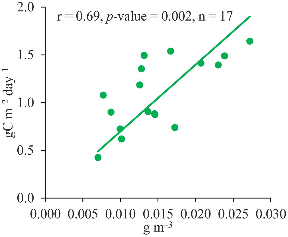
Figure 2. Relationship between midsummer chlorophyll a concentrations and plankton primary production in the Neva Estuary.
Stepwise Multiple Regression Analyses Between Phytoplankton Productivity Indicators and Teleconnection Patterns
Analysis of Pearson’s pairwise correlations showed that the concentration of chlorophyll a correlates differently with various climatic indices. On the other hand, all these teleconnection patterns are part of a single atmospheric circulation system. Therefore, it is also important to look for the relationships between the indicators of phytoplankton productivity and the set of teleconnection patterns. To achieve this goal, the method of stepwise multiple regression analysis was used. According to the graphs of the residuals of the predicted values of CHL and PP (Figure 3), both models are unbiased and homoscedastic.
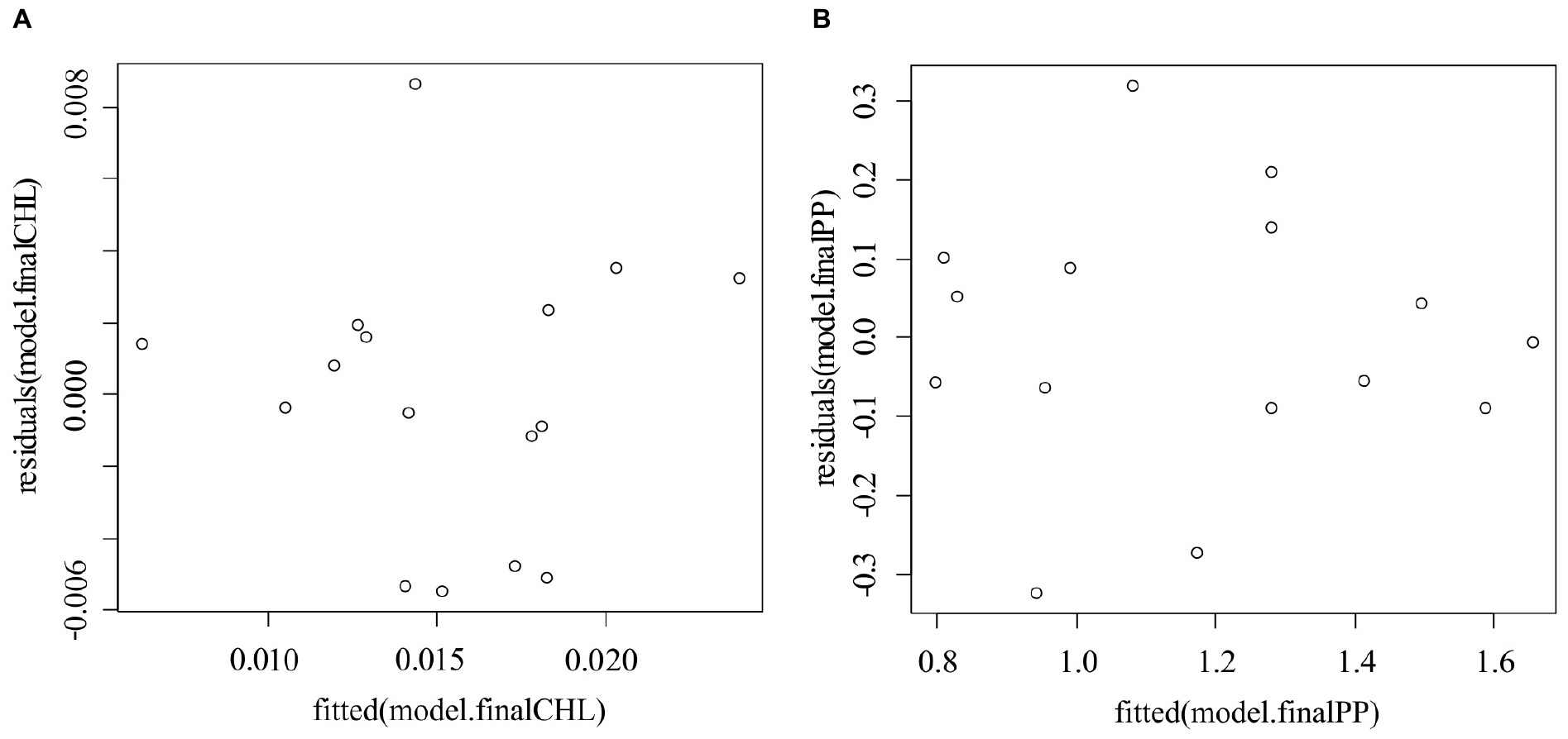
Figure 3. Plots of residuals vs. predicted values for chlorophyll a (A) and plankton primary production (B) models.
For the CHL model, the values of three of the fifteen climate indices we used, NAOw, SCANDw and POLy, were significant predictors (Table 3). The coefficient of determination was high (R2 = 0.55). However, in order to avoid the error of overestimating it, which arises as a result of adding each additional predictor to the model, we calculated the adjusted R2 (Adj R2), which also showed a high value of 0.44. This means that the resulting regression model is in good agreement with the observed CHL values. This is also evidenced by the high level of significance (p-value) of the model, 0.0196, i.e., the chances of getting a statistically significant result with this model were high. Two predictors, POLy and SCANDw, had a negative relationship with CHL values, and NAOw had a positive one. The resulting multi-regression equation describing the change in CHL values in the Neva Estuary depending on significant climatic indices is shown in Table 3.
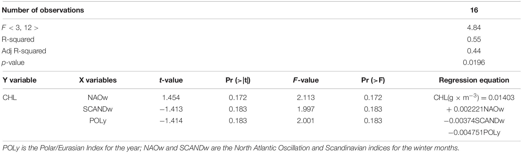
Table 3. Results of stepwise multiple regression analysis between the concentration of chlorophyll a (CHL, variable Y, predictand) and values of climatic indices (variables X, predictors).
To clarify the significance of the predictors and to find which of them most strongly affect the concentration of chlorophyll a in the estuary, we performed Student’s t-test and Fisher’s F-test. These tests showed, the addition or removal of each of these three predictors did not affect the reliability of the model (Table 3). It was important that the values of these three predictors change synchronously together.
For the primary production model, three of the fifteen predictors were also significant (Table 4). The resulting PP model had a higher linear determination coefficient (R2) and adjusted R2 than the CHL model, 0.74 and 0.67, respectively. In addition, the p-value of the PP model was an order of magnitude higher (p = 0.0014) than for the CHL model (p = 0.0196). As in the case of CHL, PP was negatively associated with the average annual values of the Polar/Eurasian pattern. Values of this pattern were the most significant predictor in the model, as shown by the t and F-tests (Table 4). As for the CHL model, the values the NAO and SCAND patterns were also additional predictors of the PP model, not for the winter months, but for July (NAOj, SCANDj), i.e., for the last month preceding the sampling period. At the same time, as t and F-tests showed, a change in each of the predictors separately affected the reliability of the model, in contrast to the model obtained for CHL. The resulting regression equation is given in Table 4.
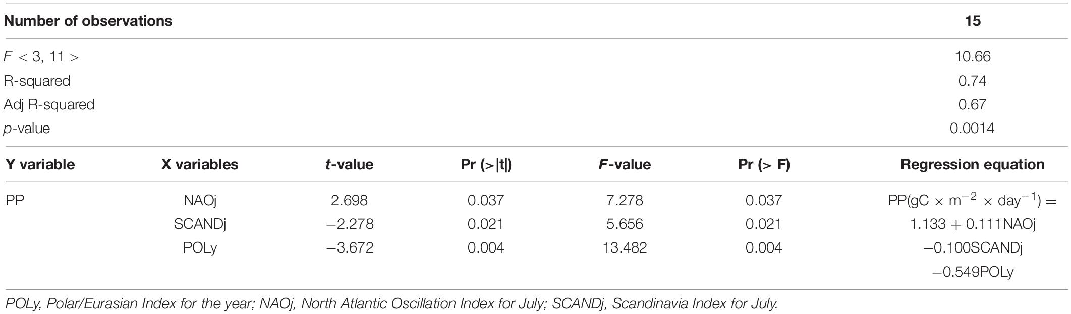
Table 4. Results of stepwise multiple regression analysis between plankton primary production (PP) (variable Y, predictand) and values of climatic indices (variables X, predictors).
Reconstruction of Chlorophyll a Concentration and Plankton Primary Production Based on Teleconnection Patterns
Using the obtained multi-regression equations and the values of the climatic indices from 1951 to 2002, we calculated the CHL and PP values for this period and plotted them on the diagrams together with the data of modern observations (Figure 4). The figures also show the calculated mean values of trophic indices for each of the obtained CHL and PP data series. The charts show CHL and PP values as positive or negative deviations relative to the calculated long-term average values for each indicator.
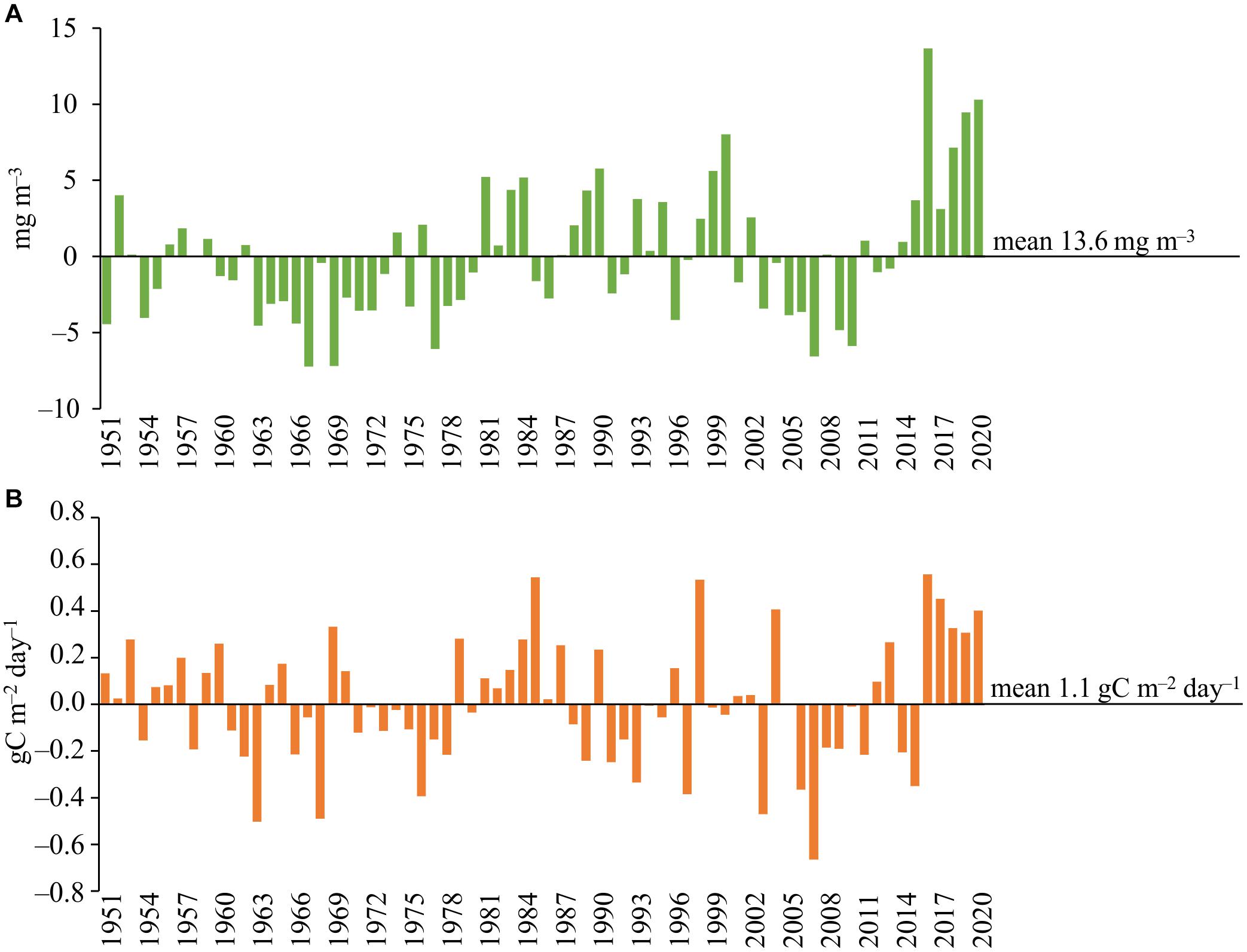
Figure 4. Concentration of chlorophyll a (A) and plankton primary production (B) in the Neva Estuary in 1951–2020. Data for 1951–2002 calculated according to the obtained multi-regression dependences, data for 2003–2020 are obtained from field observations of the authors.
The diagrams show that the values of phytoplankton productivity indicators in second part of the 2010s are significantly higher than the average long-term ones (Figure 4). The calculation using the multi-regression equation did not show such high CHL concentrations before 2000s as in second part of the 2010s, although, in some years of the 1950s, 1980s, and late 1990s, CHL could also be above average. According to our observations, CHL was noticeably below the average from 2003 to 2013, and based on the multi-regression equation, this situation could prevail throughout the second half of the twentieth century. In accordance with the teleconnection patterns, a long period with CHL values below the long-term average value could be from the late 1950s to the early 1980s, and in the 1960s, the concentration of chlorophyll a could be almost two times lower than its minimum values in the 2000s (Figure 4A).
The values of plankton primary production, like CHL, were higher than the long-term average in 2016–2020, although the same high value was in 2004 (Figure 4B). The calculations showed that similar high PP values could be observed, for example, in 1985 and 1998. Based on the obtained regression, the 1980s and most of the 1950s as a whole could be characterized by PP values higher than the long-term average (Figure 4B). As in the case of CHL, PP was below the long-term average for much of the 2000s, with a minimum in 2007. According to the values of the climatic indices, the low PP could have been in 1963, 1968, 1976, and 1997, but not as low as in 2007. A fairly long period with PP values below the long-term average could be during the entire 1970s (Figure 4B).
Discussion
Teleconnection patterns can be an important tool for investigating the impact of climate change on biological communities because of the holistic nature of the climate system (Stenseth et al., 2002). Moreover, these patterns allow to reconstruct their possible ecological characteristics in the past (Naef-Daenzer et al., 2012; Diz et al., 2018). The analysis of Pearson’s pairwise correlations between midsummer chlorophyll a concentration and plankton primary production in the Neva Estuary and the values of climatic indices showed the presence of statistically significant relationships between them (Table 2). However, these two indicators of phytoplankton productivity showed different relationships with various climatic indices. Although these two parameters are linearly related (Figure 2), the correlation coefficient between them is lower than one. The reason is that the primary production is a more physiologically mediated indicator (Andersen et al., 2006; Smith, 2007), depending not only on the concentration of pigments in algae, but also on the illumination, which changes rapidly depending on cloudy or sunny weather. Windy or calm weather can also affect the ability of algae to photosynthesize through the depth of water mixing. With weak wind mixing of the water, the algae sink to a greater depth, where the irradiation is lower (Reynolds, 1999). In other words, the concentration of chlorophyll is a more conservative indicator, which responds more slowly to changes in environmental conditions, compared to primary production. In addition, phytoplankton biomass and the concentration of chlorophyll in water depends on the sedimentation rate of phytoplankton, which differs with different phytoplankton composition (Spilling et al., 2018) and its grazing by zooplankton (Reynolds, 2006). Various groups of phytoplankton in the Neva Estuary in recent decades have shown different trends associated with fluctuations in weather conditions (Golubkov et al., 2021). As a result, the response of different characteristics of phytoplankton productivity to changes in weather conditions may differ. Therefore, when determining trends in eutrophication, it is better to use different indicators of this process including primary production (Andersen et al., 2006; Smith, 2007).
Studies of the relationship between the productivity of marine phytoplankton and the NAO pattern are the most numerous in comparison with other teleconnection patterns that we have used in our analysis (e.g., Belgrano et al., 1999; Villate et al., 2008; Boyce et al., 2010; Gladan et al., 2010). In our study, the winter NAO and SCAND indices showed statistically significant Pearson’s correlations with phytoplankton productivity (Table 2) and acted as additional predictors in the multiple regression model for chlorophyll a concentration (Table 3). In 2010s, the NAOw index was mostly in a positive phase, while the SCANDw index showed no definite trend (Figure 5). Moreover, the SCAND in the winter months have fluctuated over the past 70 years and stable positive or negative phases were not very pronounced (Figure 5B). In contrast, since the 1970s, the positive phase of the winter NAO index prevailed, and its positive values increased even more in 2012–2020 (Figure 5A).
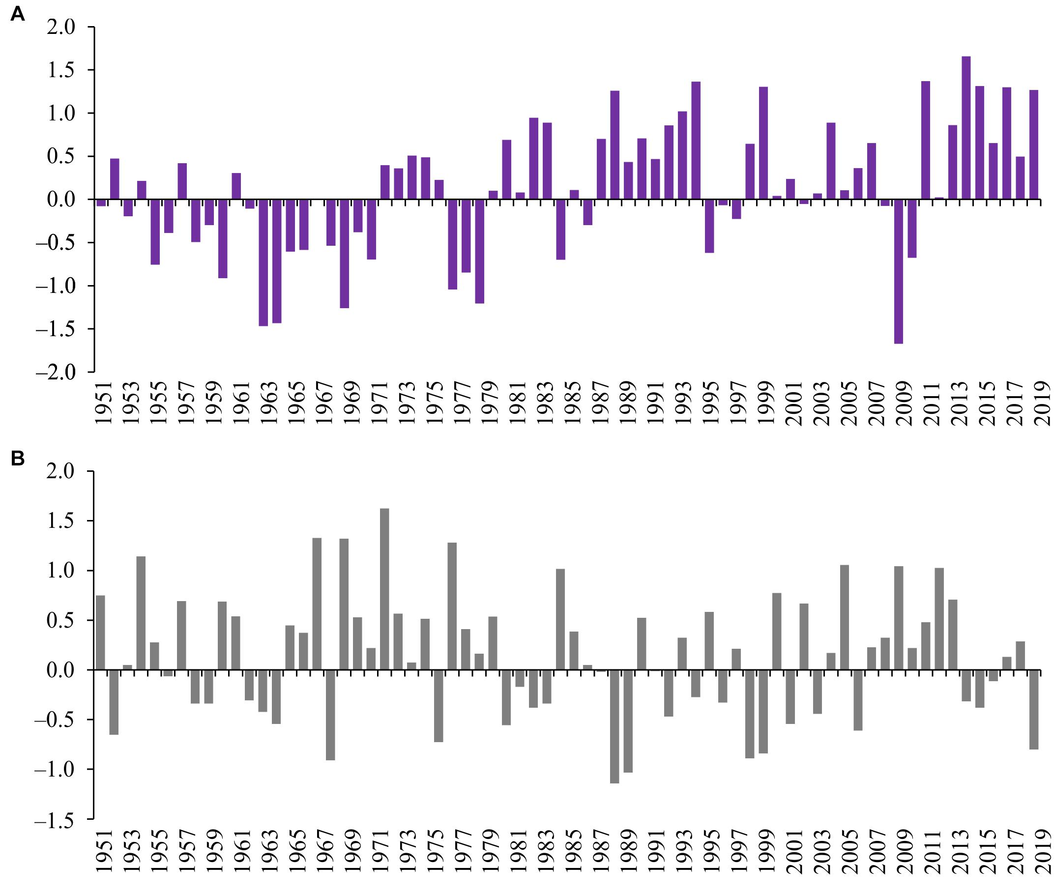
Figure 5. Winter averaged values of the North Atlantic Oscillation (A) and Scandinavia (B) indices from 1951 to 2020 (calculated according to NOAA data, 2021).
Multiple regression models obtained on the basis of 2003–2020 data allowed us to roughly reconstruct the changes in CHL and PP values in the Neva Estuary over the past 70 years, provided that their changes were controlled by the same set of factors as in the modern period. Such a reconstruction, probably, does not give a completely objective assessment of changes in these indicators in the past, since it does not take into account the influence of other environmental factors, for example, anthropogenic ones. However, it allows one to assess the state of the system before the onset of rapid climatic changes and highlight possible past periods with high or low CHL and PP values. The analysis shows that the second half of 2010s are characterized by the values of CHL and PP higher than the long-term average (Figure 4). This is especially true for CHL, as the calculation using multiple regression did not show the possibility of such high CHL values in the past. This result is consistent with the available direct measurements of chlorophyll a and plankton primary production in the Neva Estuary in the 1980s and 1990s. For example, the concentration of chlorophyll a in the middle part of the estuary was 10.57 ± 1.66 mg m–3, and the plankton primary production was 0.72 ± 0.29 gC m–2 day–1 in August 1996 (Telesh et al., 1999), which is close to their values calculated using our multi-regression equations (Figure 4). The average concentration of chlorophyll in this part of the estuary for 1983–1995 was 13.5 ± 1.04 mg m–3 (Silina, 1997), which is also close to the values according to the multi-regression equation (Figure 3).
The mechanisms of the influence of the NAO pattern on CHL and PP are very diverse. With a positive NAO phase, stronger winds are also observed in the Baltic, which leads to a stronger mixing of the water column and to the supply of additional nutrients to the surface waters (Neumann and Schernewski, 2008). In addition, with a positive NAO phase, there is an increase in the surface runoff flow from the Baltic Sea and the bottom counterflow from the North Sea (Jędrasik and Kowalewski, 2019). This can provide an influx of nutrients from the rich bottom layers to the surface waters.
A positive NAO phase and a negative SCAND phase means that warm winters with little snow cover prevail in Scandinavia and other parts of Northern Europe (Kerr, 1997; Belgrano et al., 1999; Popova, 2007). Warm winters in this region lead to an increase in the runoff of nutrients from the catchment area as a result of strong leaching of soils due to their less freezing and winter precipitation in the form of rain rather than snow (Kotta et al., 2009; Teutschbein et al., 2017; Golubkov and Golubkov, 2020). In turn, an increased runoff of nutrients can lead to an augmentation in the primary production of plankton and the concentration of chlorophyll in water. For example, warm winters led to an increase in primary production in Swedish fjords located in the Kattegat straits connecting the Baltic and North Seas; for these fjords, positive correlation coefficients were obtained between the primary production of plankton and the value of the winter NAO index (Lindahl et al., 1998; Belgrano et al., 1999). An increase in the productivity of summer phytoplankton in years with warm winters was also observed in the Neva Estuary (Golubkov and Golubkov, 2020).
In contrast to the northern regions, in the coastal part of the Adriatic Sea in southern Europe, the productivity of phytoplankton was positively correlated with NAO only in winter, but not in warmer periods, when it was negatively correlated with the values of this teleconnection pattern (Gladan et al., 2010). Unlike the Neva Estuary, which freezes in winter, photosynthesis of plankton in the Adriatic goes on all year round and is especially intense in winter, when water masses are mixed as result of strong winds during a positive NAO, as well as due to a decrease in temperature and an increase in the density of surface waters. On the contrary, dry and hot weather prevails in the Mediterranean in summer during the positive NAO phase (Hurrell et al., 2003). This increases stratification and reduces mixing of the water column and the supply of nutrients from deep layers to the surface. In spring, NAO also negatively correlated with plankton primary production, because, due to the prevalence of rainy and cloudy weather, the amount of light falling on the sea surface decreased (Gladan et al., 2010). In addition, an increase in precipitation in the European Mediterranean does not lead to an increase in the runoff of nutrients from the catchment area, because soils and river waters are rich in carbonates (Viličić et al., 2009), and their high concentrations lead to the deposition of phosphorus from solutions (Rozan et al., 2002). A negative relationship between NAO and phytoplankton productivity was also shown for the open waters of the North Atlantic, where algal productivity decreased in the positive NAO phase (Boyce et al., 2010). When NAO is positive, the region is dominated by westerly winds, which increase the temperature of the ocean surface waters and the authors hypothesize that this leads to an increase in the biomass of zooplankton, whose press reduces the biomass of phytoplankton (Boyce et al., 2010).
There are also two opposite opinions about the reasons for the current decline in phytoplankton productivity in the equatorial and subequatorial zones of the oceans. Some researchers suggest that this occurs due to the stronger stratification of oceanic waters as a result of an increase in the temperature of the upper water layer (Boyce et al., 2010; Moore et al., 2018). While others believe that modern conditions lead to a change in the strength and direction of winds affecting ocean currents and the delivery of nutrients for phytoplankton to certain zones of the oceans (Lozier et al., 2011; Whitney, 2015). These examples show that, depending on the geographic location and characteristics of the water system, as well as its catchment area, the same global patterns of atmospheric circulation can affect phytoplankton in different ways. Therefore, more research from different regions and types of waterbodies is needed to understand how modern climate change leading to temperature changes (Boyce et al., 2010; Moore et al., 2018), and the intensity and directions of atmospheric circulations (Lozier et al., 2011; Whitney, 2015) affect the productivity of phytoplankton.
The July values of the NAO and SCAND indices, which turned out to be predictors for the PP model (Table 3), are usually not used to determine the relationship between phytoplankton productivity and teleconnection patterns. Previously, it was shown that the negative SCAND phase in summer leads to lower temperatures and more precipitation in the northwest of the Russian Federation (Zveryaev and Arkhipkin, 2019). On the contrary, the positive SCAND phase in summer causes an anticyclone over Scadinavia and the appearance of an upwelling along the Polish Baltic coast due to the prevailing northeasterly winds (Bednorz et al., 2013). The SCAND pattern also strongly affects the level of the Baltic Sea, because the cyclonic center over Scandinavia, during the negative SCAND phase, enhances the western circulation, which triggers the inflow of water from the North Sea through the Danish straits into the Baltic Sea and can cause surges from the west in the Gulf of Finland (Bednorz and Tomczyk, 2021). Since the water from the Neva River flows from east to west, with a strong westerly wind, there is a surge from the open part of the Gulf of Finland and a backwater of constantly incoming river waters. This lead to the flood and increases the residence time of water in the Neva Estuary, which leads to the accumulation of phytoplankton biomass (Golubkov, 2009). Thus, weather conditions with a positive NAOj phase and a negative SCANDj phase, on the one hand, lead to an increase in the amount of precipitation and the inflow of nutrients, and, on the other hand, to the prevalence of westerly winds, which cause an increase in the water residence time in the estuary. Apparently, owing to these two mechanisms, the productivity of midsummer phytoplankton positively related with July NAO values and negatively with SCAND. This is especially true for plankton primary production, the multi-regression model of which uses NAOj and SCANDj as additional predictors (Table 4).
Pearson’s pairwise correlation analysis and stepwise multi-regression analysis showed the decisive role of the Polar/European teleconnection pattern in the phytoplankton productivity in the Neva Estuary in summer (Tables 2–4). Student’s t-test and Fisher’s F-test showed that POLy was the main predictor in multi-regression models for both indicators of phytoplankton productivity (Tables 3, 4). With negative POLy values, the concentration of chlorophyll a and planktonic primary production in the Neva Estuary increased (Tables 3, 4). Since the mid-1990s, POLy values have been mostly in the negative phase, while positive values predominated in the second half of the twentieth century (Figure 6). Therefore, it is natural that in the modern period there is an increase in the productivity of estuarine phytoplankton (Golubkov, 2009; Golubkov et al., 2017), especially in the concentration of chlorophyll a (Figure 4A) and biomasses of most phytoplankton groups (Golubkov et al., 2021).
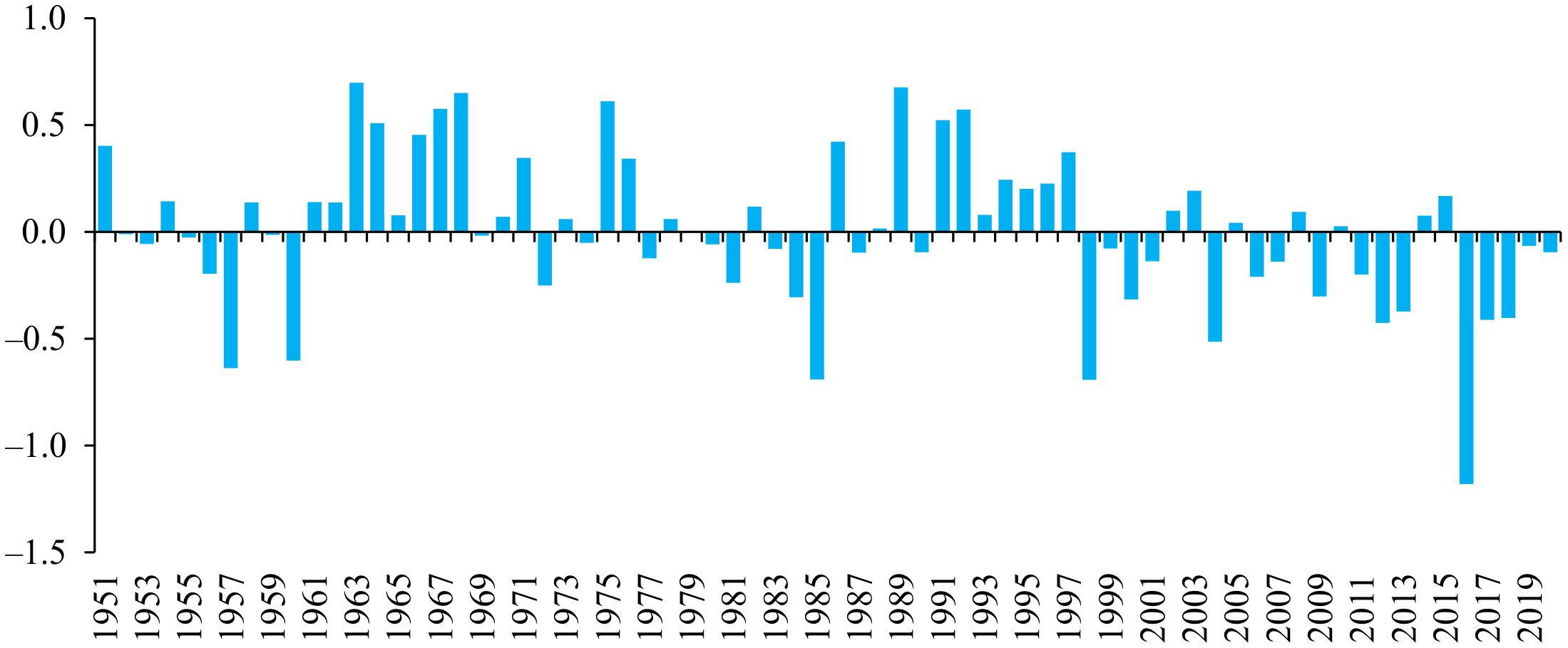
Figure 6. Averaged annual values of the Polar/Eurasian Index from 1951 to 2020 (calculated according to NOAA data, 2021).
We were unable to find any studies of the relationship between the Polar/Eurasian pattern and phytoplankton productivity indicators. However, it has been shown that the POL pattern exhibits a statistically significant negative correlation with the degree of soil moisture and a positive correlation with air temperature in June and July in northwestern European part of Russia (Zveryaev and Arkhipkin, 2019). It is also known that POL is one of the patterns that control the “Vangengeim–Girs” circulation, which forms over the Atlantic-Eurasian region and affects the westerly winds in summer (Gao et al., 2017). Strong westerly winds limit the extension of the North Polar vortex, which usually leads to its weakening and the transition of the POL pattern to a negative phase. During this phase of the POL pattern, westerly winds, as in the case of the positive phase of NAO, may lead to an extension of the water residence time in the Neva Estuary, and to an increase in the plankton primary production.
AO teleconnection pattern did not appear to be predictors of phytoplankton productivity in multi-regression analysis (Tables 3, 4). However, Pearson’s pairwise correlation analysis showed that this pattern for different periods also show statistically significant but not very high correlations with midsummer CHL (Table 2). For example, the chlorophyll a concentration in the Neva Estuary in summer correlated positively with the winter AO values. The influence of the AO teleconnection pattern on the productivity of coastal waters has not been studied very often. However, it is known that when the AO values are positive in winter, the number of cyclones arriving in the Baltic region from the North Atlantic and bringing a large amount of precipitation increases (Bednorz and Tomczyk, 2021). This, in turn, may cause an increase in phytoplankton production in the Neva Estuary (Golubkov and Golubkov, 2020). On the contrary, the negative rather than positive AO phase led to the massive development of algae in the coastal zone of the Atlantic Ocean near the Iberian Peninsula located in the southwestern part of Europe (Báez et al., 2014). There is no contradiction in these results, since it is known that the positive AO phase leads to stormy and rainy weather in northern Europe, and the negative AO phase leads to similar weather conditions in southern Europe (Thompson and Wallace, 1998).
There are even fewer studies on the effect of the EAWR teleconnection pattern on phytoplankton productivity. For example, an attempt was made to link the shift regime in the ecosystem of the Caspian Sea, which occurred in the late 1990s and mid-2000s with changes in the EAWR index, but statistically reliable results could not be obtained (Kashkooli et al., 2017). In our study, we also could not have obtained statistically significant correlations between phytoplankton productivity indicators in the Neva Estuary and EAWR teleconnection pattern (Table 2).
Our study showed that the current increase in phytoplankton productivity in the Neva Estuary is higher than it could have been in the past, provided that the regression relationships found were relevant in the past (Figure 4). This is especially true for the concentration of chlorophyll a. In the case of primary production, although the same high values could be observed earlier, but unlike in the modern period, no longer than 1 or 2 years (Figure 4B). Earlier studies have shown that ecosystem shifts occur periodically in different parts of the Baltic Sea. For example, Lindegren et al. (2012), showed a regime shift for the Kattegat straits that occurred at the turn of the 1980s and 1990s. In the mid-1980s, high primary production was observed in this part of the Baltic Sea. Then, significant changes occurred at the turn of the 1980s–1990s, and from 1992 to 2008, there was a period of low phytoplankton productivity. According to our regression models, in the mid-1980s, high plankton productivity should also have been observed in the Neva Estuary, and the 1990s and 2000s corresponded to the period of its low productivity (Figure 4). Accordingly, although these areas of the Baltic Sea are located far from each other, it is possible that the same factors could have been the trigger mechanisms for a decrease in phytoplankton productivity at that time, and such factors could be associated with atmospheric circulation. Such large-scale changes in marine ecosystems caused by atmospheric circulation have been described for the Baltic Sea (Möllmann et al., 2009) and for other marine areas (Möllmann and Diekmann, 2012; Blenckner and Niiranen, 2013).
Our analysis and the obtained multi-regression models can further make it possible to assess to what extent the changes in the ecosystem of the Neva Estuary are consistent with large-scale changes in other aquatic ecosystems that have occurred in the past. At the same time, we agree with colleagues who urge caution in such reconstructions and refine the resulting models as new evidence and data sets emerge (Murphy et al., 2020). In addition, it should be taken into account that different climatic patterns can have the most significant impact on ecosystems in certain regions. For example, according to our studies, phytoplankton productivity in the Neva Estuary located in the most northeastern part of the Baltic Sea, showed the more significant relationships with the Polar/Eurasian teleconnection pattern, which determines weather conditions in more northeastern regions of Eurasia, as compared to NAO teleconnection pattern, which mainly determines weather conditions in western Europe. Some other climatic indices also showed significant correlations with concentration of chlorophyll a and plankton primary production in the Neva Estuary. Therefore, it is important to continue research in this direction, finding out which teleconnection patterns are most informative for a particular region.
It is also worth noting that in this work we did not consider the role of the anthropogenic factor, which has a strong effect on the ecosystem of the Neva Estuary (Golubkov et al., 2019). However, unlike weather fluctuations, this factor was rather high and constant from the beginning of twentieth century and changed relatively slowly over time (Golubkov et al., 2019), making up a certain background against which changes caused by climate fluctuations took place. The study also shows that, despite all human activities transforming the biosphere, global planetary processes still have a significant impact on the environment, even in ecosystems like the Neva Estuary, which are heavily affected by anthropogenic influence. This impact should be taken into account when developing measures to protect aquatic ecosystems from eutrophication, since climate fluctuations can enhance or weaken the consequences of anthropogenic influence.
Data Availability Statement
The original contributions presented in the study are included in the article/Supplementary Material, further inquiries can be directed to the corresponding author/s.
Author Contributions
Both authors drafted, contributed to, and approved the manuscript.
Funding
The study was supported by the Ministry of Science and Higher Education of the Russian Federation (project AAAA-A19-119020690091-0).
Conflict of Interest
The authors declare that the research was conducted in the absence of any commercial or financial relationships that could be construed as a potential conflict of interest.
Publisher’s Note
All claims expressed in this article are solely those of the authors and do not necessarily represent those of their affiliated organizations, or those of the publisher, the editors and the reviewers. Any product that may be evaluated in this article, or claim that may be made by its manufacturer, is not guaranteed or endorsed by the publisher.
Acknowledgments
The authors thank the two reviewers for their constructive comments that significantly improved the early version of the manuscript.
Supplementary Material
The Supplementary Material for this article can be found online at: https://www.frontiersin.org/articles/10.3389/fmars.2021.735790/full#supplementary-material
References
Alheit, J., Möllmann, C., Dutz, J., Kornilovs, G., Loewe, P., Morholz, V., et al. (2005). Synchronous ecological regime shifts in the central Baltic and the North Sea in the late 1980s. ICES J. Mar. Sci. 62, 1205–1215. doi: 10.1016/j.icesjms.2005.04.024
Andersen, J. H., Axe, P., Backer, H., Carstensen, J., Claussen, U., Fleming-Lehtinen, V., et al. (2011). Getting the measure of eutrophication in the Baltic Sea: towards improved assessment principles and methods. Biogeochemistry 106, 137–156. doi: 10.1007/S10533-010-9508-4
Andersen, J. H., Schlüter, L., and Ærtebjerg, G. (2006). Coastal eutrophication: recent developments in definitions and implications for monitoring strategies. J. Plankton Res. 28, 621–628. doi: 10.1093/plankt/fbl001
Báez, J. C., Real, R., López-Rodas, V., Costas, E., Salvo, A. E., García-Soto, C., et al. (2014). The North Atlantic oscillation and the Arctic Oscillation favour harmful algal blooms in SW Europe. Harmful Algae 39, 121–126. doi: 10.1016/j.hal.2014.07.008
Baldwin, M. P., Dameris, M., and Shepherd, T. G. (2007). Atmosphere. How will the stratosphere affect climate change? Science 316, 1576–1577. doi: 10.1126/science.1144303
Balling, R. C. Jr., and Goodrich, G. B. (2011). Interannual variations in the local spatial autocorrelation of tropospheric temperatures. Theor. Appl. Climatol. 103, 451–457. doi: 10.1007/s00704-010-0313-8
Barnston, A. G., and Livezey, R. E. (1987). Classification, seasonality and persistence of low-frequency atmospheric circulation patterns. Mon. Weather Rev. 115, 1083–1126. doi: 10.1175/1520-04931987115<1083:CSAPOL<2.0.CO;2
Bednorz, E., and Tomczyk, A. M. (2021). Influence of macroscale and regional circulation patterns on low- and high-frequency sea level variability in the Baltic Sea. Theor. Appl. Climatol. 144, 115–125. doi: 10.1007/s00704-020-03500-0
Bednorz, E., and Wibig, J. (2008). Snow depth in eastern Europe in relation to circulation patterns. Ann. Glaciol. 48, 135–149. doi: 10.3189/172756408784700815
Bednorz, E., Półrolniczak, M., and Czernecki, B. (2013). Synoptic conditions governing upwelling along the Polish Baltic coast. Oceanologia 55, 767–785. doi: 10.5697/oc.55-4.767
Behrenfeld, M. J., O’Malley, R. T., Siegel, D. A., McClain, C. R., Sarmiento, J. L., Feldman, G. C., et al. (2006). Climate-driven trends in contemporary ocean productivity. Nature 444, 752–755. doi: 10.1038/nature05317
Bekryaev, R. V., Polyakov, I. V., and Alexeev, V. A. (2010). Role of polar amplification in long-term surface air temperature variations and modern Arctic warming. J. Climate 23, 3888–3906. doi: 10.1175/2010JCLI3297.1
Belgrano, A., Lindahl, O., and Hernroth, B. (1999). North Atlantic oscillation primary productivity and toxic phytoplankton in the Gullmar Fjord, Sweden (1985-1996). Proc. R. Soc. Lond. B 266, 425–430. doi: 10.1098/rspb.1999.0655
Blenckner, T., and Hillerbrand, H. (2002). North Atlantic oscillation signatures in aquatic and terrestrial ecosystems — a meta-analysis. Glob. Change Biol. 8, 203–212. doi: 10.1046/j.1365-2486.2002.00469.x
Blenckner, T., and Niiranen, S. (2013). “Biodiversity – marine food-web structure, stability, and regime shifts,” in Climate Vulnerability, Understanding and Addressing Threats to Essential Resources, ed. R. A. Pielke (Cambridge, MA: Academic Press), 203–212. doi: 10.1016/B978-0-12-384703-4.00423-8
Bogatov, V. V., and Fedorovskiy, A. S. (2016). Freshwater ecosystems of the southern region of the Russian far east are undergoing extreme environmental change. Knowl. Manag. Aquat. Ecosyst. 417:34. doi: 10.1051/kmae/2016021
Boyce, D. G., Lewis, M. R., and Worm, B. (2010). Global phytoplankton decline over the past century. Nature 466, 591–596.
Casanueva, A., Rodríguez-Puebla, C., Frías, M. D., and González-Reviriego, N. (2014). Variability of extreme precipitation over Europe and its relationships with teleconnection patterns. Hydrol. Earth Syst. Sci. 18, 709–725. doi: 10.5194/hess-18-709-2014
Ceglar, A., Turco, M., Toreti, A., and Doblas-Reyes, F. J. (2017). Linking crop yield anomalies to large-scale atmospheric circulation in Europe. Agric. For. Meteorol. 240–241, 35–45. doi: 10.1016/j.agrformet.2017.03.019
Damar, A., Colijn, F., Hesse, K. J., Adrianto, L., Yonvither, Fahrudin, A., et al. (2020). Phytoplankton biomass dynamics in tropical coastal waters of Jakarta Bay, Indonesia in the period between 2001 and 2019. J. Mar. Sci. Eng. 8:674. doi: 10.3390/jmse8090674
Diz, P., Hernández-Almeida, I., Bernárdez, P., Pérez-Arlucea, M., and Hall, I. R. (2018). Ocean and atmosphere teleconnections modulate east tropical Pacific productivity at late to middle Pleistocene terminations. Earth Planet. Sci. Lett. 493, 82–91. doi: 10.1016/j.epsl.2018.04.024
Doney, S. C., Ruckelshaus, M., Duffy, J. E., Barry, J. P., Chan, F., English, C. A., et al. (2012). Climate change impacts on marine ecosystems. Annu. Rev. Mar. Sci. 4, 11–37. doi: 10.1146/annurev-marine-041911-111611
Filatov, N. N., Viruchalkina, T. Y., Dianskiya, N. A., Nazarovaa, L. E., and Sinukovich, V. N. (2016). Intrasecular variability in the level of the largest lakes of Russia. Dokl. Earth Sci. 467, 393–397. doi: 10.1134/S1028334X16040097
Fox, J., and Weisberg, S. (2021). Car: Companion to Applied Regression. Available online at: https://cran.r-project.org/web/packages/car/index.html (accessed on July 1, 2021).
Friedland, R., Neumann, T., and Schernewski, G. (2012). Climate change and the Baltic Sea action plan: model simulations on the future of the western Baltic Sea. J. Mar. Syst. 105–108, 175–186. doi: 10.1016/j.jmarsys.2012.08.002
Gao, T., Yu, J., and Paek, H. (2017). Impacts of four northern-hemisphere teleconnection patterns on atmospheric circulations over Eurasia and the Pacific. Theor. Appl. Climatol. 129, 815–831. doi: 10.1007/s00704-016-1801-2
Girjatowicz, J. P., and Małgorzata, Ś (2019). Effects of atmospheric circulation on water temperature along the southern Baltic Sea coast. Oceanologia 61, 38–49. doi: 10.1016/j.oceano.2018.06.002
Gladan, ŽN., Marasović, I., Grbec, B., Skejić, S., Bužančić, M., Kušpilić, G., et al. (2010). Inter-decadal variability in phytoplankton community in the Middle Adriatic (Kaštela Bay) in relation to the North Atlantic oscillation. Estuar. Coast. 33, 376–383. doi: 10.1007/s12237-009-9223-3
Golubkov, M. S. (2009). Phytoplankton primary production in the Neva Estuary at the turn of the 21st century. Inland Water Biol. 2, 312–318. doi: 10.1134/S199508290904004X
Golubkov, M. S., Golubkov, S. M., and Umnova, L. P. (2008). “Role of sedimentation and resuspension of particulate matter in fluctuations of trophic status of the Neva Estuary,” in Proceedings of IEEE/OES US/EU-Baltic International Symposium, 27–29 May 2008, (Tallinn). doi: 10.1109/BALTIC.2008.4625559
Golubkov, M. S., Nikulina, V. N., and Golubkov, S. M. (2021). Species-level associations of phytoplankton with environmental variability in the Neva Estuary (Baltic Sea). Oceanologia 63, 149–162. doi: 10.1016/j.oceano.2020.11.002
Golubkov, M., and Golubkov, S. (2020). Eutrophication in the Neva Estuary (Baltic Sea): response to temperature and precipitation patterns. Mar. Freshw. Res. 71, 583–595. doi: 10.1071/MF18422
Golubkov, S. M. (2021). Effect of climatic fluctuations on the structure and functioning of ecosystems of continental water bodies. Contemp. Probl. Ecol. 14, 1–10. doi: 10.1134/S1995425521010030
Golubkov, S. M., Golubkov, M. S., and Tiunov, A. V. (2019). Anthropogenic carbon as a basal resource in the benthic food webs in the Neva Estuary (Baltic Sea). Mar. Pollut. Bull. 146, 190–200. doi: 10.1016/j.marpolbul.2019.06.037
Golubkov, S., and Alimov, A. (2010). Ecosystem changes in the Neva Estuary (Baltic Sea): natural dynamics or response to anthropogenic impacts? Mar. Pollut. Bull. 61, 198–204. doi: 10.1016/J.MARPOLBUL.2010.02.014
Golubkov, S., Golubkov, M., Tiunov, A., and Nikulina, L. (2017). Long-term changes in primary production and mineralization of organic matter in the Neva Estuary (Baltic Sea). J. Mar. Syst. 171, 73–80. doi: 10.1016/j.jmarsys.2016.12.009
Grasshoff, K., Ehrhardt, M., and Kremling, K. (1999). Methods of Seawater Analysis, 3rd, Completely Rev. and Extended Edn. New York: Wiley-VCH.
Greaves, B. L., Davidson, A. T., Fraser, A. D., McKinlay, J. P., Martin, A., McMinn, A., et al. (2020). The southern annular mode (SAM) influences phytoplankton communities in the seasonal ice zone of the Southern Ocean. Biogeosciences 17, 3815–3835. doi: 10.5194/bg-17-3815-2020
Gubelit, Y. I (2015). Climatic impact on community of filamentous macroalgae in the Neva estuary (eastern Baltic Sea). Mar. Pollut. Bull. 91, 166–172. doi: 10.1016/j.marpolbul.2014.12.009
Hall, R. O. Jr., Thomas, S., and Gaiser, E. E. (2007). “Measuring freshwater primary production and respiration,” in Principles and Standards for Measuring Primary Production, eds T. J. Fahey and A. K. Knapp (Oxford: Oxford University Press), 175–203. doi: 10.1093/acprof:oso/9780195168662.003.0010
Heisler, J., Glibert, P. M., Burkholder, J. M., Anderson, D. M., Cochlan, W., Dennison, W. C., et al. (2008). Eutrophication and harmful algal blooms: a scientific consensus. Harmful Algae 8, 3–13. doi: 10.1016/j.hal.2008.08.006
Holt, J., Schrum, C., Cannaby, H., Daewel, U., Allen, I., Artioli, Y., et al. (2016). Potential impacts of climate change on the primary production of regional seas: a comparative analysis of five European seas. Prog. Oceanogr. 140, 91–115. doi: 10.1016/j.pocean.2015.11.004
Hurrell, J. W., Kushnir, Y., Ottersen, G., and Visbeck, M. (2003). “An overview of the North Atlantic oscillation,” in The North Atlantic Oscillation, Climatic Significance and Environmental Impact, Vol. 134, eds J. W. Hurrell, Y. Kushnir, G. Ottersen, and M. Visbeck (Washington, DC: American Geophysical Union), 1–35. doi: 10.1029/134GM01
International Organization for Standardization (ISO) (2020). Country Codes – ISO 3166. Available online at: https://www.iso.org/iso-3166-country-codes.html (accessed on July 1, 2021).
Ionita, M. (2014). The impact of the East Atlantic/Western Russia pattern on the hydroclimatology of Europe from Mid-Winter to late spring. Climate 2, 296–309. doi: 10.3390/cli2040296
Jędrasik, J., and Kowalewski, M. (2019). Mean annual and seasonal circulation patterns and long-term variability of currents in the Baltic Sea. J. Mar. Syst. 193, 1–26. doi: 10.1016/j.jmarsys.2018.12.011
Jevrejeva, S., Moore, J. C., and Grinsted, A. (2003). Influence of the Arctic oscillation and El Niño-Southern oscillation (ENSO) on ice conditions in the Baltic Sea: the wavelet approach. J. Geophys. Res. Atmos. 108:4677. doi: 10.1029/2003JD003417
Kashkooli, O. B., Gröger, J., and Núñez-Riboni, I. (2017). Qualitative assessment of climate-driven ecological shifts in the Caspian Sea. PLoS One 12:e0176892. doi: 10.1371/journal.pone.0176892
Kerr, R. A. (1997). A new driver for the Altlantic’s moods and European weather? Science 275, 754–755. doi: 10.1126/science.288.5473.1984
Kotta, J., Kotta, I., Simm, M., and Põllupüü, M. (2009). Separate and interactive effects of eutrophication and climate variables on the ecosystem elements of the Gulf of Riga. Estuar. Coast. Shelf Sci. 84, 509–518. doi: 10.1016/j.ecss.2009.07.014
Kottek, M., Grieser, J., Beck, C., Rudolf, B., and Rubel, F. (2006). World Map of the Köppen-Geiger climate classification updated. Meteorol. Z. 15, 259–263. doi: 10.1127/0941-2948/2006/0130
Krichak, S. O., and Alpert, P. (2005). Decadal trends in the east Atlantic–west Russia pattern and Mediterranean precipitation. Int. J. Climatol. 25, 183–192. doi: 10.1002/joc.1124
Le, C., Wu, S., Hu, C., Beck, M. W., and Yang, X. (2019). Phytoplankton decline in the eastern North Pacific transition zone associated with atmospheric blocking. Glob. Change Biol. 25, 3485–3493. doi: 10.1111/gcb.14737
Lim, Y.-K. (2015). The East Atlantic/West Russia (EA/WR) teleconnection in the North Atlantic: climate impact and relation to Rossby wave propagation. Clim. Dyn. 44, 3211–3222. doi: 10.1007/s00382-014-2381-4
Lindahl, O., Belgrano, A., Davidsson, L., and Hernroth, B. (1998). Primary production, climatic oscillations, and physico-chemical processes: the Gullmar Fjord time-series data set (1985–1996). ICES J. Mar. Sci. 55, 723–729. doi: 10.1006/jmsc.1998.0379
Lindegren, M., Blenckner, T., and Stenseth, N. C. (2012). Nutrient reduction and climate change cause a potential shift from pelagic to benthic pathways in a eutrophic marine ecosystem. Glob. Change Biol. 18, 3491–3503. doi: 10.1111/j.1365-2486.2012.02799.x
Lozier, M. S., Dave, A. C., Palter, J. B., Gerber, L. M., and Barber, R. T. (2011). On the relationship between stratification and primary productivity in the North Atlantic. Geophys. Res. Lett. 38:L18609. doi: 10.1029/2011GL049414
Luterbacher, J., Schmutz, C., Gyalistras, D., Xoplaki, E., and Wanner, H. (1999). Reconstruction of monthly NAO and EU indices back to AD 1675. Geophys. Res. Lett. 26, 2745–2748. doi: 10.1029/1999GL900576
Luterbacher, J., Xoplaki, E., Dietrich, D., Jones, P. D., Davies, T. D., Portis, D., et al. (2004). Extending North Atlantic oscillation reconstructions back to 1500. Atmos. Sci. Lett. 2, 114–124. doi: 10.1006/asle.2002.0047
Mangiafico, S. S. (2021). An R Companion for the Handbook of Biological Statistics. Available online at: https://rcompanion.org/rcompanion/e_05.html (accessed on July 1, 2021).
Maximov, A. A., Berezina, N. A., and Maximova, O. B. (2021). Interannual changes in benthic biomass under climate-induced variations in productivity of a small northern lake. Fundam. Appl. Limnol. 194, 187–199. doi: 10.1127/fal/2020/1291
Meier, H. E. M., Hordoir, R., Andersson, H. C., Dieterich, C., Eilola, K., Gustafsson, B. G., et al. (2012). Modeling the combined impact of changing climate and changing nutrient loads on the Baltic Sea environment in an ensemble of transient simulations for 1961–2099. Clim. Dynam. 39, 2421–2441. doi: 10.1007/s00382-012-1339-7
Meteoblue (2021). Climate Zones. Available online at: https://content.meteoblue.com/en/meteoscool/general-climate-zones (Accessed on June 29, 2021).
Möllmann, C., and Diekmann, R. (2012). “Marine ecosystem regime shifts induced by climate and overfishing: a review for the northern hemisphere,” in Advances in Ecological Research volume 47, Global Change in Multispecies Systems, Part 2, eds G. Woodward, U. Jacob, and E. J. O’Gorman (Cambridge, MA: Academic Press), 303–347. doi: 10.1016/B978-0-12-398315-2.00004-1
Möllmann, C., Diekmann, R., Müller-Karulis, B., Kornilovs, G., Plikshs, M., and Axe, P. (2009). Reorganization of a large marine ecosystem due to atmospheric and anthropogenic pressure: a discontinuous regime shift in the central Baltic Sea. Glob. Change Biol. 15, 1377–1393. doi: 10.1111/j.1365-2486.2008.01814.x
Moore, J. K., Fu, W., Primeau, F., Britten, G. L., Lindsay, K., Long, M., et al. (2018). Sustained climate warming drives declining marine biological productivity. Science 359, 1139–1143. doi: 10.1126/science.aao6379
Murphy, C., Wilby, R. L., Matthews, T. K. R., Thorne, P., Broderick, C., Fealy, R., et al. (2020). Multi-century trends to wetter winters and drier summers in the England and Wales precipitation series explained by observational and sampling bias in early records. Int. J. Climatol. 40, 610–619. doi: 10.1002/joc.6208
Naef-Daenzer, B., Luterbacher, J., Nuber, M., Rutishauser, T., and Winkel, W. (2012). Cascading climate effects and related ecological consequences during past centuries. Clim. Past 8, 1527–1540. doi: 10.5194/cp-8-1527-2012
Neumann, T., and Schernewski, G. (2008). Eutrophication in the Baltic Sea and shifts in nitrogen fixation analyzed with a 3D ecosystem model. J. Mar. Syst. 74, 592–602. doi: 10.1016/j.jmarsys.2008.05.003
NOAA (2021). Northern Hemisphere Teleconnection Patterns. Available online at: https://www.cpc.ncep.noaa.gov/data/teledoc/telecontents.shtml (accessed on July 1, 2021).
Plewa, K., Perz, A., and Wrzesiński, D. (2019). Links between teleconnection patterns and water level regime of selected polish lakes. Water 11:1330. doi: 10.3390/w11071330
Popova, V. (2007). Winter snow depth variability over northern Eurasia in relation to recent atmospheric circulation changes. Int. J. Climatol. 27, 1721–1733. doi: 10.1002/joc.1489
Ptak, M., Tomczyk, A., and Wrzesiński, D. (2018). Effect of teleconnection patterns on changes in water temperature in Polish lakes. Atmosphere 9:66. doi: 10.3390/atmos9020066
R Development Core Team (2021). The R Project for Statistical Computing (Version 3.6.0). Available online at: https://www.r-project.org (accessed on July 1, 2021).
Reynolds, C. S. (1999). “With or against the grain: responses of phytoplankton to pelagic variability,” in Aquatic Life Cycle Strategies: Survival in a Variable Environment, eds M. Whitfield, J. Matthews, and C. Reynolds (Plymouth: The Marine Biological Association of the United Kingdom), 15–45.
Reynolds, C. S. (2006). Ecology of Phytoplankton. Cambridge: Cambridge University Press. doi: 10.1017/CBO9780511542145
Rozan, T. F., Taillefert, M., Trouwborst, R. E., Glazer, B. T., Ma, S., Herszage, J., et al. (2002). Iron-sulfur-phosphorus cycling in the sediments of shallow coastal bay: implication for sediments nutrient release and benthic macroalgal blooms. Limnol. Oceanogr. 47, 1346–1354. doi: 10.4319/lo.2002.47.5.1346
Ryabchuk, D., Zhamoida, V., Orlova, M., Sergeev, A., Bublichenko, J., Bublichenko, A., et al. (2017). “Neva Bay: a technogenic lagoon of the eastern Gulf of Finland (Baltic Sea),” in The Diversity of Russian Estuaries and Lagoons Exposed to Human Influence, ed. R. Kosyan (Cham: Springer International Publishing), 191–221. doi: 10.1007/978-3-319-43392-9
Schaefer, K., Denning, A. S., and Leonard, O. (2004). The winter Arctic oscillation and the timing of snowmelt in Europe. Geophys. Res. Lett. 31:L22205. doi: 10.1029/2004GL021035
Sharov, A. N., Berezina, N. A., Nazarova, L. E., Poliakova, T. N., and Chekryzheva, T. A. (2014). Links between biota and climate-related variables in the Baltic region using Lake Onega as an example. Oceanologia 56, 291–306. doi: 10.5697/oc.56-2.291
Silina, N. I. (1997). “Content of photosynthetic pigments of suspended organic matter and seston in plankton in ecosystem models,” in Assessment of the Current State of the Gulf of Finland. Part 2. Hydrometeorological, Hydrochemical, Hydrobiological, Geological Conditions and Water Dynamics in the Gulf of Finland, eds I. N. Davidan and O. P. Savchuk (Saint-Petersburg: Hydrometeoizdat), 365–375. (In Russian).
Smith, V. H. (2007). Using primary productivity as an index of coastal eutrophication: the units of measurement matter. J. Plankton Res. 29, 1–6. doi: 10.1093/plankt/fbl061
Spilling, K., Olli, K., Lehtoranta, J., Kremp, A., Tedesco, L., Tamelander, T., et al. (2018). Shifting diatom—dinoflagellate dominance during spring bloom in the Baltic Sea and its potential effects on biogeochemical cycling. Front. Mar. Sci. 5:327. doi: 10.3389/fmars.2018.00327
Stenseth, N. C., Mysterud, A., Ottersen, G., Hurrell, J. W., Chan, K.-S., and Lima, M. (2002). Ecological effects of climate fluctuations. Science 297, 1292–1296. doi: 10.1126/SCIENCE.1071281
Straile, D., and Adrian, R. (2000). The North Atlantic oscillation and plankton dynamics in two European lakes: two variations on a general theme. Glob. Change Biol. 6, 663–670. doi: 10.1046/j.1365-2486.2000.00350.x
Straile, D., Livingstone, D. M., Weyhenmeyer, G. A., and George, D. G. (2003). The response of freshwater ecosystems to climate variability associated with the North Atlantic oscillation. Geophys. Monogr. Series 134, 263–279. doi: 10.1029/134GM12
Telesh, I. V., Alimov, A. F., Golubkov, S. M., Nikulina, V. N., and Panov, V. E. (1999). Response of aquatic communities to anthropogenic stress: a comparative study of Neva Bay and the eastern Gulf of Finland. Hydrobiologia 393, 95–105. doi: 10.1023/A:1003578823446
Teutschbein, C., Sponseller, R. A., Grabs, T., Blackburn, M., Boyer, E. W., Hytteborn, J. K., et al. (2017). Future riverine inorganic nitrogen load to the Baltic Sea from Sweden: an ensemble approach to assessing climate change effects. Global Biogeochem. Cycles 31, 1674–1701. doi: 10.1002/2016GB005598
Thompson, D. W. J., and Wallace, J. M. (1998). The Arctic oscillation signature in the wintertime geopotential height and temperature fields. Geophys. Res. Lett. 25, 1297–1300. doi: 10.1029/98GL00950
Thompson, D. W. J., and Wallace, J. M. (2000). Annular modes in the extratropical circulation. Part I. Month to month variability. J. Climate 13, 1000–1016. doi: 10.1175/1520-04422000013<1000:AMITEC<2.0.CO;2
Trigo, R. M., Osborn, T. J., and Corte-Real, J. M. (2002). The North Atlantic oscillation influence on Europe: climate impacts and associated physical mechanisms. Clim. Res. 20, 9–17. doi: 10.3354/cr020009
Trigo, R. M., Pozo-Vázquez, D., Osborn, T. J., Castro-Díez, Y., Gámiz-Fortis, S., and Esteban-Parra, M. J. (2004). North Atlantic oscillation influence on precipitation, river flow and water resources in the Iberian Peninsula. Int. J. Climatol. 24, 925–944. doi: 10.1002/joc.1048
Uvo, C. B., Foster, K., and Olsson, J. (2021). The spatio-temporal influence of atmospheric teleconnection patterns on hydrology in Sweden. J. Hydrol. 34:100782. doi: 10.1016/j.ejrh.2021.100782
Vernet, M., and Smith, R. C. (2007). “Measuring and modeling primary production in marine pelagic ecosystems,” in Principles and Standards for Measuring Primary Production, eds T. J. Fahey and A. K. Knapp (Oxford: Oxford University Press), 142–174. doi: 10.1093/acprof:oso/9780195168662.003.0009
Viličić, D., Djakovac, T., Burić, Z., and Bosak, S. (2009). Composition and annual cycle of phytoplankton assemblages in the northeastern Adriatic Sea. Bot. Mar. 52, 291–305. doi: 10.1515/BOT.2009.004
Villate, F., Aravena, G., Iriarte, A., and Uriarte, I. (2008). Axial variability in the relationship of chlorophyll a with climatic factors and the North Atlantic oscillation in a Basque coast estuary, Bay of Biscay (1997–2006). J. Plankton Res. 30, 1041–1049. doi: 10.1093/plankt/fbn056
Wang, D., Wang, C., Yang, X., and Lu, J. (2005). Winter Northern Hemisphere surface air temperature variability associated with the Arctic oscillation and North Atlantic oscillation. Geophys. Res. Lett. 32:L16706. doi: 10.1029/2005GL022952
Weyhenmeyer, G. A. (2008). Rates of change in physical and chemical lake variables – are they comparable between large and small lakes? Hydrobiologia 599, 105–110. doi: 10.1007/s10750-007-9193-z
Whitney, F. A. (2015). Anomalous winter winds decrease 2014 transition zone productivity in the NE Pacific. Geophys. Res. Lett. 42, 428–431.
Yao, Y., and Luo, D. H. (2018). An asymmetric spatiotemporal connection between the Euro-Atlantic blocking within the NAO life cycle and European climates. Adv. Atmos. Sci. 35, 796–812. doi: 10.1007/s00376-017-7128-9
Keywords: phytoplankton, primary production, chlorophyll, eutrophication indicators, climatic fluctuation, climate indices, atmospheric circulation, NAO
Citation: Golubkov M and Golubkov S (2021) Relationships Between Northern Hemisphere Teleconnection Patterns and Phytoplankton Productivity in the Neva Estuary (Northeastern Baltic Sea). Front. Mar. Sci. 8:735790. doi: 10.3389/fmars.2021.735790
Received: 03 July 2021; Accepted: 26 August 2021;
Published: 21 September 2021.
Edited by:
Bernardo Antonio Perez Da Gama, Fluminense Federal University, BrazilReviewed by:
Alberto Basset, University of Salento, ItalyNatalya Mineeva, Institute of Biology of Inland Waters, Russian Academy of Sciences, Russia
Copyright © 2021 Golubkov and Golubkov. This is an open-access article distributed under the terms of the Creative Commons Attribution License (CC BY). The use, distribution or reproduction in other forums is permitted, provided the original author(s) and the copyright owner(s) are credited and that the original publication in this journal is cited, in accordance with accepted academic practice. No use, distribution or reproduction is permitted which does not comply with these terms.
*Correspondence: Mikhail Golubkov, Z29sdWJrb3ZfbXNAbWFpbC5ydQ==