Seagrass Depth Distribution Mirrors Coastal Development in the Mexican Caribbean – An Automated Analysis of 800 Satellite Images

The seagrass Thalassia testudinum is the dominant habitat-builder in coastal reef lagoons of the Caribbean, and provides vital ecosystem services including coastal protection and carbon storage. We used a remote sensing methodology to map T. testudinum canopies over 400 km of coastline of the eastern Yucatán Peninsula, comparing the depth distribution of canopy density, in terms of leaf area index (LAI), to a previously established ecological model of depth and LAI for this species in oligotrophic conditions. The full archive of Sentinel-2 imagery from 2016 to 2020 was applied in an automated model inversion method to simultaneously estimate depth and LAI, covering ∼900 km² of lagoon with approximately 800 images. Data redundancy allowed for statistical tests of change detection. Achieved accuracy was sufficient for the objectives: LAI estimates compared to field data had mean absolute error of 0.59, systematic error of 0.04 and r² > 0.67 over a range of 0–5. Bathymetry compared to 46,000 ICESat-2 data points had a mean absolute error of 1 m, systematic error less than 0.5 m, and r² > 0.88 over a range of 0–15 m. The estimated total area of seagrass canopy was consistent with previously published estimates of ∼580 km², but dense canopies (LAI > 3), which are the primary contributors to below-ground carbon storage, comprise only ∼40 km². Within the year-to-year variation there was no change in overall seagrass abundance 2017–2020, but localised statistically significant (p < 0.01) patches of canopy extension and retraction occurred. 2018 and 2019 were affected by beaching of pelagic Sargassum and dispersion as organic matter into the lagoon. The multi-year analysis enabled excluding this influence and provided an estimate of its extent along the coast. Finally, the distribution of LAI with depth was consistent with the ecological model and showed a gradient from north to south which mirrored a well-established gradient in anthropogenic pressure due to touristic development. Denser canopies were more abundant in developed areas, the expected growth response to nutrient enrichment. This increase in canopy density may be a useful early bio-indicator of environmental eutrophication, detectable by remote sensing before habitat deterioration is observed.

Introduction

Seagrass beds worldwide are of significant environmental and economic importance (Costanza et al., 1997). These highly productive coastal ecosystems (Duarte and Chiscano, 1999) provide numerous services including coastal protection, fisheries support, trapping and stabilization of sediments, nutrient biogeochemical cycling, and carbon storage (Fonesca and Cahalan, 1992; Gacia et al., 1999; Agawin and Duarte, 2002; Duarte et al., 2005; Gillanders, 2006; Romero et al., 2006; Kennedy et al., 2010; Fourqurean et al., 2012; Enríquez et al., 2019). Monitoring the state of these ecosystems is therefore an important activity for management and policy guidance, particularly under environmental stressors such as coastal development and eutrophication (Waycott et al., 2009; Grech et al., 2011). In addition, seagrass habitats may be useful environmental bioindicators (Orth et al., 2006). As seagrasses are faster growers than corals, the effects of eutrophication or other stressors may be apparent earlier, and at larger scales, than in the associated coral reefs. However, studies have yet to conclusively demonstrate this link (van Tussenbroek et al., 2014; Cortés et al., 2019).

The response at the individual plant or canopy level to trophic changes involves many factors, which may not directly represent trends at the ecosystem level (Cabaço et al., 2013). In the Caribbean, long-term in situ monitoring of tropical seagrass meadows by the CARICOMP initiative (CARICOMP, 1994; Cortés et al., 2019) has documented a large variation in seagrass productivity and biomass across the wide Caribbean, but only a weak association with nutrient enrichment (van Tussenbroek, 2011; van Tussenbroek et al., 2014) or with the physicochemical provinces (PECS) defined by Chollett et al. (2012). A recent study of meadows of Thalassia testudinum, the climax species in the Caribbean, indicates the relevance of light and canopy self-shading as an explanatory mechanism for gradients in plant morphology and biomass with depth (Enríquez et al., 2019). Hence, when comparing areas with contrasting depths, the impact of factors such as eutrophication may be masked by bio-physical constraints in canopy structure and light capture. This may explain why no clear trends associated with eutrophication or environmental deterioration have been identified in previous long-term studies. In the Mediterranean species Posidonia oceanica, a species with leaf area index (LAI) values up to 12–15 (Olesen et al., 2002), depth has been shown to be a complicating factor for many bio-indicators including canopy cover (Martínez-Crego et al., 2008).

Leaf area index (LAI) is a useful metric of canopy density, being the total single-sided leaf area divided by the substrate area. Compared to above-ground biomass, LAI is more directly related to light collection, leaf productivity and self-shading in the canopy, and also to the canopy reflectance as detectable by satellite remote sensing (Hedley and Enríquez, 2010; Hedley et al., 2014). Using data from 2004 of Thalassia testudinum in a reef lagoonal system under oligotrophic conditions, Enríquez et al. (2019) demonstrated a negative exponential relationship between depth and LAI, for LAI values up to 5. In addition, the capacity for carbon storage was shown to substantially reduce with depth, and was only significant under shallow dense canopies, e.g., LAI greater than 3 in depths less than 2 m. The conditions the model was developed in were water column concentrations of dissolved inorganic nitrogen (DIN) and phosphorus (DIP) below nutrient thresholds of 1 and 0.1 μM, respectively (Lapointe, 1997). For comparison, the Mexican CONAGUA (Comisión Nacional del Agua) follow the water quality guidelines of the U.S. Environmental Protection Agency (2017) for environmental assessments in coral reef systems, as well as those suggested by Bricker et al. (1999), and, according to these references, “good” quality water conditions are DIN and DIP below 3.57 and 0.16 μM, respectively, whereas “poor” conditions require concentrations above 7.14 μM for DIN and 0.32 μM for DIP. The conditions of this depth-LAI model from 2004 therefore exceeded the “good” conditions and comprised an oligotrophic environment with limited meadow productivity. Organic matter content in the sediment was also below 3% (cf. Morse et al., 1987; Enríquez et al., 2001), and no evidence of other organic or inorganic pollutants was detected. Hence, this reference model describes meadows relatively undisturbed by anthropogenic nutrient inputs. For assessing the environmental status of T. testudinum habitats one strategy is to use this LAI-depth model as reference point of what would be expected in oligotrophic reef environments, at the successional climax of maximum seagrass colonization. Note that natural disturbances, such as sedimentation or erosion, in combination with the limited seagrass growth rate under oligotrophic conditions, prevent the climax state being reached everywhere (this explains the patchy nature of seagrass distribution). In comparison to this reference model, negative depth-dependent deviations in LAI could be interpreted as insufficient seagrass colonization (due to disturbances, sedimentation or reverse trend of succession, Cortés et al., 2019), while positive deviations may reflect increases in seagrass above-ground biomass due to a change in the trophic condition of the habitat, i.e., nutrient enrichments, in line with Short (1987), Powell et al. (1989), van Tussenbroek et al. (1996, 2014), Frankovich and Fourqurean (1997), and van Tussenbroek (2011) with respect to shoot size.

Satellite remote sensing offers an excellent opportunity, as a complementary tool to in situ field surveys, to understand the large-scale patterns in the distribution of LAI and depth. In particular, the spatial scale of a remote sensing analysis can easily cover the 10s of km required to elucidate some environmental factors (Martínez-Crego et al., 2008) or to obtain a true regional picture, which is difficult by isolated field surveys (Cortés et al., 2019). Imagery from the European Space Agency’s Sentinel-2 platform is freely available and covers almost all coastal areas globally at 10 m resolution with a nominal 5-day revisit from mid-2017 (SUHET, 2015). Sentinel-2 MSI (multispectral imager) data has been shown to have good utility for bathymetry and seagrass mapping (Hedley et al., 2018; Traganos and Reinartz, 2018; Zoffoli et al., 2020) and so potentially allows large scale investigation of the seagrass LAI-depth distribution. Our aim in the study presented here was to build on the field study of Enríquez et al. (2019) and investigate and map the relationship between LAI and depth along the entire Eastern Mexican Caribbean coast (approximately 460 km, Figure 1). In particular, to compare the LAI-depth model for an oligotrophic environment, as was present in 2004, to the depth and LAI distribution found in more recent times (2016–2020), across a range of sites that may include areas under meso- or even eutrophic conditions. We were also interested in the consistency (or repeatability) of the remote sensing analyses and the power for change detection. The Mexican Caribbean coastline exhibits a heterogeneous pattern of tourism development, concentrated primarily in the north (Cancún area and Riviera Maya) while being relatively undeveloped in the south. This offers an excellent test bed of potentially variable anthropogenic impacts along the coast.

FIGURE 1

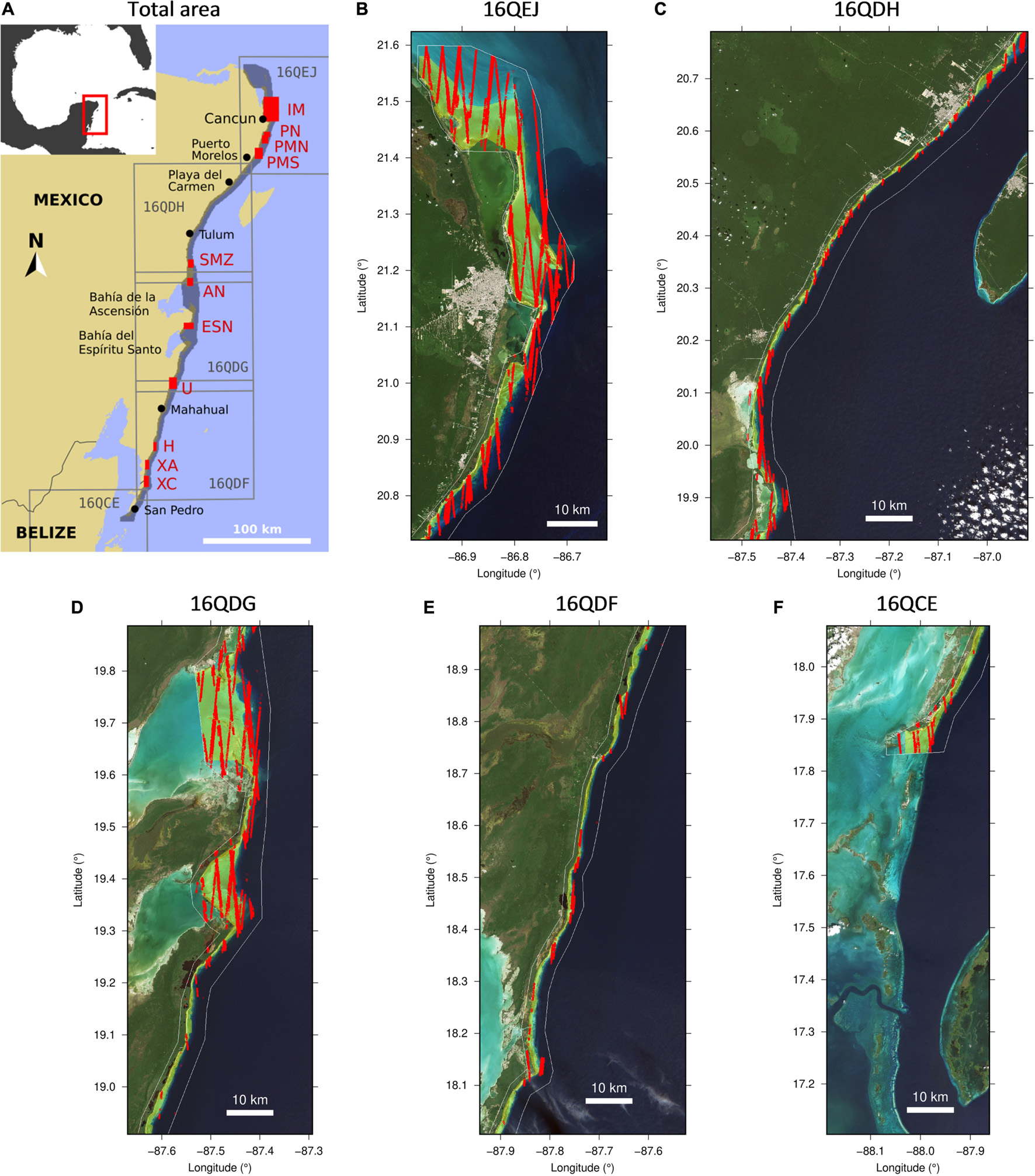
Figure 1. (A) Processed area spanning five Sentinel-2 tiles is shaded dark, sites of interest are shown in red (Table 1). (B–F) Relevant section of each tile. White line delimits the processed area. Filled yellow region is the manually delimited lagoon area. Red lines are the ICESat-2 data after screening and delimiting to the processed area, a total of 46069 points. (B–E) RGB background images are Sentinel-2 bands B04, B03, and B02 for 13 December 2017 for and (F) 24 September 2019.

Leveraging remote sensing to provide meaningful large-scale benthic mapping or change detection in shallow waters presents some challenges. The coastal environment is highly dynamic, in addition to clouds and atmospheric variations, benthic remote sensing must contend with water depth, water column constituents, floating surface materials, whitecaps and sun glint. Any particular location in any particular image could be subject to deviations that could cause errors in quantitative estimates of LAI or depth, and introduce “false positives” of change. In addition to these problems the Mexican Caribbean coastline has in recent years been subjected to “golden-tides” (Milledge and Harvey, 2016): substantial incursion of floating pelagic Sargassum which is deposited on the shoreline, then decomposes and collects in the lagoon (van Tussenbroek et al., 2017; García-Sánchez et al., 2020). While being a potential source of eutrophication, the physical presence of Sargassum, either floating or fragmented on the bottom, darkens image pixels and is largely indistinguishable from living benthos. Any remote sensing analysis of seagrass in this region must consider the potential influence of Sargassum in the interpretation.

The remote sensing analysis was implemented as an “objective” processing chain that could be consistently and repeatedly applied free from potential bias due to data or operator choices. This excluded commonly used habitat classification or machine learning approaches for seagrass mapping (Knudby and Nordlund, 2011; Lyons et al., 2013; Roelfsema et al., 2014; Traganos and Reinartz, 2018; Gapper et al., 2019) since the location and time points of training data could not be excluded as spatial or temporal bias factors (and in any case training data appropriate for the scale of the analysis was lacking). Instead, we used a radiative transfer model inversion method to simultaneously estimate LAI and depth (Hedley et al., 2016, 2017). This method was applied to the entire archive of Sentinel-2 data for the area, after only a basic cloud screening. A statistical reduction was then applied to the full set of results, taking the median LAI and depth in each pixel in each year, giving a set of results for each year from 2016 to 2020. Due to the number of images, for each year from 2017 onward each result pixel was the median of 30–40 individual estimates. This made year-to-year change detection amenable to tests of statistical significance − an apparent change between 2 years could be verified as being beyond the various influencing “noise” factors in the image-to-image analyses. The interpretation of the cause of any apparent change still requires prudence; ideally by association with known sources of natural or anthropogenic disturbance or nutrient enrichments. Constructed this way the processing chain was almost completely automated. Barring an initial “calibration” phase of choosing some basic processing parameters, the year-to-year analysis was entirely automatic. This approach made processing the entire area over 5 years tractable.

A multi-image analysis approach has previously been demonstrated as beneficial for bathymetric mapping with Landsat 8 (Ilori and Knudby, 2020). Also, Traganos et al. (2018) performed a multi-image Sentinel-2 seagrass mapping exercise using Google Earth Engine, but used median screening on the source images rather than on the output products − the disadvantage being there is no capability for statistical tests on the output products. The model inversion method used here for estimating LAI and depth has previously given good results for T. testudinum with airborne hyperspectral data (Hedley et al., 2016, 2017). A similar method has also been applied for bathymetry mapping on coral reefs with Sentinel-2 (Hedley et al., 2018). Extending the LAI analysis to multispectral imagery and exploiting the redundancy in multiple Sentinel-2 acquisitions was a natural development. Our aim was not to compare to other methodologies or evaluate this as the best approach. Rather, it was to apply a pre-existing automated method and apply a careful and critical interpretation, to see what information of practical use could be inferred from the results.

Previous field surveys have characterised the spatial and temporal variability of Thalassia testudinum leaf area, biomass, calcification rates, and productivity within the Puerto Morelos lagoon (van Tussenbroek, 1995, 1998; Enríquez and Pantoja-Reyes, 2005; Rodríguez-Martínez et al., 2010; Enríquez and Schubert, 2014; Enríquez et al., 2019) and in Bahía de la Ascensión (Medina-Gómez et al., 2016; Figure 1). Here, the interpretation of the results was informed by this background information plus a set of in situ data LAI points collected over 2016 to 2018 (Velázquez-Ochoa, Ph.D. thesis). Various “self-tests” were also performed to verify the consistency of the processing chain. In addition, bathymetry estimates were compared against ICESat-2 satellite LIDAR data, a recently available data source which is finding increasing use in bathymetry applications (Parrish et al., 2019). This data set comprised approximately 46,000 data points distributed over the entire processed area.

In summary, the overall aim of mapping the relationship between LAI and depth was split into three sub-objectives:

1) To quantify the areas of high LAI in shallow waters along the Eastern Mexican Caribbean coast; these areas comprise the primary below-ground carbon storage in Thalassia testudinum beds.

2) To understand the dynamics of a year-to-year change analysis applied to the seagrass maps, in terms of both the consistency between repeated analyses and the power for change detection.

3) To quantify the pattern of depth and LAI across the region and map deviations from the relationship previously determined by local-scale field study.

Materials and Methods

Site and Field Data

The Mexican Caribbean coast has been affected by 50 years of tourism development, but in a spatially uneven pattern (Torres and Momsen, 2005). In the early 1970s the Northern coast island of Cancún initiated its transformation to a mass tourism destination, becoming the first Tourist Integral Centre (TIC) of Mexico (Vargas-Martínez et al., 2013). In the 1980s the tourism development migrated south with the construction of a significant number of “megaresorts” from Cancún to Tulum, giving origin to the “Riviera Maya” (Torres and Momsen, 2005). In parallel to this development, the Sian Ka’an Biosphere Reserve was established in 1986 in the municipality of Tulum and became a UNESCO World Heritage nature reserve in 1987, covering an area of 5,280 km² around two large bays: “Bahía de la Ascensión” and “Bahía del Espíritu Santo” (Figure 1). South of this protected area the “Costa Maya” continues to be relatively undeveloped with small coastal populations. Only the small town of Mahahual (<1,000 population) has some relevant tourism activities, with a cruise-ship port operating since 2001 (Meyer-Arendt, 2009). Different parts of the coastline have been affected by hurricanes: three category-5 hurricanes in the last 20 years (Wilma in 2005, Dean in 2007, and Delta in 2020), plus a significant number of smaller ones. In addition, weather events, called “Nortes” (north), with cold winds from the Gulf of Mexico of over 60 km per hour, are prevalent during the cold season. Local fisheries are also active along the coast. The reef community of this area has been extensively studied (e.g., González-Barrios and Álvarez-Filip, 2018; Guimarais et al., 2021).

The area of interest for the remote sensing analysis was the mainland east-facing coast of Yucatán from the northern-most point above Cancún, to the channel south of San Pedro in Belize, approximately 460 km of coastline in total. The coastal geomorphology is typified by a lagoonal area between the reef crest and sandy beach, which varies in width from just a few hundred metres up to 3 km at Punta Nizuc, at the northern end of the 22 km long lagoon that runs from Puerto Morelos north to just south of Cancún (Figures 1A,B). This lagoonal area has been well studied and is the primary source of information about Thalassia testudinum population biology and ecology in the region. In particular, this is the location of the Coral Reef Research Unit of the Universidad Nacional Autónoma de Mexico (UNAM), the Mesoamerican Centre of Excellence within the World Bank / GEF Coral Reef Research Project (GEF, 2010). Southward along the Yucatán coast numerous similar but smaller lagoons occur, which have similar bio-geographical features. Commonly, the lagoonal areas have a depth profile that increases gradually from the shore to a maximum of 5–6 m, but punctuated by channels that can be deeper. Where channels occur, and in some other places, the reef crest is absent and the lagoon is less well defined, delimited by a rapid bathymetric drop-off into waters of ∼40 m depth or more. Water enters lagoonal areas by wave action over the reef crest, and exits via potentially strong flows through the channels (Coronado et al., 2007).

Thalassia testudinum is the dominant climax seagrass species in the lagoonal areas, smaller seagrasses such as Syringodium filiforme and Halodule wrightii are also present together with various benthic macroalgae (predominantly calcifying species). As part of ongoing fieldwork 26 data points of canopy LAI were collected over years 2016, 2017, 2018, primarily in the Puerto Morelos lagoon area, but with some additional more southern points. These data were collected by sampling from 0.25 × 0.25 m quadrats with 5 to 8 replicates per station. Note that LAI refers to single sided leaf area index, being the ratio the leaf area to area of substrate, and was estimated by multiplying the shoot density per quadrat by the overall shoot size average across the replicates.

Sentinel-2 Data and Processed Area

The Mexican Caribbean mainland coast extends over five Sentinel-2 tiles (Figure 1). All available Sentinel-2 tiles from the start of 2016 to the end of 2020 were initially downloaded. Approximately 30% were rejected by visual inspection where cloud cover was so extensive that processing the tile would have offered little useful information. This left between 134 and 180 images in each tile. Sentinel 2A (S2A) was launched in June 2015 but only data starting in January 2016 was used. Sentinel 2B (S2B) was launched in 2017 and data is available from July 2017. Therefore, data from mid-2017 included both S2A and S2B in roughly equal proportions and 2017 has higher data representation in the second part of the year than the first. The change detection analysis was applied to data grouped in years to avoid any seasonal biases, but with respect to 2017 this is slightly compromised by more images later in the year. Ultimately, 2017 was represented by 13 to 24 images in each tile while 2018, 2019, and 2020 had 31 to 51 images in each tile. Supplementary Table 1 lists the number of images processed in each tile and year.

Full tiles were used in the pre-processing steps up to and including atmospheric correction, but depth and LAI processing was restricted to the coastal area from a thin strip of land to deep water (Figure 1). The area for LAI interpretation was further restricted since the LAI estimation is relevant only over lagoonal areas, not over corals or deep water. An area of interest (AOI), henceforth referred to as the “lagoon area,” was manually defined from land to the inside edge of the reef crest or flat, or to the slope where the crest was absent. The total lagoon area was 904 km², while the full processed area was ∼3,500 km². In addition, to organise the results, eleven sites of interest distributed along the coastline were defined as listed in Table 1. Each site was a section of the lagoon area for a stretch of coastline and ranged in area from 4.5 to 15.7 km², plus one large site north of Cancún of 125.4 km² (see also Supplementary Material). The sites cover the full north to south range of the analyses and include two sites in the bays in the Sian Ka’an Biosphere Reserve which are influenced by freshwater outflow (AN, ESN, Table 1). Area-averages of the various analyses were produced from these sites to investigate large-scale trends. The processed area, lagoon area, sites of interest, and the location of the ICESat-2 data (discussed in the next section) are shown in Figure 1.

TABLE 1

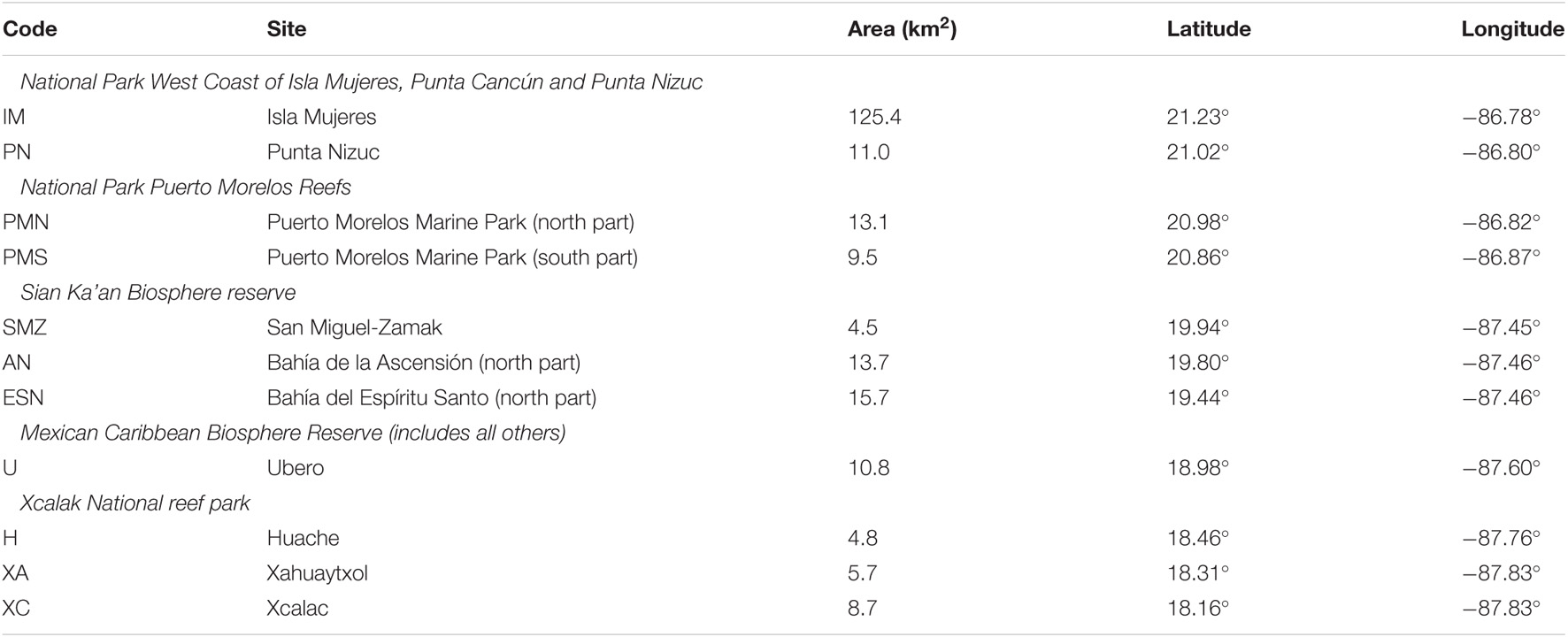
Table 1. The eleven sites of interest referred to in the results, listed north to south and indicating the marine parks or reserves they are contained within.

Sentinel-2 images consist of 13 bands covering a total wavelength range from 433 to 2,286 nm, with various bands collected at 10, 20, and 60 m pixel resolutions (SUHET, 2015). Since water is practically opaque to wavelengths longer than 700 nm the analysis only made use of Sentinel-2 MSI bands B01 to B05 (433–453 nm, 460–525 nm, 543–578 nm, 650–680 nm, 698–712 nm) plus B08 (783–888 nm) for land and cloud screening. All processing was at the native 10 m pixel resolution of bands B02 to B04 with bands B01 and B05 upscaled from 60 and 20 m without interpolation.

ICESat-2 Data

The ICESat-2 satellite launched in 2018 and carries the ATLAS (Advanced Topographic Laser Altimeter) instrument, which provides altimetry data from six laser transects along-swath (Figure 1). The lasers are arranged in pairs of weak and strong beams providing three basic transects separated by approximately 3 km, and 90 m within pairs. The beam footprint is approximately 17 m. The ALTAS sensor is not designed to provide bathymetry data, but under favourable conditions photon returns from the water surface and seabed can be detected in the data for depths of up to 40 m. The data is extremely noisy, however, no specific bathymetry product is provided so the data requires manual corrections and screening. The primary correction required is to compensate for the reduced speed of light in water and a change in the refraction angle if incidence angle is non-nadir, these give rise to a correction for both vertical and horizontal error. The full calculation is given in Parrish et al. (2019). However, here, no data had an incidence angle greater than 2.3°, giving a maximum horizontal error of 0.5 at 30 m depth, negligible for 10 m Sentinel-2 pixels and 17 m laser footprint. The only correction applied was therefore the depth estimate correction, z’ = z/1.34 where 1.34 is assumed as the refractive index of water.

All of the ICESat-2 ATLAS photon return data which intersected with the processed area were downloaded (Neumann et al., 2021). This was a total of 456 files (each file represents one laser) from 16 October 2018 to 7 July 2020, of which ultimately 239 files had useful data. The photon return data was clipped to the area of interest, and converted into images with the x-axis along transect, and y-axis vertical (i.e., depth), and each pixel value being the number of photon returns at a resolution of 10 m (horizontal) × 0.1 m (vertical). A basic pixel density algorithm was applied to filter out isolated noise points and leave denser areas of photon returns. Finally the image was manually cleaned using a “paint” style software tool, to remove stray points that were not either water surface or sea bed, by visual inspection. The cleaned image was reprocessed to extract the lat-long and depth points. Tide correction was applied using OTPS2 (Egbert and Erofeeva, 2002) but the tidal variation in the region was only ± 0.17 m over all the data, less than the noise level in the points. The final size of the dataset was 46,069 points in the processed area (Figure 1). For comparing to estimated depths only the 0–15 m range was used and the points were evenly depth stratified by randomly removing points so that the intervals 0–5 m, 5–10 m, and 10–15 m each had the same number of points. This is important to avoid bias in statistical metrics due to the depth distribution of data points and is advised for meaningful comparison between studies.

The ICESat-2 data was used only for validation of output depths. This included visual inspection of the scatter plots and initial iteration on the best choice of some basic processing parameters, such as which Sentinel-2 bands to use and the range of sand reflectance to include (described below). This could therefore be described as a “calibration” exercise, to the same extent that any re-analysis of imagery to improve results turns “validation” data into “calibration” data.

Land and Cloud Masking Data

To facilitate processing a large number of images, land and cloud masking was largely automated. The automation relies on various threshold values that were deduced just by visual interpretation as part of the initial setup of the analysis. At another site these parameters may need to be adjusted.

A land mask was created for each year by applying a threshold of 1,500 DN (i.e., reflectance of 0.15) in band B08 (NIR, 784–900 nm) to each Sentinel-2 tile in that year, pixels masked in more than 75% of the images in a year were flagged as land. Then a “flood fill” operation was applied from a user-identified deep water point in order to clean up the mask, removing any stray unmasked points or inland water bodies in the land area. After an initial iteration of this automated process, a few areas such as rivers were identified which would preferably be masked, and a manual mask modifier was created (by “painting” an image) so that these areas would be blocked off when the flood fill was applied. A land mask was created independently for each year, rather than one overall mask, as this strategy means the analysis can be extended in future years without requiring any reprocessing.

For each individual tile a cloud mask was created by applying a threshold of 900 DN (i.e., reflectance of 0.09) to band B08. This method did not mask thin cloud and neither did it mask cloud shadows; we relied on the outlier rejection of the final ensemble analysis for this.

Atmospheric Correction

Model inversion methods operate in radiometric units, and so require atmospheric correction. The method used here was the deep water calibration method (DWC, described in Hamylton et al., 2015; Hedley et al., 2018; Casal et al., 2020). The essence of the method is that two parameters, aerosol optical thickness and wind speed (a proxy for surface roughness), are estimated on the premise that optically deep water should be estimated as deep when processed in the inversion model (described in the next section). Effectively, an inversion is applied to a selection of deep water pixels to estimate the atmospheric parameters and water column parameters at the same time (Kutser et al., 2002, 2006), but constrained so that only depths greater than 20 m are allowed and the atmospheric parameters are the same everywhere. Note that this does not mean 20 m is necessarily “optically deep,” but that a depth estimate of 20 m or more would be considered a reasonable result in a deep water area. The correction was applied to whole tiles, and so assumes the estimated atmospheric parameters are constant across the tile, which is in general not true but is a practical compromise.

Previous applications of this method required the operator to manually select a set of deep water areas, but here this process was automated. First, the cloud mask for an image was grown outward for 100 iterations, where a pixel became included in the mask if one of its neighbours is in the mask. This put a 100 pixel (1 km) buffer around any initially masked pixels and helped to exclude thin peripheral cloud. Potential deep water pixels in a Sentinel-2 tile were identified by establishing a spatially smoothed “blue-green map” for each year, as the median of the squared sum of bands B02 and B03 in non-masked pixels across all images in the year, filtered by a 400 × 400 pixel mean filter. Tiles were subdivided into a regular 6 × 6 grid of regions and for each individual image ten 5 × 5 pixel deep water AOIs were created at random across different grid locations in places which were non-masked and where the AOI centre pixel was below the 50% percentile (i.e., median) value of the blue-green map. Note that this threshold, deduced heuristically, is likely reliant on the tile area being more than 50% deep water (Figure 1A). Simply put, the method places deep water AOIs in places that are dark in bands B02 and B03 in comparison to what is typical across the tile area (and not cloud or land masked). The atmospheric correction was then calibrated using the mean pixel reflectance in each of these 10 AOIs. Only bands B01 to B05 were corrected (430–713 nm).

Unlike previous applications of a similar processing chain (Hedley et al., 2018; Casal et al., 2020) surface glint correction was not applied (Hedley et al., 2005). This glint correction is based on a near-infra red (NIR) band and can over-correct over shallow dense vegetation where water-leaving NIR may not be zero (Kutser et al., 2009). Instead, we relied on the multi-image analysis to reject glint contaminated results. This was considered sensible as our primary interest was vegetation in the lagoonal areas, and in the lagoon the water surface is typically flatter and less susceptible to glint anyway.

Depth and Leaf Area Index Forward Model

Processing of the atmospherically corrected Sentinel-2 data was conducted by a model inversion or “physics-based” methodology (Figure 2; Hedley et al., 2016, 2017). This involves spectral matching the outputs of a radiative transfer model to the image data. This “forward” model outputs the spectral water leaving reflectance, R_rs(λ), for a given set of feature parameters, including water depth, water column constituents and canopy LAI (Figure 2J). The spectral matching “inverts” this model to give estimates of depth and LAI at every pixel.

FIGURE 2

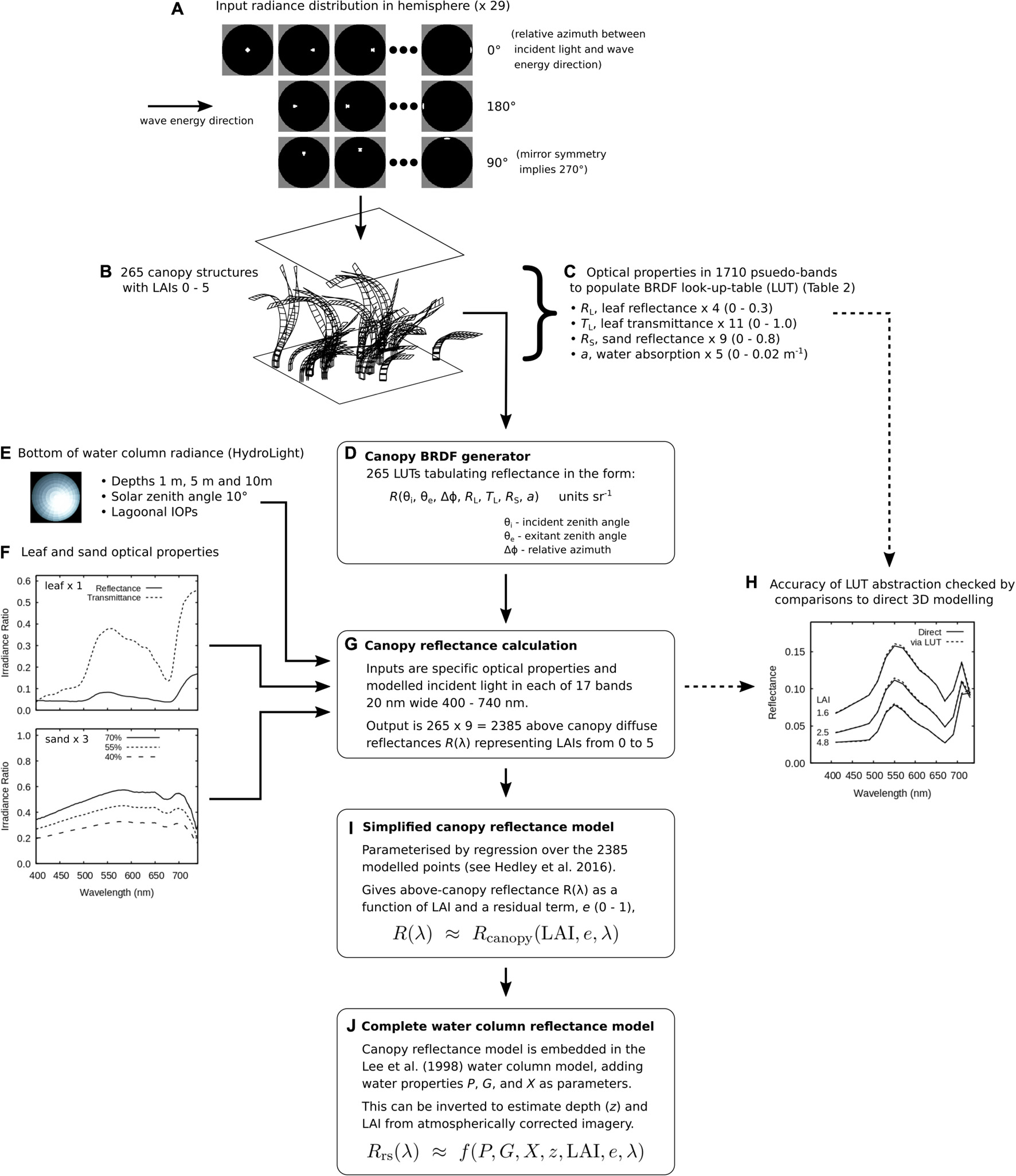
Figure 2. Construction of the forward model. (A–C) A 3-dimensional canopy model is used to populate (D) a look-up-table, which combined with (E,F) material optical properties and incident radiance (G,H) generates above-canopy spectral reflectances. (I) A set of these reflectances parameterises a simplified bottom reflectance model which is (J) embedded in the Lee et al. (1998) semi-empirical water column model.

The model used here is described in detail in Hedley et al. (2016, 2017). The basic form is the Lee et al. (1998, 1999) semi-empirical model for shallow water reflectance (see Hedley et al., 2009 for a concise list of the equations) modified such that the bottom spectral reflectance component is given by two parameters, LAI (ranging 0 to 5), and a residual term, e, (0 ≤ e ≤ 1) that encompasses variation due to canopy structure, position and incident light field (Figure 2I). This model in turn is parameterised from a 3-dimensional canopy model (Figures 2A–C; Hedley, 2008; Hedley and Enríquez, 2010). In previous work the spectral reflectance and transmittance of leaves, R_L(λ) and R_T(λ), and the reflectance of the substrate, R_S(λ), was required to be specified prior to the 3D modelling, requiring extensive re-computation to generate functions for different leaf or sand optical properties. Here, a method was developed to abstract the 3D canopy structure from the material optical properties, allowing the leaf and sand optical properties to be specified after the 3D modelling (Figure 2). This was achieved by performing the 3D modelling with “pseudo” reflectances, transmittances, and within-canopy water absorption in order to populate a look-up-table. Linear interpolation could then generate a BRDF function, or above-canopy spectral reflectance, for any combination of specific material optical properties (Figure 2D). Comparison to directly modelled reflectances showed that the deviations introduced by this abstraction were negligible compared to the variation across canopy structures (Figure 2H and Hedley et al., 2016).

This abstraction of the canopy model is a technical detail that can ignored, apart from that it facilitated an initial calibration exercise where the optimal sand reflectance was determined. The T. testudinum leaf reflectance and transmittance (Figure 2F) were fixed as used in Hedley et al. (2016) but initial results using a sand reflectance spectrum previously used in bathymetry work (Hedley et al., 2018, and Figure 2 in 2012) were poor by visual inspection and when compared against the ICESat-2 depth data. It was determined that the sand reflectance was too bright when used in the relatively simple LAI bottom reflectance model: in comparison, the previous bathymetry work used a multi-endmember linear mixing model (spectra in Hedley et al., 2012). Iteration on a few options indicated that a set of three sand reflectances being 40–70% scaled versions of the original reflectance (Figure 2F) produced better results. In addition, excluding the far red band B05 (697–713 nm) was advantageous (this may be related to the lack of surface glint correction). This initial setup was the only modification made to the model compared to previous work (Hedley et al., 2016, 2017, 2018). In particular, the ranges of the water column parameters P, G, X (Figure 2J) were the same as used in Hedley et al. (2018). Anecdotally, these ranges have been used in a large body of unpublished bathymetry work and for tropical coastal environments changing them has never been found to improve the accuracy (Hedley, unpublished data). The permitted depth range (z) was 0 to 30 m. The maximum LAI the model inversion can report is 5, this limit was based on previous work which indicated the reflectance of canopies does not detectably change for higher LAIs (Hedley et al., 2016).

Model Inversion and Post-processing

The forward model is computed hyperspectrally in 2 nm intervals and convolved to the Sentinel-2 relative spectral response functions at the point of spectral matching. Inversion of the model was performed by the adaptive look-up table (ALUT) method (Hedley et al., 2009), this gave estimates of depth and LAI for each unmasked pixel of each image from 2016 to 2020. From these, for each year and tile, LAI and depth layers were produced by taking the median value in the non-masked pixels across all the image outputs for that year, in the results these are referred to as the “year-median” depth or LAI. For each year the five median tile outputs were mosaicked together, with the data from the northern-most tile taken in areas of overlap.

Since the LAI estimation cannot distinguish between Thalassia testudinum and other macrophytes such as smaller seagrasses and macroalgae, the estimated LAI may comprise mixed canopies. However, T. testudinum is the dominant species in these seagrass meadows, field data shows that other species typically comprise less than 0.5 LAI units of the total community LAI, and in particular LAIs above 3 are almost entirely Thalassia testudinum (Velázquez-Ochoa, Ph.D. thesis, Supplementary Figure 1).

For comparison to point data, a 3 × 3 pixel mean filter was applied to the year-median depth layers, but the year-median LAI layers were not filtered. Previous work has shown that taking a spatial mean improves comparison to point depth data (Hedley et al., 2018). In fact, visual inspection of successive images indicated that their spatial alignment is at best ± 1 pixel (10 m). Therefore, although processed at 10 m resolution the outputs cannot be considered to be meaningful at that resolution. For change detection, 3 × 3 pixel mean filters were applied to both depth and LAI, and for mapping LAI-depth regimes, 5 × 5 pixel mean filters were applied. In these analyses broader patterns were of interest, filtering makes the plots cleaner and removes some “salt and pepper” pixel noise.

Leaf Area Index Change Detection

The five year-median LAI maps from 2016 to 2020 were compared pair-wise for changes in successive years, and for a longer-term comparison 2017 was compared to 2020 (2017 was preferred over 2016 due to having more images). Since the metric of interest was the median LAI over a year, a median test (sometimes referred to as Mood’s median test, Salkind, 2007) was conducted for each pixel in the map, comparing the values for that pixel in the two samples from the images of the years to be compared. The test is essentially a chi-squared performed on the contingency table from the null hypothesis that the populations have the same median. As the median test was performed on many millions of pixels it was anticipated that “false positive” type 1 errors might be abundant. This was prepared for in several ways:

1) The level of significance for rejecting the null hypothesis of no change was set at 1% (p < 0.01) rather than 5%.

2) Only significant differences above a certain magnitude change in median LAI were accepted, various analyses were performed with this threshold being between 0.5 and 0.1.

3) The whole processed area was subjected to the change analysis, not just the LAI (lagoon) area. The rationale was that changes identified over deep water, for example, could be indicative of systematic image or processing errors (e.g., what if an aerosol event occurred in one year?). This would be useful counter-check for the interpretation.

4) A self-test was performed by applying change detection over areas where different Sentinel-2 tiles overlapped within the same year. In this situation no change should be detected and so this would indicate if apparent changes were at the level of variation caused by noise or processing artefacts (However, the stringency of this test is limited by the fact that all source tiles were from the same Sentinel-2 swath and not independent acquisitions).

5) Randomised tests were performed where at each pixel the data for the 2 years was randomly split into two samples, which the median test was then performed on. Any detected changes would certainly be false positives and so indicate the limit of the power of the test.

6) Finally, statistical type 1 errors would be random and independent of spatial context, and so the extent of the problem should be apparent by visual interpretation.

The basic sample size for the median tests was the number of images in each group for each tile (Supplementary Table 1). However, at each individual pixel the sample size varied, since in some images the pixel was cloud masked. Nevertheless, in the vast majority of cases from 2018 onward n for each year was in the range 30–45 at each pixel.

Leaf Area Index-Depth Regime

Fieldwork on Thalassia testudinum canopies in the Puerto Morelos reef lagoon in 2004 established a negative exponential reduction with depth for the LAI that occurs at climax seagrass colonization (Enríquez et al., 2019). Typically, LAIs of 4 or more are only found in the shallowest coastal fringe (<2 m depth) and as the lagoon deepens LAI decreases to less than 2 by depths of 4 m. However, this climax state is not always observed. Water movement, disturbances by “Nortes” winds, or sediment deposition can prevent seagrass establishment and may determine patterns of seagrass colonization (Cunha et al., 2005; Cabaço et al., 2008). In tropical areas, strong climatic events such as storms and hurricanes may cause significant and species-specific seagrass losses (Rodríguez et al., 1994; Hernández-Delgado et al., 2020), T. testudinum has a slower capacity of recovery after disturbance than the pioneer species in the community. Moreover, capacity for recovery also depends on nutrient availability, which often limits seagrass growth in oligotrophic reef environments (Fourqurean et al., 1992). Thus, the balance between seagrass recovery and local disturbances may explain the areas of low seagrass colonisation at depths where in other contexts seagrasses are found, and the patchy nature of seagrass distribution. Conversely, increases in nutrient availability can cause positive deviations from the oligotrophic climax state, as habitat fertilisation favours increases in shoot growth, leaf area per shoot and above-ground biomass (Short, 1987; Frankovich and Fourqurean, 1997).

As background for the remote sensing analysis, building on the LAI-depth model published in Enríquez et al. (2019), a database of Thalassia testudinum LAI and depth was developed from a literature survey plus additional field determinations of LAI in this area (n = 244, Velázquez-Ochoa and Enríquez, unpublished data). While the majority of the new data was consistent with the model of Enríquez et al. (2019) some data indicated potential higher upper bounds for LAI. The information is summarised in Figure 3A, which includes two least-squares fit lines to the data from Enríquez et al. (2019) and the upper bounds of the new extended data, respectively:

$$\mathrm{EOCH2019}\mathit{\hspace{1em}\hspace{1em}\hspace{0.5em}\hspace{0.25em}}{\text{LAI}}_{\text{MAX}}=0.226+6.553\times \text{exp}\left(-0.849\times z\right)(1)$$

$$\mathrm{extended}\mathrm{model}\mathit{\hspace{1em}\hspace{1em}\hspace{1em}\hspace{1em}\hspace{1em}\hspace{0.25em}}{\text{LAI}}_{\text{MAX}}=6.036\times z^{-0.634}(2)$$

FIGURE 3

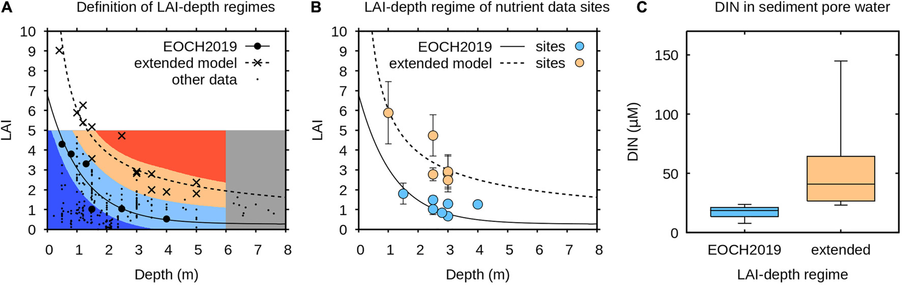
Figure 3. (A) Data on maximum Thalassia testudinum LAI as a function of depth from Enríquez et al. (2019) (EOCH2019) and the extended model (Velázquez-Ochoa and Enríquez, unpublished data). Lines are least-squares fit to the data of an exponential and power model, respectively (Eqs. 1 and 2). Small dots show all depth and LAI determinations (n = 244). Background colour is as used in results figures. (B) LAI and depth of sites for nutrient determination. (C) Dissolved inorganic nitrogen (DIN) in the sediment pore water at the sites shown in (B), box plots show median, quartiles and range, medians are significantly different with p < 0.01 (Mann-Whitney U test).

Our interest in the satellite image analysis was to understand the pattern of LAI-depth regime across the entire Eastern Mexican Caribbean coast in relation to these two models. To achieve this, the 5 × 5 pixel filtered year-median LAI and depth layers were plotted according to colour scheme shown in Figure 3, which was designed to indicate where the LAI-depth regime was closest to EOCH2019 (Eq. 1) or the extended model (Eq. 2), and also where it lay outside of either domain. This analysis was restricted to depths less than 6 m and LAIs of 0–5.

Figure 3 also shows measurements of sediment pore dissolved organic nitrogen (DIN) collected at 12 sites in 2016–2018 from various locations along the coast. The sediment DIN is significantly higher at the sites corresponding to the extended model (p < 0.01, Mann Whitney U test). This suggests a direct relationship between nutrients, meadow productivity and canopy LAI, and also confirms that the EOCH2019 model characterised in 2004 corresponds to an environment with lower nutrients available for seagrass growth.

Results and Discussion

Overview

Qualitatively, the output maps of LAI and depth agree with visual interpretation of the images (Figure 4). In particular, LAI was zero over bare sand and took a maximum value of around 4 over dense shallow canopies close to the shore (Figure 4C). This is consistent with the previously reported pattern of LAI in this area (Enríquez et al., 2019). Since previous work indicates that LAIs above 4 cannot be distinguished by remote sensing (Hedley et al., 2016) the LAI maps should be interpreted such that values of around 4 could be in reality 4 or greater. The depth map is also qualitatively reasonable, being shallow close to shore, progressively deeper in the lagoon and deeper at outflow channels (Figure 4B). The shallow reef crest can also clearly be seen.

FIGURE 4

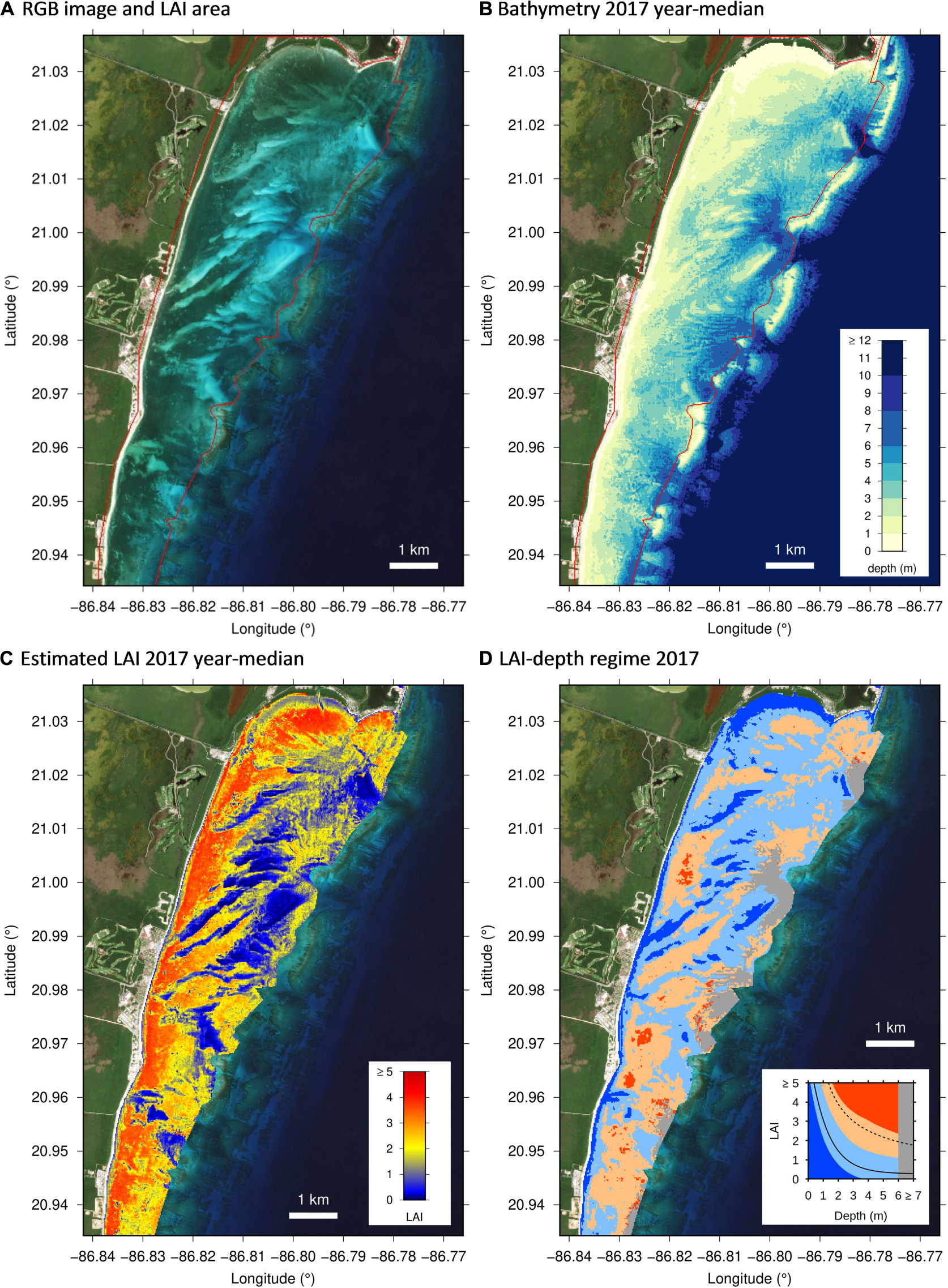
Figure 4. Example results from the northern part of the Puerto Morelos lagoon. (A) RGB image from 13 December 2017, (B) 2017 year-median depth, (C) 2017 year-median estimated LAI, (D) LAI-depth regime for 2017 based on (B,C). Red line in (A,B) is the limit of the LAI area of interest.

Depth

Estimated depths compared to the ICESat-2 data show good agreement with a systematic bias less than half a metre up to 15 m depth in any of the 5 years (Figure 5), at the full scale of the processed area. The ICESat-2 data spans 2018 to 2020 and was treated as a single data set, but nevertheless the comparisons to bathymetry results from each individual year from 2016 to 2020 were similar (Figures 5A–E). This indicates that, at the temporal and spatial scales involved, grouping the ICESat-2 data over 2018 to 2020 is inconsequential to the interpretation. The statistics reported in Figure 5 are from depth stratified data over 0–15 m and give a mean absolute error of approximately one metre. Since the spread increases as a function depth (Figure 5) for our interest in depths < 6 m the error will be less. Part of the apparent spread arises from the extraction of bathymetry from the ICESat-2 data; these estimates cannot be more accurate than ± 0.1 m and probably are only reliably accurate to ± 0.3 m, at best.

FIGURE 5

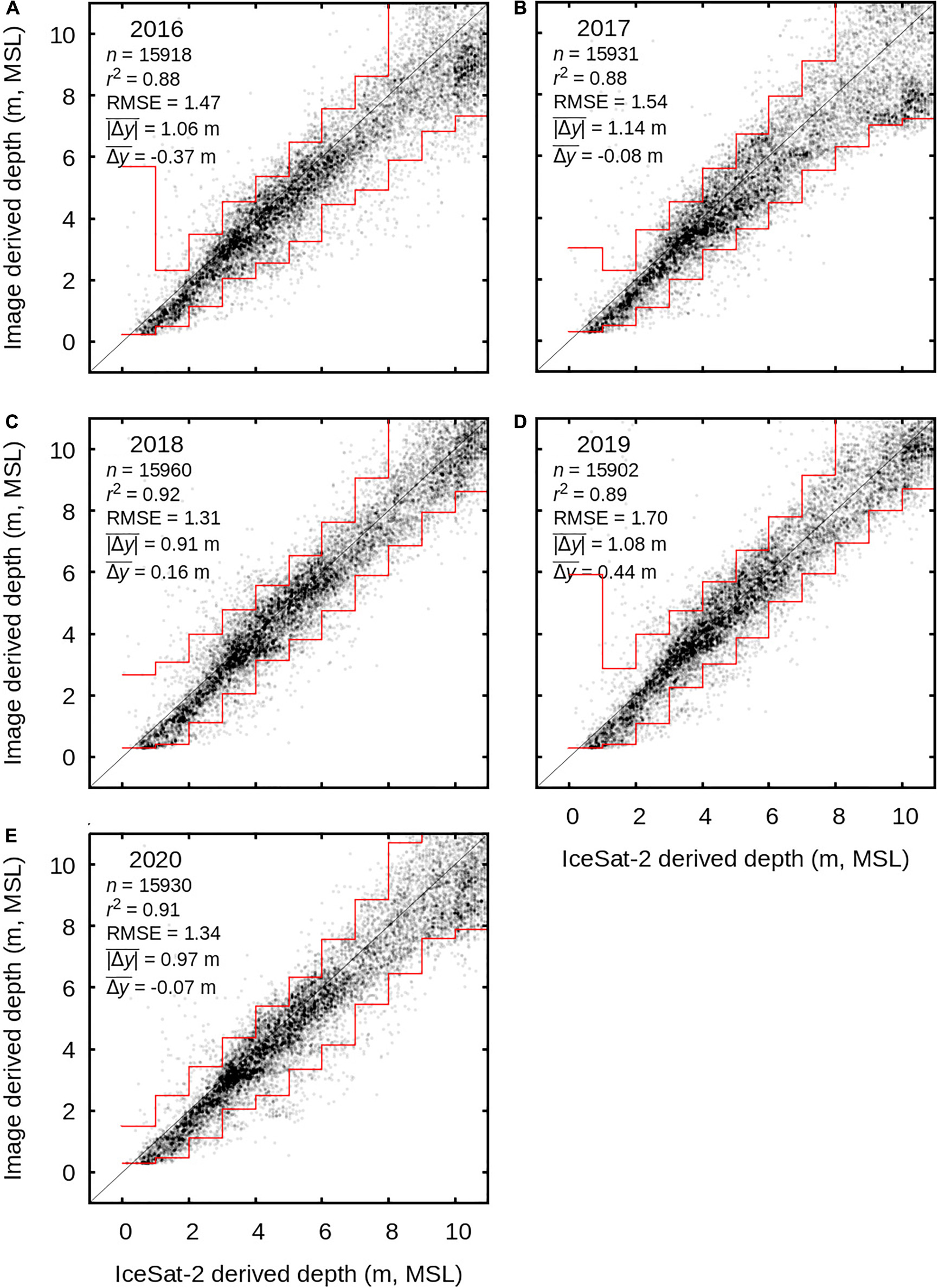
Figure 5. ICESat-2 depth data compared to image derived year-median depths over the entire processed area. (A–E) show years 2016 to 2020. The ICESat-2 data spans 2018–2020 but was treated as a single data set and has been randomly subset to ensure even depth stratification from 0 to 15 m in 5 m bins (i.e., there are n/3 points in 0–5 m, 5–10 m, and 10–15 m). Statistics are calculated over 0–15 m. In each 1 m step 95% of the points lie between the red lines.

Leaf Area Index

Regarding the LAI estimates, the majority of the 26 field data LAI points cluster around the 1:1 line with a few outliers − in particular two under-estimated values for LAIs greater than 4 (Figure 6). The LAI field data was collected in the context of work on canopy ecology (not remote sensing) so lacks data points with LAI of zero, however, visual interpretation of the results (Figure 4) indicates good ability to estimate LAI of zero over bare substrate. It is therefore justifiable to calculate r-squared from a zero-constrained regression, which gives r² = 0.67 for all points and r² = 0.83 if the two high LAI outliers are omitted. In fact, the issue with the high LAI outliers is largely geo-location (Figure 7). In the imagery the points numbered 1 and 2 lie on relatively bare sand close to narrow dense LAI areas, so most likely the positioning in the image is in error. Omitting those two points gives a mean absolute error in LAI estimates of 0.59, and a systematic error of 0.04. The regression slope is 0.89 with 95% confidence intervals of ± 0.17, hence not significantly different from 1. While r–squared is not an ideal metric for assessing the LAI estimation it does allow comparison to previously published hyperspectral applications of the method, which reported values of 0.64 and 0.86 vs. 0.83 here (Hedley et al., 2016, 2017). Overall, in terms of a large-scale synoptic view, especially of the densest canopies, using multispectral data did not seem to impair the accuracy and the basic pattern of the LAI map was of sufficient accuracy for the aims of the study (see also the Figures in the Supplementary Material).

FIGURE 6

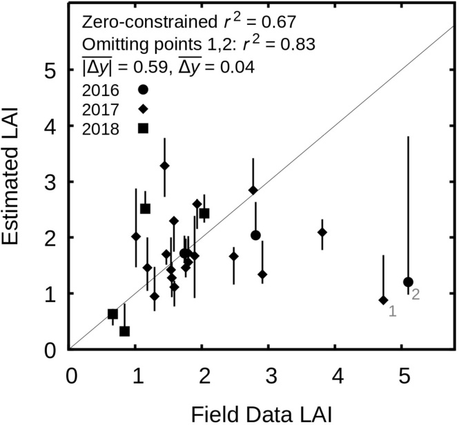
Figure 6. Scatterplot of LAI field data vs. image derived year-median LAI for the year each data point was collected (shown in the key, n = 26). Grey line is 1:1, error bars are the minimum and maximum LAI value found in the 5 × 5 pixel window centred on the pixel containing the field data point. Points labelled 1 and 2 are mentioned in the text and shown in detail in Figure 7.

FIGURE 7

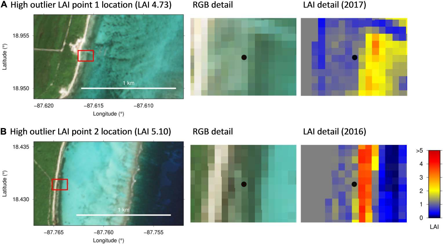
Figure 7. Detail of the two outlier points with LAI greater than 4, as shown in Figure 6: (A) point 1, (B) point 2. Left images show the general location of each data point in the imagery, the red rectangle represents the area shown in detail in the images on the right. The dot in the centre of the detailed images is the location of the point, pixels are 10 m × 10 m. The RGB images are Sentinel-2 bands B04, B03, and B02 and are from 13 December 2017. LAI images are the year-median results for the year each data point was collected in.

Influence of Bottom Reflectance on Depth Estimation

While Figure 5 suggests that at large scales bathymetry is unbiased, it does not show the detail of what happens over light and dark bottoms, where some confusion between bathymetry and LAI might be expected. Figure 8 shows a single ICESat-2 transect over a gradient in depth and a range of bottom reflectance from bright sand to dense canopy. Comparing the depth transect with the ICESat-2 data (Figure 8B) indicates that small errors in the bathymetry can occur as a function of bottom reflectance, but overall, the depth transect shows excellent consistency with the ICESat-2 data. Four locations where differences between ICESat-2 depth estimates and the 2020 year-median image estimates occur are marked in Figure 8B. Regions 1, 2, and 3 indicate the potential for image depth estimates to be influenced by bottom reflectance in shallow areas, with a full range error of around ± 0.5 m, i.e., 0.5 m too deep over dense LAI and 0.5 m too shallow over bright bottoms in depths less than 3 m. Region 4 of Figure 8B shows the opposite, where ICESat-2 depths of around 7 m are estimated at around 6 m from the image analysis, but over relatively dark bottom reflectances. This level of potential error must be borne in mind for the interpretation, but for the purpose of mapping seagrasses a depth estimate error of 0.5 m is not especially large.

FIGURE 8

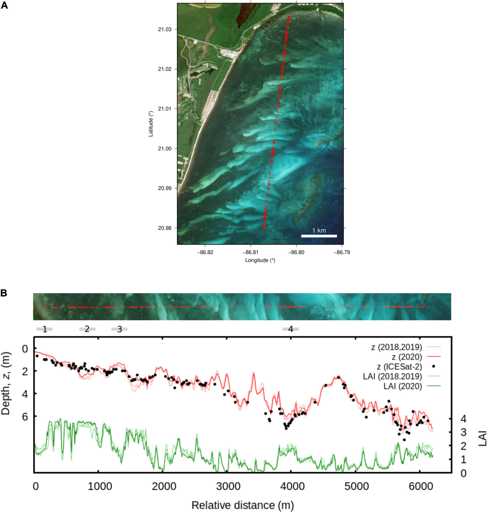
Figure 8. (A) Transect of ICESat-2 data points from 2 February 2020, n = 140. (B) Plot along transect starting at the top of (A) showing depth from image analysis (z, red) and ICESat-2 data (dots), and estimated LAI (green). Dark red and dark green lines are estimates from the 2020 image median, 2018 and 2019 image medians are also shown as lighter coloured lines. Sections indicated by “1” to “4” are referred to in the text.

From Figure 8 it can also be seen that the estimates of depth and LAI are quite consistent between the year-median results for 2018, 2019, and 2020 but some variation does occur. For example, in the year-median results for 2018 and 2019 there is an apparent overestimation of depth similar to the feature marked “2” but at the position ∼1,600 m, which is not the case in 2020 year-median. Since, at this level of detail, there is no data to conclusively differentiate real changes from sensitivities in the results, this level of variation is most safely interpreted as an upper bound on noise level in the results.

Change Detection

Given the large scale of the analysis, and the reliance on taking year-medians to remove outliers caused by a variety of processes, it was anticipated that the change detection analysis might identify a large number of “meaningless” changes (i.e., type 1 errors). In practice, for successive years (Figure 9), and between 2017 and 2020 (Figure 9D), changes in year-median estimated LAI identified at the 1% level were spatially plausible and limited in extent. The results show patches of increase and decrease were often aligned with canopy edges indicating spatial extension or retraction. In particular there are relatively few “false positives” over deep water, although the analysis does pick up changes on the reef crest, which are outside the lagoon area so do not represent seagrasses, these may relate to corals or algae. While out of scope for this study, this may be information of relevance to reef monitoring.

FIGURE 9

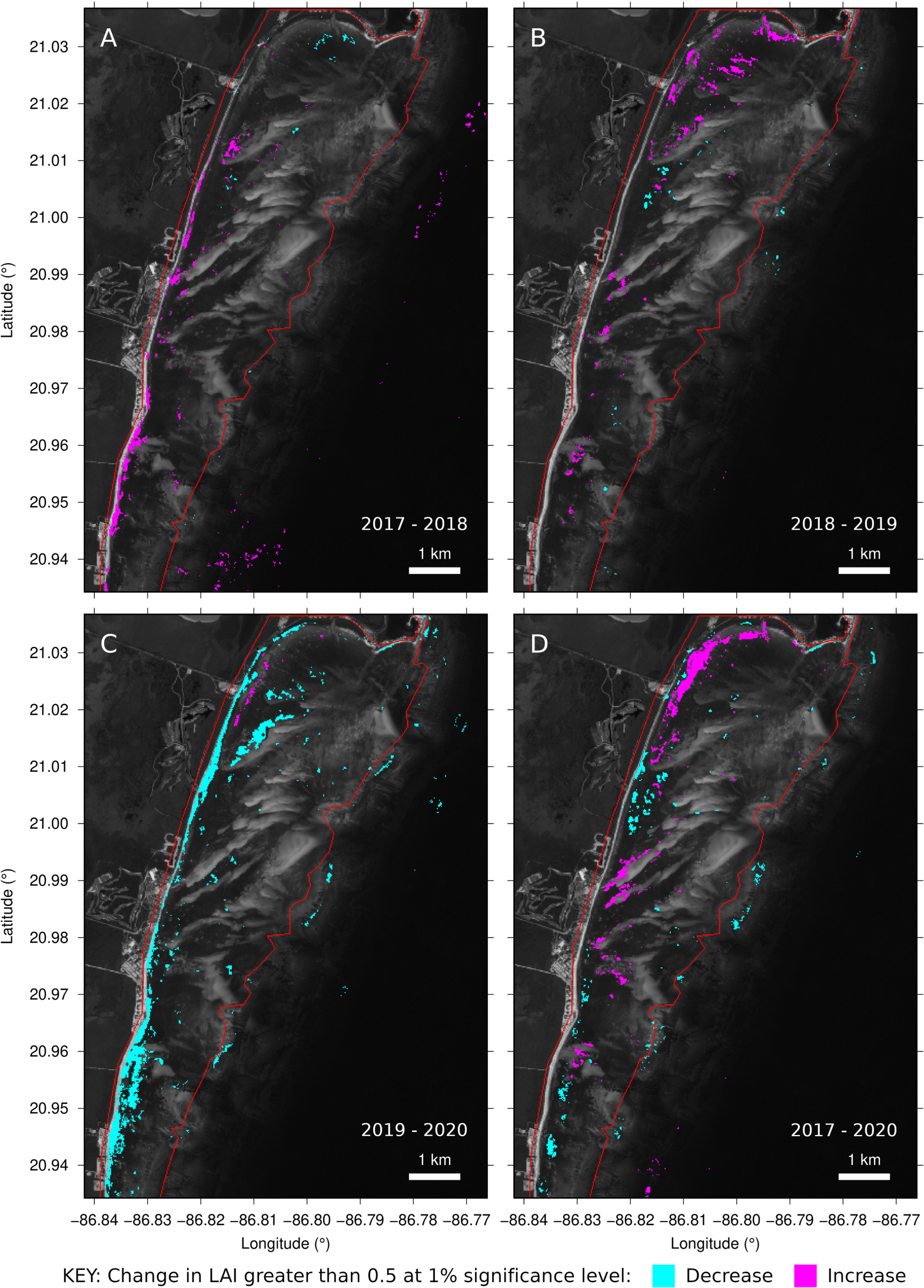
Figure 9. Changes in year-median LAI estimate in the northern Puerto Morelos lagoon. (A–C) For successive years from 2017. (D) Directly between years 2017 and 2020 ignoring 2018 and 2019. Red line shows lagoon area, changes outside of this relate to non-seagrass bottom types or factors.

The spatial pattern of change in any particular year-to-year comparison was very similar regardless of statistical significance level from 0.1% to 1% and for threshold changes in LAI of 0.1 to 0.5. Only when the significance level was reduced to 5% were excessive areas of “change” over deep water and other areas flagged (results not shown). Further, both the randomised tests and self-tests in regions of tile overlap identified virtually no changes at the 1% level, consistent with a meaningful change detection algorithm. This supports the interpretation that the changes identified are “real” in that they represent places where there was a systematic difference between the imagery from the years in question, although it does not confirm the basis of those differences.

Plotting individual image LAI estimates for one point over time (Figure 10B) shows the underlying data samples that contributed to the identified change year-to-year. Individual LAI estimates vary widely, with the most extreme outliers being due to unscreened clouds and cloud shadows (Figure 10, images 2 and 7). Despite this, variation trends are clearly visible, such as a higher year-median LAI estimate in 2019, which was statistically significant at the 1% level (Figure 10B). However, these identified changes may not be due to T. testudinum canopy LAI per se, because any apparent darkening of the reflectance may lead to an apparent LAI increase. Spatially, changes from 2019 to 2020 in the Puerto Morelos lagoon were dominated by an apparent decrease in estimated LAI along the shoreline (Figure 9D), whereas in previous years the tendency was an increase (Figures 9B,C). Almost certainly this change picked up by the analysis is from pelagic Sargassum collecting on the shoreline during 2018–2019. Data on beached Sargassum abundance in the area (García-Sánchez et al., 2020) mirrors almost exactly the LAI estimates (Figure 10C). The apparent decreases in the canopy LAI along the shoreline estimated from 2019 to 2020, may not only reflect the removal of the Sargassum deposits on the coast, but also the impact on the coastal seagrass meadows (van Tussenbroek et al., 2017).

FIGURE 10

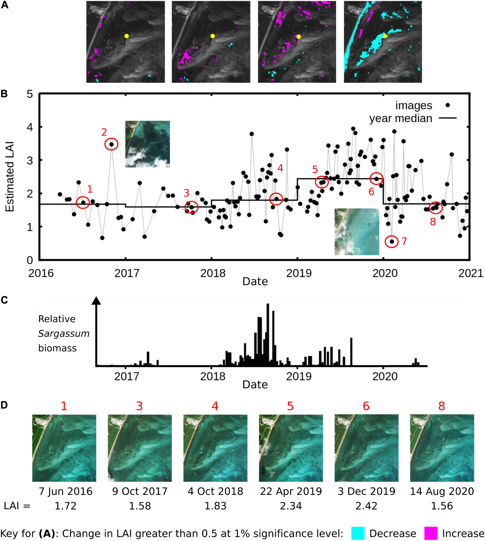
Figure 10. Detail of LAI estimation at one location (21.01747° N, –86.80708° W) in the northern Puerto Morelos lagoon. (A) Map of changes of greater than 0.5 LAI (p < 0.01) in successive year-median LAIs, starting at 2016–2017, etc. (B) Per-image LAI estimate and year median at the yellow point in (A), note the increase and decrease for 2019 are significant at the 1% level. (C) Sargassum beached biomass data for section of coastline in the area, adapted from García-Sánchez et al. (2020) and aligned with (B) by date. (D) RGB of atmospherically corrected images as highlighted in (B). Points numbered 2 and 7 in (B) are outliers due to cloud shadow and thin cloud, respectively.

The ability to detect the Sargassum in an environment of shallow dense seagrass canopies indicates the sensitivity of an analysis based on the entire image archive, and on the value of processing all images to an LAI time series. The influence of the Sargassum is clear due to the spatial pattern of the results and co-incidence with periods of known abundance in the time series. While in some Sentinel-2 images large mats of floating Sargassum are occasionally visible on the shoreline, in general, and especially over seagrasses, the Sargassum is not visible. The location shown in Figure 10 is actually quite far from the shoreline but appears to be systematically influenced by Sargassum even though this is not apparent in the original images (images 5 and 6 in Figure 10D look the same as the others). Sargassum deposited on the beaches breaks down rapidly and is dispersed into the lagoon as a function of local hydrodynamics and currents; this is likely what is being detected.

Excluding years 2018 and 2019, which were the most affected by Sargassum tides (García-Sánchez et al., 2020) gives a better synoptic view of changes in the T. testudinum canopy. Comparing years 2017 and 2020 (Figure 9D) reveals a spatial mix of increases and decreases which is consistent along the coast wherever seagrass is present. In another interpretation, whether the organic material is increased in Thalassia testudinum canopies, due to increases in seagrass productivity, macroalgal growth, or decomposing Sargassum is of less significance − the identified increase in “LAI” across the reef lagoon can be treated as a useful proxy of organic material, which may have an overall relevance to the progress of eutrophication or for monitoring processes that are happening in different parts of the lagoon. At the spatial scale of the entire coast this may be useful information for management.

The high variability in the individual image estimations of LAI (Figure 10) underlines the importance of careful interpretation, using multiple years of analysis, redundant data and statistical analyses. The variation is not entirely due to Sargassum presence, since it is largely absent in 2016 and 2017 − however, there are many other potential “noise” sources in the state of the water column, water surface or atmosphere. An analysis based on comparing single images, or fewer years, would have very little control with respect to this variation and could come to a false conclusion of change, particularly during periods of environmental disturbances. Classification or deep learning methods which rely on field survey training data are especially vulnerable. If, for example, training data lay in a location affected by Sargassum in a particular year, the consequence might be under-estimation of LAI propagated throughout the entire analysis.

Leaf Area Index-Depth Regime

Over the entire processed lagoon area the depth distribution of the highest estimated LAI areas was in good agreement with the expected upper limit from the oligotrophic field data of Enríquez et al. (2019) (Figure 11A, EOCH2019 line). LAIs greater than 3.5 were largely restricted to depths less than 2 m, in line with field characterisation of T. testudinum distribution. Combined with basic visual interpretation (Figure 4 and Supplementary Figures 3–13) the analysis would appear to have good capability to capture locations of high LAIs in shallow areas, which are the areas of the most significant below-ground carbon storage for this seagrass (Enríquez et al., 2019).

FIGURE 11

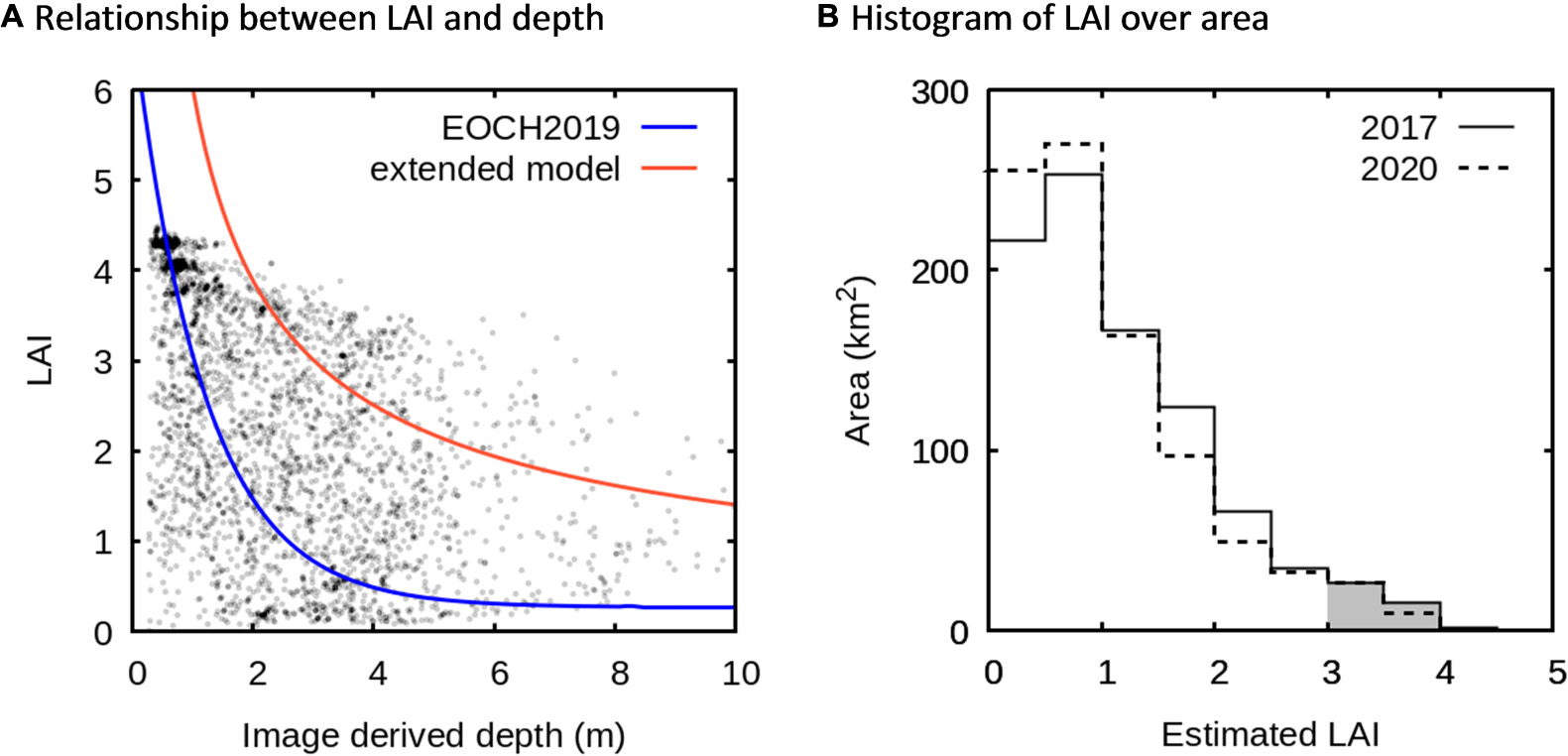
Figure 11. (A) Relative distribution of estimated LAI versus depth over the lagoon area (∼825 km²) for 2017. Data has been evenly stratified by LAI in bins of 0.5, to show the relative occurrence of LAIs at specific depths. Lines are upper limits of LAI from local field survey (EOCH2019, Eq. 1), and the extended model (Eq. 2) (see Figure 3). (B) Histogram showing areal cover as a function of LAI for 2017 and 2020. Shaded area is LAI > 3 and represents 43.1 km² for 2019 and 36.4 km² for 2020.

Leaf area index values less than 3.5 were found at a wide range depths encompassing both the oligotrophic EOCH2019 model and the extended model (Figure 11A). As expected, some areas are under-colonised due to disturbance processes, but also, seagrass densities above the oligotrophic climax colonisation expected at specific depths do occur. LAI values above even the extended model were mainly observed in the center of large seagrass patches (Figure 4D). This could be due to the accumulation of organic matter in the sediment, as any apparent darkening of the reflectance may lead, as indicated previously, to an apparent LAI increase. However, the extended model may also underestimate the highest LAIs that can be achieved. Field data at a site near the back-reef estimated an LAI value of 4.73 in a depth of 2.5 m, corresponding to “above the extended model” (the red area in Figures 3A, 4D). This site, “Limones,” is located in front of the largest coastal resort, the Moon Palace hotel (20.98956° 86.79894° W), and had sediment organic matter content of 3.8%, above the threshold for oligotrophic environments of 3.0% (Morse et al., 1987; Enríquez et al., 2001), but not high enough to affect LAI determinations through sediment darkening. More in situ work to characterise the upper bounds of LAI with depth may be required.

With respect to seagrass abundance at regional scale, for 2017 and 2020 the total area of dense canopy (estimated LAI > 3) was very similar and comprised less than 5% of the delimited lagoon area along the entire coast, being a total of 43.1 and 36.4 km², respectively (Figure 11B). For 2018 and 2019 this estimate was higher at 70 and 66 km², but Figure 10 suggests these higher values are mainly due to pelagic Sargassum debris dispersed from the beach into the lagoon. So, ignoring 2018 and 2019 and considering only 2017 and 2020 (years when reported Sargassum was minimal, cf. García-Sánchez et al., 2020) the estimated area of dense canopy (LAI > 3) exhibited a net decrease of 6.7 km². However, according to the statistical test in the change detection analysis only a net area of 1.7 km² represented a statistically significant decrease of 0.1 or more in areas of dense canopy (LAI > 3) (p < 0.01). The safest conclusion is that, between 2017 and 2020, there has been negligible change in the areal cover of high LAI canopies. Note that the seagrass platform characterised in Enríquez et al. (2019) was removed by hurricane Wilma in 2005, and that coastal seagrass meadows were previously affected by the Sargassum tides in 2014 and 2015 (van Tussenbroek et al., 2017). The time scale analysed here was too short to detect seagrass changes at the decadal scales required to understand these impacts.

A reasonable estimate for the coverage of high LAI canopies (LAI > 3) is the average of 2017 and 2020, giving ∼40 km² in 900 km² of shallow coastal lagoon. Guimarais et al. (2021) provided a figure of 576 km² of “seagrass meadows” in the Mexican Caribbean, which in our analysis is the area of estimated LAI greater than 0.7 (563 km²). This is consistent with a presence-absence threshold for Thalassia testudinum since in mixed canopy other macrophytes may contribute around 0.5 to LAI (Supplementary Figure 1). Nevertheless, in terms of the function of the canopy as a carbon sink 576 km² would seem too large a figure, since the accumulation of below ground biomass is only significant for dense canopies located at the shoreline (Enríquez et al., 2019), which in our results comprise at most only 5% of the total “seagrass meadow” area.

Large-Scale Patterns Along the Coastline

Variation in Seagrass Cover and Association With Freshwater Outflows

The relative area covered by different canopy densities (Figure 11B) differed over the eleven sites of interest (Figure 12; Table 1 and Supplementary Figures 3–13). Three sites had particularly large areas of relatively bare substrate (50% area of LAI < 1, Figure 12A): the Isla Mujeres site north of Cancun (IM) and two sites in the Sian Ka’an Biosphere reserve, the bays, Bahía de la Ascensión (AN) and Bahía del Espíritu Santo (ESN). Areal coverage by dense canopies (estimated LAI > 3) was greater in the northern part of the coastline, especially in Punta Nizuc and in the Puerto Morelos marine park (Figure 12B). Although on average sites in the south had less dense canopies (Figure 12), this was also true of the northern-most site (IM) and there was not a very consistent north-south gradient in relative canopy cover. The three sites of the Sian Ka’an Biosphere reserve were very diverse in terms of seagrass colonisation, from high values in San Miguel-Zamak (SMZ) to the lowest seagrass presence the bays AN and ESN (Figure 12).

FIGURE 12

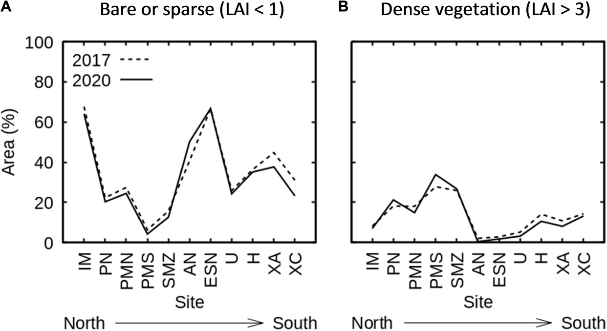
Figure 12. Relative area of (A) bare substrate or sparse canopies (estimated LAI < 1) and (B) dense canopies (estimated LAI > 3) found at the eleven sites of interest, ordered from north to south.

The previous conclusion of relatively little overall change from 2017 to 2020 was also observed at the individual sites. One notable exception is the Bahía de la Ascensión site (AN) which was predominantly sparse canopy (LAI < 1) or bare substrate, and Figure 12A suggests these sparse canopies thinned out even more between 2017 and 2020. In fact, this is clearly visually apparent as a trend in the successive year results across the whole bay (of which the AN site is only part) (Supplementary Figure 14). Rainfall in the region has been systematically high since 2013, by up to 2% compared to the previous 10 years (GM, 2021 and Supplementary Figure 15). Seagrass meadows in these bays are known to be influenced by freshwater outflows, particularly in the rainy season (Medina-Gómez et al., 2016), so this may be a causal factor in the apparent trajectory of canopy decrease.

North-South Seagrass Variation Associated With a Gradient of Anthropogenic Impact

Interestingly, the LAI-depth regime exhibited a clear north to south trend of decreasing canopy LAI as a function of depth (Figure 13) whereas the previous simple quantification of relative sparse or dense canopy area in itself did not show such a trend (Figure 12). Figure 13 is restricted to the areas where LAI was greater than 2 to avoid the influence of non-Thalassia testudinum macrophytes in very sparse areas, but the pattern is the same if all LAIs or only LAIs greater than 3 are included. This supports the utility of the LAI-depth regime as a metric which is able to compare sites with different levels of seagrass colonisation − that is, when LAI is viewed as function of depth underlying similarities or trends may be more apparent.

FIGURE 13

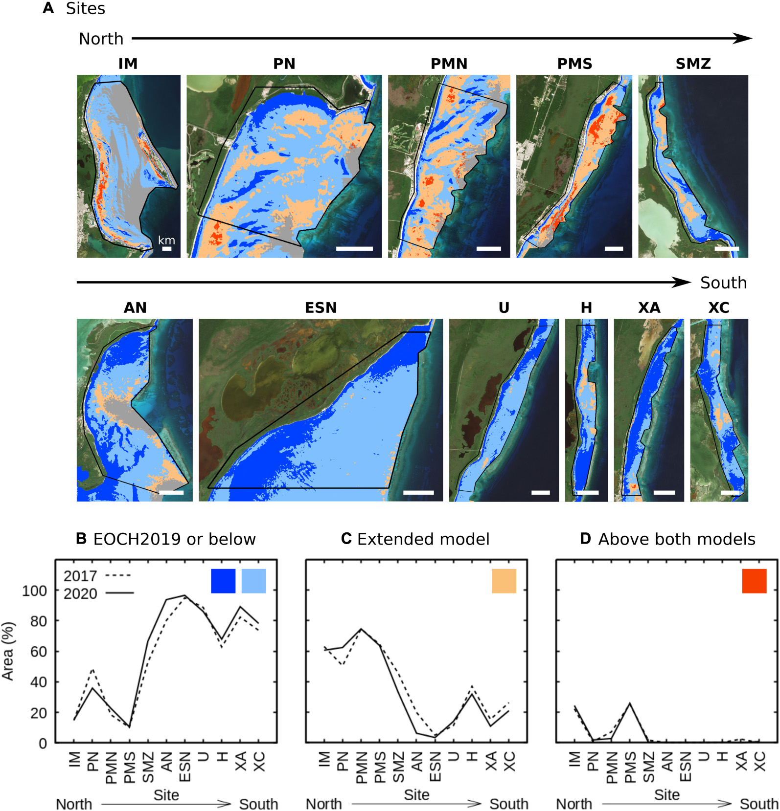
Figure 13. Relative areas of different LAI-depth regimes, restricted to canopies of LAI > 2, found at (A) the eleven sites of interest. Colours indicate which categories are included corresponding to Figure 3. (B) Relative area where estimated LAI was less than or consistent with EOCH2019 at the depth of occurrence, (C) where estimated LAI corresponded to the range defined by the extended model, (D) where estimated LAI was greater than expected by either model.

The trend of denser canopies in the north part of the coast mirrors the pattern of touristic infrastructure developed since the 1970s, and so is consistent with the interpretation of an eutrophication impact arising from coastal development. In particular, the most developed locations, the lagoon area immediately offshore from the town of Puerto Morelos (PMS) and the Isla Mujeres site (IM) close to the city of Cancún, had substantial relative areas with LAI estimates above the upper bounds expected at that depth by even the extended model (Figure 13C). The interpretation of nutrient driven change is supported by the lack of tertiary sewage treatment for the large urban and tourist resort population in this area. A number of studies have documented nutrient concentrations in the Mexican Caribbean higher than expected for oligotrophic coastal ecosystems, particularly in the north (Carruthers et al., 2005; Mutchler et al., 2010; Hernández-Terrones et al., 2011, 2015; Almazán-Becerril et al., 2014; Null et al., 2014; Pérez-Gómez et al., 2020). Some studies have provided evidence that ground water discharges are the primary source of the nutrient enrichment (Mutchler et al., 2010; Hernández-Terrones et al., 2011, 2015; Null et al., 2014). Stable isotopes (δ¹⁵N) indicate the assimilation of sewage by different organisms including T. testudinum (Carruthers et al., 2005; Pérez-Gómez et al., 2020). Based on a field survey data review, Guimarais et al. (2021) also found a northward deterioration in the coastal ecosystem state, deduced from several metrics including the state of coral reefs and the presence of “climax” Thalassia testudinum habitats. However, data on the pattern of eutrophication along the coast was not very consistent, 124 samples at various locations over 1991 to 2018 did not show a clear north-south gradient (Guimarais et al., 2021) and were inconsistent even at local scales. Our in situ descriptions have confirmed higher sediment nutrient concentrations associated with locations characterised by the extended model (Figure 3C, See section “Leaf Area Index-Depth Regime”). This data supports the hypothesis that increases in LAI could be considered the response of the seagrass to an influx of nutrients from urban and touristic development of the coast. The trends shown in Figure 13 suggest remote-sensing proxies could be useful complementary indicators to reveal these large-scale patterns, and may be worthy of further investigation.

The gradient in LAI-regime, which showed that canopies in environments of known anthropogenic impacts tend to be denser, draws into question the assumption that seagrass regression is the only change consistent with environmental deterioration of seagrass habitats (e.g., Orth et al., 2006; Waycott et al., 2009). The 5-year time period of our analysis was too short to demonstrate any temporal effect of coastal development. However, if our interpretation is correct, the rapid coastal development since the 1970s, predominantly in the north, implies that the current south to north gradient in LAI-depth regime would be expected to be mirrored by a change over time in the northern part of the coast, but at decadal scales. A previous remote sensing analysis using a different methodology did suggest a potential increase in canopy density in the northern part of the Puerto Morelos lagoon from 1992 to 2011 (Supplementary Figure 16). A future priority is to extend the new analysis method historically using Landsat and SPOT archives, possibly with images grouped in 5 year steps to provide sufficient sample replicates for statistical analysis.

Detection of Sargassum

As a final example of the many possible uses of the full dataset arising from this analysis, the area of statistically significant changes in estimated LAI was interpreted as a proxy for Sargassum impact at the eleven sites of interest (Figure 14). The rationale was that an increase in 2017 to 2018 and/or 2018 to 2019 corresponding to a decrease in 2019 to 2020 would be largely attributable to changes associated with Sargassum presence and removal. In fact, over the eleven sites the area of increase and subsequent area of decrease was highly correlated and numerically similar (Figure 14). This pattern indicates “something” being absent in 2017, present in 2018 and 2019, and then absent in 2020. Since this coincides with the known incidence of pelagic Sargassum tides in 2018 and 2019 it further supports the interpretation developed throughout this paper of the Sargassum effect in 2018 and 2019. Two corollaries to this are: (1) the influence of Sargassum on the LAI results was only deducible by careful interpretation of a multi-year analysis, showing the importance of redundant data to interpret apparent changes; and (2) at least in year-to-year time scales, the method provides a proxy for Sargassum incidence despite the confounding effect of heterogeneous bottom reflectances in these shallow lagoons. Since monitoring Sargassum inputs along ∼400 km of coastline is impractical by physical surveys, this proxy may find use in future years. The current analysis indicates that the areas with the least incursion of pelagic Sargassum were the far north, far south, and the ESN site which is a south-west facing section of coastline at the edge of the large “Bahía del Espíritu Santo” bay. These results are broadly consistent with an estimation of Sargassum occurrence in the open sea from 2016 to 2020 using Landsat 8 (Chávez et al., 2020), although our analysis, which identifies lagoonal material, implies a greater occurrence in southern locations such as Huache (site H).

FIGURE 14

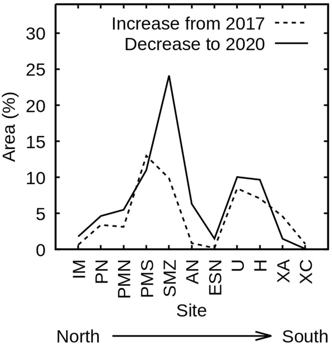
Figure 14. Effect of Sargassum on LAI estimates at the sites of interest ordered north to south. Dashed line is net area with increase in estimated LAI greater than 0.5 (p < 0.01) from 2017 to 2018 and 2018 to 2019 summed. Solid line is net area decrease greater than 0.5 (p < 0.01) 2019 to 2020.

Conclusion

The aim of this study was to characterise the LAI-depth distribution of Thalassia testudinum canopies in the coastal reef lagoon of the entire Eastern Mexican Caribbean, an area of 900 km². At a technical level, various interpretations applied to the results implies this has been achieved to a satisfactory accuracy. Visual interpretation, in situ LAI point data, ICESat-2 bathymetry data, and previous estimates of canopy area, are all consistent with the data layers produced by the analysis. A slight tendency to overestimate depth over dark benthos and vice-versa, to a level of around ± 0.5 m, is within the tolerances required for our analysis. Year-to-year change detection reveals localised canopy extension and retraction, but is also dominated by incursion of pelagic Sargassum in 2018 and 2019. That these apparent changes are due to Sargassum is supported by several angles of interpretation, including comparison to in situ data. Overall, at the scale of the analysis, we conclude there was no significant change in seagrass abundance over the period 2016–2020. This is largely expected considering the short period of time characterised, and that previous to the period of analysis other phenomena had caused major impacts on these meadows: hurricane Wilma in October 2005 and the first massive Sargassum tides in the area which occurred in 2014 and 2015. Thalassia testudinum is a slow growing species that requires recovery times longer than 4–5 years.

The consistency of the results, especially between 2017 and 2020, indicate that general conclusions can made about the depth and density distribution of Thalassia testudinum canopies. The estimated total area of seagrass canopies along the Mexican Caribbean coast is consistent with previous estimates of ∼580 km², but only ∼40 km² consists of the dense canopies (LAI > 3) which are the primary contributors to below-ground carbon storage. Although the relative area of the seagrass canopies varies from site to site, when considered as a function of depth, the distribution of canopy density mirrors an established north-south gradient in anthropogenic environmental impact. We propose this metric can be used as a proxy for characterising environmental status of tropical seagrass meadows at large scales (100s km). Importantly, the pattern of the north-south gradient described is such that canopies at specific depths are denser in more impacted environments, and this applies even when only dense canopies of LAIs greater than 2 or 3 are considered. Although our study did not aim to identify a causal mechanism, there is experimental evidence that nutrient enrichment stimulates leaf growth and increases in leaf area and biomass in Thalassia testudinum. Hence, our hypothesis is that sustained increases in nutrient availability stimulate canopy growth to densities beyond that which would normally occur in the oligotrophic climax habitat.

In our results the LAI-depth regime mirrors environmental impact over a spatial gradient; the hypothesis would be further supported by demonstration over a temporal gradient. This would be the next step for investigation, although leveraging historical satellite image sources over decadal time scales offers challenges to the methodology; the frequency and spatial resolution of Sentinel-2 acquisitions are superior to previous generations of sensor. In any case, one consequence implied by our results is that environmental deterioration may be indicated, at least initially, by an increase in seagrass canopy density. This possibility may need to be further evaluated in the context of management and monitoring. The status of seagrass habitats may also be useful as an early bio-indicator of the environmental status of associated reef habitats. The complex benthos of coral reefs is a challenge for remote sensing of “reef health”; quantification of seagrass LAI and depth may be a more achievable objective with greater sensitivity to the initial stages of environmental change.

Data Availability Statement

The datasets presented in this article are not readily available because aspects of them are dynamically generated and interpretation may not be straightforward. Nevertheless, interested parties are welcome to contact us. Requests to access the datasets should be directed to JH, j.d.hedley@numopt.com.

Author Contributions

SE and JH designed the research, analysed the results, and wrote the manuscript. JH developed the remote sensing analysis. RV-O performed the field work. All authors reviewed the manuscript.

Funding

This research leading to these results has received funding from the Mexican CONACYT research project (Conv-CB-2009: 129880) to SE, and the European Union 7th Framework programme (P7/2007-2013) under grant agreement No. 244161 to SE. This manuscript is part of the fulfillment requirements of the Ph.D. degree of RV-O in the postgraduate program of Ciencias del Mar y Limnología (PCMyL) of the Universidad Nacional Autónoma de México (UNAM). This program is also acknowledged for providing 4 years of a CONACYT fellowship to support the Ph.D. degree of RV-O. All map images in this manuscript contain modified Copernicus Sentinel data (2016–2020).

Conflict of Interest

JH is employed by Numerical Optics Ltd.

The remaining authors declare that the research was conducted in the absence of any commercial or financial relationships that could be construed as a potential conflict of interest.

Publisher’s Note

All claims expressed in this article are solely those of the authors and do not necessarily represent those of their affiliated organizations, or those of the publisher, the editors and the reviewers. Any product that may be evaluated in this article, or claim that may be made by its manufacturer, is not guaranteed or endorsed by the publisher.

Supplementary Material

The Supplementary Material for this article can be found online at: https://www.frontiersin.org/articles/10.3389/fmars.2021.733169/full#supplementary-material

References

Agawin, N. S. R., and Duarte, C. M. (2002). Evidence of direct particle trapping by a tropical seagrass meadow. Estuaries 25, 1205–1209. doi: 10.1007/BF02692217

CrossRef Full Text | Google Scholar

Almazán-Becerril, A., Abundes, M., Francisco, V., López, I., Ramos, L., Álvarez-Filip, L., et al. (2014). Programa de Monitoreo Biológico (PROMOBI) 2014. Final Report. Mexico, MX: CONANP.

Google Scholar

Bricker, S. B., Clement, C. G., Pirhalla, D. E., Orlando, S. P., and Farrow, D. R. G. (1999). National Estuarine Eutrophication Assessment: Effects of Nutrient Enrichment in the Nation’s Estuaries. Silver Spring, MD: NOAA, National Ocean Service, Special Projects Office and the National Centers for Coastal Ocean Science, 71.

Google Scholar

Cabaço, S., Apostolaki, E. T., García−Marín, P., Gruber, R., Hernández, I., Martínez−Crego, B., et al. (2013). Effects of nutrient enrichment on seagrass population dynamics: evidence and synthesis from the biomass–density relationships. J. Ecol. 101, 1552–1562. doi: 10.1111/1365-2745.12134

CrossRef Full Text | Google Scholar

Cabaço, S., Santos, R., and Duarte, C. M. (2008). The impact of sediment burial and erosion on seagrasses: a review. Estuar. Coast. Shelf Sci. 79, 354–366. doi: 10.1016/j.ecss.2008.04.021

CrossRef Full Text | Google Scholar

CARICOMP (1994). CARICOMP Methods Manual-Level I. Manual of Methods for Mapping and Monitoring of Physical and Biological Parameters in the Coastal Zone of the Caribbean. Mona: CARICOMP Data Management Centre, University of the West Indies.

Google Scholar

Carruthers, T. J. B., van Tussenbroek, B. I., and Dennison, W. C. (2005). Influence of submarine springs and wastewater on nutrient dynamics of Caribbean seagrass meadows. Estuar. Coast. Shelf Sci. 64, 191–199. doi: 10.1016/j.ecss.2005.01.015

CrossRef Full Text | Google Scholar

Casal, G., Hedley, J. D., Monteys, X., Harris, P., Cahalane, C., and McCarthy, T. (2020). Satellite-derived bathymetry in optically complex waters using a model inversion approach and Sentinel-2 data. Estuar. Coast. Shelf Sci. 241:106814. doi: 10.1016/j.ecss.2020.106814

CrossRef Full Text | Google Scholar

Chávez, V., Uribe-Martínez, A., Cuevas, E., Rodriguez-Martinez, R., Francisco, V., Estevez, M., et al. (2020). Massive influx of pelagic Sargassum spp. on the coasts of the Mexican Caribbean 2014-2020: challenges and opportunities. Water 12:2908. doi: 10.3390/w12102908

CrossRef Full Text | Google Scholar

Chollett, I., Mumby, P. J., Müller-Karger, F. E., and Hu, C. (2012). Physical environments of the Caribbean Sea. Limnol. Oceanogr. 57, 1233–1244. doi: 10.4319/lo.2012.57.4.1233

CrossRef Full Text | Google Scholar

Coronado, C., Candela, J., Iglesias-Prieto, R., Sheinbaum, J., López, M., and Ocampo-Torres, F. J. (2007). On the circulation in the Puerto Morelos fringing reef lagoon. Coral Reefs 26, 149–163. doi: 10.1007/s00338-006-0175-9

CrossRef Full Text | Google Scholar

Cortés, J., Oxenford, H. A., van Tussenbroek, B. I., Jordán-Dahlgren, E., Cróquer, A., Bastidas, C., et al. (2019). The CARICOMP network of Caribbean marine laboratories (1985–2007): history, key findings, and lessons learned. Front. Mar. Sci. 5:519. doi: 10.3389/fmars.2018.00519

CrossRef Full Text | Google Scholar

Costanza, R., d’Arge, R., de Groot, R., Farber, S., Grasso, M., Hannon, B., et al. (1997). The value of the world’s ecosystem services and natural capital. Nature 387, 253–260. doi: 10.1038/387253a0

CrossRef Full Text | Google Scholar

Cunha, A. H., Santos, R. P., Gaspar, A. P., and Bairros, M. F. (2005). Seagrass landscape-scale changes in response to disturbance created by the dynamics of barrier-islands: a case study from Ría Formosa (Southern Portugal). Estuar. Coast. Shelf Sci. 64, 636–644. doi: 10.1016/j.ecss.2005.03.018

CrossRef Full Text | Google Scholar

Duarte, C. M., and Chiscano, C. L. (1999). Seagrass biomass and production: a reassessment. Aquat. Bot. 65, 159–174. doi: 10.1016/s0304-3770(99)00038-8

CrossRef Full Text | Google Scholar

Duarte, C. M., Middelburg, J. J., and Caraco, N. (2005). Major role of marine vegetation on the oceanic carbon cycle. Biogeosciences 2, 1–8. doi: 10.5194/bg-2-1-2005

CrossRef Full Text | Google Scholar

Egbert, G. D., and Erofeeva, S. Y. (2002). Efficient inverse modeling of barotropic ocean tides. J. Atmos. Ocean. Technol. 19, 183–204. doi: 10.1175/1520-04262002019<0183:EIMOBO<2.0.CO;2

CrossRef Full Text | Google Scholar

Enríquez, S., Marbá, N., Duarte, C. M., van Tussenbroek, B., and Reyes, G. (2001). Effects of seagrass (Thalassia testudinum) on sediment redox. Mar. Ecol. Prog. Ser. 219, 149–158. doi: 10.3354/meps219149

CrossRef Full Text | Google Scholar

Enríquez, S., Olivé, I., Cayabyab, N., and Hedley, J. D. (2019). Structural complexity governs seagrass acclimatization to depth with relevant consequences for meadow production, macrophyte diversity and habitat carbon storage capacity. Sci. Rep. 9:14657. doi: 10.1038/s41598-019-51248-z

PubMed Abstract | CrossRef Full Text | Google Scholar

Enríquez, S., and Pantoja-Reyes, N. I. (2005). Form-function analysis of the effect of canopy morphology on leaf self-shading in the seagrass Thalassia testudinum. Oecologia 145, 235–243. doi: 10.1007/s00442-005-0111-7

PubMed Abstract | CrossRef Full Text | Google Scholar

Enríquez, S., and Schubert, N. (2014). Direct contribution of the seagrass Thalassia testudinum to lime mud production. Nat. Commun. 5:4835. doi: 10.1038/ncomms4835

PubMed Abstract | CrossRef Full Text | Google Scholar

Fonesca, M. S., and Cahalan, J. A. (1992). A preliminary evaluation of wave attenuation by four species of seagrass. Estuar. Coast. Shelf Sci. 35, 565–576. doi: 10.1016/S0272-7714(05)80039-3

CrossRef Full Text | Google Scholar

Fourqurean, J. W., Duarte, C. M., Kennedy, H., Marbà, N., Holmer, M., Mateo, M. A., et al. (2012). Seagrass ecosystems as a globally significant carbon stock. Nat. Geosci. 5, 505–509. doi: 10.1038/ngeo1477

CrossRef Full Text | Google Scholar

Fourqurean, J. W., Zieman, J. C., and Powell, G. V. N. (1992). Phosphorus limitation of primary production in Florida Bay: evidence from C:N:P ratios of the dominant seagrass Thalassia testudinum. Limnol. Oceanogr. 37, 162–171. doi: 10.4319/lo.1992.37.1.0162

CrossRef Full Text | Google Scholar

Frankovich, T. A., and Fourqurean, J. W. (1997). Seagrass epiphyte loads along a nutrient availability gradient, Florida Bay, USA. Mar. Ecol. Prog. Ser. 159, 37–50. doi: 10.3354/meps159037

CrossRef Full Text | Google Scholar

Gacia, E., Granata, T. C., and Duarte, C. M. (1999). An approach to measurement of particle flux and sediment retention within seagrass (Posidonia oceanica) meadows. Aquat. Bot. 65, 255–268. doi: 10.1016/S0304-3770(99)00044-3

CrossRef Full Text | Google Scholar

Gapper, J. J., El-Askary, H., Linstead, E., and Piechota, T. (2019). Coral reef change detection in remote Pacific islands using support vector machine classifiers. Remote Sens. 11:1525. doi: 10.3390/rs11131525

CrossRef Full Text | Google Scholar

García-Sánchez, M., Graham, C., Vera, E., Escalante-Mancera, E., Álvarez-Filip, L., and van Tussenbroek, B. I. (2020). Temporal changes in the composition and biomass of beached pelagic Sargassum species in the Mexican Caribbean. Aquat. Bot. 167:103275. doi: 10.1016/j.aquabot.2020.103275

CrossRef Full Text | Google Scholar

GEF (2010). Coral Reef Targeted Research and Capacity Building for Management. Available online at: https://www.thegef.org/project/coral-reef-targeted-research-and-capacity-building-management (accessed September 24, 2021).

Google Scholar

Gillanders, B. M. (2006). “Seagrasses, fish and fisheries,” in Seagrasses: Biology, Ecology and Conservation, eds A. W. D. Larkum, R. J. Orth, and C. M. Duarte (Dordrecht: Springer), 503–536. doi: 10.1007/978-1-4020-2983-7_21

CrossRef Full Text | Google Scholar

GM (2021). Historical Average Rainfall by State (Precipitación Media Histórica Por Entidad Federativa). Mexican Government Report. Available online at: https://www.gob.mx (accessed September 24, 2021).

Google Scholar

González-Barrios, F. J., and Álvarez-Filip, L. (2018). A framework for measuring coral species-specific contribution to reef functioning in the Caribbean. Ecol. Indic. 95, 877–886. doi: 10.1016/j.ecolind.2018.08.038

CrossRef Full Text | Google Scholar

Grech, A., Coles, R., and Marsh, H. (2011). A broad-scale assessment of the risk to coastal seagrasses from cumulative threats. Mar. Policy 35, 560–567. doi: 10.1016/j.marpol.2011.03.003

CrossRef Full Text | Google Scholar

Guimarais, M., Zúñiga-Ríos, A., Cruz-Ramírez, C. J., Chávez, V., Odériz, I., van Tussenbroek, B. I., et al. (2021). The conservational state of coastal ecosystems on the Mexican Caribbean coast: environmental guidelines for their management. Sustainability 13:2738. doi: 10.3390/su13052738

CrossRef Full Text | Google Scholar

Hamylton, S. M., Hedley, J. D., and Beaman, R. J. (2015). Derivation of high-resolution bathymetry from multispectral satellite imagery: a comparison of empirical and optimisation methods through geographical error analysis. Remote Sens. 7, 16257–16273. doi: 10.3390/rs71215829

CrossRef Full Text | Google Scholar

Hedley, J. D. (2008). A three-dimensional radiative transfer model for shallow water environments. Opt. Expr. 16, 21887–21902. doi: 10.1364/OE.16.021887

PubMed Abstract | CrossRef Full Text | Google Scholar

Hedley, J. D., and Enríquez, S. (2010). Optical properties of canopies of the tropical seagrass Thalassia testudinum estimated by a three-dimensional radiative transfer model. Limnol. Oceanogr. 55, 1537–1550. doi: 10.4319/lo.2010.55.4.1537

CrossRef Full Text | Google Scholar

Hedley, J. D., Harborne, A. R., and Mumby, P. J. (2005). Simple and robust removal of sun glint for mapping shallow-water benthos. Int. J. Rem. Sens. 26, 2107–2112. doi: 10.1080/01431160500034086

CrossRef Full Text | Google Scholar

Hedley, J. D., McMahon, K., and Fearns, P. (2014). Seagrass canopy photosynthetic response is a function of canopy density and light environment: a model for Amphibolis griffithii. PLoS One 9:e111454. doi: 10.1371/journal.pone.0111454

PubMed Abstract | CrossRef Full Text | Google Scholar

Hedley, J. D., Roelfsema, C., Brando, V., Giardino, C., Kutser, T., Phinn, S., et al. (2018). Coral reef applications of Sentinel-2: coverage, characteristics, bathymetry and benthic mapping with comparison to Landsat 8. Rem. Sens. Environ. 216, 598–614. doi: 10.1016/j.rse.2018.07.014

CrossRef Full Text | Google Scholar

Hedley, J. D., Roelfsema, C., Koetz, B., and Phinn, S. (2012). Capability of the Sentinel 2 mission for tropical coral reef mapping and coral bleaching detection. Rem. Sens. Environ. 120, 145–155. doi: 10.1016/j.rse.2011.06.028

CrossRef Full Text | Google Scholar

Hedley, J. D., Roelfsema, C., and Phinn, S. R. (2009). Efficient radiative transfer model inversion for remote sensing applications. Rem. Sens. Environ. 113, 2527–2532. doi: 10.1016/j.rse.2009.07.008

CrossRef Full Text | Google Scholar

Hedley, J. D., Russell, B., Randolph, K., and Dierssen, H. (2016). A physics-based method for the remote sensing of seagrasses. Rem. Sens. Environ. 174, 134–147. doi: 10.1016/j.rse.2015.12.001

CrossRef Full Text | Google Scholar

Hedley, J. D., Russell, B. J., Randolph, K., Pérez-Castro, M. A., Vásquez-Elizondo, R. M., Enríquez, S., et al. (2017). Remote sensing of seagrass leaf area index and species: the capability of a model inversion method assessed by sensitivity analysis and hyperspectral data of Florida Bay. Front. Mar. Sci. 4:362. doi: 10.3389/fmars.2017.00362

CrossRef Full Text | Google Scholar

Hernández-Delgado, E. A., Toledo-Hernández, C., Ruíz-Díaz, C. P., Gómez-Andújar, N., Medina-Muñiz, J. L., Canals-Silander, M. F., et al. (2020). Hurricane impacts and the resilience of the invasive sea vine, Halophila stipulacea: a case study from Puerto Rico. Estuaries Coasts 43, 1263–1283. doi: 10.1007/s12237-019-00673-4

CrossRef Full Text | Google Scholar

Hernández-Terrones, L., Rebolledo-Vieyra, M., and Merino-Ibarra, M. (2011). Groundwater pollution in a karstic region (NE Yucatan): baseline nutrient content and flux to coastal ecosystems. Water Air Soil Pollut. 218, 517–528. doi: 10.1007/s11270-010-0664-x

CrossRef Full Text | Google Scholar

Hernández-Terrones, L. M., Null, K. A., Ortega-Camacho, D., and Paytan, A. (2015). Water quality assessment in the Mexican Caribbean: impacts on the coastal ecosystem. Cont. Shelf Res. 102, 62–72. doi: 10.1016/j.csr.2015.04.015

CrossRef Full Text | Google Scholar

Ilori, C. O., and Knudby, A. (2020). An approach to minimize atmospheric correction error and improve physics-based satellite-derived bathymetry in a coastal environment. Remote Sens. 12:2752. doi: 10.3390/rs12172752

CrossRef Full Text | Google Scholar

Kennedy, H., Beggins, J., Duarte, C. M., Fourqurean, J. W., Holmer, M., Marba, N., et al. (2010). Seagrass sediments as a global carbon sink: isotopic constraints. Glob. Biogeochem. Cycles 24:GB4026. doi: 10.1029/2010GB003848

CrossRef Full Text | Google Scholar

Knudby, A., and Nordlund, L. (2011). Remote sensing of seagrasses in a patchy multi-species environment. Int. J. Rem. Sens. 32, 2227–2244. doi: 10.1080/01431161003692057

CrossRef Full Text | Google Scholar

Kutser, T., Miller, I., and Jupp, D. L. B. (2002). “Mapping coral reef benthic habitat with a hyperspectral space borne sensor,” in Proceedings of the Ocean Optics XVI, 18–22 November 2002, Santa Fe, NM, 1–14.

Google Scholar

Kutser, T., Miller, I. R., and Jupp, D. L. B. (2006). Mapping coral reef benthic substrates using hyperspectral space-borne images and spectral libraries. Estuar. Coast. Shelf Sci. 70, 449–460. doi: 10.1016/j.ecss.2006.06.026

CrossRef Full Text | Google Scholar

Kutser, T., Vahtmäe, E., and Praks, J. (2009). A sun glint correction method for hyperspectral imagery containing areas with non-negligible water leaving NIR signal. Remote Sens. Environ. 113, 2267–2274. doi: 10.1016/j.rse.2009.06.016

CrossRef Full Text | Google Scholar

Lapointe, B. E. (1997). Nutrient thresholds for bottom-up control of macroalgal blooms on coral reefs in Jamaica and southeast Florida. Limnol. Oceanogr. 42(5 Pt 2), 1119–1131. doi: 10.4319/lo.1997.42.5_part_2.1119

CrossRef Full Text | Google Scholar

Lee, Z., Carder, K. L., Mobley, C. D., Steward, R. G., and Patch, J. S. (1998). Hyperspectral remote sensing for shallow waters. I. A semianalytical model. Appl. Opt. 37, 6329–6338. doi: 10.1364/AO.37.006329

PubMed Abstract | CrossRef Full Text | Google Scholar

Lee, Z., Carder, K. L., Mobley, C. D., Steward, R. G., and Patch, J. S. (1999). Hyperspectral remote sensing for shallow waters: 2. Deriving bottom depths and water properties by optimization. Appl. Opt. 38, 3831–3843. doi: 10.1364/AO.38.003831

PubMed Abstract | CrossRef Full Text | Google Scholar

Lyons, M. B., Roelfsema, C. M., and Phinn, S. R. (2013). Towards understanding temporal and spatial dynamics of seagrass landscapes using time-series remote sensing. Estuar. Coast. Shelf Sci. 120, 42–53. doi: 10.1016/j.ecss.2013.01.015

CrossRef Full Text | Google Scholar

Martínez-Crego, B., Vergés, A., Alcoverro, T., and Romero, J. (2008). Selection of multiple seagrass indicators for environmental biomonitoring. Mar. Ecol. Prog. Ser. 261, 93–109. doi: 10.3354/meps07358

CrossRef Full Text | Google Scholar

Medina-Gómez, I., Madden, C. J., Herrera-Silveira, J., and Kjerfve, B. (2016). Response of Thalassia testudinum morphometry and distribution to environmental drivers in a pristine tropical lagoon. PLoS One 11:e0164014. doi: 10.1371/journal.pone.0164014

PubMed Abstract | CrossRef Full Text | Google Scholar

Meyer-Arendt, K. J. (2009). The Costa Maya: evolution of a touristic landscape. Études Caribéennes 13–14. doi: 10.4000/etudescaribeennes.3867

CrossRef Full Text | Google Scholar

Milledge, J., and Harvey, P. (2016). Golden tides: problem or golden opportunity? The valorisation of Sargassum from beach inundations. J. Mar. Sci. Eng. 4:60. doi: 10.3390/jmse4030060

CrossRef Full Text | Google Scholar

Morse, J. W., Zullig, J. J., Iverson, R. L., Choppin, G. R., Mucci, A., and Millero, F. J. (1987). The influence of seagrass beds on carbonate sediments in the Bahamas. Mar. Chem. 22, 71–83. doi: 10.1016/0304-4203(87)90049-1

CrossRef Full Text | Google Scholar

Mutchler, T., Mooney, R. F., Wallace, S., Podsim, L., Fredriksen, S., and Dunton, K. H. (2010). “Origins and fate of inorganic-nitrogen from land to coastal ocean on the Yucatan peninsula, Mexico,” in Coastal Lagoons Critical Habitats of Environmental Change, eds M. J. Kennish and H. W. Paerl (Boca Raton, FL: CRC Press), 285–305.

Google Scholar

Neumann, T. A., Brenner, A., Hancock, D., Robbins, J., Saba, J., Harbeck, K., et al. (2021). ATLAS/ICESat-2 L2A Global Geolocated Photon Data, Version 4. Boulder, CO: NASA National Snow and Ice Data Center Distributed Active Archive Center. doi: 10.5067/ATLAS/ATL03.004

CrossRef Full Text | Google Scholar

Null, K. A., Knee, K. L., Crook, E. D., and de Sieyes, N. R. (2014). Composition and fluxes of submarine groundwater along the Caribbean coast of the Yucatan peninsula. Cont. Shelf Res. 77, 38–50. doi: 10.1016/j.csr.2014.01.011

CrossRef Full Text | Google Scholar

Olesen, B., Enríquez, E., Duarte, C. M., and Sand-Jensen, K. (2002). Depth-acclimation of photosynthesis, morphology and demography of Posidonia oceanica and Cymodocea nodosa in the Spanish Mediterranean Sea. Mar. Ecol. Prog. Ser. 236, 89–97. doi: 10.3354/meps236089

CrossRef Full Text | Google Scholar

Orth, R. J., Carruthers, T. J. B., Dennison, W. C., Duarte, C. M., Fourqurean, J. W., and Heck, K. L. Jr. (2006). A global crisis for seagrass ecosystems. Bioscience 56, 987–996.

Google Scholar

Parrish, C. E., Magruder, L. A., Neuenschwander, A. L., Forfinski-Sarkozi, N., Alonoz, M., and Jasimski, M. (2019). Validation of ICESat-2 ATLAS bathymetry and analysis of ATLAS’s bathymetric mapping performance. Remote Sens. 11:1634. doi: 10.3390/rs11141634

CrossRef Full Text | Google Scholar

Pérez-Gómez, J. A., García-Mendoza, E., Olivos-Ortiz, A., Paytan, A., Rebolledo-Vieyra, M., Delgado-Pech, B., et al. (2020). Indicators of nutrient enrichments in coastal ecosystems of the northern Mexican Caribbean. Ecol. Ind. 118:106756. doi: 10.1016/j.ecolind.2020.106756

CrossRef Full Text | Google Scholar

Powell, G. V. L., Kenworthy, J., and Fourqurean, J. W. (1989). Experimental evidence for nutrient limitation of seagrass growth in a tropical estuary with restricted circulation. Bull. Mar. Sci. 44, 324–340.

Google Scholar

Rodríguez, R. W., Webb, R. M. T., and Bush, D. M. (1994). Another look at the impact of hurricane Hugo on the shelf and coastal resources of Puerto Rico, U. S. A. J. Coast. Res. 10, 278–296.

Google Scholar

Rodríguez-Martínez, R., Ruíz-Rentería, F., van Tussenbroek, B., Barba-Santos, G., Escalante-Mancera, E., Jordán-Garza, G., et al. (2010). Environmental state and tendencies of the Puerto Morelos CARICOMP site, Mexico. Rev. Biol. Trop. 58, 23–43.

Google Scholar

Roelfsema, C. M., Lyons, M., Kovacs, E. M., Maxwell, P., Saunders, M. I., Samper-Villarreal, J., et al. (2014). Multi-temporal mapping of seagrass cover, species and biomass: a semi-automated object based image analysis approach. Remote Sens. Environ. 150, 172–187. doi: 10.1016/j.rse.2014.05.001

CrossRef Full Text | Google Scholar

Romero, J., Lee, K.-S., Pérez, M., Mateo, M. A., and Alcoverro, T. (2006). “Nutrient dynamics in seagrass ecosystems,” in Seagrasses: Biology, Ecology and Conservation, eds A. W. D. Larkum, R. J. Orth, and C. M. Duarte (Dordrecht: Springer), 227–254. doi: 10.1007/1-4020-2983-7_9

PubMed Abstract | CrossRef Full Text | Google Scholar

Salkind, N. J. (2007). Encyclopedia of Measurement and Statistics. London: SAGE Publications. doi: 10.4135/9781412952644

PubMed Abstract | CrossRef Full Text | Google Scholar

Short, F. T. (1987). Effects of sediment nutrients on seagrasses: literature review and mesocosm experiment. Aquat. Bot. 27, 41–57. doi: 10.1016/0304-3770(87)90085-4

CrossRef Full Text | Google Scholar

SUHET (2015). Sentinel-2 User Handbook, Issue 1 Revision 2. European Space Agency. Available online at: https://earth.esa.int/web/sentinel/user-guides/sentinel-2-msi (accessed September 24, 2021).

Google Scholar

Torres, R., and Momsen, J. (2005). Planned tourism development in Quintana Roo, Mexico: engine for regional development or prescription for inequitable growth? Curr. Issues Tour. 8, 259–285. doi: 10.1080/13683500508668218

CrossRef Full Text | Google Scholar

Traganos, D., Aggarwal, B., Poursanidis, D., Topouzelis, K., Chrysoulakis, N., and Reinartz, P. (2018). Towards global-scale seagrass mapping and monitoring using Sentinel-2 on Google Earth Engine: the case study of the Aegean and Ionian seas. Remote Sens. 10:1227. doi: 10.3390/rs10081227

CrossRef Full Text | Google Scholar

Traganos, D., and Reinartz, P. (2018). Mapping Mediterranean seagrasses with Sentinel-2 imagery. Mar. Pollut. Bull. 134, 197–209. doi: 10.1016/j.marpolbul.2017.06.075

PubMed Abstract | CrossRef Full Text | Google Scholar

U.S. Environmental Protection Agency (EPA) (2017). Water Quality Standards Handbook: Chapter 3: Water Quality Criteria. EPA-823-B-17-001. Washington, DC: EPA Office of Water, Office of Science and Technology.

Google Scholar

van Tussenbroek, B. I. (1995). Thalassia testudinum leaf dynamics in a Mexican Caribbean coral reef lagoon. Mar. Biol. 122, 33–40. doi: 10.1007/BF00349275

CrossRef Full Text | Google Scholar

van Tussenbroek, B. I. (1998). Above- and below-ground biomass and production by Thalassia testudinum in a tropical reef lagoon. Aquat. Bot. 61, 69–82. doi: 10.1016/s0304-3770(98)00058-8

CrossRef Full Text | Google Scholar

van Tussenbroek, B. I. (2011). Dynamics of seagrasses and associated algae in coral reef lagoons. Hidrobiologica 21, 293–310.

Google Scholar

van Tussenbroek, B. I., Cortés, J., Collin, R., Fonseca, A. C., Gayle, P. M. H., Guzmán, H. M., et al. (2014). Caribbean-wide, long-term study of seagrass beds reveals local variations, shifts in community structure and occasional collapse. PLoS One 9:e90600. doi: 10.1371/journal.pone.0090600

PubMed Abstract | CrossRef Full Text | Google Scholar

van Tussenbroek, B. I., Hermus, K., and Tahey, T. (1996). Biomass and growth of the turtle grass Thalassia testudinum (Banks ex König) in a shallow tropical lagoon system, in relation to tourist development. Caribb. J. Sci. 32, 357–364.

Google Scholar

van Tussenbroek, B. I., Hernández Arana, H. A., Rodríguez-Martínez, R. E., Espinoza-Ávalos, J., Canizales-Flores, H. M., González-Godoy, C. E., et al. (2017). Severe impacts of brown tides caused by Sargassum spp. on near-shore Caribbean seagrass communities. Mar. Pollut. Bull. 122, 272–281. doi: 10.1016/j.marpolbul.2017.06.057

PubMed Abstract | CrossRef Full Text | Google Scholar

Vargas-Martínez, E. E., Castillo-Nechar, M., and Viesca-González, F. C. (2013). Ending a touristic destination in four decades: Cancun’s creation, peak and agony. Int. J. Hum. Soc. Sci. 3, 16–26.

Google Scholar

Waycott, M., Duarte, C. M., Carruthers, T. J. B., Orth, R. J., Dennison, W. C., Olyarnik, S., et al. (2009). Accelerating loss of seagrasses across the globe threatens coastal ecosystems. Proc. Natl. Acad. Sci. U.S.A. 106, 12377–12381. doi: 10.1073/pnas.0905620106

PubMed Abstract | CrossRef Full Text | Google Scholar

Zoffoli, M. L., Gernez, P., Rosa, P., Le Bris, A., Brando, V. E., Barillé, A.-L., et al. (2020). Sentinel-2 remote sensing of Zostera noltei-dominated intertidal seagrass meadows. Rem. Sens. Environ. 251:112020. doi: 10.1016/j.rse.2020.112020

CrossRef Full Text | Google Scholar