 Yi-Jay Chang
 Jhen Hsu
 Po-Kai Lai1
 Kuo-Wei Lan
 Wen-Pei Tsai
95% of researchers rate our articles as excellent or good
Learn more about the work of our research integrity team to safeguard the quality of each article we publish.
Find out more
ORIGINAL RESEARCH article
Front. Mar. Sci. , 28 September 2021
Sec. Marine Fisheries, Aquaculture and Living Resources
Volume 8 - 2021 | https://doi.org/10.3389/fmars.2021.731950
This article is part of the Research Topic Toward an Integrated Understanding of Ecological Responses to Variable Climate Changes and Marine Environments View all 9 articles
South Pacific albacore (Thunnus alalunga) is a highly migratory tuna species widely distributed throughout 0°–50°S in the South Pacific Ocean. Climate-driven changes in the oceanographic condition largely influence the albacore distribution, relative abundance, and the consequent availability by the longline fisheries. In this study, we examined the habitat preference and spatial distribution of south Pacific albacore using a generalized additive model fitted to the longline fisheries data from the Western and Central Pacific Fisheries Commission (WCPFC) and Inter-American Tropical Tuna Commission (IATTC). Future projections of albacore distributions (2020, 2050, and 2080) were predicted by using an ensemble modeling approach produced from various atmosphere-ocean general circulation models and anthropogenic emission scenarios (i.e., RCP 4.5 and RCP 8.5) to reduce the uncertainty in the projected changes. The dissolved oxygen concentration at 100 meters (DO100) and sea surface temperature (SST) were found to have the most substantial effects on the potential albacore distribution that the albacore preferred in the habitat with DO100 of 0.2–0.25 mmol L–1 and SST of 13–22°C. This study suggested that the northern boundary of albacore preferred habitat is expected to shift southward by about 5° latitudes, and the relative abundance is expected to gradually increase in the area south of 30°S from 2020 to 2080 for both RCP scenarios, especially with a higher degree of change for the RCP 8.5. Moreover, the albacore relative abundance is projected to decrease in the most exclusive economic zones (EEZs) of countries and territories in the South Pacific Ocean by 2080. These findings could lend important implications on the availability of tuna resources to the fisheries and subsequent evaluation of tuna conservation and management under climate change.
Albacore tuna (Thunnus alalunga) is an important upper tropic-level oceanic predator distributed globally between approximately 50°N and 45°S, with relatively lower abundance in equatorial areas. Albacore is also a commercially important species that are considered as one of the best types of tuna available for canning (Gloria et al., 1999) and contributed about 3.36% to the annual global tuna catch of 7.3 million tons in 2019 (FAO, 2021). One of the largest fisheries for albacore is in the South Pacific Ocean where annual harvest contributed about 60% of the catch in the Pacific. In the South Pacific Ocean, most of the albacore was catched by longline fisheries (>90%), the distant water longline fishing vessels from Taiwan, China, and the domestic longline fleets of various Pacific Island countries and territories (PICTs) (Brouwer et al., 2018), that total catch has fluctuated around 80,000 tons in recent 10 years. In addition, the troll fishery mainly captures juvenile albacores in New Zealand’s coastal waters and the central Pacific Ocean since the mid-1980s with the amount of total catch fluctuated around 2,000 tons.
Understanding and predicting responses to global climate change are important issues for the scientific community to assist in designing effective fishery management to ensure the sustainability of the south Pacific albacore stock given that albacore fisheries provide significant economic, social, and cultural benefits to PICTs (Bell et al., 2013). A range of environmental variables influence albacore spatial distribution. Past studies have suggested that the mixed layer depth can limit the vertical distribution of albacore tuna (Childers et al., 2011; Williams et al., 2015). Langley and Hampton (2005) indicated that temperature is a key factor for albacore horizontal distribution and its movement tends to correspond to the seasonal oscillation of the location of the 23–28°C isotherm of sea surface temperature. Brill (1994) suggested that the dissolved oxygen (DO) is a good index of albacore habitat suitability that the reduced ambient oxygen levels would prolong the time required for albacore to recover from strenuous exercise. Salinity and chlorophyll-a (CHL) concentration were also suggested to be related to the albacore abundance and distribution through affecting the availability of their prey (Xu et al., 2013; Novianto and Susilo, 2016).
Climate change has been suggested to have a significant impact on the marine ecosystems that influence species distribution (e.g., striped marlin, Su et al., 2013; pelagic squid, Alabia et al., 2016; anchovy, Silva et al., 2016; tunas, Erauskin-Extramiana et al., 2019). Longer-term trends in the oceanography of the Southern Hemisphere have also been detected (Ganachaud et al., 2011), which may have influenced the large-scale distribution of albacore. Lehodey et al. (2015) suggested that the northern boundary of south Pacific albacore distribution may shift southward by roughly 5° latitude in 2080 by using the Spatial Ecosystem and Population Dynamics Model (SEAPODYM), which was a coupled physical-biological interaction model that describes spatial and temporal tuna population dynamics (Lehodey et al., 2008). However, Senina et al. (2018) by using the same model indicated that the albacore distribution may remain stable in the western part of the southern Pacific Ocean in 2100, but may expand in the eastern Pacific Ocean without the hypothesized oxygen change. Erauskin-Extramiana et al. (2019) used the generalized additive models (GAM; Hastie and Tibshirani, 1990) that split the data into two components: the probability of zero occurrence and nonzero observations (i.e., delta-GAM approach, Maunder and Punt, 2004); and indicated that the abundance is expected to decrease in temperate areas and the southern boundary of the distribution may shift southward in 2100.
Although previous studies have evaluated the future spatial and temporal variations of the south Pacific albacore distribution under climate change, there is no consensus on the predicted results derived from various approaches. The uncertainty in future climatic conditions has been considered as one of the major sources of uncertainty in the species distribution projections (Beaumont et al., 2008). In this study, we aim to use an ensemble modeling approach (Hobday, 2010) that includes the uncertainty of various atmosphere-ocean general circulation models (AOGCMs) and anthropogenic emission scenarios of the Intergovernmental Panel on Climate Change (IPCC) fifth phase of the Coupled Model Intercomparison Project (CMIP5) to explore the resulting range of projections on future albacore distribution under climate change (Araújo and New, 2007; Alabia et al., 2016). In this study, the “south” Pacific albacore stock refers to the spatial coverage of available albacore data from both the Western and Central Pacific Fisheries Commission (WCPFC) and the Inter-American Tropical Tuna Commission (IATTC) in the South Pacific Ocean. Firstly, we quantify the relationship between albacore relative abundance and potential environmental variables by using a GAM approach. Secondly, the large-scale future distribution changes of albacore is investigated by using ensemble forecasts based on the environmental data projected by the IPCC-class AOGCMs under different degrees of ocean warming. Finally, following the emerging objective of using CPUE is an important proxy for the economic viability of the south Pacific albacore fisheries (Pilling et al., 2016; WCPFC, 2018), we also evaluate the future change in albacore relative abundance within the exclusive economic zones (EEZs) of the countries and territories in the South Pacific Ocean. The findings will be relevant for the south Pacific albacore stock conservation and will contribute to understanding the potential impacts of climate change on albacore fisheries. Our study was developed and illustrated in the context of south Pacific albacore. However, it should be broadly applicable to other pelagic species for which similar data are available.
Catch and effort data grouped by year (1954–2016), quarter and 5° × 5° grid cell for the longline fisheries for the south Pacific albacore was downloaded from the public domain dataset of the WCPFC1 and IATTC.2 In addition, catch and effort data for the Taiwanese distant-water longline fishery for south Pacific albacore (1964-2016) obtained from the Overseas Fisheries Development Council of Taiwan3 was used as a substitution of public domain dataset for the fleet as the best available data. Albacore nominal catch-per-unit-effort (CPUE, number of fish per 1,000 hooks) calculated as a proxy for the albacore relative abundance (Erauskin-Extramiana et al., 2019) during 1997–2016 was used for the analyses because the satellite-based environmental data are not available before 1997. The CPUE was calculated using the formula below:
where N is the number of fish caught; E is the number of hooks (in thousands); y is year; q is quarter; i is the spatial location of the 5°× 5° grid cell; f is the flag of longline fleet.
The longline fisheries dataset by flags included in this study were summarized in Supplementary Table 1. The data grooming was applied to remove records outside of the temporal or spatial span of the analysis, or with improbable records. Records with missing logdates, 0 hook, more albacore caught than the number of hooks, CPUEs larger than 2 times the interquartile range (i.e., outliers) and fleets that were only present in the dataset for a very short period of time or the small proportion (< 1%) of catch, were all excluded from the dataset (Tremblay-Boyer et al., 2015). In total, there are 17,393 records left from 19,799 records (with 7% removal) after the data cleaning.
The environmental variables previously investigated for possible effects on the distribution of south Pacific albacore (Briand et al., 2011; Novianto and Susilo, 2016; Erauskin-Extramiana et al., 2019) were included in this study: sea surface temperature (SST, °C), sea surface salinity (SSS, PSU), mixed layer depth (MLD, m), dissolved oxygen concentration under 100 m depth (DO100, mmol L––1), and chlorophyll-a concentration (CHL, kg L––1). Monthly averaged satellite data [SST, SSS, MLD, DO100, and CHL] from 1997 to 2016 were used to characterize the environmental preferences of south Pacific albacore by using the GAM analysis (see section ‘‘Species Distribution Model’’). All satellite datasets were downloaded from NOAA coastwatch4 except for the DO100 which were computed using the Pelagic Interactions Scheme for Carbon and Ecosystem Studies volume 2 (PISCES-v2) biogeochemical model and were downloaded from the Copernicus-Marine environment monitoring service5 (Supplementary Table 2). All environmental datasets were rescaled to quarterly 5°× 5° spatial resolution based on the coarsest scale of longline fisheries data.
Projections of environmental variables for the reference period (1997-2016), current (2020), mid (2050), and late (2080) period of the twenty-first century were extracted from the IPCC CMIP5 with the Representative Concentration Pathways (RCP) 4.5 and 8.5 (van Vuuren et al., 2011) to generate historical and future potential south Pacific albacore habitat predictions in the GAM analysis. Environmental variables were downloaded from the Earth System Grid Federation (ESGF)6. The RCP 4.5 and 8.5 are characterized by the stabilization without overshoot pathway to 4.5 W m–2 (650 ppm CO2 eq) and by rising radiative forcing pathway leading to 8.5 W m–2 (1370 ppm CO2 eq), respectively, by 2100 (Riahi et al., 2011; Thomson et al., 2011). The two scenarios were considered as the intermediate and pessimistic scenarios in this study. The list of the five AOGCMs used in this study was summarized in Table 1. The spatial resolution of AOGCMs-predicted environmental data varied from 0.3 to 1°× 1° to 1.5°× 1° (latitude by longitude). In this study, the predicted environmental data were interpolated to a 1° × 1° resolution for use in the forecasts of the spatial distribution of the south Pacific albacore. Some variables that showed high variation among the predictions of AOGCMs in the exploratory analysis, identified by the coefficient of variation (CV) larger than 100%, were not included in the further analysis (e.g., CHL, CV ranged from 82 to 107%).
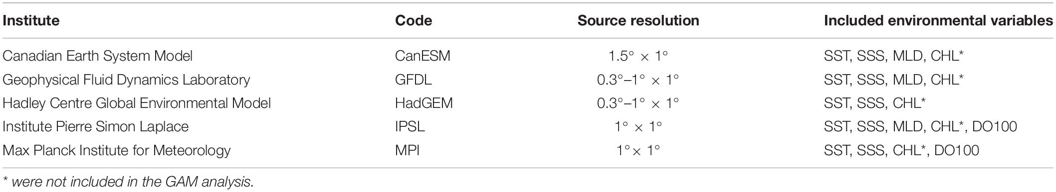
Table 1. List of IPCC atmosphere-ocean general circulation models where the future environmental variables, including the sea surface temperature (SST, °C), sea surface salinity (SSS, PSU), mixed layer depth (MLD, m), chlorophyll-a concentration (CHL, kg L–1), and dissolved oxygen concentration under 100 m depth (DO100, mmol L–1), were obtained to generate potential habitat maps of south Pacific albacore under ocean warming scenarios (RCP 4.5 and RCP 8.5).
A variety of approaches can be used to model the relationship between fish relative abundance and environmental variables for the species distribution models (SDMs) (e.g., MaxEnt, random forests, boosted regression trees, etc.) (Pickens et al., 2021). Because the focus of this paper for the ensemble analysis is to reduce the uncertainty in predictions of ocean conditions from AOGCMs rather than the uncertainty in model structure among various SDMs, therefore we only considered the most common method for predicting the relative abundance of tuna species, such as generalized linear modeling approach (Arrizabalaga et al., 2015; Lan et al., 2018; Erauskin-Extramiana et al., 2019). SDM of the south Pacific albacore was constructed by modeling fishery-dependent CPUEs in relation to the considered historical environmental variables using the generalized additive models (GAMs) (Hastie and Tibshirani, 1990; Wood, 2012, 2017). GAMs were selected rather than the GLMs (generalized linear models) because they can deal with multiple non-linear relationships between the covariates and the response variable in a semi-parametric manner (Hastie and Tibshirani, 1990). Apart from the continuous environmental variables, the year, quarter, flag were modeled as the categorical variables for the availability and/or catchability (Arrizabalaga et al., 2015). The raw CPUE data from the tuna longline fisheries includes many zeros. In this context, it was appropriate to fit the delta approach which models the probability of encounter of a fish population and the non-zero CPUE when fish are encountered (Pennington, 1983, 1996; Lo et al., 1992). Due to the low percentage of zero catches (<10%) of the quarterly 5° × 5° aggregated dataset that implying zero inflation was not an issue (Ichinokawa and Brodziak, 2010), we only fit the catch rate model using the log-transformed CPUEs of albacore, with a small constant (10% of the grand mean) added to avoid log-transformation problems (Campbell et al., 1996; Howell and Kobayashi, 2006; Mugo et al., 2010). GAMs were built using the gam function of the “mgcv” package in R-language (Wood, 2012). First, we constructed a full model by including all independent variables, it can be written as:
where μ is the intercept value; Year, Quarter, Flag are the fixed effect for year, quarter, and catchability of longline-fleet flag, respectively, and s(x) is a smoothing function for the independent covariates. To avoid overfitting, degrees of smoothness (“k” values) were set to less than or equal to 8 (Erauskin-Extramiana et al., 2019).
Five candidate models were selected by the dredge function of the “MuMIn” R-package (Barton, 2016). This function compares all possible model structures with different combinations of all independent variables from the full model, and ranks those models according to their Akaike information criterion (AIC) value and the goodness-of-fit measure (percent of deviance explained) (Bruge et al., 2016; Erauskin-Extramiana et al., 2019). Multicollinearity was tested by using the ggpairs function of the “GGally” R-package if any highly correlated environmental variables should be removed (Arrizabalaga et al., 2015). A pairwise correlation that exceeds a threshold of 0.5–0.7 is defined as the presence of high collinearity (Dormann et al., 2013). The relative importance of predictor variables was evaluated by the percentage relative changes in the explained deviance and the AIC value of dropping each main effects factor from the full GAM (Kwon et al., 2018). Model performance of the top five candidate models was validated using k-fold cross-validation method. We used k = 5, data were randomly split into five subsets, using 80% of data to validate the remaining 20% (Erauskin-Extramiana et al., 2019; Georgian et al., 2019). For each model, the average R2 value derived from CPUE observations and GAM predictions of training data and validation data, respectively, was calculated as a measure for goodness-of-fit. We defined the model of average R2 > 0.6 as a good prediction performance. A large difference between the training and testing R2 would indicate overfitting (Villarino et al., 2015; Erauskin-Extramiana et al., 2019). The model with the lowest AIC and highest average R2 value was selected as the best model for the further analyses (Brewer et al., 2016).
Historical environmental data projected by the AOGCMs were used as inputs in the GAM to estimate the albacore distribution in 1997–2016. The predicted relative abundance values were then compared with the observed CPUE from the longline fisheries in 1997–2016 to evaluate the model performance for forecasting potential habitat. For estimating the future impacts of climate change on albacore distribution, the ensemble GAM projections (see Section “Ensemble Forecasting”) given the environmental conditions in the current (2020), mid (2050) and late (2080) periods of the twenty-first century derived from the five AOGCMs were compared to the projections of recent 5 years of 2012–2016 under two emission scenarios (RCP 4.5 and RCP 8.5). In the future habitat distribution projection (2020–2080) of each AOGCM, model projections were performed with the fixed factor “Year” kept at the mid-year between 1997 and 2016. Flag factor was set to a longline fleet (e.g., TW) that simply represents a scaling parameter for the catchability. For some AOGCMs (IPSL and HadGEM) that certain environmental variables were unavailable (MLD and DO100), the quarterly average value derived from other GCMs was used as a substitute.
This study used ensemble analysis to deal with the uncertainty between climate models, it has been proved to outperform a single model in past studies (Diniz-Filho et al., 2009; Crimmins et al., 2013). We used two ensemble methods to measure the distribution of the south Pacific albacore. First, the consensus forecasting (Araújo et al., 2005; Araújo and New, 2007) was made by calculating the central tendency (e.g., the mean or median) of the GAM predictions based on the environmental data projected by five AOGCMs under the RCP 4.5 and 8.5 scenarios, therefore reduce inter-model variances propagated from the AOGCMs. The median prediction is deemed less sensitive to outliers than the mean; therefore, in the present study, consensus forecasting was employed to GAMs predictions using the median value (Alabia et al., 2016). Furthermore, the spatial distributions of the anomaly of relative abundance of south Pacific albacore were calculated by subtracting the predictions from the median ensemble GAM projections by the current (2020), mid (2050), and late (2080) periods of the twenty-first century from the recent average of 2012–2016. The second ensemble approach used in this study was probabilistic forecasting. This involved computing the likelihood of the presence of preferred albacore habitats from each AOGCM and expressing this in the form of a probability map. The set of grid cells that may be considered preferred habitats were defined as those for which predicted relative abundance from the GAM is in the top 15% (Su et al., 2013). Thus, the probability of preferred habitats at each 1° × 1° cell was based on the percentage of five AOGCMs for which the predicted relative abundance at that location is considered preferred, called “agreement map” (Porfirio et al., 2014).
The potential relative abundance change averaged per grid cell for the south Pacific albacore under future climate change was estimated within the exclusive economic zones (EEZs) for the countries and territories in our study area. EEZ data (downloaded from http://www.marineregions.org) delimit the 200 nautical miles boundary from each coast (Flanders Marine Institute, 2018). This study only analyzed those countries or territories with more than 30% of the grid cells of fishery data inside the EEZ to ensure it was representative of relative abundance (Erauskin-Extramiana et al., 2019). For each RCP scenario, the change in relative abundance was calculated by subtracting the predicted relative abundance of median ensemble during the main fishing season within each EEZ in 2020, 2050, and 2080 from that in the recent 5 years of 2012-2016.
Scatterplots between environmental variables suggested low collinearity that the absolute values of correlation coefficients are less than 0.5 (Supplementary Figure 1). Results for each of the top five candidate models (model, predictor variables, effective degrees of freedom, AIC, P-value, and deviance explained) selected by dredge function were shown in Table 2. In all the models, the smooth terms were highly significant (P < 0.001). Overall, the full GAM had the lowest AIC value and the highest deviance explained (62.1%). Variable rankings based on the percentage relative changes in the explained deviance for the three most influential explanatory variables were: (1) DO100 (22.3%); (2) Flag (21.5%); and (3) SST (6.5%) (Supplementary Table 3). Cross-validation testing suggested that the full GAM had slightly better performance, with the highest R2 values for the training (0.62) and validation (0.61) datasets, compared to other candidate models (ranged 0.59–0.61 for both training and validation). A negligible difference in the R2 values indicated the absence of overfitting. Furthermore, the residuals of the full GAM conform well to the assumption of lognormality based on the distribution of residuals and quantile-quantile (QQ) plots (Supplementary Figure 2). Therefore, the full GAM was selected as the best model for the future habitat distribution prediction.
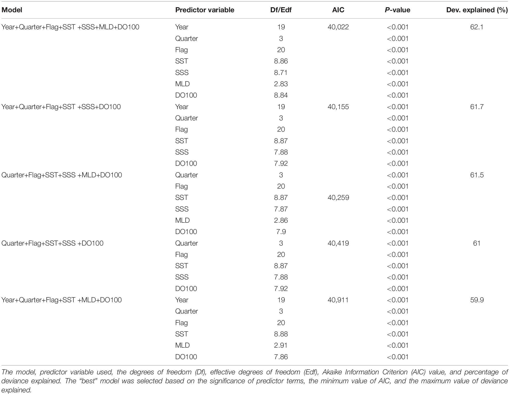
Table 2. Top five candidate models selected by the dredge function of the “MuMIn” R-package.
The response curves for environmental variables derived from the full GAM were interpreted in terms of habitat suitability of the south Pacific albacore. The fitted smooth curves show the preferred SST range of 13–22°C with a peak at around 15°C and SSS ranges of 34–35 PSU and > 36 PSU. Preferred MLD was between 20 and 60 m and the DO100 between 0.2 and 0.25 mmol L–1 (Figure 1). Approximate confidence interval envelopes were also plotted for each function. Lower precision was observed in the estimations for lower values of SST (<15°C), SSS (<34 PSU), DO100 (<0.1 mmol L–1) and higher values of MLD (>100 m) and DO100 (>0.25 mmol L–1) because of fewer data. The estimates of the year, quarter, and flag factors from the GAM were shown in Supplementary Figure 3. The year factor showed a significant decline during 1997–2003 and increase during 2004–2010. There is a significant seasonal variation in the quarter factor with the higher estimates in quarters 2 and 3. The flag factor showed higher estimates for CK, NC, US, and WS, but lower estimates for FM, AU, JP, KR, and NZ.
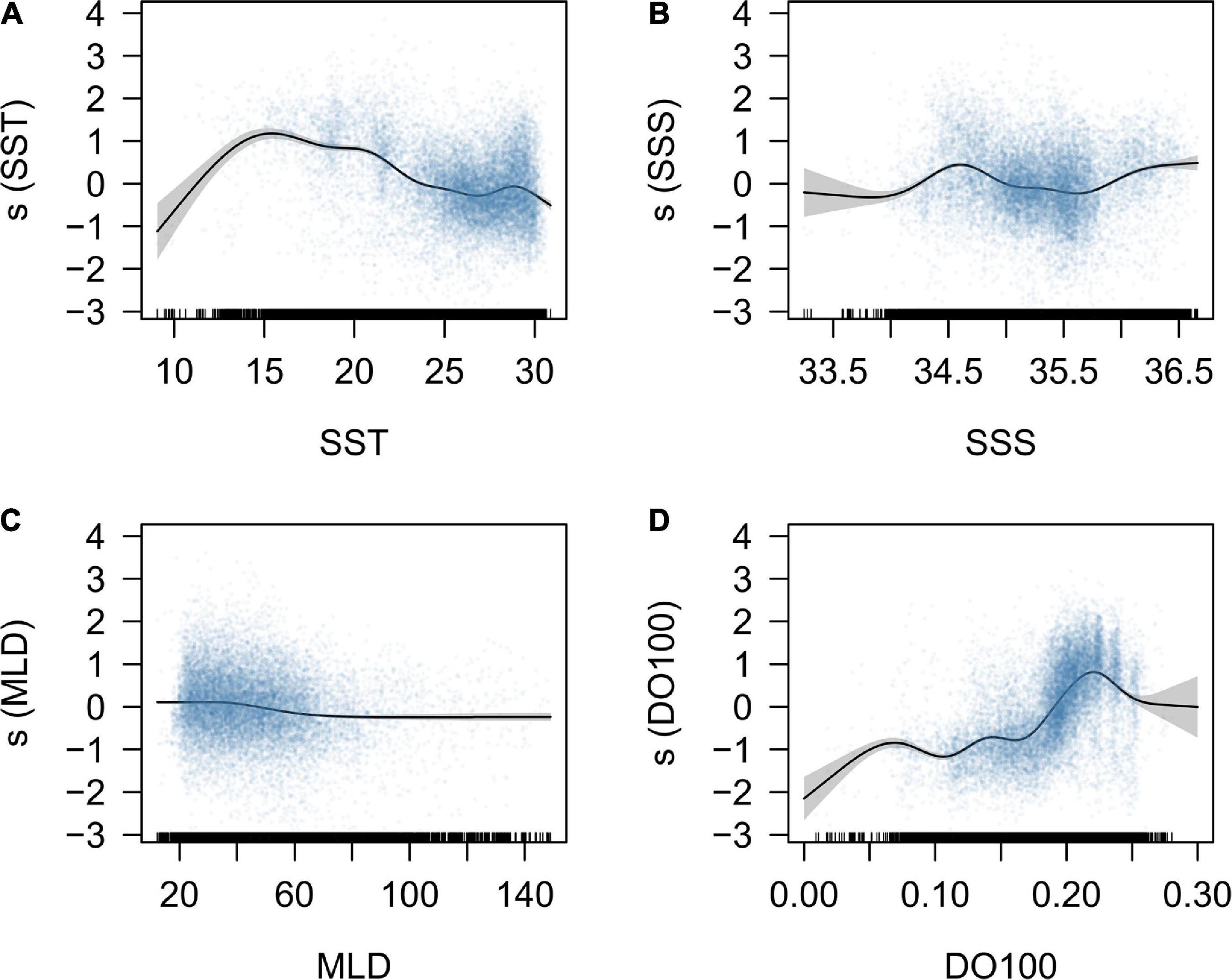
Figure 1. Response curves for the environmental variables, including the (A) sea surface temperature (SST, °C); (B) sea surface salinity (SSS, PSU); (C) mixed layer depth (MLD, m), and (D) dissolved oxygen concentration under 100 m depth (DO100, mmol L–1), derived from the GAM model. The blue points represent the partial residuals of observed CPUE data, and the gray polygons represent the 95% confidence interval. The hatch marks at the bottom are a descriptor of the frequency of data points.
The quarterly average distribution of albacore during 1997–2016 was shown in Figure 2. Model prediction has mimicked an apparent north-south seasonal variation of albacore distribution. The predicted spatial distributions in quarters 2–4 generally match well with the CPUE of longline vessels, in which the Pearson correlation coefficient (r) ranged from 0.62 to 0.71. However, the prediction fitted relatively poorly in the first quarter for the fishery data located north of 35°S (r = 0.6). In addition, annual aggregated CPUE values superimposed on the projected distributions had the r values ranged from 0.41 to 0.68, which indicated that the ensemble approach could generally yield reliable predictions overtime except for 2002.
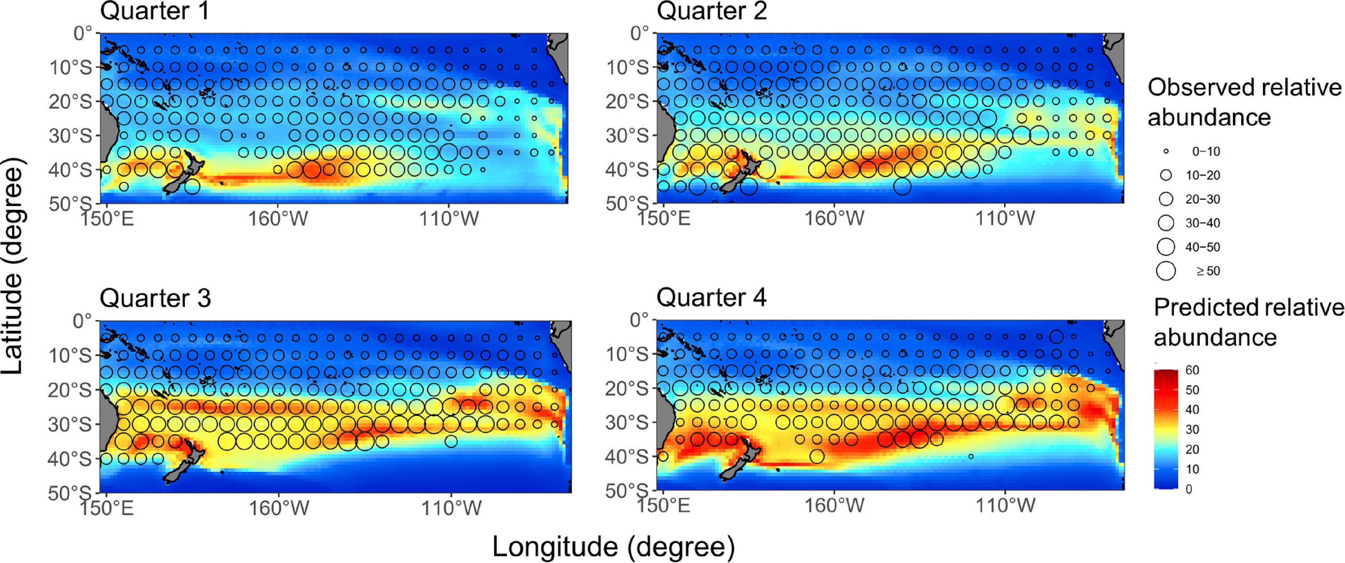
Figure 2. Quarterly average catch-per-unit-effort (CPUE) (number/1,000 hooks) distributions (open circles) for the south Pacific albacore overlaid on the median-ensemble relative abundance map (color contours) based on the GAM which was developed with data from 1997 to 2016.
Annual time-series of the areal-averaged of the environmental variables from 2020 to 2080 projected by the five AOGCMs were shown in Supplementary Figure 4. The predicted levels of environmental changes across the five AOGCMs exhibited differences in magnitude, for example, the lowest SST predictions by the IPSL and the highest by the HadGEM. Under the RCP 4.5, the median value was expected to increase from 20.8 to 21.1°C for SST, decrease from 81.3 to 73.9 m for MLD, and decrease from 0.22 to 0.218 mmol L–1 for DO100, respectively, during 2020-2080, while no trend was found in the SSS. Under the RCP 8.5, the more pronounced changes in SST with 2°C warming and in MLD with 12 m shallowed were observed during 2020–2080.
The future ensemble projections of albacore distributions in the main fishing season [i.e., quarter 3, which represents the highest (36%) historical harvest] derived from the five AOGCMs for the current (2020), mid (2050), and late (2080) periods of the twenty-first century by each RCP scenario were illustrated in Figure 3. The northern boundary of albacore preferred habitat (defined as CPUE > 25 number/1,000 hooks) in the western Pacific was projected to shift southward from 20°S in 2020 to 22°S in 2050 and 25°S in 2080 for the RCP 4.5. A similar pattern of southward shifting was observed for the RCP 8.5, with a wider spatial extent compared to the RCP 4.5. More specifically, the northern boundary has shown a similar degree of shifting as RCP 4.5, while the southern boundary in the Tasman Sea has shifted from 40°S in 2020 to 43°S in 2050 and 45°S in 2080.
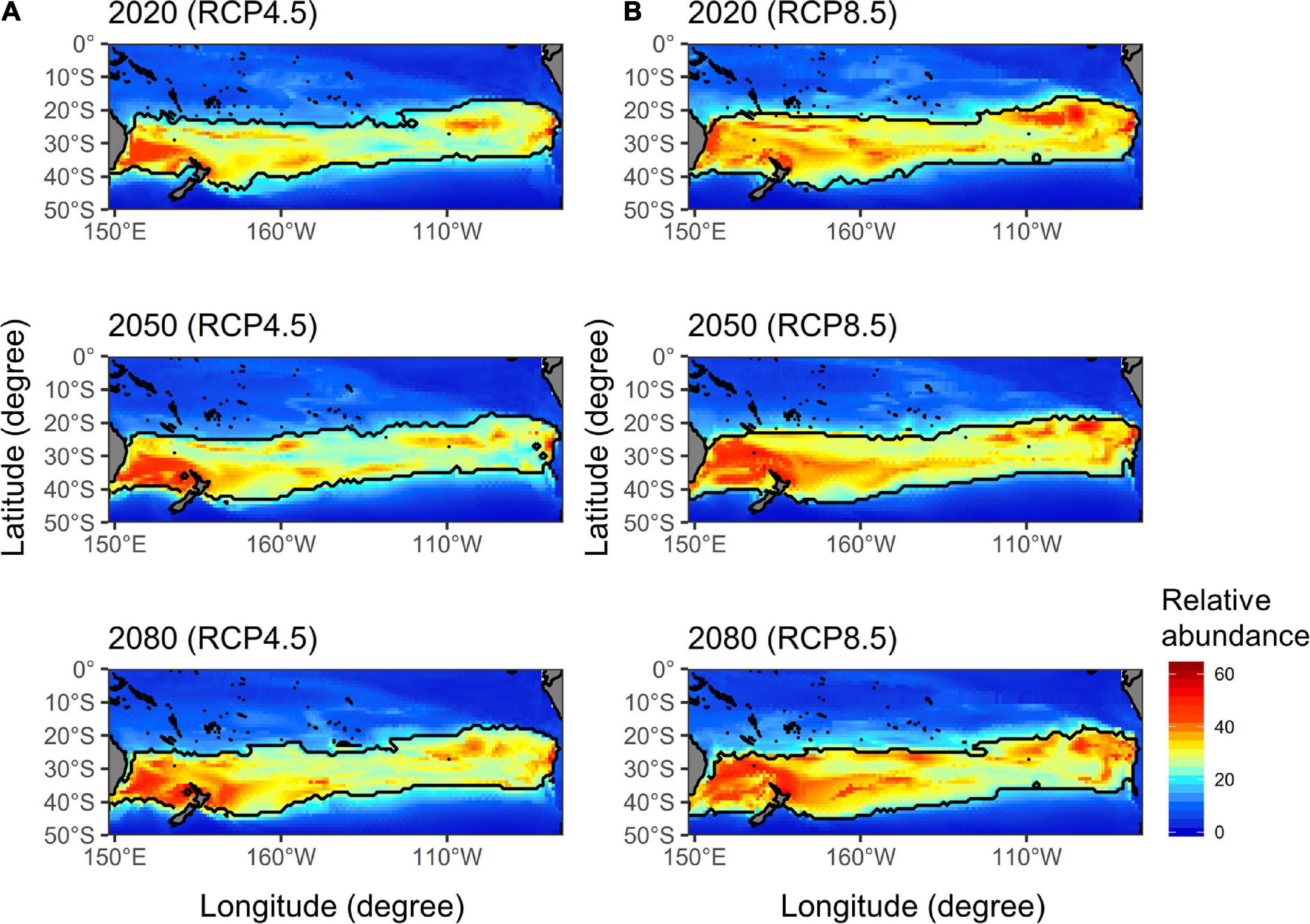
Figure 3. The future ensemble projections of south Pacific albacore relative abundance (number/1,000 hooks) distributions in quarter 3 estimated from the five atmosphere-ocean general circulation models (AOGCMs) for the current (2020), mid (2050), and late (2080) periods of the twenty-first century under the (A) RCP 4.5 and (B) RCP 8.5 (right panel) scenarios. The solid black lines denote the preferred habitat boundaries defined by relative abundance > 25 number/1,000 hooks.
The spatial distributions of the anomaly of relative abundance in quarter 3 by 2020, 2050, and 2080 under two RCP scenarios were shown in Figure 4. The potential albacore habitats increased in the latitudes of 30–40°S but decreased in 20–30°S of the western Pacific in 2020, 2050, and 2080 for the RCP 4.5, that the pattern of the gains and losses of potential habitat has become more apparent overtime. A similar pattern was observed for the RCP 8.5, however, the potential albacore habitats increased in the higher latitudes south of 40 °S in 2080 in the western Pacific, especially in the Tasman Sea, and in the eastern Pacific (east of 110 °W) during 2020–2080 compared to the RCP 4.5.
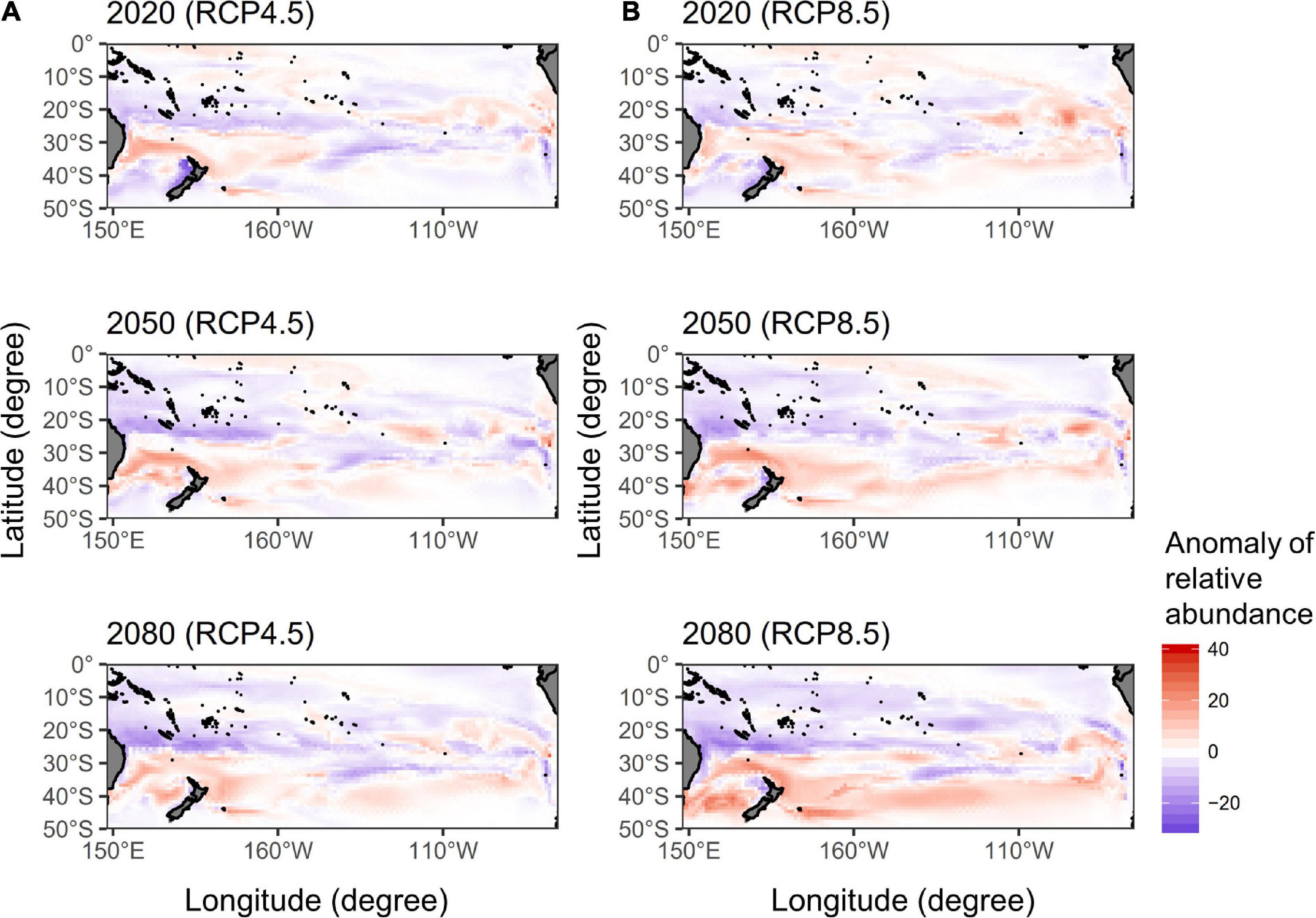
Figure 4. The spatial distributions of the anomaly of relative abundance for south Pacific albacore in quarter 3 calculated by subtracting the predictions of the median ensemble GAM projections in 2020, 2050, and 2080 from the recent average of 2012–2016 under the (A) RCP 4.5 and (B) RCP 8.5 scenarios.
Ensemble agreement maps for future albacore distribution in quarter 3 over five AOGCMs under two RCP scenarios were shown in Figure 5. For the RCP 4.5, the core habitats in western Pacific (red areas in Figure 5A) have shifted southward slightly during 2020–2080. The habitat ranges (blue areas) also shifted southward with an increase of 15% by 2050 and 16% by 2080 in the area south of 30°S relative to 2020, respectively. A similar southward displacement was also observed under the RCP 8.5 (Figure 5B), the latitudinal boundaries of core habitats showed an obvious southward shift in the Tasman Sea from 25 to 32°S in 2020 to 27–36°S in 2050 and to 32–39°S in 2080, respectively, and the habitat ranges in the area south of 30 °S increased 15% in 2050 and 21% in 2080.
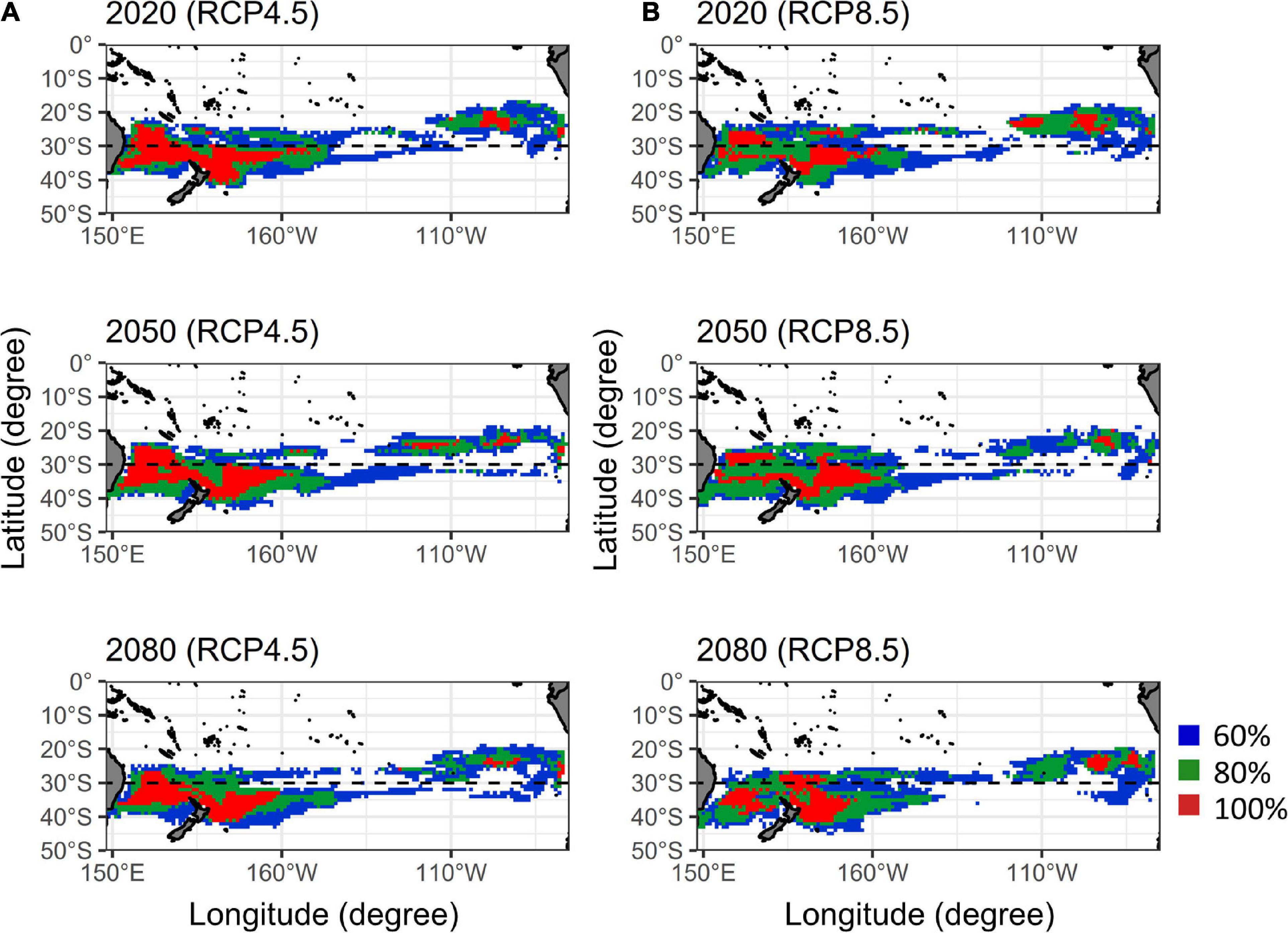
Figure 5. Ensemble agreement maps of the south Pacific albacore habitat predictions by five atmosphere-ocean general circulation models (AOGCMs) for the current (2020), mid (2050), and late (2080) periods of the twenty-first century under the (A) RCP 4.5 and (B) RCP 8.5 (right panel) scenarios. Colors denote the probabilities of habitat map based on the levels of agreement among five AOGCMs.
The results of the projected changes in albacore relative abundance during the main fishing season within the EEZs in 2020, 2050, and 2080 relative to 2012–2016 under the RCP 4.5 and 8.5 scenarios were shown in Figure 6. Under the RCP 4.5, albacore relative abundance is projected to decrease in most EEZs overtime (by about 25% in 2080), but was projected to slightly increase in 2020 and then decreased after 2050 for the EEZs of Kiribati (KI), Tuvalu (TV), and Tokelau (TK) (Figure 6A). The EEZ of New Caledonia (NC) has the greatest projected depletion in relative abundance by 2080 (43%). The relative abundance is projected to increase by 13 and 21% by 2080 in the EEZs of New Zealand (NZ) and Norfolk Island (NK), respectively. Similar patterns of relative abundance decline in most EEZs overtime were found for the RCP 8.5 (Figure 6B). A more significant negative and positive impact on the change of albacore relative abundance in 2080 was found for the EEZs of NC and both NZ and NK, respectively. The decline of relative abundance in 2080 for the EEZ of Australia (AUS) was slightly improved in RCP 8.5 (–2%) compared to RCP 4.5 (–11%).
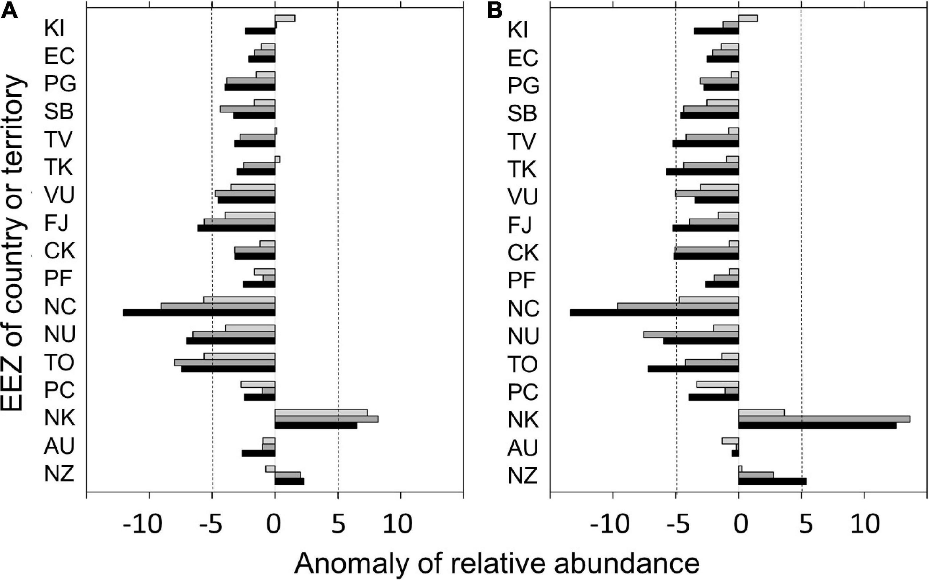
Figure 6. Changes in albacore relative abundance (number/1,000 hooks) within the exclusive economic zones (EEZs) of the countries or territories in the south Pacific Ocean for the current (2020), mid (2050), and late (2080) periods of the twenty-first century relative to 2012–2016 under the (A) RCP 4.5 and (B) RCP 8.5 scenarios. Only those countries or territories that had more than 30% of fishery data inside their EEZs were analyzed in this study. Countries or territories were ordered per mean latitude of the EEZ. The vertical dashed lines denote the reference line of ± 5 in anomaly of relative abundance. Country codes not shown in Supplementary Table 1 were illustrated below. EC, Galapagos Islands; TK, Tokelau; NU, Niue; PC, Pitcairn; NK, Norfolk Island.
In this study, we developed an ensemble forecast framework to evaluate the projected future potential distribution of south Pacific albacore under the scenarios of intermediate and high degrees of ocean warming (RCP 4.5 and RCP 8.5). The northern boundary of albacore preferred habitat is expected to shift southward by about 5° latitude and the relative abundance is expected to gradually increase south of 30°S from 2020 to 2080 for both RCP scenarios, especially with a higher degree of change for the RCP 8.5. This study highlights that investigating the future spatio-temporal patterns of the potential albacore habitats could lend significant implications on the availability of tuna resources to the fishery and subsequent evaluation of tuna fishery management options under climate change.
The results of this study may be considered as reliable predictions of the south Pacific albacore because the data used has contained a substantial amount (>90%) of the albacore catch and included all fleets covered a wide geographical range of the convention areas of the WCPFC and IATTC. Erauskin-Extramiana et al. (2019) only used the Japanese longline fishery data, constrained in the areas of 20°S northward and the waters off the eastern coast of Australia, which may not be informative to characterize the habitat preferences of albacore. Although the raw CPUE variability among various flags has been addressed in the GAM, the results with catchability adjustment can be biased due to the time-variant changes in fishing processes (e.g., gear saturation, fishing power, and fishing behavior). For example, the targeting tactic by Taiwanese distant water longline fishery has changed over time from only targeting albacore to both tropical tuna (mainly bigeye and yellowfin) and albacore (Chang et al., 2011). We recommend that the future albacore distribution model should further consider the possible changes in catchability to adjust the potential confounding effects on the estimation of relative abundance based on the detailed set-by-set longline data (including a variety of operational variables).
The south Pacific longline fisheries tend to exploit the larger size of albacore (>80 cm fork length) while the juvenile albacore is mainly targeted by the troll fishery near the coastal area of New Zealand (Hare et al., 2020; Jordán et al., 2021; Vidal et al., 2021). The projected results of this study may be considered as a proxy for the young adult and adult population. This highlights that using data from other types of fishing gear (i.e., troll fishery) may provide additional information to better understand the ontogenetic habitat preferences of the south Pacific albacore in future analysis.
The GAM used in this study was shown to robustly fit the data (deviance explained = 62%) because the residuals (in log-space) for the lognormal error distribution appear normal. Cross-validation testing also suggested that the GAM performed well without overfitting. However, quarter 1, not represents the main fishing season of albacore, had a relatively poor model performance compared to other quarters. The albacore may prefer a variety of habitat conditions in quarter 1 because some spawning adults in the second phase of spawning season are present in the tropical habitat of warmer temperature, but a large portion returns to their favorable feeding zones driven by the local cues in feeding habitat (Senina et al., 2019). A further extension of the GAM would be to estimate a seasonally variant habitat effect within the model, potentially improving the uncertainty of seasonal predictions. However, this was outside the scope of this study.
This study used a long-time series dataset (20 years of longline catch and effort data) with a wide range of observations for quantifying the relationships between the environmental variables and albacore catch rate, which improves the reliability of albacore response curve. Although all the environmental variables included in this study showed statistically significant impacts on albacore’s catch rate, the spatial distribution of albacore may be influenced by other factors in addition to the environmental variables used in the GAM. A range of observed or satellite-based oceanographic and biological variables has also been used to describe albacore-environment associations, including meridional and zonal geostrophic currents, sea surface height, thermal fronts, eddies, meso-zooplankton biomass over 0–100 m (Zainuddin et al., 2006; Lan et al., 2012; Xu et al., 2013; Arrizabalaga et al., 2015). However, one of the major issues to explore a broad range of oceanographic and biological variables for evaluating the future distribution shift is the availability of those variables from the future climate models. Furthermore, with a highly uncertain future environment, the predictions from AOGCMs could change in large amounts among each other compared to the historical predictions (e.g., CHL in this study). The above issues prevented further improvement for this study.
This study indicated that DO100 is the predominant environmental predictor of the distribution of south Pacific albacore because it contributed a substantial amount of explanatory power (22%) to the GAM. The albacore habitat was expected to decrease in the north of 15°S under the influence of a decrease in DO100 projected by the AOGCMs. The strong association between DO concentration and albacore distribution was confirmed by Lehodey et al. (2015) and Senina et al. (2018) through the sensitivity analysis in SEAPODYM that the future distribution and abundance of albacore tuna is likely to significantly decrease and remain stable in the South Pacific Ocean with and without a projected decrease in DO, respectively. The empirical study also supports the sensitivity of DO that albacore is not tolerant to low DO concentration compared to other tunas (Brill, 1994). On the other hand, studies indicated that albacore is highly sensitive to the temperature changes in both their spawning and feeding environments (Williams et al., 2015; Reglero et al., 2017), which is in agreement with the GAM analysis of this study that SST is considered as the second most important environmental factor (6%). Furthermore, the pronounced spatial changes in potential future albacore habitats could be also explained by the substantial changes in projected SST under ocean warming scenarios. This emphasizes that accuracy and precision in ensemble forecasts of albacore tuna distribution are fundamentally linked to the performance of the AOGCMs in being able to realistically describe future changes in DO and SST.
The southward distribution shift and changes in habitat suitability of south Pacific albacore identified in this study are consistent with the previous studies (Lehodey et al., 2015; Erauskin-Extramiana et al., 2019). However, the expected southward shift found by the above studies did not agree well with the study by Senina et al. (2018). This is due to the temperature spawning function implemented in SEAPODYM by Senina et al. (2018) tends to estimate a warmer favorable spawning habitat, resulted in future projected spawning ground similar to the present day. This indicated the importance of understanding the biological mechanism associated with shifts in albacore spawning ground under ocean warming. In addition, the distribution of albacore could be strongly influenced by the changes in growth, reproduction, and survival rate, and therefore the relevant mechanisms should be investigated in further analysis.
The uncertainty among the projections from the five AOGCMs and the two ocean warming scenarios that represent the plausible atmospheric forcings and emission pathways was taken into account through the ensemble analysis in this study. In addition to the uncertainty of climate projections, it would be desirable to explore other species distribution modeling approaches (e.g., Random forest, Maximum entropy, and Boosted regression tree models) to reduce the risk that structural inadequacies, inappropriate parameter specifications, or bias in each approach may unduly influence the final outputs (Robert et al., 2016; Georgian et al., 2019). Although ensemble forecasting could emphasize the “signal” that one is interested in emerges from the “noise” associated with individual model errors and uncertainties, the overall ensemble accuracy remains dependent on individual predictions (Araújo and New, 2007). Therefore, better individual forecasts will provide better combined forecast. Despite these issues, the ensemble forecasting approach could substantially reduce the likelihood of making false management decisions based on predictions that are far from the truth.
In this study, the albacore abundance is projected to decrease in most EEZs by 2080 with the greatest depletion for New Caledonia, but is projected to increase for New Zealand and Norfolk Island. The projections by Senina et al. (2018) indicated that the largest biomass increases occurred in the EEZs of Palau, Papua New Guinea, Federated States of Micronesia and Nauru at the end of the century under the simulation scenario with projected changes in the DO concentration, but decreases in the EEZs of Fiji, New Caledonia, and Vanuatu. Erauskin-Extramiana et al. (2019) suggested that the south Pacific albacore abundance would decrease in Kiribati, Tuvalu, Tokelau, Cook Islands, and Australia, but an increase in New Zealand. The result of this study generally supports the published evidence of the expected changes of albacore abundance in EEZs of PICTs except for the Palau, Federated States of Micronesia, and Nauru. The reason why those EEZs was not identified is because the present study only analyzed the countries or territories with more than 30% of the grid cells of fishery data inside the EEZs. Although the present study showed a decrease of abundance for Australia compared to the identified increase by Erauskin-Extramiana et al. (2019), Australia was found to have the smallest decrease of abundance among all countries and territories that located in the study area under the RCP 8.5. Currently, the conservation management measure (CMM-2015-2) for south Pacific albacore by the WCPFC has forbidden any increase in fishing vessels south of 20°S above 2005 levels (WCPFC, 2015). Under the current fishing effort constraint by the CMM, the future harvest catch of south Pacific albacore is expected to decrease because the potential albacore habitats are likely to increase in the latitudes of 30–40°S but decreased in 20–30°S of the western Pacific. This suggests that the effectiveness of CMM to achieve the fishery management goals could be impacted by the future potential distribution shifting. We assert not only the need but also the feasibility of incorporating approaches to address such shifts directly in the analysis of stocks and the management (e.g., management strategies evaluation, Punt et al., 2016) based thereon, so that the stock can be managed in a proactive and precautionary manner.
The raw data supporting the conclusions of this article will be made available by the authors, without undue reservation.
Y-JC, JH, and P-KL contributed to the development of the concept, analysis of the data, and writing of this manuscript. K-WL and W-PT provided the fisheries data and future environmental data and contributed to writing those sections of the manuscript related to this. All authors read and agreed to the published version of the manuscript.
This study was financially supported by the Ministry of Science and Technology and the Fishery Agency of Council of Agriculture of Taiwan through the research grants MOST109-2611-M-002-013- and 110AS-6.1.1-FA-F1.
The authors declare that the research was conducted in the absence of any commercial or financial relationships that could be construed as a potential conflict of interest.
All claims expressed in this article are solely those of the authors and do not necessarily represent those of their affiliated organizations, or those of the publisher, the editors and the reviewers. Any product that may be evaluated in this article, or claim that may be made by its manufacturer, is not guaranteed or endorsed by the publisher.
We are grateful to the Overseas Fisheries Development Council (OFDC) of Taiwan for providing data from the Taiwanese longline fishery. We also thank the Western and Central Pacific Fisheries Commission and Inter-American Tropical Tuna Commission for providing public fishery data of South Pacific albacore. We thank Shui-Kai Chang and Chiee-Young Chen who have both contributed to discussions regarding the species distribution modeling approach and ensemble forecast.
The Supplementary Material for this article can be found online at: https://www.frontiersin.org/articles/10.3389/fmars.2021.731950/full#supplementary-material
Alabia, I. D., Saitoh, S. I., Igarashi, H., Ishikawa, Y., Usui, N., Kamachi, M., et al. (2016). Future projected impacts of ocean warming to potential squid habitat in western and central North Pacific. ICES J. Mar. Sci. 75, 1343–1356. doi: 10.1093/icesjms/fsv203
Araújo, M. B., and New, M. (2007). Ensemble forecasting of species distributions. Trends Ecol. Evol. 22, 42–47. doi: 10.1016/j.tree.2006.09.010
Araújo, M. B., Pearson, R. G., Thuiller, W., and Erhard, M. (2005). Validation of species–climate impact models under climate change. Glob. Change Biol. Bioener. 11, 1504–1513.
Arrizabalaga, H., Dufour, F., Kell, L., Merino, G., Ibaibarriaga, L., Chust, G., et al. (2015). Global habitat preferences of commercially valuable tuna. Deep Sea Res. Part II Top. 113, 102–112. doi: 10.1016/j.dsr2.2014.07.001
Barton, K. (2016). Package “MuMIn”: Multi-Model Inference. R package, Version 1.15. 6. Vienna: R Core Team.
Beaumont, L. J., Hughes, L., and Pitman, A. J. (2008). Why is the choice of future climate scenarios for species distribution modelling important? Ecol. Lett. 11, 1135–1146.
Bell, J. D., Reid, C., Batty, M. J., Lehodey, P., Rodwell, L., Hobday, A. J., et al. (2013). Effects of climate change on oceanic fisheries in the tropical Pacific: implications for economic development and food security. Clim. Change 119, 199–212. doi: 10.1007/s10584-012-0606-2
Brewer, M. J., Butler, A., and Cooksley, S. L. (2016). The relative performance of AIC, AICC and BIC in the presence of unobserved heterogeneity. Methods Ecol. Evol. 7, 679–692. doi: 10.1111/2041-210X.12541
Briand, K., Molony, B., and Lehodey, P. (2011). A study on the variability of albacore (Thunnus alalunga) longline catch rates in the southwest Pacific Ocean. Fish. Oceanogr. 20, 517–529. doi: 10.1111/j.1365-2419.2011.00599.x
Brill, R. W. (1994). A review of temperature and oxygen tolerance studies of tunas pertinent to fisheries oceanography, movement models and stock assessments. Fish. Oceanogr. 3, 204–216. doi: 10.1111/j.1365-2419.1994.tb00098.x
Brouwer, S., Pilling, G., and Williams, P. (2018). “Trends in the South Pacific Albacore Longline and Troll Fisheries,” in Working paper WCPFC-SC14-2018/SA-IP-08 (Rev. 2) presented to the Fourteenth Meeting of the Scientific Committee of the Western and Central Pacific Fisheries Commission, Majuro, Republic of the Marshall Islands, 6-14 August 2014, (Kolonia: Western and Central Pacific Fisheries Commission).
Bruge, A., Alvarez, P., Fontán, A., Cotano, U., and Chust, G. (2016). Thermal niche tracking and future distribution of Atlantic mackerel spawning in response to ocean warming. Front. Mar. Sci. 3:86. doi: 10.3389/fmars.2016.00086
Campbell, R. A., Tuck, G., Tsuji, S., and Nishida, T. (1996). “Indices of abundance for southern bluefin tuna from analysis of fine-scale catch and effort data,” in Working Paper SBFWS/96/16 Presented at the Second CCSBT Scientific Meeting, Hobart, Australia, (Hobart,TAS: CCSBT).
Chang, S. K., Hoyle, S., and Liu, H. I. (2011). Catch rate standardization for yellowfin tuna (Thunnus albacares) in Taiwan’s distant-water longline fishery in the Western and Central Pacific Ocean, with consideration of target change. Fish. Res. 107, 210–220. doi: 10.1016/j.fishres.2010.11.004
Childers, J., Snyder, S., and Kohin, S. (2011). Migration and behavior of juvenile North Pacific albacore (Thunnus alalunga). Fish. Oceanogr. 20, 157–173.
Crimmins, S. M., Dobrowski, S. Z., and Mynsberge, A. R. (2013). Evaluating ensemble forecasts of plant species distributions under climate change. Ecol. Modell. 266, 126–130. doi: 10.1016/j.ecolmodel.2013.07.006
Diniz-Filho, J. A. F., Mauricio Bini, L., Fernando Rangel, T., Loyola, R. D., Hof, C., Nogués-Bravo, D., et al. (2009). Partitioning and mapping uncertainties in ensembles of forecasts of species turnover under climate change. Ecography 32, 897–906. doi: 10.1111/j.1600-0587.2009.06196.x
Dormann, C. F., Elith, J., Bacher, S., Buchmann, C., Carl, G., Carré, G., et al. (2013). Collinearity: a review of methods to deal with it and a simulation study evaluating their performance. Ecography 36, 27–46. doi: 10.1111/j.1600-0587.2012.07348.x
Erauskin-Extramiana, M., Arrizabalaga, H., Hobday, A. J., Cabré, A., Ibaibarriaga, L., Arregui, I., et al. (2019). Large-scale distribution of tuna species in a warming ocean. Glob. Change Biol. 25, 2043–2060. doi: 10.1111/gcb.14630
FAO (2021). FishStatJ Manual. Version 4.01.5. Rome: Food And Agriculture Organization of the United Nations.
Flanders Marine Institute (2018). Maritime boundaries geodatabase Maritime boundaries and exclusive economic zones (200NM), version 10. Ostend: Flanders Marine Institute.
Ganachaud, A. S., Sen Gupta, A., Orr, J. C., Wijffels, S. E., Ridgway, K. R., Hemer, M. A., et al. (2011). “Observed and expected changes to the tropical Pacific Ocean,” in Vulnerability of tropical pacific fisheries and aquaculture to climate change, eds J. Bell, J. E. Johnson, and A. J. Hobday (Noumea: Secretariat of the Pacific Community), 115–202.
Georgian, S. E., Anderson, O. F., and Rowden, A. A. (2019). Ensemble habitat suitability modeling of vulnerable marine ecosystem indicator taxa to inform deep-sea fisheries management in the South Pacific Ocean. Fish. Res. 211, 256–274.
Gloria, M. B. A., Daeschel, M. A., Craven, C., and Hilderbrand, K. S. Jr. (1999). Histamine and other biogenic amines in albacore tuna. J. Aquat. Food Prod. Technol. 8, 55–69.
Hare, S., Williams, P., and Pilling, G. The Wcpfc Secretariat. (2020). “Trends in the South Pacific albacore longline and troll fisheries,” in Working Paper WCPFC-SC16-2020/SA-IP-11 (Rev. 01) presented to the Sixteenth Meeting of the Scientific Committee of the Western and Central Pacific Fisheries Commission, Electronic Meeting, 11-20 August 2020, (Kolonia: Western and Central Pacific Fisheries Commission).
Hastie, T. J., and Tibshirani, R. J. (1990). Generalized additive models, Vol. 43. Florida, FL: CRC press.
Hobday, A. J. (2010). Ensemble analysis of the future distribution of large pelagic fishes off Australia. Prog. Oceanogr. 86, 291–301. doi: 10.1016/j.pocean.2010.04.023
Howell, E. A., and Kobayashi, D. R. (2006). El Nino effects in the Palmyra Atoll region: oceanographic changes and bigeye tuna (Thunnus obesus) catch rate variability. Fish. Oceanogr. 15, 477–489. doi: 10.1111/j.1365-2419.2005.00397.x
Ichinokawa, M., and Brodziak, J. (2010). Using adaptive area stratification to standardize catch rates with application to North Pacific swordfish (Xiphias gladius). Fish. Res. 106, 249–260. doi: 10.1016/j.fishres.2010.08.001
Jordán, C. C., Hampton, J., Ducharme-Barth, N., Xu, H., Vidal, T., Williams, P., et al. (2021). “Stock assessment of South Pacific albacore tuna,” in Working Paper WCPFC-SC17-2021/SA-WP-02 (Rev. 02) presented to the Seventeenth Meeting of the Scientific Committee of the Western and Central Pacific Fisheries Commission. Online Meeting, 11-19 August 2021, (Kolonia: Western and Central Pacific Fisheries Commission).
Kwon, Y., Larsen, C. P., and Lee, M. (2018). Tree species richness predicted using a spatial environmental model including forest area and frost frequency, eastern USA. PLoS One 13:e0203881. doi: 10.1371/journal.pone.0203881
Lan, K. W., Kawamura, H., Lee, M. A., Lu, H. J., Shimada, T., Hosoda, K., et al. (2012). Relationship between albacore (Thunnus alalunga) fishing grounds in the Indian Ocean and the thermal environment revealed by cloud-free microwave sea surface temperature. Fish. Res. 113, 1–7. doi: 10.1016/j.fishres.2011.08.017
Lan, K. W., Lee, M. A., Chou, C. P., and Vayghan, A. H. (2018). Association between the interannual variation in the oceanic environment and catch rates of bigeye tuna (Thunnus obesus) in the Atlantic Ocean. Fish. Oceanogr. 27, 395–407.
Langley, A., and Hampton, J. (2005). “Stock assessment of albacore tuna in the south Pacific Ocean,” in Working Paper WCPFC-SC01-2005/SA-WP03 presented to the First Meeting of the Scientific Committee of the Western and Central Pacific Fisheries Commission. Noumea, New Caledonia, 8-15 August 2005, (Kolonia: Western and Central Pacific Fisheries Commission).
Lehodey, P., Senina, I., and Murtugudde, R. (2008). A spatial ecosystem and populations dynamics model (SEAPODYM)-Modeling of tuna and tuna-like populations. Prog. Oceanogr. 78, 304–318. doi: 10.1111/fog.12259
Lehodey, P., Senina, I., Nicol, S., and Hampton, J. (2015). Modelling the impact of climate change on South Pacific albacore tuna. Deep Sea Res. Part II Top. 113, 246–259. doi: 10.1016/j.dsr2.2014.10.028
Lo, N. C. H., Jacobson, L. D., and Squire, J. L. (1992). Indices of relative abundance from fish spotter data based on delta-lognornial models. Can. J. Fish. Aquatic Sci. 49, 2515–2526. doi: 10.1139/f92-278
Maunder, M. N., and Punt, A. E. (2004). Standardizing catch and effort data: a review of recent approaches. Fish. Res. 70, 141–159. doi: 10.1016/j.fishres.2004.08.002
Mugo, R., Saitoh, S. I., Nihira, A., and Kuroyama, T. (2010). Habitat characteristics of skipjack tuna (Katsuwonus pelamis) in the western North Pacific: a remote sensing perspective. Fish. Oceanogr. 19, 382–396. doi: 10.1111/j.1365-2419.2010.00552.x
Novianto, D., and Susilo, E. (2016). Role of sub surface temperature, salinity and chlorophyll to albacore tuna abundance in Indian Ocean. Indones. Fish. Res. 22, 17–26. doi: 10.15578/ifrj.22.1.2016.17-26
Pennington, M. (1983). Efficient estimators of abundance, for fish and plankton surveys. Biometrics 1983, 281–286. doi: 10.2307/2530830
Pennington, M. (1996). Estimating the mean and variance from highly skewed marinedata. Fish. Bull. U S. 94, 489–450.
Pickens, B. A., Carroll, R., Schirripa, M. J., Forrestal, F., Friedland, K. D., and Taylor, J. C. (2021). A systematic review of spatial habitat associations and modeling of marine fish distribution: A guide to predictors, methods, and knowledge gaps. PLoS One 16:e0251818. doi: 10.1371/journal.pone.0251818
Pilling, G. M., Berger, A. M., Reid, C., Harley, S. J., and Hampton, J. (2016). Candidate biological and economic target reference points for the South Pacific albacore longline fishery. Fish. Res. 174, 167–178. doi: 10.1016/j.fishres.2015.09.018
Porfirio, L. L., Harris, R. M., Lefroy, E. C., Hugh, S., Gould, S. F., Lee, G., et al. (2014). Improving the use of species distribution models in conservation planning and management under climate change. PLoS One 9:e113749. doi: 10.1371/journal.pone.0113749
Punt, A. E., Butterworth, D. S., de Moor, C. L., De Oliveira, J. A., and Haddon, M. (2016). Management strategy evaluation: best practices. Fish Fish. 17, 303–334. doi: 10.1111/faf.12104
Reglero, P., Santos, M., Balbín, R., Laíz-Carrión, R., Alvarez-Berastegui, D., Ciannelli, L., et al. (2017). Environmental and biological characteristics of Atlantic bluefin tuna and albacore spawning habitats based on their egg distributions. Deep Sea Res. Pt. I 140, 105–116. doi: 10.1016/j.dsr2.2017.03.013
Riahi, K., Rao, S., Krey, V., Cho, C., Chirkov, V., Fischer, G., et al. (2011). RCP 8.5 - A scenario of comparatively high greenhouse gas emissions. Clim. Change 109:33. doi: 10.1007/s10584-011-0149-y
Robert, K., Jones, D. O., Roberts, J. M., and Huvenne, V. A. (2016). Improving predictive mapping of deep-water habitats: Considering multiple model outputs and ensemble techniques. Deep Sea Res. Pt. I. 113, 80–89. doi: 10.1016/j.dsr.2016.04.008
Senina, I. N., Lehodey, P., Hampton, J., and Sibert, J. (2019). Quantitative modelling of the spatial dynamics of South Pacific and Atlantic albacore tuna populations. Deep Sea Res. Pt. I. 2019:104667. doi: 10.1016/j.dsr2.2019.104667
Senina, I., Lehodey, P., Calmettes, B., Dessert, M., Hampton, J., Smith, N., et al. (2018). “Impact of climate change on tropical Pacific tuna and their fisheries in Pacific Islands waters and high seas areas,” in Working paper WCPFC-SC14-2018/EB-WP-01 presented to the Fourteenth Meeting of the Scientific Committee of the Western and Central Pacific Fisheries Commission. Busan, Republic of Korea, 8-16 August 2018, (Kolonia: Western and Central Pacific Fisheries Commission).
Silva, C., Andrade, I., Yáñez, E., Hormazabal, S., and Barbieri, M. Á, et al. (2016). Predicting habitat suitability and geographic distribution of anchovy (Engraulis ringens) due to climate change in the coastal areas off Chile. Prog. Oceanogr. 146, 159–174. doi: 10.1016/j.pocean.2016.06.006
Su, N. J., Sun, C. L., Punt, A. E., Yeh, S. Z., DiNardo, G., et al. (2013). An ensemble analysis to predict future habitats of striped marlin (Kajikia audax) in the North Pacific Ocean. ICES J. Mar. Sci. 70, 1013–1022. doi: 10.1093/icesjms/fss191
Thomson, A. M., Calvin, K. V., Smith, S. J., Kyle, G. P., Volke, A., et al. (2011). RCP4.5: a pathway for stabilization of radiative forcing by 2100. Clim. Change 109:77.
Tremblay-Boyer, L., McKechnie, S., and Harley, S. J. (2015). “Standardized CPUE for south Pacific albacore tuna (Thunnus alalunga) from operational longline data,” in Working Paper WCPFC-SC11-2015/SA-IP03 presented to the Eleventh Meeting of the Scientific Committee of the Western and Central Pacific Fisheries Commission. Pohnpei, Federated States of Micronesia, 5-13 August 2015, (Kolonia: Western and Central Pacific Fisheries Commission).
van Vuuren, D. P., Edmonds, J., Kainuma, M., Riahi, K., Thomson, A., Hibbard, K., et al. (2011). The representative concentration pathways: an overview. Clim. Change 109:5. doi: 10.1007/s10584-011-0148-z
Vidal, T., Jordán, C., Peatman, T., Ducharme-Barth, N., Xu, H., and Williams (2021). “Background analysis and data inputs for the 2021 South Pacific albacore tuna stock assessment,” in Working paper WCPFC-SC17-SA-IP-03 presented to the Seventeenth Meeting of the Scientific Committee of the Western and Central Pacific Fisheries Commission. Online Meeting, 11-19 August 2021, (Kolonia: Western and Central Pacific Fisheries Commission).
Villarino, E., Chust, G., Licandro, P., Butenschön, M., Ibaibarriaga, L., Larrañaga, A., et al. (2015). Modelling the future biogeography of North Atlantic zooplankton communities in response to climate change. Mar. Ecol. Prog. Ser. 531, 121–142. doi: 10.3354/meps11299
WCPFC (2015). Summary Report of the twelfth Regular Session of the Commission for the Conservation and Management of Highly Migratory Fish Stocks in the Western and Central Pacific Ocean; Kuta, Bali, Indonesia, 3-8. December, 2015. Kolonia: Western and Central Pacific Fisheries Commission.
WCPFC (2018). Summary Report of the Scientific Committee Fourteenth Regular Session; Busan, Republic of Korea, 8-16. August, 2018. Kolonia: Western and Central Pacific Fisheries Commission.
Williams, A. J., Allain, V., Nicol, S. J., Evans, K. J., Hoyle, S. D., et al. (2015). Vertical behavior and diet of albacore tuna (Thunnus alalunga) vary with latitude in the South Pacific Ocean. Deep Sea Res. Pt. II. 113, 154–169. doi: 10.1016/j.dsr2.2014.03.010
Wood, S. (2012). mgcv: Mixed GAM Computation Vehicle with GCV/AIC/REML smoothness estimation. R package version 1.7-17. Vienna: R Core Team.
Xu, Y., Teo, S. L., and Holmes, J. (2013). “Environmental Influences on Albacore Tuna (Thunnus alalunga) Distribution in the Coastal and Open Oceans of the Northeast Pacific: Preliminary Results from Boosted Regression Trees Models,” in Working Paper ISC/13/ALBWG-01/01 presented to the Thirteenth Meeting of the International Scientific committee on Tuna and Tuna-like Species in the North Pacific Ocean. Shanghai, China, 19-26 March 2013, (Kolonia: Western and Central Pacific Fisheries Commission).
Keywords: south Pacific albacore, ensemble forecasting, climate change, species distribution model, longline fisheries
Citation: Chang Y-J, Hsu J, Lai P-K, Lan K-W and Tsai W-P (2021) Evaluation of the Impacts of Climate Change on Albacore Distribution in the South Pacific Ocean by Using Ensemble Forecast. Front. Mar. Sci. 8:731950. doi: 10.3389/fmars.2021.731950
Received: 28 June 2021; Accepted: 08 September 2021;
Published: 28 September 2021.
Edited by:
Irene D. Alabia, Hokkaido University, JapanReviewed by:
Jose Carlos Báez, Spanish Institute of Oceanography (IEO), SpainCopyright © 2021 Chang, Hsu, Lai, Lan and Tsai. This is an open-access article distributed under the terms of the Creative Commons Attribution License (CC BY). The use, distribution or reproduction in other forums is permitted, provided the original author(s) and the copyright owner(s) are credited and that the original publication in this journal is cited, in accordance with accepted academic practice. No use, distribution or reproduction is permitted which does not comply with these terms.
*Correspondence: Yi-Jay Chang, eWpjaGFuZ0BudHUuZWR1LnR3
Disclaimer: All claims expressed in this article are solely those of the authors and do not necessarily represent those of their affiliated organizations, or those of the publisher, the editors and the reviewers. Any product that may be evaluated in this article or claim that may be made by its manufacturer is not guaranteed or endorsed by the publisher.
Research integrity at Frontiers
Learn more about the work of our research integrity team to safeguard the quality of each article we publish.