Response of Abundance and Distribution of Humboldt Squid (Dosidicus gigas) to Short-Lived Eddies in the Eastern Equatorial Pacific Ocean From April to June 2017

In this study, the eddy characteristics on the fishing ground of the Humboldt squid (Dosidicus gigas) in the eastern equatorial Pacific Ocean were detected based on geometrical characteristics with the flow field during April–June 2017. The influence of the eddies on the biophysical environment, D. gigas abundance, and habitat distribution were explored. The habitat was identified by fishery data, sea surface temperature (SST), vertical water temperature, and chlorophyll-a (Chl-a). Results indicated that the eddy lifetime was relatively short, with only three eddies persisting for more than 2 weeks. The number of eddies in each month showed a similar variability trend with the monthly average catch per unit effort (CPUE) of D. gigas. Two eddies were taken with a lifetime of above 2 weeks, which revealed that the environmental conditions around the eddies significantly changed. When the eddy persisted for 8–10 days, SST and vertical temperature gradually decreased, but Chl-a significantly increased. The habitat quality of D. gigas gradually increased, and the gravity center of the fishing ground was consistent with eddy movement. The eddy-induced Ekman pumping led to the transportation of deep waters with rich nutrients into the euphotic layer, promoted the reproduction of bait organisms, and yielded favorable water temperature conditions for D. gigas. These environmental changes aided the formation of high-quality habitats, which increase D. gigas abundance and catch and drive the shift of the gravity centers of fishing grounds with the eddy. Our findings suggested that eddy activities have significant impacts on D. gigas abundance and habitat distribution.

Introduction

The Eastern Equatorial Pacific Ocean is one of the most important fishing grounds in the world. In this region, the oceanographic conditions, such as mesoscale eddy and west boundary coastal upwelling, have a great impact on the distribution pattern of productivity, affecting the coastal and pelagic fisheries (Fernández-Álamo and Färber-Lorda, 2006; Lavín et al., 2006; Willett et al., 2006). Paticurlarly, mesoscale eddies have great influences on marine material transportation and heat transfer (Dong et al., 2014; Zhang et al., 2014). The wind-driven boundary currents along the eastern coast of the Pacific, such as the Peru Current System and the California Current System, drive eddy formation with seasonal variability (Penven et al., 2005; Chaigneau et al., 2009), which gradually shift westward and transport coastal nutrients to offshore waters (Fernández-Álamo and Färber-Lorda, 2006; Lavín et al., 2006; Willett et al., 2006).

The eddy can produce both upwellings and downwellings and affects biophysical environments. It redistributes nutrients and plankton and improves the material utilization efficiency of the ocean (Willett et al., 2006; Zhang et al., 2014; McGillicuddy, 2016). Mesoscale eddies increase food availability and affect fish distribution. There is high plankton density around cyclonic and anticyclonic eddies, which attract large cetaceans (e.g., whales and sharks) to gather in the northern part of the Gulf of Mexico (Davis et al., 2002). In the Mozambique Strait, eddies attract more seabirds (e.g., albatross and petrels) to forage (Kai and Marsac, 2010; De Monte et al., 2012). The equatorial waters off the eastern Pacific Ocean have a complex tropical ocean current system (Figure 1). The latitudinal barotropic unstable shear from affluents is the main factor for eddy generation, which is called “Tropical instability vortices (TIVS)” (Kennan and Flament, 2000; Willett et al., 2006). These eddies change the temperature and salinity in the equator and form intensive temperature fronts in the northern waters of the equator. In the meantime, large amounts of fish were observed around the eddies (Flament et al., 1996; Kennan and Flament, 2000).

FIGURE 1

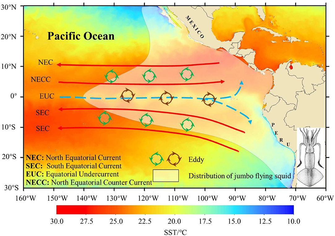
Figure 1. Geographical distribution of D. gigas with oceanic environmental conditions [major tropical Pacific currents, the eddy, and sea surface temperature (SST)] in the Eastern Pacific Ocean. The possible locations of eddies in the equatorial waters were based on the studies by Kennan and Flament (2000) and Zheng et al. (2016). The shaded color indicates the average monthly SST in May 2017. Different colors indicate the different directions of two kinds of eddies.

The Humboldt squid (Dosidicus gigas) is widely distributed in the eastern Pacific Ocean (Figure 1). This species is a crucial fishing target in the waters off Peru, Chile, Ecuador, and the Gulf of California due to its high economic value (Keyl et al., 2008; Csirke et al., 2015; Ibáñez et al., 2015). In 2001, China started to investigate and capture D. gigas stock off Peruvian waters, with a successful production of 17,000 t. The Chilean and equatorial fishing grounds were developed in 2004 and 2012, respectively (Chen and Zhao, 2005; Chen et al., 2012). Since 2017, more fishing vessels are used for fishing in the equator and accumulated fishing records. The life cycle of D. gigas is short, with a 1-year lifespan (Keyl et al., 2008). There are geographic differences in the mantle length of D. gigas. Under high-temperature and low-nutrient conditions (equatorial waters and the Costa Rica dome), the mantle length of the sexually mature D. gigas is shorter. Under low-temperature and high-nutrient conditions (the coast of Peru-Chile and the Gulf of California), the sexually mature mantle length is longer (Keyl et al., 2008; Csirke et al., 2015; Ibáñez et al., 2015).

Large-scale climatic events, such as El Niño and La Niña events and regional environmental changes, affect the growth, age structure, and population composition of D. gigas and change their habitat pattern and abundance (Keyl et al., 2008; Yu et al., 2017). In equatorial surface waters, South and North Equatorial Currents (surface) occur from westward to eastward and are located between the two Equatorial Currents under the influences of trade winds (Brown et al., 2007; Sen Gupta et al., 2012). In the subsurface layers of the equator, the Equatorial Undercurrent rises in the eastern waters. It carries rich nutrients, bringing the cold water from the subsurface layer to the surface layer. It can form a cold tongue, which has high productivity and extends westward (Brown et al., 2007). The equatorial waters have intensive eddy activities due to the complex tropical current system (Kennan and Flament, 2000; Brown et al., 2007). However, the effects of the eddy on D. gigas abundance and habitat distribution are rarely investigated.

In this study, the fishery data of Chinese squid-jigging fishing vessels were used from April to June 2017 in the equatorial waters, combined with environmental factors [vertical water temperature, currents, and chlorophyll-a (Chl-a)] to evaluate the influences of mesoscale eddies on the habitat distribution and D. gigas abundance in the equatorial waters. This study aimed to clarify the characteristics of eddies in the equatorial waters based on flow field data, select eddies with a relatively longer lifetime for evaluating their impacts on the biophysical environment of the equatorial waters, and examine the relationship between eddy activity and the abundance and habitat distribution D. gigas using the habitat suitability index (HSI) modeling approach.

Materials and Methods

Fisheries and Environmental Data

The fishery data in eastern equatorial Pacific waters were obtained from the fishing logbook of 48 Chinese squid-jigging fishing vessels from 17 distant-water fishery companies during April–June 2017. There were about 3,000 original fishing data records from April to June 2017, and the distribution of fishing position is shown in Figure 2. The data were obtained from the National Distant-water Fisheries Data Center of China (NDFDC), Shanghai Ocean University, Shanghai, China. The data information included the name of the company and fishing vessels, fishing location (latitude and longitude), fishing date (year, month, and day), catch (unit: ton), and fishing effort (fishing days). The spatial resolution of the fisheries data was 0.1°.

FIGURE 2

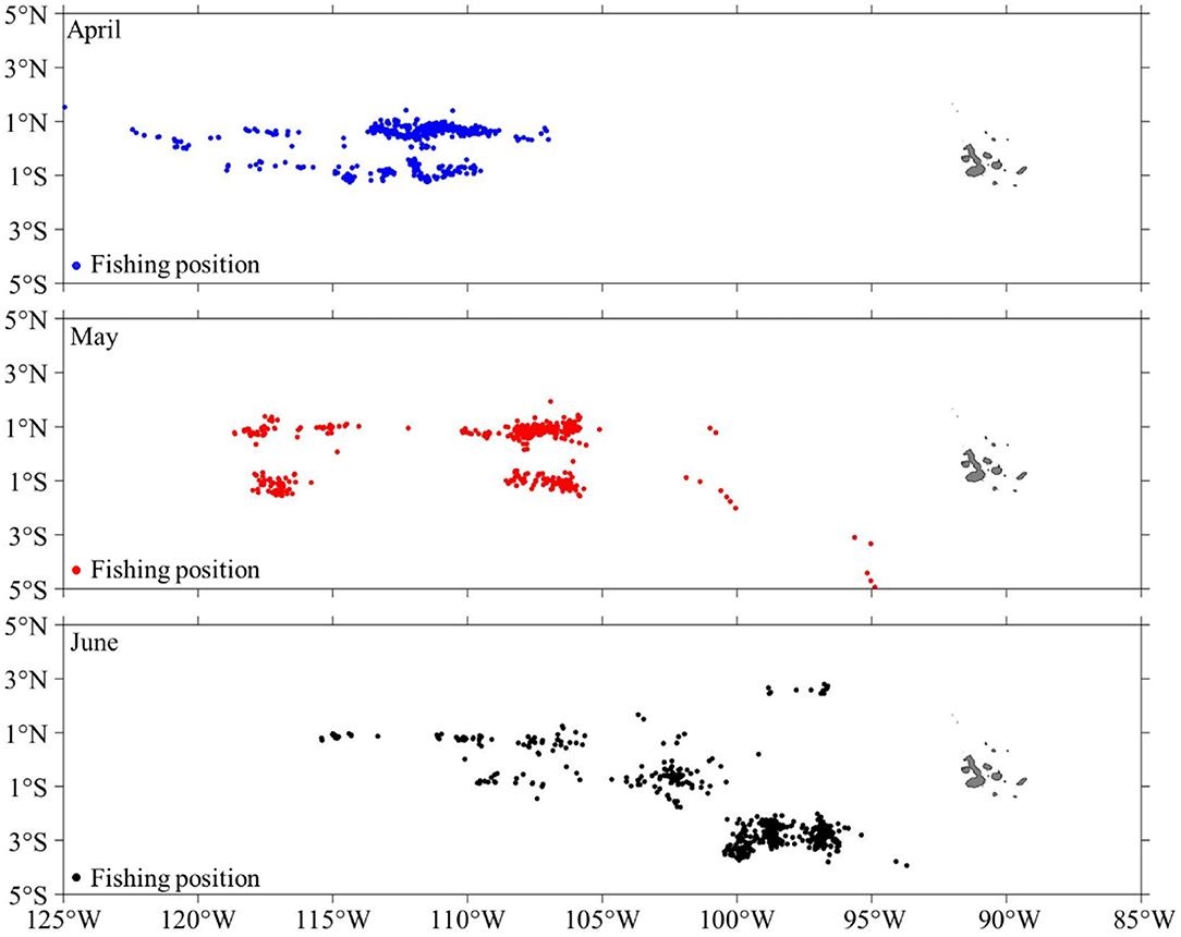
Figure 2. Monthly distributions of fishing positions for the Chinese squid-jigging vessels from April to June 2017 on the fishing ground of D. gigas in the equator.

The surface current field data were provided by the NetCDF Subset Service (NCSS) under Unidata. These data were downloaded from the Oceanwatch website (https://oceanwatch.pifsc.noaa.gov/thredds/ncss/grid/noaa_sla/dt/dataset.html). The dataset was not resampled or projected to retain the resolution and accuracy of the original datasets. The data content included gridded geostrophic field data (U: east component and V: north component) and sea level anomaly (SLA) data. The time resolution of the flow field data was 1 day with a 0.25° × 0.25° spatial resolution.

Sea surface temperature is an important environmental factor affecting D. gigas distribution (Chen and Zhao, 2005; Keyl et al., 2008). This species performs important diurnal vertical migrations, and the vertical structure of water temperature may have profound impacts on its distribution (Csirke et al., 2015; Ibáñez et al., 2015). The water temperature data were selected at seven different layers, namely, sea surface temperature (SST), Temp_30 m, Temp_50 m, Temp_75 m, Temp_100 m, Temp_120 m, and Temp_150 m. The vertical temperature data were obtained from the Asia Pacific Data Research Center (http://apdrc.soest.hawaii.edu/las_ofes/v6/constrain?var=95). The time resolution of all water temperature data was 3 days with a 0.1° × 0.1° spatial resolution.

Chlorophyll-a concentration was used to characterize the variability in nutrient levels around the eddy. The data were obtained from the Asia-Pacific Data Research Center (http://apdrc.soest.hawaii.edu/las/v6/constrain?var=13152). The time resolution of the Chl-a data was 1 day with a 4-km spatial resolution. All the environmental data covered the study area between 5°N−5°S and 125–85°W in the eastern Pacific Ocean from April to June 2017. The spatial resolution of all environmental data was retained by unifying the time resolution (3, 6, and 9 days) to examine the environmental changes under eddies. However, the spatial and temporal resolutions of all the environmental variables (except the current data) were resampled and consistent with the fishery data.

Methods

Eddy Detection and Tracking Algorithm

An eddy detection algorithm proposed by Nencioli et al. (2010) based on the flow field data by vector geometry was used in this study. The steps were as follows:

Step 1: Four constraints were used to identify the center of the eddy. (1) The current component U along the east–west direction of the center of the eddy had opposite signs on both sides, and its magnitude increased from the center. (2) The current component V along the north–south direction of the center of the eddy had opposite signs on both sides, and its magnitude increased from the center. (3) The minimum speed point in the selected area was found approximately at the center of the eddy. (4) The rotation direction of the velocity vector around the eddy center must be the same, indicating that the directions of two adjacent velocity vectors must be located in the same or two adjacent quadrants.

Step 2: The outermost closed streamline around the center was selected as the boundary of the eddy.

Step 3: When an eddy is detected at time t in the study area, and the same type of eddy (cyclonic or anticyclonic) can be detected at time t + 1 in this area. If an eddy cannot be located within the study area at t + 1, a second search will be taken at time t + 2 within the expended area of 1.5 times to avoid misjudging. If no eddy (same eddy) is detected at t + 2 within this area, this eddy is considered dissipated. Thus, the lifetime was defined according to the time of its existence.

Two parameters (a and b) should be defined in the process of eddy identification (Nencioli et al., 2010). The parameter “a” defines the number of grid points in the flow field data. The parameter “b” defines the dimension (in grid points) of the area used for describing the local minimum of velocity. The eddy recognition performance was considered the best when a = 2 and b = 3 (Lin et al., 2015). The flow field data with a 1-day resolution were used as input in the model. The eddies were identified in the equatorial waters off the eastern Pacific Ocean from April to June 2017, and eddy center position, lifetime, number, and radius were classified.

Assessment of the Impacts of Eddy on the Biophysical Environment

After eddy identification, two eddies with a relatively longer lifetime (more than 2 weeks, named eddy 1, and eddy 2) were selected. The lifetime of the eddy was divided into different temporal resolutions of 6 days. The time resolution of all the environmental data was preprocessed and consistent with the different periods of the selected eddies. To accurately clarify the changes in the environment, the original spatial resolution of each environmental datum was retained and extended to the two periods before the eddy was generated and after it disappeared. To explore the changes in the biological and physical environments in the different periods of the eddy, the distribution patterns of SST, the vertical temperature structure, and Chl-a concentration were examined. In addition, a quick sensitivity analysis on the different temporal resolutions of the eddy (3, 6, and 9 days) was performed to examine the impacts of the eddy on biophysical environments.

The Response of D. gigas Stock to Eddy

In this study, the fishery data [the catch, fishing effort, and catch per unit effort (CPUE)] were processed at a time resolution of 6 days and superimposed with the environmental layers (SST and Chl-a). The proportions of catch and fishing efforts of D. gigas in the whole study area were calculated, and the impacts of the environmental changes were evaluated on their distributions. In addition, the longitudinal gravity center of fishing effort (LONG) and CPUE in different periods were determined and compared with the eddy center. The LONG and CPUE were calculated with the following equations:

$LONG={\displaystyle \sum _{i=1}^k(C_i}\times X_i)/{\displaystyle \sum _{i=1}^k{C}_i}$

$\begin{array}{l}CPUE={\displaystyle \sum _{i=1}^k}{X}_i/{\displaystyle \sum _{i=1}^k}{E}_i\end{array}$

where X_idenotes the catch of the fishing position; C_idenotes the longitude of the fishing position; E_i denotes the effort of the fishing position; k is the number of fishing positions in different periods of the eddy.

Habitat Changes of D. gigas at Different Stages of the Eddy

An HSI model was established to examine the habitat changes of D. gigas around the eddy. The eddy 1 in this study lasted almost the entirety of May. Therefore, the habitat condition within eddy 1 was explored. Previous studies have shown that SST, Chl-a, and vertical water temperature have shown significant impacts on the habitat pattern of D. gigas in the equatorial waters (Yi et al., 2014; Fang et al., 2021). Therefore, four environmental factors, namely, SST, Chl-a, Temp_50 m, and Temp_100 m, were selected to develop the HSI model. All the environmental data were grouped by the 0.1° × 0.1° grid and were consistent with the spatio-temporal resolution of the fishery data. According to the frequency distribution method, the frequency distribution of fishing efforts at different intervals of environmental factors was calculated (Yu et al., 2021). The probability of occurrence of D. gigas at different ranges of each environmental variable was calculated and defined as a suitability index (SI). The SI curve of each environmental factor was constructed based on the environmental variable class interval and the corresponding SI values. For each environmental factor, the SI model was established as follows:

$\begin{array}{l}S{I}_{SST}=exp(c\times {(SST-d)}^2)\end{array}$

$\begin{array}{l}S{I}_{chl\text{\_}a}=exp(c\times {(Chl\text{\_}a-d)}^2)\end{array}$

$\begin{array}{l}S{I}_{Temp\text{\_}50m}=exp(c\times {(Temp\text{\_}50m-d)}^2)\end{array}$

$\begin{array}{l}S{I}_{Temp\text{\_}100m}=exp(c\times {(Temp\text{\_}100m-d)}^2)\end{array}$

where c and d are the estimated model parameters solved with a least-squares estimate to minimize the residuals between the observed and predicted SI values.

The empirical arithmetic mean method (AMM) determined the HSI for D. gigas in the eastern Pacific Ocean (Yu et al., 2016). Thus, the AMM-based HSI model was used to calculate the ultimate HSI. The equation of HSI was given as follows:

$\begin{array}{l}HSI=\frac{1}{4}(S{I}_{SST}+S{I}_{chl\_a}+S{I}_{Temp\_50m}+\text{}\\ \text{ }S{I}_{Temp\_100m})\end{array}$

where SI_SST, SI_{chl_a}, SI_{Temp_50m}, and SI_{Temp_100m} indicate the predicted SI value for each environmental variable. In this study, the areas with HSI ≤ 0.2, 0.2 < HSI < 0.6, and HSI ≥ 0.6 are defined as poor, common, and suitable habitats, respectively, for D. gigas (Yu et al., 2021).

Finally, the HSI model was tested and validated. When the proportion of the catch and fishing effort was the least in the poor habitat, it is the highest in the suitable habitat, and the prediction performance of the model was good. To estimate the changes in the habitat conditions of D. gigas, the average HSI and proportions of suitable and poor habitats in different periods of the eddy were calculated.

Results

Identification and Characteristic Analysis of the Eddies

In the study region, the model detected 195 eddies from April to June (Table 1), and the proportion of eddies with a lifetime of <7 days was 93%. There were only 11 and 3 eddies with a lifetime in the intervals of 8–14 days and higher than 2 weeks, respectively, accounting for 5 and 2% of the total number of eddies. The number of eddies in May was 71, which was the highest. There were two eddies with a lifetime of more than 14 days in May. The number of eddies in June was 56, which was the least, and there was no eddy with a lifetime of more than 2 weeks. In this study, two eddies (eddy 1 with a lifetime of 21 days and eddy 2 with a lifetime of 33 days) with a lifetime of more than 2 weeks in May were selected as case studies. The detail about the distribution of all eddies from April to June and the period division and tracks of two eddy cases are shown in Supplementary File 1.

TABLE 1

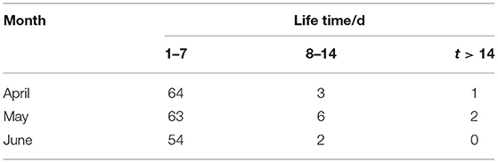
Table 1. The lifetime and number of eddies from April to June 2017 on the fishing ground of Dosidicus gigas in the eastern equatorial Pacific Ocean.

The Influences of Eddies on the Biophysical Environment

The SST and vertical temperature structures (equator: 0°) in the different periods of the two eddies are drawn in Figure 3. Before eddy 1 generation, the SST was relatively high, and the contour lines of the vertical temperature descended. The SST increased, and the contour lines of the vertical temperature were horizontal in period 1. The contour lines of the vertical temperature arose in period 2. The cold temperature areas gradually enlarged in periods 3 and 4. When the eddy disappeared, the cold temperature area shifted southward, and the rising contour lines of the vertical temperature shifted eastward. Similar to eddy 1, the SST of eddy 2 gradually decreased. With the eddy 2 shifting westward, the contour lines of the vertical temperature rose significantly from periods 5 to after eddy disappearance (AED). Comparing the temperature structure at AED and the last period (eddy 1: period 4; eddy 2: period 6) (Figures 3A,B), the eddy could drive the contour lines of vertical temperature rising and SST decreasing. With the sustained effects of the two eddies, SST decreased from 27°C (before the eddy generation, BEG) to approximately 25°C at the final period (Figures 3C,D). Two eddies could make the temperature decrease effectively.

FIGURE 3

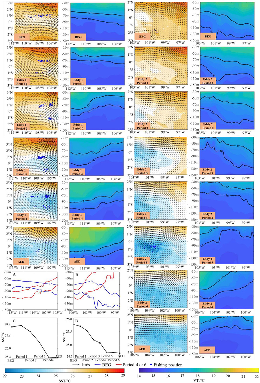
Figure 3. Spatial distribution of SST and vertical temperature structure (VT) with the effects of eddies 1 and 2. (A) (eddy 1) and (B) (eddy 2) show the isothermal line of the vertical temperature structure (16 and 17°C) during the period of the BEG (before the eddy generation, blue line) and period 4 of eddy 1 and period 6 of eddy 2 (red line). (C) (eddy 1) and (D) (eddy 2) show the variations of average SST in different periods.

As shown in Figure 4, the Chl-a concentration was low in the BEG of eddy 1 and then gradually increased from period 1 to AED. The area with high Chl-a concentration gradually shifted northeastward along the south side in period 1, and the east side of eddy 1 was the highest. However, in periods 3 and 4, the Chl-a concentration on the south side of the eddy gradually increased. The Chl-a concentration rose in the AED, and the high Chl-a concentration area gradually expanded to the north. For eddy 2, the Chl-a concentration decreased in period 2, and then gradually increased. The high Chl-a concentration area showed an upsweep from the middle and passed through the center in periods 4 and 5. However, the Chl-a concentration in the northern waters was significantly higher than other regions in period 6. The waters with high Chl-a density gradually contracted after this eddy disappeared. With the sustained effects of the two eddies, the Chl-a increased from 0.16 mg/m³ (BEG) to ~0.19 mg/m³ at the final period (Figures 4A,B). Two eddies could make the Chl-a concentration increase effectively. The sensitivity analysis results with the temporal resolution of 3, 6, and 9 days of the eddy were consistent (Supplementary File 2), indicating that the eddy had a significant effect on SST and Chl-a concentration.

FIGURE 4

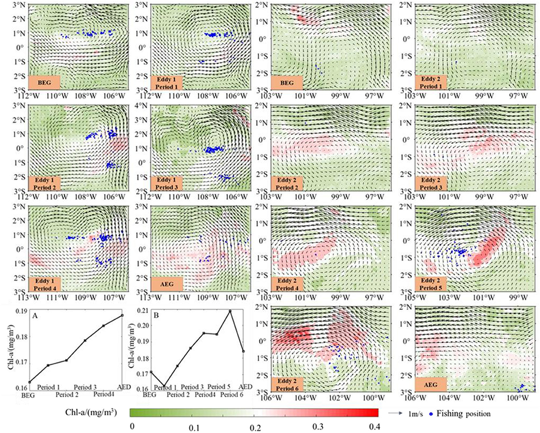
Figure 4. The effects of eddies 1 and 2 on chlorophyll-a (Chl-a) concentration on the fishing ground of D. gigas in the eastern equatorial Pacific Ocean. (A) (eddy 1) and (B) (eddy 2) show the variations of Chl-a concentration in different periods.

The Influences of the Eddy on D. gigas Abundance and Spatial Distribution

The variation trend of the number of eddies and average D. gigas CPUE from April to June was consistent (Figure 5A). The average CPUE in each month was 3.8 t/d in April, 4 t/d in May, and 3 t/d in June, respectively. The number of eddies and the CPUE changed synchronously.

FIGURE 5

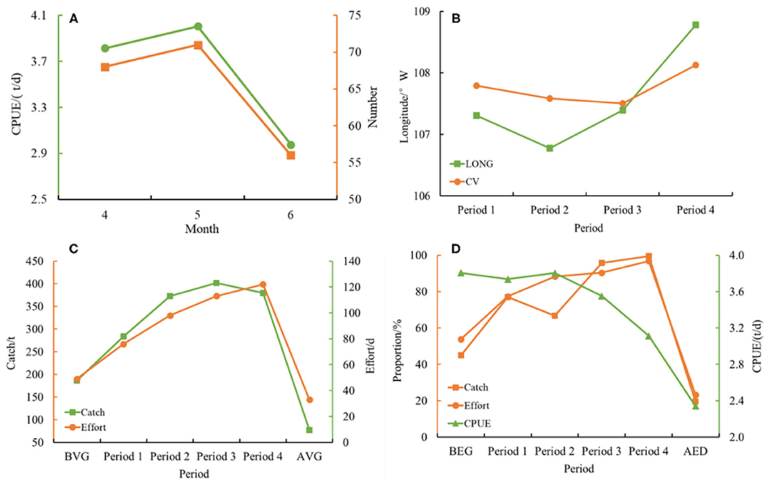
Figure 5. (A) Shows monthly variations of the number of eddies and the mean catch per unit effort (CPUE) from April to June 2017 on the fishing ground of D. gigas in the equator. (B) Shows the variations of the center of the eddy 1 and the longitudinal gravity center of fishing efforts (LONG) of D. gigas. The center of the eddy was determined based on the eddy-detecting model, and the LONG was calculated by the formula in section 2.3.2. (C) Shows the variations of the total catch and fishing efforts in different periods of eddy 1. (D) Shows the proportion of catch and fishing efforts of D. gigas in the whole study area and the variations of CPUE in the different periods of eddy 1.

The variations in the catch, fishing effort, and CPUE of D. gigas in each period of eddy 1 are shown in Figures 5C,D. The catch and fishing effort showed an increasing trend throughout the eddy lifetime. The catch increased from the initial 186.5 t (BEG) to approximately 400 t (period 3 and 4), and the fishing effort increased from the initial 42 times (BEG) to 122 times (period 4). The CPUE remained at a relatively high level (>3 t/d) from BEG to period 2, but it decreased in the next two stages (from periods 3–4). The proportions of the catch and fishing efforts around the eddy in the entire study area were increased, implying that increasing D. gigas individuals were gathered within eddy 1.

To determine the influences of the eddy on D. gigas distribution and the biophysical environment, the fishing positions in the equatorial waters were examined, and the different periods of eddy 1 were matched with them (Figures 3, 4). With high temperature and low Chl-a in the BEG, the D. gigas was distributed dispersedly in a straight line. The D. gigas gradually gathered to the center of the eddy in period 1 and shifted to the east side where SST was lower, and the Chl-a concentration was higher in period 2. With the continuous effect of the eddy, the low-temperature waters gradually spread westward, and the high Chl-a areas gradually became larger. To respond to changes in the environment, the D. gigas gradually migrated westward (period 3), and then gradually spread (period 4). Comparing the LONG and the center of the eddy, the movement patterns of these two parameters were almost stable (Figure 5B).

The Distribution of Suitable Habitats of D. gigas Within Eddy 1

The HSI model could predict the habitat suitability of D. gigas based on the results of the statistical analysis and model validation (Supplementary File 3). The spatio-temporal distribution of the suitable habitats of D. gigas in the different periods of eddy 1 is shown in Figure 6. Suitable habitats were distributed in the western and eastern waters in the study area in BEG. From periods 1–3 of eddy 1, the habitat suitability gradually increased, and the area of suitable habitat was distributed successively and gradually extended to the north and south. In periods 2 and 3, the habitat suitability in the eddy center positions increased significantly, while the suitable habitat in the southeast area of the eddy gradually increased. However, in period 4, suitable habitats were mainly distributed in the northeastern and southern waters of eddy 1, with a larger area of suitable habitats in the southern regions than in the northeastern areas. The suitable habitat was largely reduced, and only a part was scattered in the eastern waters in the AED. In addition, the average HSI and the proportion of suitable habitats in the eddy 1 first increased and then decreased. Both were the largest in period 3 (Figures 6A,B). There was a significant difference between HSI levels at period 3 and BEG of eddy 1 (t = 12.58, p < 0.01).

FIGURE 6

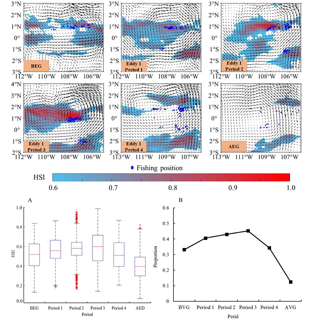
Figure 6. Distribution of suitable habitats in different periods of eddy 1. The arithmetic mean method (AMM)-based model was established with the relationship between the effort and environment factors (SST, Chl-a, Temp_50 m, and Temp_100 m). (A) Shows the variations of the average habitat suitability index (HSI) in the different periods of eddy 1. (B) Shows the proportion of suitable habitats in the whole area of eddy 1.

Discussion

The Mechanism of Eddy Generation

The generation of the mesoscale eddy is observed due to the instability of currents and wind stress curl (Holmes et al., 2014; Lin et al., 2015; Zheng et al., 2016). Because of the special geographic location and complex marine environmental elements, the causes of eddy formation are complicated in equatorial waters. There is a strong trade wind on the equatorial sea surface, blowing the North and South Equatorial Warm Currents westward to eastward (Brown et al., 2007). In addition, the equatorial waters have a complicated current system, reflecting the direction and strength of each tributary (Brown et al., 2007; Sen Gupta et al., 2012). Those environmental features drive the equatorial waters by intensive eddy activities. The baroclinic instability between both close tributaries was the main reason for the eddy formation (Figure 1) (Dutrieux et al., 2008; Zheng et al., 2016).

Our results showed that the lifetime of the eddy in the equatorial waters was shorter than those in other areas (Liu et al., 2012; Lin et al., 2015). One hundred ninety-five eddies were detected in the equatorial waters of the Eastern Pacific from April to June 2017, and 93% of them had a lifetime of <1 week. The reason may come from two aspects. The first one is the unique environment of the equatorial water and the generation mechanism of the eddy, and the second one is that the Coriolis force of the equatorial water is very small. Most of the eddies cannot maintain their shape but can migrate after the eddy formation.

The Impacts of Eddies on the Vertical Temperature Structure

Mesoscale oceanographic activities are ubiquitous in the ocean, and they are the important media that regulate the marine environment, transport marine materials, and change heat between the ocean and the atmosphere. These act as potential drivers that affect the biological environment (Dong et al., 2014; Gaube et al., 2014; Zhang et al., 2014). Eddies have a strong influence on water temperature structure in equatorial waters. In the horizontal direction, the anticyclonic eddy enhances the mixing of water masses at different temperatures, causing cold water to shift northward, with a southward movement of warm water. Thus, it forms a thermal front with a relatively large temperature gradient in the north equator (Flament et al., 1996; Kennan and Flament, 2000). In the vertical direction, the anticyclone eddy causes a thermocline decline, but the northern cold waters make the isotherm move upward and consequently form an upwelling (Kennan and Flament, 2000; Menkes et al., 2002). On the surface of the eddy, there was no obvious horizontal exchange of water masses at different temperatures (disturbance of the SST), and the location of the eddy can influence the horizontal exchange of water masses. The center of the anticyclonic eddy discovered by Flament was at 4°N in the middle between the North Equatorial Countercurrent (higher temperature) and the Equatorial Undercurrent (lower temperature) with the greater temperature gradient.

The two selected eddies in this study were characterized by an anti-clockwise rotation. Eddy 1 was cyclonic eddy, and the eddy 2 was anticyclonic eddy. The cyclonic eddy could form an upwelling raising the thermocline, and the anticyclone would push down subsurface waters and produce downwelling, with a decreased thermocline (McGillicuddy, 2016). Both eddies in this study had the same impacts on the vertical temperature structure (Figure 3) because they might have the same three-dimensional shape. Different shapes had different impacts on the vertical temperature structure for the cyclonic eddy (Lin et al., 2015). The cold water might come from North Equatorial Countercurrent and Equatorial Undercurrent (Dutrieux et al., 2008; Zheng et al., 2016), and the eddy close to the equator could form the Ekman pumping, leading to strong vertical water mixing by the upwelling.

The Influences of Eddies on the Chl-a Concentration

There are different dynamic mechanisms about how the mesoscale eddy affects the Chl-a, including horizontal eddy stirring, eddy trapping, and limiting eddy-induced Ekman pumping and eddy-wind interaction (Martin and Richards, 2001; Chen et al., 2013; Gaube et al., 2014; McGillicuddy, 2016). The differences in the physical, chemical, and biological characteristics around the eddy lead to various Chl-a concentration distribution patterns with different dynamic mechanisms. According to the intensity changes of the eddy, the entire lifetime of the eddy was divided into four periods, namely, formation, intensification, maturation, and extinction (Gaube et al., 2014; Xu et al., 2019). During the intensification and maturity periods, the ring-shaped Chl-a structure was more frequent and intense. This study also divided the entire lifetime of the eddy 1 into four periods, corresponding to formation, strengthening, maturation, and extinction (Supplementary File 1), to explore the environment variations under each period of the eddy (Figures 3, 4).

Based on previous studies, the eddy-induced Ekman pumping in the equatorial waters resulted in upwelling, transporting the subsurface cold water upward, and rising the isotherm. At the same time, it transported the nutrients to the light-transmitting layer for promoting plankton reproduction and Chl-a concentration. Figure 4 showed that the Chl-a concentration rose in the AED of eddy 1, and it might be caused by the unique geographic locations of the two eddies. The generation time and the distance (Supplementary File 1) of eddy 1 and 2 were close, and the joint interactive effects of the two eddies might have great impacts on the environment. For example, compared to the outer sides, the SST in the middle of the two eddies dropped rapidly, especially in the eddy center. The Chl-a increased significantly in the middle of the two eddies (Figure 4). When eddy 1 disappeared, eddy 2 shifted to the east side of eddy 1. Therefore, the persistent effects of eddy 2 might lead to the continuous rising of Chl-a concentration, but it decreased in the AED of the eddy 2.

The Influences of Eddy on the D. gigas Stock and Its Potential Mechanism

According to the movement patterns, the life cycle for short-lived squid species is divided into two stages: passive drifting and active migrating stages (Yu et al., 2015). The process by which eddy influences the distribution pattern of D. gigas in the equator can also be divided into two stages. The eddy can trap D. gigas in the early life stage, including planktonic egg mass and paralarvae phases, and transport them to the west from Peru and the Costa Rican Dome (Anderson and Rodhouse, 2001; Chen et al., 2012, 2013; Sanchez-Velasco et al., 2016). At the same time, eddies can attract latter stages of D. gigas, including juvenile, subadult, and mature adult, like other pelagic fishes (Flament et al., 1996; Willett et al., 2006).

This study showed that D. gigas in the equatorial waters gradually migrated to the southeastern waters from April to June, and the regions with the occurrence of short-lived eddies became a potential temporary habitat for D. gigas. As shown in Figure 7, our study inferred that the eddy-driven mechanism changed in the marine environment. It also induced the gathering of D. gigas by combing all the information together at the early stage of eddy (period 1). The intensity of the eddy-induced upwelling was weaker due to the low-intensity eddy. Only a small amount of subsurface water was pumped to the upper ocean, and the nutrient density was low. Relatively lower D. gigas abundance occurred in the eddy. With the increased intensity of the eddy (period 2), the upwelling intensity strengthened, and the vertical temperature fell. Large cold water mass rose, and more bottom nutrients were carried into the euphotic layer. The primary productivity then largely increased with the photosynthesis of phytoplankton. Subsequently, in period 3, the surface layer of nutrients increased plankton production, providing a favorable feeding environment and a high-quality habitat and attracting more D. gigas to gather in the eddy. With the extinction of the eddy (period 4), the upwelling intensity weakens, and the temperature and the nutrient density decreased. At the same time, the habitat quality became poorer, and the catch, fishing effort, and CPUE decreased. Our findings suggest that eddy activities have significant impacts on D. gigas abundance and habitat distribution.

FIGURE 7

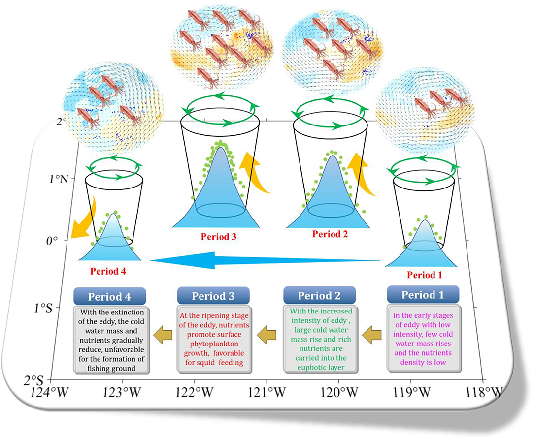
Figure 7. The influence mechanism of the equatorial eddy on physical and biological environments and the distribution and abundance of D. gigas in the eastern equatorial Pacific Ocean. The green arrow indicates the shifting direction of the eddy. The yellow arrow indicates the upwelling, and the dots indicate nutrients.

Data Availability Statement

The original contributions presented in the study are included in the article/Supplementary Material, further inquiries can be directed to the corresponding author.

Author Contributions

WY, XF, and XC conceptualized the study. WY, YZ, and XF designed the methodology and provided the software analyzed the data for the study. XF and WY wrote the original draft. WY and XC involved in the funding acquisition. The manuscript was written through contributions of all authors. All authors have given approval to the final version of the manuscript.

Funding

This study was financially supported by the National Key R&D Program of China (2019YFD0901405, 2019YFD0901404), the National Natural Science Foundation of China (41906073), and the Natural Science Foundation of Shanghai (19ZR1423000).

Conflict of Interest

The authors declare that the research was conducted in the absence of any commercial or financial relationships that could be construed as a potential conflict of interest.

Publisher's Note

All claims expressed in this article are solely those of the authors and do not necessarily represent those of their affiliated organizations, or those of the publisher, the editors and the reviewers. Any product that may be evaluated in this article, or claim that may be made by its manufacturer, is not guaranteed or endorsed by the publisher.

Supplementary Material

The Supplementary Material for this article can be found online at: https://www.frontiersin.org/articles/10.3389/fmars.2021.721291/full#supplementary-material

References

Anderson, C. I., and Rodhouse, P. G. (2001). Life cycles, oceanography and variability: ommastrephid squid in variable oceanographic environments. Fish. Res. 54, 133–143. doi: 10.1016/S0165-7836(01)00378-2

CrossRef Full Text | Google Scholar

Brown, J. N., Godfrey, J. S., and Schiller, A. (2007). A discussion of flow pathways in the central and eastern equatorial Pacific. J. Phys. Oceanogr. 37, 1321–1339. doi: 10.1175/JPO3042.1

CrossRef Full Text | Google Scholar

Chaigneau, A., Eldin, G., and Dewitte, B. (2009). Eddy activity in the four major upwelling systems from satellite altimetry (1992–2007). Prog. Oceanogr. 83, 117–123. doi: 10.1016/j.pocean.2009.07.012

CrossRef Full Text | Google Scholar

Chen, X. J., Li, J. H., Liu, B. L., Chen, Y., Li, G., Fang, Z., and Tian, S. Q. (2013). Age, growth and population structure of jumbo flying squid, Dosidicus gigas, off the Costa Rica Dome, Marine Biological Association of the United Kingdom. J. Mar. Biol. Assoc. UK. 93, 567–573. doi: 10.1017/S0025315412000422

CrossRef Full Text | Google Scholar

Chen, X. J., Li, J. H., Yi, Q., Liu, B. L., Yang, M. X., and Lu, H. J. (2012). Preliminary study on fisheries biology of Dosidicus gigas in the waters near the equator of eastern Pacific Ocean. Oceanol. Limnol. Sin. 43, 1233–1238. doi: 10.11693/hyhz201206029029

CrossRef Full Text

Chen, X. J., and Zhao, X. H. (2005). Catch distribution of jumbo flying squid and its relationship with SST in the offshore waters of Chile. Mar. Fish. 27, 173–176. doi: 10.3969/j.issn.1004-2490.2005.02.016

CrossRef Full Text | Google Scholar

Csirke, J., Alegre, A., Argüelles, J., Guevara-Carrasco, R., Mariátegui, L., Segura, M., et al. (2015). “Main biological and fishery aspects of the jumbo squid (Dosidicus gigas) in the Peruvian Humboldt Current System,” in 3rd meeting of the Scientific Committee of the SPRFMO, Port Vila, Vanuatu (Vol. 28).

Google Scholar

Davis, R. W., Ortega-Ortiz, J. G., Ribic, C. A., Evans, W. E., Biggs, D. C., Ressler, P. H., et al. (2002). Cetacean habitat in the northern oceanic Gulf of Mexico. Deep Sea Res. Part I: Oceanogr. Res. Pap. 49, 121–142. doi: 10.1016/S0967-0637(01)00035-8

CrossRef Full Text | Google Scholar

De Monte, S., Cotté, C., d'Ovidio, F., Lévy, M., Le Corre, M., and Weimerskirch, H. (2012). Frigatebird behaviour at the ocean–atmosphere interface: integrating animal behaviour with multi-satellite data. J. R. Soc. Interface 9, 3351–3358. doi: 10.1098/rsif.2012.0509

PubMed Abstract | CrossRef Full Text | Google Scholar

Dong, C. M., McWilliams, J. C., Liu, Y., and Chen, D. (2014). Global heat and salt transports by eddy movement. Nat. Commun. 5, 1–6. doi: 10.1038/ncomms4294

PubMed Abstract | CrossRef Full Text | Google Scholar

Dutrieux, P., Menkes, C. E., Vialard, J., Flament, P., and Blanke, B. (2008). Lagrangian study of tropical instability vortices in the Atlantic. J. Phys. Oceanogr. 38, 400–417. doi: 10.1175/2007JPO3763.1

CrossRef Full Text | Google Scholar

Fang, X. N, Yu, W., and Chen, X J. (2021). Spatial distribution of fishing ground of Dosidicus gigas in the equator in 2017. Fish. Sci. [Epub ahead of print].

Fernández-Álamo, M. A., and Färber-Lorda, J. (2006). Zooplankton and the oceanography of the eastern tropical Pacific: a review. Prog. Oceanogr. 69, 318–359. doi: 10.1016/j.pocean.2006.03.003

CrossRef Full Text | Google Scholar

Flament, P. J., Kennan, S. C., Knox, R. A., Niiler, P. P., and Bernstein, R. L. (1996). The three-dimensional structure of an upper ocean vortex in the tropical Pacific Ocean[J]. Nature, 383, 610–613. doi: 10.1038/383610a0

CrossRef Full Text | Google Scholar

Gaube, P., McGillicuddy Jr, D. J., Chelton, D. B., Behrenfeld, M. J., and Strutton, P. G. (2014). Regional variations in the influence of mesoscale eddies on near-surface chlorophyll. J. Geophys. Res. Oceans 119, 8195–8220. doi: 10.1002/2014JC010111

CrossRef Full Text | Google Scholar

Holmes, R. M., Thomas, L. N., Thompson, L., and Darr, D. (2014). Potential vorticity dynamics of tropical instability vortices. J. Phys. Oceanogr. 44, 995–1011. doi: 10.1175/JPO-D-13-0157.1

CrossRef Full Text | Google Scholar

Ibáñez, C. M., Sepúlveda, R. D., Ulloa, P., Keyl, F., and Pardo Gandarillas, M. C. (2015). The biology and ecology of the jumbo squid Dosidicus gigas (Cephalopoda) in Chilean waters: a review. Univ. Psychol. 43, 402–414. doi: 10.3856/vol43-issue3-fulltext-2

CrossRef Full Text | Google Scholar

Kai, E. T., and Marsac, F. (2010). Influence of mesoscale eddies on spatial structuring of top predators' communities in the Mozambique Channel. Prog. Oceanogr. 86, 214–223. doi: 10.1016/j.pocean.2010.04.010

CrossRef Full Text | Google Scholar

Kennan, S. C., and Flament, P. J. (2000). Observations of a tropical instability vortex. J. Phys. Oceanogr. 30, 2277–2301. doi: 10.1175/1520-0485(2000)030andlt;2277:OOATIVandgt;2.0.CO;2

CrossRef Full Text | Google Scholar

Keyl, F., Argüelles, J. U. A. N., Mariátegui, L. U. Í. S., Tafandur, R., Wolff, M., and Yamashiro, C. (2008). A hypothesis on range expansion and spatio-temporal shifts in size-at-maturity of jumbo squid (Dosidicus gigas) in the Eastern Pacific Ocean. CalCOFI Rep. 49, 119–128. doi: 10.1016/j.aquaculture.2008.07.038

CrossRef Full Text | Google Scholar

Lavín, M. F., Fiedler, P. C., Amador, J. A., Ballance, L. T., Färber-Lorda, J., and Mestas-Nuñez, A. M. (2006). A review of eastern tropical Pacific oceanography: summary. Prog. Oceanogr. 69, 391–398. doi: 10.1016/j.pocean.2006.03.005

CrossRef Full Text | Google Scholar

Lin, X. Y., Dong, C. M., Chen, D. K., Liu, Y., Yang, J. S., Zou, B., et al. (2015). Three-dimensional properties of mesoscale eddies in the South China Sea based on eddy-resolving model output. Deep Sea Res. Part I: Oceanogr. Res. Pap. 99, 46–64. doi: 10.1016/j.dsr.2015.01.007

CrossRef Full Text | Google Scholar

Liu, Y., Dong, C., Guan, Y. P., Chen, D. K., McWilliams, J., and Nencioli, F. (2012). Eddy analysis in the subtropical zonal band of the North Pacific Ocean. Deep Sea Res. Part I: Oceanogr. Res. Pap. 68, 54–67. doi: 10.1016/j.dsr.2012.06.001

CrossRef Full Text | Google Scholar

Martin, A. P., and Richards, K. J. (2001). Mechanisms for vertical nutrient transport within a North Atlantic mesoscale eddy. Deep Sea Res. Part II: Top. Stud. Oceanogr. 48, 757–773. doi: 10.1016/S0967-0645(00)00096-5

CrossRef Full Text | Google Scholar

McGillicuddy, D. J. Jr (2016). Mechanisms of physical-biological-biogeochemical interaction at the oceanic mesoscale. Annu. Rev. Mar. Sci. 8, 125–159. doi: 10.1146/annurev-marine-010814-015606

PubMed Abstract | CrossRef Full Text | Google Scholar

Menkes, C. E., Kennan, S. C., Flament, P., Dandonneau, Y., Masson, S., Biessy, B., et al. (2002). A whirling ecosystem in the equatorial Atlantic. Geophys. Res. Lett. 29, 48–54. doi: 10.1029/2001GL014576

CrossRef Full Text | Google Scholar

Nencioli, F., Dong, C., Dickey, T., Washburn, L., and McWilliams, J. C. (2010). A vector geometry–based eddy detection algorithm and its application to a high-resolution numerical model product and high-frequency radar surface velocities in the Southern California Bight. J. Atmos. Ocean. Technol. 27, 564–579. doi: 10.1175/2009JTECHO725.1

CrossRef Full Text | Google Scholar

Penven, P., Echevin, V., Pasapera, J., Colas, F., and Tam, J. (2005). Average circulation, seasonal cycle, and mesoscale dynamics of the Peru Current System: a modeling approach. J. Geophys. Res.Oceans. 110:C10021. doi: 10.1029/2005JC002945

CrossRef Full Text | Google Scholar

Sanchez-Velasco, L., Ruvalcaba-Aroche, E. D, Beier, E, Godinez, V. M, Barton, E. D, Diaz-Viloria, N, and Pacheco, M. R. (2016). Paralarvae of the complex Sthenoteuthis oualaniensis-Dosidicus gigas (Cephalopoda: Ommastrephidae) in the northern limit of the shallow oxygen minimum zone of the Eastern Tropical Pacific Ocean (April 2012). J. Geophys. Res. Oceans. 121, 1998–2015. doi: 10.1002/2015JC011534

CrossRef Full Text

Sen Gupta, A., Ganachaud, A., McGregor, S., Brown, J. N., and Muir, L. (2012). Drivers of the projected changes to the Pacific Ocean equatorial circulation. Geophys. Res. Lett. 39:L09605. doi: 10.1029/2012GL051447

CrossRef Full Text | Google Scholar

Willett, C. S., Leben, R. R., and Lavín, M. F. (2006). Eddies and tropical instability waves in the eastern tropical Pacific: a review. Prog. Oceanogr. 69, 218–238. doi: 10.1016/j.pocean.2006.03.010

CrossRef Full Text | Google Scholar

Xu, G. J., Dong, C. M., Liu, Y., Gaube, P., and Yang, J. S. (2019). Chlorophyll rings around ocean eddies in the North Pacific. Sci. Rep. 9, 1–8. doi: 10.1038/s41598-018-38457-8

PubMed Abstract | CrossRef Full Text | Google Scholar

Yi, Q., Chen, X. J, Liu, B L., Yu, W., Li, J. H., and Fang, Z. (2014). A comparison of habitats of Dosidicus gigas in the fishing ground off Chile and Peru based on information gain technique. J. Shanghai Ocean Univ. 23, 272–278.

Yu, W., Chen, X. J., Yi, Q., and Tian, S. Q. (2015). A review of interaction between neon flying squid (Ommastrephes bartramii) and oceanographic variability in the North Pacific Ocean. J. Ocean Univ. China. 14, 739–748. doi: 10.1007/s11802-015-2562-8

CrossRef Full Text | Google Scholar

Yu, W., Wen, J., Chen, X., Gong, Y., and Liu, B. (2021). Trans-Pacific multidecadal changes of habitat patterns of two squid species. Fish. Res. 233:105762. doi: 10.1016/j.fishres.2020.105762

CrossRef Full Text | Google Scholar

Yu, W., Yi, Q., Chen, X. J., and Chen, Y. (2016). Modelling the effects of climate variability on habitat suitability of jumbo flying squid, Dosidicus gigas, in the Southeast Pacific Ocean off Peru. ICES J. Mar. Sci. 73, 239–249. doi: 10.1093/icesjms/fsv223

CrossRef Full Text | Google Scholar

Yu, W., Yi, Q., Chen, X. J., and Chen, Y. (2017). Climate-driven latitudinal shift in fishing ground of jumbo flying squid (Dosidicus gigas) in the Southeast Pacific Ocean off Peru. Int. J. Remote Sens. 38, 3531–3550. doi: 10.1080/01431161.2017.1297547

CrossRef Full Text | Google Scholar

Zhang, Z. G., Wang, W., and Qiu, B. (2014). Oceanic mass transport by mesoscale eddies. Science 345, 322–324. doi: 10.1126/science.1252418

PubMed Abstract | CrossRef Full Text | Google Scholar

Zheng, S. J., Feng, M., Du, Y., Cheng, X. H., and Li, J. X. (2016). Annual and interannual variability of the tropical instability vortices in the equatorial eastern Pacific observed from Lagrangian surface drifters. J. Clim. 29, 9163–9177. doi: 10.1175/JCLI-D-16-0124.1

CrossRef Full Text | Google Scholar