The Wind Effect on Biogeochemistry in Eddy Cores in the Northern South China Sea

Cyclonic and anticyclonic eddies are usually characterized by upwelling and downwelling, respectively, which are induced by eddy pumping near their core. Using a repeated expendable bathythermograph transect (XBT) and Argo floats, and by cruise experiments, we determined that not all eddies in the northern South China Sea (NSCS) were accompanied by eddy pumping. The weakening of background thermocline was attributed to the strengthening of eddy pumping, affected by (1) wind-induced meridional Sverdrup transports and (2) Kuroshio intrusion into the NSCS. Higher particulate organic carbon (POC) fluxes (> 100 mg-C m⁻² day⁻¹) were found near the eddy cores with significant eddy pumping (defined by a depth change of 22°C isotherm near the thermocline for over 10 m), although the satellite-estimated POC fluxes were inconsistent with the in-situ POC fluxes. nitrogen limitation transition and high POC flux were even found near the core of a smaller mesoscale (diameter < 100 km) cyclonic eddy in May 2014, during the weakening of the background thermocline in the NSCS. This finding provides evidence that small mesoscale eddies can efficiently provide nutrients to the subsurface, and that they can remove carbon from the euphotic zone. This is important for global warming, which generally strengthens upper ocean stratification.

Introduction

The Southeast Asia monsoon largely determines the ocean circulation in the South China Sea (SCS), the largest semi-closed marginal sea in the northwest Pacific. During the northeast (NE) monsoon, ocean circulation is mainly occupied by a basin-wide cyclonic gyre in the upper layer of the SCS (Su, 2004), with Kuroshio intrusion through the Luzon Strait (Hu et al., 2000; Nan et al., 2015). In general, the Kuroshio intrudes warmer and saltier water from the Pacific into the northern SCS (NSCS). During the southwest (SW) monsoon, ocean circulation is characterized by two basin-wide gyres in the upper layer of the SCS: one is cyclonic in the NSCS, and the other is anticyclonic in the southern South China Sea (SSCS) (Su, 2004).

According to in situ and satellite observations, the seawater in the region of the SCS basin is strongly stratified and oligotrophic, with a low chlorophyll-a (Chl) concentration (< 0.1 mg/m³) near the surface (Liu et al., 2002; Chen, 2005; Chen et al., 2006; Shen et al., 2008; Zhang et al., 2016). Phytoplankton growth near the surface is limited because of nearly undetectable nitrogen concentration, corresponding to the deep nitracline (Liu et al., 2002; Chen et al., 2004, 2006; Zhang et al., 2016). However, in the region of the basin, during the NE monsoon, surface Chl concentration can reach as high as 0.3 mg/m³ (Liu et al., 2002; Shen et al., 2008). This is because the shallower nitracline causes an increase in nitrate-based new production (Chen, 2005). Physical factors that support phytoplankton growth in marginal seas include monsoons (Liu et al., 2002), dust deposition (Wu et al., 2003; Hung et al., 2009), typhoons (Siswanto et al., 2007, 2008; Hung et al., 2010b; Chen et al., 2013; Shih et al., 2013, 2020), ocean eddies (Chen et al., 2007, 2015; Shih et al., 2015), and internal waves (Li et al., 2018a; Tai et al., 2020). These provide nutrient supplies in the sunlit layer via surface fluxes, horizontal advection, vertical upwelling, and vertical mixing.

The South China Sea is full of ocean mesoscale eddies (Hwang and Chen, 2000; Wang et al., 2003; Chow et al., 2008; Xiu et al., 2010; Du et al., 2016; Chu et al., 2020), which have a mean radius of ~132 km and a lifetime of ~8.8 weeks (Chen et al., 2011). Ocean cooling and warming can form near the core of cyclonic eddies (CEs) and anticyclonic eddies (AEs), respectively, induced by eddy pumping (Soong et al., 1995; Li et al., 1998; Chow et al., 2008; Xiu and Chai, 2011). However, eddy-induced cooling and warming were not found universally in mesoscale eddies near the ocean surface. Liu et al. (2020) found that only ~60% of AEs and CEs corresponded to the positive and negative anomalies of sea surface temperature (SST), respectively, based on satellite observation of the SCS. Namely, ~40% of eddies had warm-core CEs and cold-core AEs, reversed to a generally known situation that CEs and AEs are usually characterized by cold and warm cores, respectively. Indeed, warm-core CEs and cold-core AEs have been detected in the Pacific and the Atlantic using a satellite and by in-situ observation (Flagg et al., 1998; Itoh and Yasuda, 2010; Shih et al., 2015; Sun et al., 2019). Huang and Xu (2018) suggested that when studying eddy-related biogeochemistry by satellite observation, the upper-ocean vertical structure should be carefully considered. Subsurface Chl variability cannot be fully detected from the surface via satellite measurements in mesoscale eddies.

Cold-core cyclonic eddies and warm-core anticyclonic eddies can contribute to local biogeochemical budgets via strong vertical upwelling (Chen et al., 2007) and deep vertical mixing (Chen et al., 2015), respectively. The mechanisms of global eddy-induced Chl variation can be classified into several types (Siegel et al., 2011; McGillicuddy, 2016): (1) eddy pumping (a general type), (2) eddy-wind interaction (eddy-Ekman pumping), (3) eddy stirring/advection (Chelton et al., 2011a; Chow et al., 2017), (4) strain-induced submesoscale upwelling along eddy peripheries (McGillicuddy, 2016; Chow et al., 2019; Zhang et al., 2019), (5) eddy trapping (McGillicuddy, 2016), and (6) eddy-induced mixed-layer deepening (Gaube et al., 2014; McGillicuddy, 2016). Moreover, high fluxes of particulate organic carbon (POC), ranging from 83 to 194 mg-C m⁻²day⁻¹, were observed around the eddies in the western North Pacific (Shih et al., 2015). In the SCS, eddy currents were found to be controlling the particle movement within eddies. With a sinking rate of below 80 m day⁻¹, particles can be transported from the eddy edge to the eddy core (Ma et al., 2021).

In this study, we observed the ocean vertical structure in several mesoscale eddies by analyzing the ocean profiles obtained via expendable bathythermographs (XBTs), Argo floats, and cruise measurements. We found that not all eddies were accompanied by eddy pumping. What was the condition required for significant eddy pumping near the core of eddies in the NSCS? What was the biogeochemical response to eddies with and without eddy pumping? To answer these scientific questions, we studied the variability in the ocean vertical structure, nutrients, and POC flux corresponding to eddies in the NSCS, where the temperature-salinity (TS) properties of seawater are largely affected by ocean currents from its boundary, such as the Kuroshio intrusion. We defined the significant eddy pumping in the Data and Methods section. Then, we showed the significant eddy pumping that is related to the weakening of ocean stratification, combined with the results of nutrient dynamics, POC flux, and wind-related mechanisms. Last, we showed that the Kuroshio intrusion may depress the eddy pumping.

Data and Methods

Ocean Profile Data

To observe the vertical motion near the eddy cores, we used the temperature-profile data, provided by the Coriolis Operational Oceanography, of expendable bathythermographs (XBTs) along the PX44 transect (shown by the black dots in Figure 1) that repeatedly passed through the northern South China Sea (NSCS) from 2000 to 2010 (43 transects of PX44). In addition, we applied the available hydrographic data of Argo floats from 2005 to 2017 that were collected and made available by the Coriolis Operational Oceanography. There were a total of 109 Argo floats found. We only used those flagged as good-quality Argo data of temperature, salinity, and pressure from eddy cores in the basin of the NSCS, where the ocean bottom is over 1,000 m. The Argo data selected in this study had a time resolution ranging from 3 to 4 days.

FIGURE 1

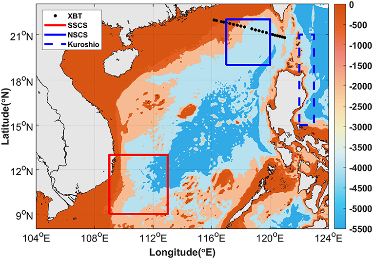
Figure 1. Bathymetry in the South China Sea (SCS). The black dots show the PX44 transect, which is the repeated hydrographic surveys of expendable bathythermographs (XBTs). The solid blue, dashed blue, and solid red rectangles show the region of northern South China Sea (NSCS), Kuroshio, and southern South China Sea (SSCS) used to show the long-term temperature-salinity (TS) properties of seawater.

To study the background temperature and salinity fields, assuming there were no eddy effects, we used the dataset from synoptic monthly gridded three-dimensional World Ocean Database version 2013 (WOD13) (Chu and Fan, 2017) and World Ocean Atlas version 2013 (WOA13), at 1° resolution, provided by the National Oceanic and Atmospheric Administration (NOAA). The monthly dataset of the former was available from 1945 to 2014. The anomalies of ocean profiles analyzed in this study were defined by referring to deviations from climatological means, which were obtained from WOA13. The WOA dataset included the 1°-gridded climatological profiles of temperature, salinity, and nutrients, which were linearly interpolated to the locations of the Argo floats and the stations of cruise measurements. Note that the results obtained in this study show no significant difference when the dataset of World Ocean Atlas version 2018 (WOA18) was used.

Eddy Detection

To detect the ocean eddies, we used the daily satellite-altimetry data of sea-level anomalies (SLAs) at 1/4° resolution obtained from the Copernicus Marine Environment Monitoring Service (CMEMS), available since the end of 1992. We derived the geostrophic velocity anomalies (u′, v′) from the zonal and meridional gradients of the daily SLAs (Hwang and Chen, 2000). Then, we calculated the Okubo–Weiss (OW) parameter (Okubo, 1970; Weiss, 1991; Faghmous et al., 2015) from the derived geostrophic velocity anomalies (u′, v′) using

$\begin{array}{ll}OW={S_{sh}}^2+{S_{st}}^2-\xi {}^2\dots & (1)\end{array}$

where S_sh is the shear deformation rate estimated as ∂v′/∂x + ∂u′/∂y, S_st is the stretch deformation rate estimated as ∂u′/∂x − ∂v′/∂y, and ξ is the current vorticity estimated as ∂v′/∂x − ∂u′/∂y.

The general flow in eddies is characterized by rotation, namely, a large magnitude of vorticity, around a background circulation (such as the SCS circulation or the Kuroshio intrusion) with flow dominated by the shear and stretch deformations. The OW parameter compares the deformation-dominated circulation (OW > 0) with the rotation-dominated eddies (OW < 0). Thus, in this study, we identified the ocean eddies according to the negative OW parameter at the local maxima and minima of two-dimensional SLAs, which could also be induced by background circulation (Chow et al., 2015) or planetary Rossby waves (Chelton et al., 2011b).

To study the eddy vertical structure obtained from the ocean profiles of the Argo floats and XBTs, the daily gridded values of SLAs and OW parameter were linearly interpolated onto the profile locations that passed through the eddy cores. If the profile locations were in the closed SLA contours with a negative OW parameter near the eddy cores (Ma et al., 2021), then we assumed that the ocean profiles were in the region of eddy cores, which were defined by the local maxima and minima of two-dimensional SLAs for the AEs and CEs, respectively (Faghmous et al., 2015). We used the MATLAB program for eddy detection written by Faghmous et al. (2015) to detect eddy cores. If the distance between the profile location and the eddy core was shorter than the length of the eddy minor axis, which was an eddy parameter provided by eddy detection codes (Faghmous et al., 2015), an ocean profile was confirmed to pass through an eddy core. We studied the eddy vertical structure observed with at least three ocean profiles, which were measured by an Argo float or along an XBT transect.

In this study, we included new-born/short-lived eddies that could be traced back for at least 10 days and were confirmed with the negative OW parameter (Supplementary Figures S1, S2). Globally, ~55% of eddies were short lived (<30 days) ones (Chen and Han, 2019), highlighting the considerable effects of short-lived eddies on the variability in marine environments. However, we excluded the eddies with a lifetime shorter than 10 days because of the higher uncertainty of eddy detection using satellite altimeters (Faghmous et al., 2015). Note that the misclassification rate for eddies with a 10-day-lifetime can reach up to 7% of global satellite-detected eddies. Overall, we analyzed the ocean profiles of six repeated-XBT transects (14% of 43 transects) and 10 Argo floats (9% of 109 Argo floats) that passed through the eddy cores (Supplementary Figures S1, S2) based on the above criteria.

Additionally, we used the satellite dataset of Chl concentration, SST, and surface wind. The Chl data were the daily interpolated cloud-free glob-color product, at a spatial resolution of 4 km, provided by the CMEMS. The SST and wind data were the daily product of microwave optimally interpolated (OI) SST and cross-calibrated multi-platform (CCMP) gridded surface vector winds, at a spatial resolution of 0.25°, provided by Remote Sensing Systems (RSS).

Eddy Pumping and Ocean Vertical Structure

To confirm eddy pumping near the eddy cores, we studied the profiles of XBTs and Argo floats that passed through the eddy cores, detected with the satellite altimeters. We defined the significant upwelling and downwelling of eddies according to the 22°C in situ isothermal depth (hereafter, D22) that varies at least 10 m upward and downward, respectively, from the depth of a climatological 22°C isotherm. The significant upwelling and downwelling were confirmed by two to four ocean profiles with a 10-m departure of D22 from the climatology.

Based on the repeated XBT transects, we found two anticyclonic eddies (AEs) and four cyclonic eddies (CEs) (AE1, AE4, and CE8 to CE11 in Supplementary Table S1). For Argo observation, we identified four AEs and six CEs. Supplementary Table S1 includes the dates of when the ocean profiles were closest to the eddy cores and the World Meteorological Organization (WMO) numbers of the Argo floats and XBT transects. The Argo floats are identified by their WMO numbers, hereafter. Interestingly, Argo 2900825 passed through the same anticyclonic eddy (AE1) observed along the XBT-WDD6033 transect in September 2008. Moreover, Argo 2901123 and Argo 2901382 co-observed the vertical profile of AE2 in December 2010. Argo 5902165 passed through the same CE5 observed during a cruise experiment in May 2014 (Supplementary Figure S3B). Two cruises were conducted onboard the R/V Ocean Researcher V (OR-V 0038) and R/V Ocean Researcher III (OR-III 1679) from 20th to 28th May 2014 and 14th to 17th April 2013, respectively (Shih et al., 2020). The former cruise (OR-V 0038) was along 116.2°E within 19°N and 18°N, observing CE5 with significant upwelling. While the latter cruise (OR-III 1679) was along 120.33°E within 22°N and 20°N, observing CE6 but without significant upwelling. Information on all eddy cases with and without significant eddy pumping is given in Supplementary Table S1.

We compared the biogeochemistry obtained between the two cruises. Water samples were collected together with CTD casts at Stations S1 and S2 for OR-III 1679, and Stations S3 and S4 for OR-V 0038 (Supplementary Figures S3A,B). To measure the concentration of nitrate + nitrite (N), phosphorus (P), and Chl from the water samples, we used the methods described in Shih et al. (2020). We also used the TS data provided by the ocean data bank (ODB) of Taiwan and from Argo 2901180, to study the TS properties of seawater near the XBT transects, which did not measure ocean salinity.

To observe ocean vertical structure in the time and space domain, we combined the ocean profiles obtained from the Argo floats, XBTs, and CTD casts near and around the eddy cores by calculating the squared buoyancy frequencies (N²) using (Gill, 1982).

$\begin{array}{ll}{N}^2=-\frac{g}{{\rho }_0}\frac{\partial \rho }{\partial z}\dots & (2)\end{array}$

where ρ is the ocean potential density, z is the depth (positive upward), ρ₀ is the mean ocean potential density between each depth, and g is gravity acceleration (=9.8 m/s²). To study the background ocean stratification, the average of squared buoyancy frequencies was calculated from the mixed-layer depth at ~50 m to the thermocline bottom at ~162 m (Peng et al., 2018).

Since expendable bathythermograph transects do not measure salinity, we reconstructed the salinity profiles at the stations of XBTs using the method of Vignudelli et al. (2003). We interpolated the TS profiles of WOD13 into the grids of XBT temperature data. Then, the WOD13 salinity in which the corresponding WOD13 temperature is closest to the XBT temperature was taken as salinity at the grids of the XBT temperature. We tested the salinity-reconstructed method using the temperature profile of Argo 2900825 near the core of AE1, comparing it with the salinity observed by the Argo float itself. For the salinity profile near the eddy core on September 28, 2008, the correlation coefficient between the reconstructed and observed salinity was ~0.98, with a root-mean-squared error of ~0.09 psu, showing acceptable performance of the salinity reconstruction method.

To study the effect of wind on oceanic variability, we further calculated the meridional Sverdrup transport (M_y), based on the CCMP wind product, using

$\begin{array}{ll}{M}_y=\frac{cur{l}_z\overrightarrow{\tau }}{\beta }=\frac{R}{2\Omega cos\phi }\left(\frac{\partial \overline{{\tau }_y}}{\partial x}-\frac{\partial \overline{{\tau }_x}}{\partial y}\right)\dots & (3)\end{array}$

In Equation (3), β is the change rate of coriolis force (f) due to latitude (∂f/∂y), R is the earth radius (= 6371 km), Ω is earth rotation angular speed (= 7.29 × 10⁻⁵ s⁻¹), φ is the latitude, and $cur{l}_z\overrightarrow{\tau }$ is the curl of the wind-stress vector $\overrightarrow{\tau }(\overline{{\tau }_x},\overline{{\tau }_y})$. In this study, $(\overline{{\tau }_x},\overline{{\tau }_y})$ was calculated using

$\begin{array}{ll}{\bar{\tau }}_x={\rho }_a\times C_d\times sp{d}_w\times u_w\dots & (4)\end{array}$

$\begin{array}{ll}{\bar{\tau }}_y={\rho }_a\times C_d\times sp{d}_w\times v_w\dots & (5)\end{array}$

$\begin{array}{ll}{C}_d=\frac{2.7}{sp{d}_w}+0.142+0.0764\times sp{d}_w\dots & (6)\end{array}$

where the air density ${\rho }_a=1.2\mathrm{\text{kg/}}{\mathrm{\text{m}}}^{\mathrm{\text{3}}}$, spd_w is the wind speed, and C_d is the drag coefficient, which was computed by following, Large and Pond (1982).

Measurement of POC Fluxes Near Eddy Cores

The particulate organic carbon fluxes were obtained near the eddy cores by in situ observation and satellite estimation. For in situ observation, we used buoy-tethered drifting sediment traps at ~150 m to collect sinking particles at cyclonic eddies in 2013 and 2014. The detailed method of buoy-tethered drifting traps can be found in Shih et al. (2019). Next, we followed the procedure of a POC analysis described by Shih et al. (2020) to determine the POC fluxes (Hung et al., 2010a) after collection from the traps. For satellite-derived POC flux estimation, we used the method given by Dunne et al. (2005):

$\begin{array}{l}{F}_{POC}=NPP\times \\ \left[-0.0101°C^{-1}\times SST+0.0582\times ln\left(\frac{NPP}{Z_{eu}}\right)+.419\right]\dots & (7)\end{array}$

where Z_eu is euphotic depth, and NPP is net primary production, which can be obtained via the satellite-derived vertically generalized production model (VGPM) first described by Behrenfeld and Falkowski (1997). Note that the VGRM assumed a homogeneous vertical distribution of Chl in the euphotic zone (Behrenfeld and Falkowski, 1997).

Results

Significant and Insignificant Eddy Pumping

This section represents the significant and insignificant eddy pumping observed via XBTs, Argo floats, and cruises, sequentially. Figure 2 shows the temperature profiles obtained via the XBT transect passing through the AEs in September of 2000 (AE4) and 2008 (AE1), and the CEs in April 2000 (CE8) and July 2009 (C10). As shown in Figure 2A, the downwelling is significant with the increase in D22 reaching 50 m (from 100 to 150 m) near the core of AE1. However, as shown in Figure 2C, no significant downwelling is observed near the core of AE4, according to the small changes in D22 (< 10 m), which are insignificant. For the satellite-detected CEs, Figure 2B shows the significant upwelling in CE8 according to D22 shallowing to 50 m. The outcropping of the isotherm can be seen near the surface in the eddy core, confirming the occurrence of upwelling. However, no significant upwelling can be found in the other three CE cases (CE9, CE10, and CE11) along the XBT transect (only CE10 is shown in Figure 2D, similar results were obtained for CE9 and CE11).

FIGURE 2

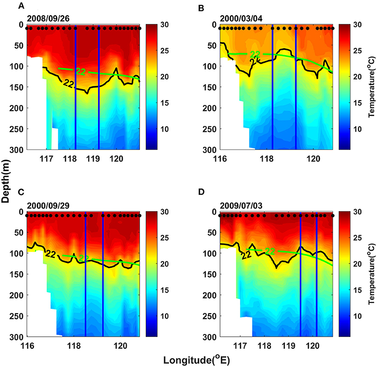
Figure 2. The temperature profiles along the PX44 section on (A) September 26, 2008 (AE1), (B) March 4, 2000 (CE8), (C) September 29, 2000 (AE4), and (D) July 3, 2009 (CE10). The two blue vertical lines in each sub-figure show the region within an eddy confirmed with satellite altimeters. The green curves show the climatological temperature contours at 22°C. The dots near the surface show the locations of expendable bathythermographs (XBTs). The left (right) panel is for the cases of anticyclonic (cyclonic) eddies, while the upper (lower) panel is for the cases with (without) significant eddy pumping.

Based on Argo observation, Figure 3 shows the temporal variation of ocean profiles in the AE1 observed along the XBT transect in September 2008. The significant downwelling can be seen from the Argo-obtained temperature profiles, represented by the increase in D22 reaching 50 m (from 100 to 150 m) from September 20 to November 6, 2008, when observing the AE1 profiles (Figure 3A). Note that D22 is shallower than the climatological field from one of the profiles on October 13, 2008 (Figure 3A), likely because of a different natural phenomenon with a shorter time scale, such as internal waves. Figure 3B also shows the relative variation in ocean stratification represented by N² anomalies. The negative N² anomalies can be found above 100 m (Figure 3B), showing a weaker stratification in the upper ocean. More studies exploring the weaker ocean stratification are given in Upper ocean stratification in the eddy cores Section.

FIGURE 3

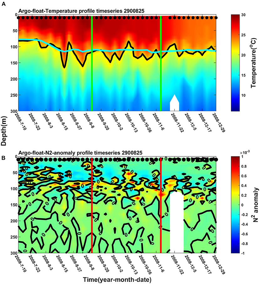
Figure 3. Profiles of (A) temperature and (B) N² anomalies obtained from Argo 2900825 from July 10 to December 29, 2008. The two vertical lines in each subfigure show the region of anticyclonic eddy confirmed with satellite altimeters. The dots near the surface show the observed times of the Argo float.

For all the Argo-observed ocean profiles corresponding to significant and insignificant eddy pumping, Figure 4 displays the temperature and temperature anomaly profiles near the eddy cores obtained with the 10 Argo floats used in this study (Supplementary Table S1). Figures 4A,C show the significant downwelling and upwelling, respectively, with a change in D22 over 10 m confirmed by two vertical profiles observed with each Argo float. In Figures 4B,D, the magnitude of temperature anomalies can reach as high as 4°C near the thermocline, showing a deeper and shallower depth of local maximum changes in temperature for the downwelling and upwelling, respectively. Similar results were obtained by Sun et al. (2018) who showed that the local maximum changes in density could be found within 50 and 110 m. For the cases with insignificant eddy upwelling, Figure 4E shows that D22 is similar to that of the climatological field, even with warming at some depths of observed CEs via Argo 2902045 and Argo 5902167 (Figure 4F). For the case observed via Argo 2900618, since there was only one profile that observed the changes in D22 over 10 m, it was not considered as significant eddy upwelling to avoid confusion with other natural phenomena.

FIGURE 4

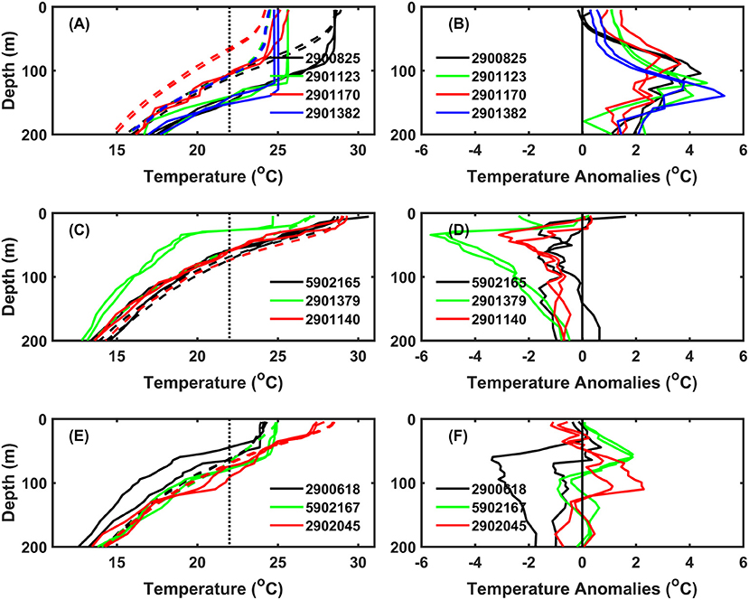
Figure 4. Profiles of temperature (left) and temperature anomalies (right) observed via Argo floats near the eddy cores for the cases of (A,B) anticyclonic eddies with significant downwelling, (C,D) cyclonic eddies with significant upwelling, and (E,F) cyclonic eddies without significant upwelling. The dashed curves in the left panel show the climatological temperature profiles corresponding to the Argo profiles in the same month. The vertical dotted line in the left panel shows the temperature at 22°C.

For the cruise experiments, Figure 5 shows the significant and insignificant upwelling in CE5 and CE6, respectively, which are characterized by the trough of sea-level anomalies (SLAs) along the cruise section (Figures 5A,B; Supplementary Figures S3A,B). Note that CE5 is a smaller eddy compared with the others in this study. However, in CE5, denser water (density maximum changes) can be found especially around 100 m near Station S4, compared with the surroundings (Figure 5C). In contrast to CE5, the maximum changes in ocean density were not found around 100 m near the core of CE6 (Figure 5D) but in the north boundary of CE6 near Station S1. Figures 5C,D show a large difference in ocean stratification between these two cases. Denser water is below 100 m in CE6 (Figure 5D), being depressed by lighter water from the surface to ~50 m. Thus, stronger stratification can be found within 50 to 100 m around CE6 (Figure 5F), in contrast to the weaker stratification around CE5 (Figure 5E). Moreover, no surface cooling can be detected in CE5 and CE6 along the cruise section via satellites (Figures 5A,B).

FIGURE 5

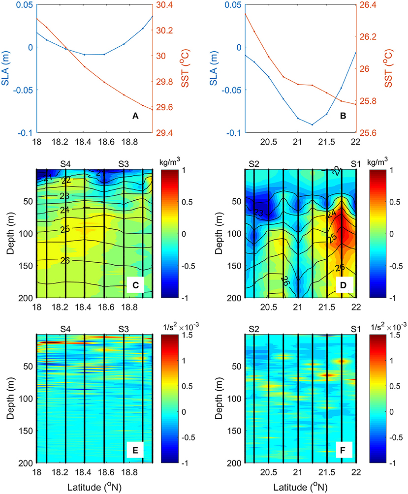
Figure 5. (A,B) Sea-level anomaly (SLA), sea surface temperature (SST), (C,D) density anomalies, and (E,F) N² anomalies observed along 116.17°E within 18°N and 19°N from May 20 to 28, 2014 (left) and along 120.33°E within 22°N and 22°N from April 14 to 17, 2013 (right). The stations, with water sample collection, are noted by “S1,” “S2,” “S3,” and “S4.” Contours in (C) and (D) show the density profiles.

Observed Biogeochemical Variability

Figure 6 shows the profiles of Chl, N, P, Si, N:P ratio, and Si:N ratio at Stations S1 and S2 near CE6, and Stations S3 (located at edge between CE5 and an AE) and S4 near CE5 during the cruise experiments. More nutrients are found at Stations S2 (green) and S4 (purple), compared with the climatological fields. However, Station S4 is closer to the core of CE5, while Station S2 is farther from the core of CE6. At Station S4, the depth of subsurface Chl maximum (SCM) is as shallow as 50 m (Figure 6A, purple), while the SCM depth at Station S3 (red) is deeper (75 m), indicating that the nutrient-rich water was upwelled toward the surface at Station 4 (Hung et al., 2003). The N and Si concentration at Station S4 is at least twice larger than the climatological profiles, reaching 10 and 11.6 μM, respectively, at 75 m (Figures 6B,D). In Figure 6E, the N:P ratios are generally smaller than 16:1 based on the climatological fields in the NSCS, highlighting the limitation of N. In contrast, at Station S4 near the CE5 core, the N:P ratios are larger than 16:1 at depths near the surface, reflecting the fact that P concentrations are insufficient to support phytoplankton growth (Figure 6E); while the Si:N ratios are maintained at 1~2 near the surface (Figure 6F).

FIGURE 6

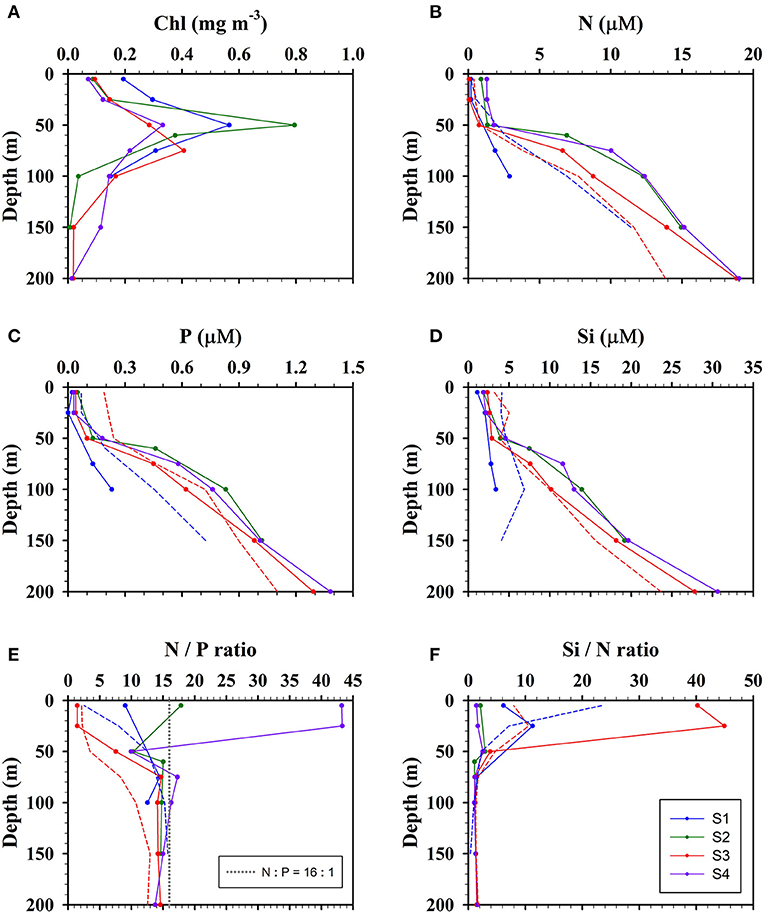
Figure 6. The concentration profiles of (A) chlorophyll-a (Chl), (B) nitrate + nitrite (N), (C) phosphate (P), (D) silicate (Si), (E) N:P ratio and (F) Si:N ratio, observed at Stations S1 (blue) and S2 (green) from April 14 to 17, 2013 and at Stations S3 (red) and S4 (purple) from May 20 to 28, 2014. Blue and red dashed curves show the relative climatological profiles for April and May, respectively, obtained from WOA13.

What potential mechanisms result in low Chl values at Stations 3 and 4 (i.e., near CE5)? The Chl concentration is ~0.33 mg m⁻³ at 50 m at Station 4 (the core of CE5), lower than that at Station 3 (~0.41 mg m⁻³). Previously, it has been shown that the warm and P-depleted water at Stations 3 and 4 were mainly from the mixed water of SCS and Kuroshio, based on the TS diagram (see Figure 1D from Shih et al., 2020). Shih et al. (2020) observed diatoms that are the predominant phytoplankton assemblages in the surface water near the CE5 core and reported that both POC flux (166 mg m⁻² day⁻¹) and diatom inventory (56 × 10⁶ cells m⁻²) at Station 3 were higher than those (POC flux = 50 mg m⁻² day⁻¹ and diatoms = 26 × 10⁶ cells m⁻²) at Station 4. These results suggest that various phytoplankton species and their cellular fluorescence signals may affect Chl inventories and POC fluxes (Shih et al., 2020; Zhou et al., 2020).

Besides examining diatoms contributing to phytoplankton biomass in the water column, we did not know of other small phytoplankton such as synechococcus, prochlorococcus, and picoeukaryotes. Hung et al. (2003) reported that some phytoplankton assemblages of prymnesiophyte, prasinophytes, and prochlorophyte were dominant species within the cold core ring (i.e., cyclonic eddy) in the Gulf of Mexico. Wu et al. (2014) reported that prasinophytes and prymnesiophytes accounted for 19% and 42%, respectively, of the Chl levels in the SCS. Based on the changes in nutrient ratio, the phytoplankton species in the oligotrophic water of the NSCS might shift from diatoms to tricodizmia (Liu et al., 2002) or other small phytoplankton (Wu et al., 2014). Moreover, Si and N played important roles in the population dynamics of diatoms (Kudo, 2003). The marine environment with Si:N ratios of 1–2 near the surface was favorable for the diatoms, but the diatom abundance in surface water at Stations 3 and 4 were below 0.5 × 10³ (cells L⁻¹), which could be due to P limitation.

Figure 7 shows the satellite-observed SST and Chl on the days when the CEs were observed along the repeated XBT transects. In Figure 7, the CEs are all located southwest of Taiwan where the XBT transects passed by. By comparing with the eddy vicinity (Figure 7), colder SST and higher Chl are likely found near the core of CE8 with a lower sea surface height on March 4, 2000 (Figures 7A,B), when significant upwelling was observed via the XBT transect. However, for those cases without significant upwelling, neither colder SST nor higher Chl can be found near the cores of CEs. These comparisons suggest that the biological field only varies near the core of CEs with significant upwelling.

FIGURE 7

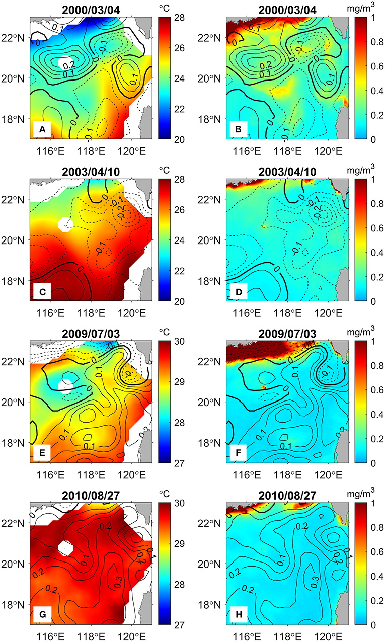
Figure 7. (Left) Spatial distribution of SST on March 4, 2000, April 10, 2003, July 3, 2009, and August 27, 2010. (Right) Same as the left-panel subfigures but are for the chlorophyll-a (Chl) distribution.

Figure 8 shows the particulate organic carbon fluxes obtained by in-situ observation and satellite estimation for the eddy cases in this study. Based on the satellite-derived POC fluxes, both AEs and CEs with significant eddy pumping (defined by the 10-m departure of D22 from the climatology) correspond to higher POC fluxes, compared with those with insignificant eddy pumping (20 ± 7 mg-C m⁻²day⁻¹). Specifically for the cases of AE2, AE3 and CE3 which have significant eddy pumping under the NE monsoon (December to May), the satellite-derived POC fluxes exceed 100 mg-C m⁻² day⁻¹ (Figure 8). The high POC flux could arise from a combination of eddy pumping and deepening of the wind-induced mixed layer (Zhou et al., 2020). In the core of AEs with significant downwelling, strong mixed-layer deepening could reach the nitracline (McGillicuddy, 2016), then increase Chl and POC fluxes near the surface. A positive correlation of Chl anomalies with the AEs could be found globally in nutrient-limited regions (McGillicuddy, 2016), such as the oligotrophic South Indian Ocean and subtropical Pacific (Gaube et al., 2014). Thus, we observed AEs with higher Chl and POC fluxes.

FIGURE 8

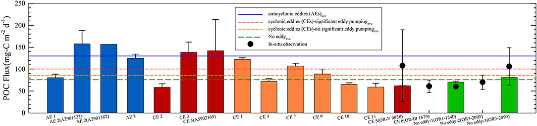
Figure 8. Particulate organic carbon (POC) fluxes for the eddy cases based on in situ observation (solid circles) and satellite estimation (color-shaded bars). The bars in blue, red, orange, and green show the POC fluxes corresponding to the cases with significant anticyclonic eddies (AEs) pumping, significant cyclonic eddies (CEs) pumping, insignificant CEs pumping, and no eddies, respectively. All error bars show the standard deviation of the POC fluxes. The horizontal solid and dashed lines show the total mean of POC flux for each case based on satellite estimation. We performed direct measurement of the POC flux given by Shih et al. (2020) for CE5 (OR-V 0038) and CE6 (OR-III 1679).

Based on the in-situ observation conducted in spring (March to May), the POC flux is higher near CE5 (May 2014) with significant upwelling than that near CE6 (April 2013) with insignificant upwelling. In addition, the CE5 POC flux was higher than that observed from the cruise experiment, OR-III 2093 (April 2019), which did not detect eddies in a similar region (Supplementary Figure S3D). The POC flux near CE5 was ~108 mg-C m⁻² day⁻¹ (Shih et al., 2020), the highest among the cruise experiments performed in this study, which were executed in the NSCS during spring. The estimation of POC fluxes near the eddy cores with significant eddy pumping in the NSCS was comparable with the high POC fluxes ranging from 83 to 194 mg-C m⁻²day⁻¹ observed around the eddies in the western North Pacific (Shih et al., 2015).

Overall, the particulate organic carbon (POC) fluxes are higher than 100 mg-C m⁻² day⁻¹ near the eddy cores with significant eddy pumping, but are smaller than 100 mg-C m⁻² day⁻¹ near the eddy cores with insignificant eddy pumping or regions with no detected eddies in the northern South China Sea (NSCS) (Figure 8). It is worth noting that the satellite-obtained POC fluxes may be underestimated when using the satellite-obtained Chl to calculate the NPP value in the NSCS (Li et al., 2018b). Based on three cruise experiments (Supplementary Figures S3B,C,E) with satellite POC-flux estimation, the difference between the satellite-obtained POC fluxes and the in-situ POC fluxes ranges from −42 to 17% (minus is for underestimated), showing the inconsistency of the satellite-estimated POC fluxes compared with the in situ-measured POC fluxes. The causes of these inconsistencies are complex, since the model-derived POC fluxes are based on three parameters, NPP, SST, and Z_eu that are obtained from the satellite data bank, suggesting more in situ-measured POC fluxes are needed to evaluate those model-derived values of POC fluxes in the NSCS.

Upper Ocean Stratification in the Eddy Cores

We hypothesized that when ocean stratification is weakened (smaller N²), eddy pumping is stronger according to the indirect estimation of vertical velocity (w) via the eddy pumping (McGillicuddy and Robinson, 1997; Sun et al., 2017):

$\begin{array}{ll}w=\frac{g}{{\rho }_0{N}^2}\left(\frac{\partial \rho }{\partial t}+u_r\frac{\partial \rho }{\partial r}+u_{\theta }\frac{1}{r}\frac{\partial \rho }{\partial \theta }\right)...& (8)\end{array}$

where t is the time, u_r and u_θ are the horizontal components of ocean currents in the r and θ direction, respectively, and other variables are the same as those in Equation (2). Besides the density evolution induced by the ocean eddies, the background N ² could also affect the amplitude of w. The smaller the N², the larger the amplitude of w. Moreover, water column stability was found to determine the formation of subtropical phytoplankton blooms in the northwestern Pacific (Matsumoto et al., 2021).

Figure 9 shows the anomaly profiles of squared buoyancy frequencies obtained via the expendable bathythermograph (XBT) transect that passed through the cyclonic eddies (CEs) and anticyclonic eddies (AEs). In Figures 9A,B, the anomaly profiles of squared buoyancy frequencies are mostly negative above 100 m around the cores of AE1 and CE8 with significant eddy pumping. To the west and east of these eddies, the squared buoyancy frequencies are lower than the climatological field above 100 m (Figures 9A,B), showing background weakening of upper ocean stratification. Averaged from the mixed layer depth at ~50 m to the thermocline bottom at ~162 m (Peng et al., 2018), the anomalies of squared buoyancy frequencies are −2 × 10⁻⁵ and −13 × 10⁻⁵ s⁻² around CE8 and AE1, respectively, in March 2000 and September 2008. For the eddies with insignificant vertical motion (Figures 9C,D), the anomalies of squared buoyancy frequencies are 4 × 10⁻⁵ and 8 × 10⁻⁵ s⁻² around AE4 and CE10, respectively, in September 2000 and July 2009. For the other two cases of CEs (CE9 and CE11) without significant upwelling observed in April 2003 and August 2010, the anomalies of squared buoyancy frequencies have a positive value, which is over 5 × 10⁻⁵ s⁻². This comparison suggests that weaker stratification from 50 to 162 m is the condition required for significant eddy vertical motion in the NSCS.

FIGURE 9

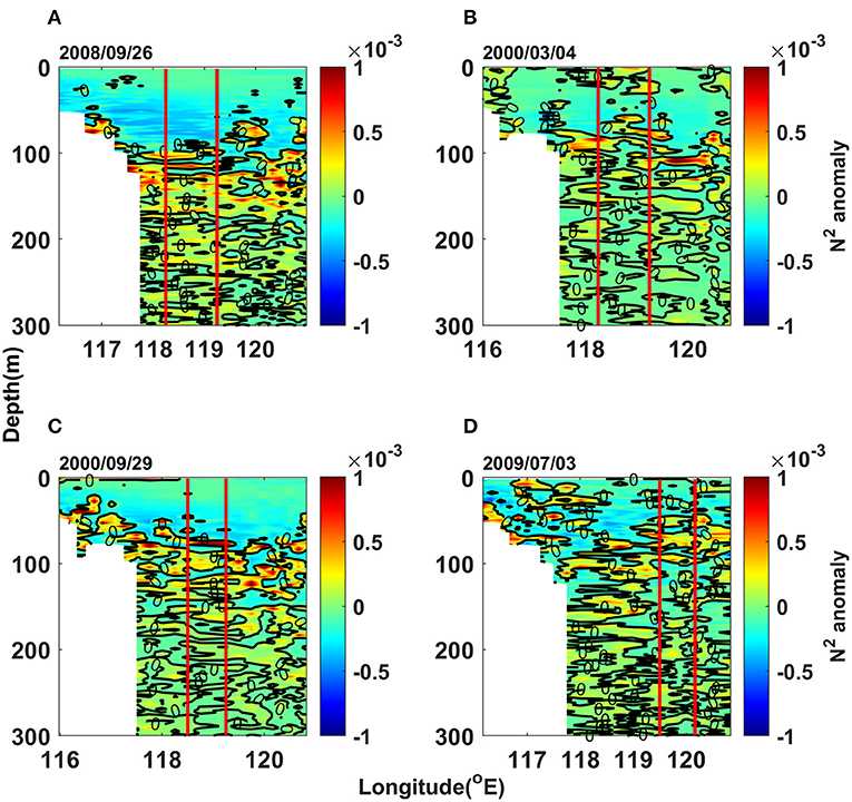
Figure 9. Anomalies of squared buoyancy frequency on (A) September 26, 2008 (AE1), (B) March 4, 2000 (CE8), (C) September 29, 2000 (AE4), and (D) July 3, 2009 (CE10), showing the background situation of ocean stratification around the eddies. The two red vertical lines show the region of eddies confirmed with satellite altimeters. The left (right) panel is for the cases of anticyclonic (cyclonic) eddies, while the upper (lower) panel is for the cases with (without) significant eddy pumping.

In addition to the expendable bathythermograph (XBT) observations, weaker stratification can also be found via the Argo floats that observed eddies with significant eddy pumping. Figure 3B shows a time series of N² anomaly profiles obtained from Argo 2900825 that observed the same anticyclonic eddy (AE1) that passed by the XBT transect in September 2008. Before and after observing AE1, the anomalies of N² are mostly negative above 100 m (Figure 3B), suggesting weaker stratification near the thermocline. Furthermore, to highlight the ocean background with weakened stratification at the Argo floats (Supplementary Table S1), Figure 10 represents the composite analysis of N² anomalies at the Argo locations during the months when the eddies were observed. The N² anomalies are generally negative around the depths from 50 and 162 m (around the thermocline depth) during the months when significant eddy pumping was observed near the core of AEs (Figure 10A) and CEs (Figure 10B). However, for the cases of CEs without significant upwelling, Figure 10B (gray curve) shows that the profiles of N² anomalies are positive around the depths from 50 to 162 m. This comparison suggests that ocean stratification is weaker than the climatological field from 50 to 162 m during the months when significant eddy pumping was observed in the NSCS.

FIGURE 10

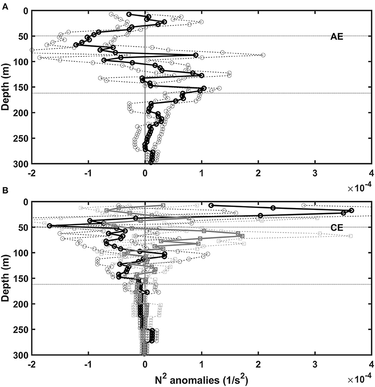
Figure 10. Mean (solid curve) and standard deviation (dashed curves) of N² anomalies at the location of Argo floats observing (A) four anticyclonic eddies with significant downwelling and (B) three cyclonic eddies with (black curve) and without (gray curve) significant upwelling.

Mechanism of Stratification Weakening

It is natural to ask what causes the stratification changes near the thermocline in the NSCS. We hypothesized that (1) the stratification is weakened when the lower ocean becomes lighter or the upper ocean becomes denser, and (2) the Kuroshio intrusion that brings lighter surface waters via the Luzon Strait strengthens the ocean stratification, which tends to suppress eddy pumping. To prove these hypotheses, Figure 11 shows the background temperature changes in ocean vertical profiles in the SCS during the month and a month before the observation of the ocean eddies. Compared with the climatological fields below 100 m, the water is warmer and lighter in the NSCS but is colder and denser in the SSCS for both AEs (Figures 11A,B) and CEs (Figures 11C,D) with significant eddy pumping. However, for the eddy cases without significant eddy pumping (Figures 11E,F), the water is warmer and lighter from 50 to 100 m in the whole SCS. This comparison suggests that when the NSCS is lighter and warmer below the thermocline, the stratification near the thermocline becomes weak and forms a background condition favorable for significant eddy pumping to occur near eddy cores.

FIGURE 11

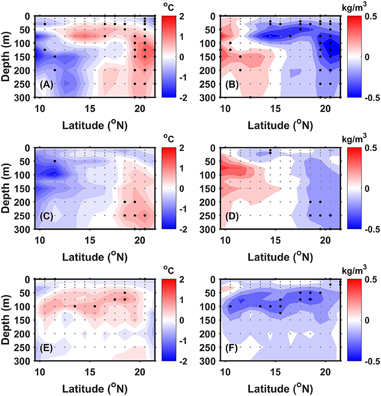
Figure 11. Meridional distribution of the anomalies in temperature (left) and potential density (right) averaged within 108°E and 121°E during the month and a month before observing the ocean eddies, using the temperature-salinity (TS) gridded data of World Ocean Database version 13 (WOD13). (A,B) For the anticyclonic eddies with significant downwelling. (C,D) For the cyclonic eddies with significant upwelling. (E,F) For all the eddies without significant upwelling or downwelling. The gray dots show the data points to plot the contours, and the black dots shows the data points significant to the 95% confidence level based on t-testing. Note that the statistical analysis in (E,F) does not include the case of Argo 2902045 in May 2017 because of the data availability of TS gridded data of WOD13 up to 2014.

To examine the causes of warming in the northern South China Sea (NSCS), Figure 12 shows the TS properties of seawater obtained from the Argo floats that observed significant eddy pumping, compared with the background TS in the SSCS (east of Vietnam coast) and the region east of Luzon island (for the Kuroshio). In Figure 12A, the TS properties, which were observed via Argo 2900825 in the NSCS between August and September 2008, are occasionally similar to those observed in the SSCS. TS properties similar to those of the SSCS can be found in the other cases with significant downwelling (Figure 12, left) and upwelling (Figure 12, right). These TS diagrams suggest that the warm water in the NSCS comes from the SSCS.

FIGURE 12

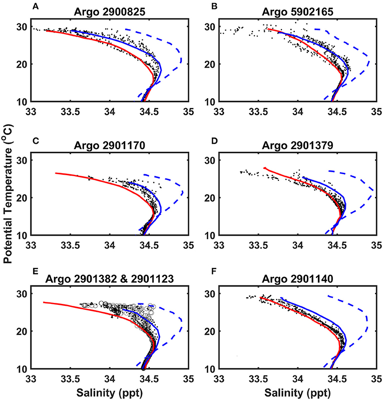
Figure 12. Temperature-salinity (TS) diagrams during the month and a month before observing the ocean eddies via Argos (A) 2900825, (B) 5902165, (C) 2901170, (D) 2901379, (E) 2901382, 2901123, and (F) 2901140. The left and right panels are for anticyclonic and cyclonic eddies, respectively. The solid red and dashed blue curve represents the TS properties of water masses in the southern South China Sea (SCS) and in the Kuroshio region, respectively. In (E), the dots are for the TS obtained from Argo 2901123 and the circles are for Argo 2901382, observing the same anticyclonic eddy with significant downwelling.

To show the northward transport of South China Sea (SCS) water, Figure 13 shows the Sverdrup transports in the SCS averaged within 109°E and 120°E during the month and a month before observing the eddies via the Argo floats and XBTs. As shown in Figure 13A, the Sverdrup transports are mostly positive (northward) south of 18°N for all the cases with significant eddy pumping. In contrast, Figure 13B shows that most cases with insignificant eddy pumping (except AE4, CE10, and CE11) are accompanied by negative (southward) or small positive Sverdrup transports south of 17°N. Within 12°N and 22°N, the net Sverdrup transports for cases with significant eddy pumping range from 0.7 to 2.6 Sv, larger than those with insignificant eddy pumping (−0.4 to 1.8 Sv). This comparison suggests that the wind-induced Sverdrup transports bring the SSCS water northward into the NSCS during the month and a month before observing the ocean eddies with significant eddy pumping.

FIGURE 13

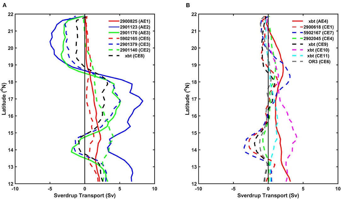
Figure 13. Meridional distribution of Sverdrup transport averaged within 109°E and 120°E during the month and a month before observing the ocean eddies via Argo floats and expendable bathythermographs (XBTs). (A) Cases with significant eddy pumping. (B) Cases without significant eddy pumping. Solid and dashed curves are for the anticyclonic and cyclonic eddies, respectively. Only considering depth larger than 100 m.

Even with the positive Sverdrup transports, the eddy pumping of AE4, CE10, and CE11 was insignificant along the XBT transects near the Luzon Strait in September 2000, July 2009, and August 2010, respectively. To determine why this is the case, we searched for all the available historical data of ocean profiles from Argo and CTD observations. Fortunately, Argo 2901180 was close to the XBT transect on July 8, 2009 (Supplementary Figure S3F), 5 days after the CE10 core was observed via the XBTs. Besides, CTD casting was found near the XBT transect on September 17, 2000 and August 16, 2010, about 10 days before the core of AE4 and CE11, respectively, were observed (Supplementary Figure S3F). Based on these ocean profiles, Figure 14 shows that warmer and more saline water coming from the Kuroshio can be found near the XBT transect, showing the Kuroshio intrusion into the Luzon Strait at the time the eddy cores without significant eddy pumping were observed. The Kuroshio intrusion causes lighter water in the upper layer enhancing the ocean stratification near the thermocline; thus, it may depress the eddy pumping of AE4, CE10, and CE11 even though the Sverdrup transports are positive in the SCS.

FIGURE 14

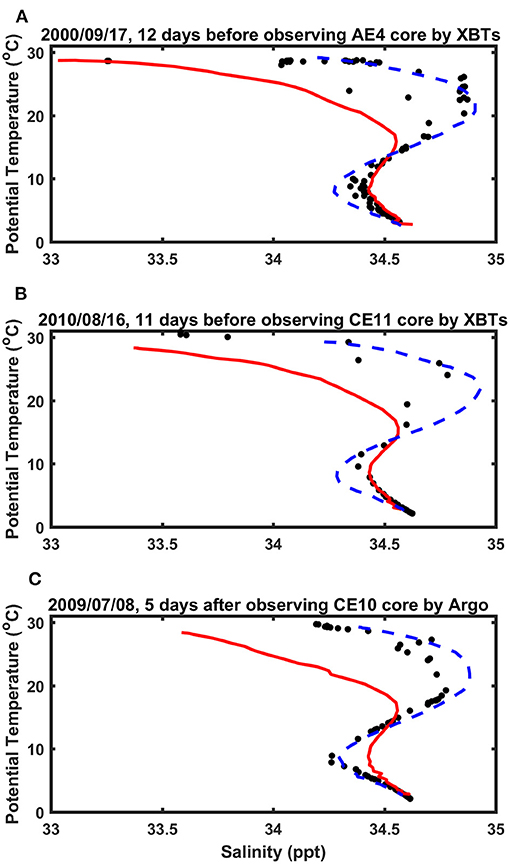
Figure 14. Temperature-salinity (TS) diagrams corresponding to the cases with insignificant eddy pumping and the positive Sverdrup transport, on a particular date closest to day when observing the eddy core via expendable bathythermographs (XBTs). The TS data obtained from (A) the ODB-CTD data for September 17, 2000, (B) the ODB-CTD data for August 16, 2010, and (C) the Argo 2901180 data for July 8, 2009. The solid red and dashed blue curve represents the TS properties of water masses in the southern South China Sea (SCS) and in the Kuroshio region, respectively.

Summary

In general, cyclonic eddies and anticyclonic eddies can be accompanied by upwelling and downwelling, respectively, near the eddy core. However, we observed eddies with and without significant eddy pumping via a repeated XBT transect, Argo floats, and cruise experiments in the NSCS.

By studying the ocean vertical structure case by case from 2000 to 2017, eddies with and without significant pumping were found in different monsoons. The analysis showed that the ocean stratification near the thermocline was an important factor in determining eddy pumping in the NSCS. When the ocean stratification was weaker than the climatological field, significant upwelling (downwelling) was observed near the cores of CEs (AEs), although the eddies could only be traced back for 10 days. However, in the same trace-back period, some eddies had no significant upwelling and downwelling near their cores when the ocean stratification was stronger than the climatological field. When waters were transported northward into the NSCS, the thermocline became weaker because of decreasing density vertical gradients (the weakening of the ocean stratification) caused by the lighter and warmer waters transported from the SSCS. Under such conditions with thermocline weakening, significant upwelling and downwelling were observed near the cores of CEs and AEs, respectively.

The biogeochemical response to significant upwelling near a cyclonic eddy (CE5) was observed via a cruise experiment executed in May 2014, although the cyclonic eddy (CE5) had a small diameter (50 to 100 km), compared with the mean radius of eddies in the SCS. A higher concentration of nutrients was found near the core of the cyclonic eddy (CE5) where the upwelling occurred. With an increasing concentration of N near the eddy core, the N:P ratio became larger than 16:1 (the Redfield ratio) at some depths above the thermocline, in contrast to the marine environment in the background NSCS. The POC flux was higher than 100 mg-Cm⁻² day⁻¹ near the eddy cores with significant eddy pumping, obtained by in situ measurement and satellite estimation. although the satellite-estimated POC fluxes were inconsistent compared with the measured POC fluxes.

Data Availability Statement

The raw data supporting the conclusions of this article will be made available by the authors, without undue reservation, to any qualified researcher.

Author Contributions

C-CH and CC wrote the manuscript. Y-YS executed the experiments and collected water samples for the biogeochemical part of this study. CC and Y-TC detected eddies and studied ocean vertical structure. JC and NF analyzed the nutrient samples and provided Figures 7, 9. W-CW analyzed satellite images and provided Figure 8. CC, Y-YS, and C-CH revised the manuscript. All authors contributed to the article and approved the submitted version.

Funding

This study is supported by the Ministry of Science and Technology (MOST), Taiwan (ROC), under the project Eddy roles in marine environmental variability near Taiwan (105-2119-M-110-011-MY2, 105-2119-M-019-009-MY2, 107-2611-M-019-020-MY2, and 109-2611-M-019-013), I-Taiwan grants from MOST (107-2611-M-019-020-MY2, 108-2611M-110-019-MY3, 108-2917-I-564-017, and 109-2611-M-019-013) and Influences of typhoons and internal waves on in situ and remote carbon fixation of phytoplankton in the northern South China Sea (II)(III) (109-2611-M-012-001 and 110-2611-M-012-002).

Conflict of Interest

The authors declare that the research was conducted in the absence of any commercial or financial relationships that could be construed as a potential conflict of interest.

Publisher's Note

All claims expressed in this article are solely those of the authors and do not necessarily represent those of their affiliated organizations, or those of the publisher, the editors and the reviewers. Any product that may be evaluated in this article, or claim that may be made by its manufacturer, is not guaranteed or endorsed by the publisher.

Acknowledgments

We thank the Coriolis Operational Oceanography (http://www.coriolis.eu.org), NOAA, and Taiwan ODB for providing the data of ocean profiles based on the Argo floats, XBTs, CTD, WOD13, and WOA13. We also thank CMEMS and RSS (https://www.remss.com/) for the satellite data of SLAs, ocean color, and SST. We are grateful to the captains and crews of the R/Vs OR-I, OR-III, and OR-V for their efforts in executing the sea-going experiments in the NSCS.

Supplementary Material

The Supplementary Material for this article can be found online at: https://www.frontiersin.org/articles/10.3389/fmars.2021.717576/full#supplementary-material

References

Behrenfeld, M. J., and Falkowski, P. G. (1997). Photosynthetic rates derived from satellite-based chlorophyll concentration. Limnol. Oceanogr. 42, 1–20. doi: 10.4319/lo.1997.42.1.0001

CrossRef Full Text | Google Scholar

Chelton, D. B., Gaube, P., Schlax, M. G., Early, J. J., and Samelson, R. M. (2011a). The influence of nonlinear mesoscale eddies on near-surface oceanic chlorophyll. Science 334, 328–332. doi: 10.1126/science.1208897

PubMed Abstract | CrossRef Full Text | Google Scholar

Chelton, D. B., Schlax, M. G., and Samelson, R. M. (2011b). Global observations of nonlinear mesoscale eddies. Prog. Oceanogr. 91. 167–216. doi: 10.1016/j.pocean.2011.01.002

CrossRef Full Text | Google Scholar

Chen, C. C., Shiah, F. K., Chung, S. W., and Liu, K. K. (2006). Winter phytoplankton blooms in the shallow mixed layer of the South China Sea enhanced by upwelling. J. Mar. Syst. 59, 97–110. doi: 10.1016/j.jmarsys.2005.09.002

CrossRef Full Text | Google Scholar

Chen, G., and Han, G. (2019). Contrasting short-lived with long-lived mesoscale eddies in the global ocean. J. Geophys. Res. Oceans. 124, 3149–3167. doi: 10.1029/2019JC014983

CrossRef Full Text | Google Scholar

Chen, G., Hou, Y., and Chu, X. (2011). Mesoscale eddies in the South China Sea: mean properties, spatiotemporal variability, and impact on thermohaline structure. J. Geophys. Res. 116, C06018. doi: 10.1029/2010JC006716

CrossRef Full Text | Google Scholar

Chen, K. S., Hung, C. C., Gong, G. C., Chou, W. C., Chung, C. C., and Shih, Y. Y. (2013). Enhanced POC export in the oligotrophic northwest Pacific Oceanafter extreme weather events. Geophys. Res. Lett. 40, 5728–5734. doi: 10.1002/2013GL058300

CrossRef Full Text | Google Scholar

Chen, Y. L., Chen, H. Y., Lin, I. I, Lee, M. A, and Chang, J. (2007). Effects of cold eddy on phytoplankton production and assemblages in LuzonStrait bordering the South China Sea. J. Oceanogr. 63, 671–683. doi: 10.1007/s10872-007-0059-9

CrossRef Full Text | Google Scholar

Chen, Y. L. L. (2005). Spatial and seasonal variations of nitrate-based new production and primary production in the South China Sea. Deep-Sea Res. I. 52, 319–340. doi: 10.1016/j.dsr.2004.11.001

CrossRef Full Text | Google Scholar

Chen, Y. L. L., Chen, H. Y., Jan, S., Lin, Y. H., Kuo, T. H., and Hung, J. J. (2015), Biologically active warm-core anticyclonic eddies in the marginal seas of the western pacific ocean. Deep Sea Res. Part I Oceanogr. Res. Pap. 106, 68–84. doi: 10.1016/j.dsr.2015.10.006

CrossRef Full Text | Google Scholar

Chen, Y. L. L., Chen, H. Y., Karl, D. M, and Takahashi, M (2004). Nitrogen modulates phytoplankton growth in spring in the South China Sea. Cont. Shelf Res. 24, 527–541. doi: 10.1016/j.csr.2003.12.006

CrossRef Full Text | Google Scholar

Chow, C.-H., Hu, J.-H., Centurioni, L. R., and Niiler, P. P. (2008). Mesoscale Dongsha cyclonic Eddy in the northern South China Sea by drifter and satellite observations. J. Geophys. Res. 113:C04018. doi: 10.1029/2007JC004542

CrossRef Full Text | Google Scholar

Chow, C. H., Cheah, W., and Tai, J.-H. (2017). A rare and extensive summer bloom enhanced by ocean eddies in the oligotrophic western North Pacific Subtropical Gyre. Sci. Rep. 7:6199. doi: 10.1038/s41598-017-06584-3

PubMed Abstract | CrossRef Full Text | Google Scholar

Chow, C. H., Cheah, W., Tai, J.-H., and Liu, S.-F. (2019). Anomalous wind triggered the largest phytoplankton bloom in the oligotrophic North Pacific Subtropical Gyre. Sci. Rep. 9:15550. doi: 10.1038/s41598-019-51989-x

PubMed Abstract | CrossRef Full Text | Google Scholar

Chow, C. H., Liu, Q., and Xie, S.-P. (2015). Effects of Kuroshio Intrusions on the atmosphere northeast of Taiwan Island. Geophys. Res. Lett. 42, 1465–1470. doi: 10.1002/2014GL062796

CrossRef Full Text | Google Scholar

Chu, P. C., and Fan, C. W. (2017). Synoptic monthly gridded global and regional four dimensional WOD and GTSPP (T, S, u, v) fields with the optimal spectral decomposition (OSD) and P-vector methods. Geosci. Data J. 4, 50–71. doi: 10.1002/gdj3.48

CrossRef Full Text | Google Scholar

Chu, X., Chen, G., and Qi, Y. (2020). Periodic mesoscale Eddies in the South China Sea. J. Geophys. Res. Oceans. 125:e2019JC015139. doi: 10.1029/2019JC015139

CrossRef Full Text

Du, Y., Wu, D., Liang, F., Yi, J., Mo, Y., He, Z., et al. (2016). Major migration Corridors of Mesoscale Ocean Eddies in the South China Sea from 1992 to 2012. J. Mar. Syst. 158, 173–181. doi: 10.1016/j.jmarsys.2016.01.013

CrossRef Full Text | Google Scholar

Dunne, J. P., Armstrong, R. A., Gnanadesikan, A., and Sarmiento, J. L. (2005). Empirical and mechanistic models for the particle export ratio. Global Biogeochem. Cy. 19:GB4026. doi: 10.1029/2004GB002390

CrossRef Full Text | Google Scholar

Faghmous, J. H., Frenger, I., Yao, Y., Warmka, R., Lindell, A., and Kumar, V. (2015). A daily global mesoscale ocean eddy dataset from satellite altimetry. Sci. Data. 2:150028. doi: 10.1038/sdata.2015.28

PubMed Abstract | CrossRef Full Text | Google Scholar

Flagg, C. N., Wallace, D., and Kolber, Z. (1998). Cold anti-cyclonic eddies formed from cold pool water in the southernmiddle Atlantic bight. Cont. Shelf Res. 15, 1839–1867. doi: 10.1016/S0278-4343(97)00038-1

CrossRef Full Text | Google Scholar

Gaube, P., McGillicuddy Jr, D. J., Chelton, D. B., Behrenfeld, M. J., and Strutton, P. G. (2014). Regional variations in the influence of mesoscale eddies on near-surface chlorophyll. J. Geophys. Res. Oceans 119, 8195–8220, doi: 10.1002/2014JC010111

CrossRef Full Text | Google Scholar

Gill, A. (1982), Atmosphere–Ocean Dynamics. New York, NY: Academic Press.

Google Scholar

Hu, J. Y., Kawamura, H., Hong, H. S., and Qi, Y. Q. (2000). A review on the currents in the South China Sea: seasonal circulation, South China Sea warm current and Kuroshio intrusion. J. Oceanogr. 56, 607–624. doi: 10.1023/A:1011117531252

CrossRef Full Text | Google Scholar

Huang, J., and Xu, F. (2018). Observational evidence of subsurface chlorophyll response to mesoscale eddies in the North Pacific. Geophys. Res. Lett. 45, 8462–8470. doi: 10.1029/2018GL078408

CrossRef Full Text | Google Scholar

Hung, C.-C., Gong, G.-C., Chou, W.-C., Chung, C.-C., Lee, M.-A., and Chang, Y. (2010b). The effect of typhoon on particulateorganic carbon flux in the southern East China Sea. Biogeosciences 7, 3521–3550. doi: 10.5194/bg-7-3007-2010

CrossRef Full Text | Google Scholar

Hung, C.-C., Gong, G.-C., Chung, W.-C., Kuo, W.-T., and Lin, F.-C. (2009). Enhancement of particulate organic carbon export flux induced by atmospheric forcing in the subtropical oligotrophic northwest Pacific Ocean. Mar. Chem. 113, 19–24 doi: 10.1016/j.marchem.2008.11.004

CrossRef Full Text | Google Scholar

Hung, C.-C., Guo, L., Schultz Jr, G. E., Pinckney, J. L., and Santschi, P. H. (2003). Production and flux of carbohydrate species inthe Gulf of Mexico. Global Biogeochem. Cy. 17:1055. doi: 10.1029/2002GB001988

CrossRef Full Text | Google Scholar

Hung, C.-C., Xu, C., Santschi, P. H., Zhang, S.-J., Schwehr, K. A., Quigg, A., et al. (2010a). Comparative evaluation of sediment trap and ²³⁴Th-derived POC fluxes from the upper oligotrophic waters of the Gulf of Mexico and the subtropical northwestern Pacific Ocean. Mar. Chem. 121, 132–144. doi: 10.1016/j.marchem.2010.03.011

CrossRef Full Text | Google Scholar

Hwang, C., and Chen, S. A. (2000). Circulations and eddies over the South China Sea derived from TOPEX/Poseidon altimetry. J. Geophys. Res. 105, 23943–23965. doi: 10.1029/2000JC900092

CrossRef Full Text | Google Scholar

Itoh, S., and Yasuda, I. (2010). Water mass structure of warm and cold anticyclonic eddies in the western boundary region of the Subarctic North Pacific. J. Phys. Oceanogr. 40, 2624–2642. doi: 10.1175/2010JPO4475.1

CrossRef Full Text | Google Scholar

Kudo, I. (2003). Change in the uptake and cellular Si:N ratio in diatoms responding to the ambient Si:N ratio and growth phase. Mar. Biol. 143, 39–46. doi: 10.1007/s00227-003-1063-2

CrossRef Full Text | Google Scholar

Large, W. G., and Pond, S. (1982). Sensible and latent heat flux measurements over the ocean. J. Phys. Oceanogr. 12, 464–482. doi: 10.1175/1520-0485(1982)012andlt;0464:SALHFMandgt;2.0.CO;2

CrossRef Full Text | Google Scholar

Li, D., Chou, W.-C., Shih, Y.-Y., Chen, G.-Y., Chang, Y., Chow, C. H., et al. (2018a). Elevated particulate organic carbon export flux induced by internal waves in the oligotrophic northern South China Sea. Sci. Rep. 8:2042. doi: 10.1038/s41598-018-20184-9

PubMed Abstract | CrossRef Full Text | Google Scholar

Li, L., Worth, D. N., and Su, J. (1998). Anticyclonic rings from the Kuroshio in the South China Sea. Deep Sea Res. Part I. 45, 1469–1482. doi: 10.1016/S0967-0637(98)00026-0

CrossRef Full Text | Google Scholar

Li, T., Bai, Y., He, X., Xie, Y., Chen, X., Gong, F., et al. (2018b). Satellite-based estimation of particulate organic carbon export in the northern South China Sea. J. Geophys. Res. Oceans. 123, 8227–8246. doi: 10.1029/2018JC014201

CrossRef Full Text | Google Scholar

Liu, K. K., Chao, S. Y., Shaw, P. T., Gong, G. C., Chen, C. C., and Tang, T. Y. (2002). Monsoon-forced chlorophyll distribution and primary production in the South China Sea: observations and a numerical study. Deep Sea Res. I. 49, 1387–1412. doi: 10.1016/S0967-0637(02)00035-3

CrossRef Full Text | Google Scholar

Liu, Y., Yu, L., and Chen, G. (2020). Characterization of sea surface temperature and air-sea heat flux anomalies associated with mesoscale eddies in the South China Sea. J. Geophys. Res. Oceans 125:e2019JC015470. doi: 10.1029/2019JC015470

CrossRef Full Text | Google Scholar

Ma, W., Xiu, P., Chai, F., Ran, L., Wiesner, M. G., Xi, J., et al. (2021). Impact of mesoscale eddies on the source funnel of sediment trap measurements in the South China Sea. Prog. Oceanogr. 194:102566. doi: 10.1016/j.pocean.2021.102566

CrossRef Full Text | Google Scholar

Matsumoto, K., Sasai, Y., Sasaoka, K., Siswanto, E., and Honda, M. C. (2021). The formation of subtropical phytoplankton blooms is dictated by water column stability during winter and spring in the oligotrophic northwestern North Pacific. J. Geophys. Res. Oceans 126:e2020JC016864. doi: 10.1029/2020JC016864

CrossRef Full Text | Google Scholar

McGillicuddy, D. J. (2016), Mechanisms of physical-biological-biogeochemical interaction at the oceanic mesoscale. Ann. Rev. Mar. Sci. 8, 125–159. doi: 10.1146/annurev-marine-010814-015606.

PubMed Abstract | CrossRef Full Text | Google Scholar

McGillicuddy, D. J., and Robinson, A. R. (1997). Eddy-induced nutrient supply and new production in the Sargasso Sea. Deep Sea Res. Part I 44, 1427–1450. doi: 10.1016/S0967-0637(97)00024-1

CrossRef Full Text | Google Scholar

Nan, F., Xue, H. J., and Yu, F. (2015). Kuroshio intrusion into the South China Sea: a review. Prog. Oceanogr. 137, 314–333. doi: 10.1016/j.pocean.2014.05.012

CrossRef Full Text | Google Scholar

Okubo, A. (1970). Horizontal dispersion of floatable particles in the vicinity of velocity singularities such as convergences. Deep Sea Res. Oceanogr. Abstr. 17, 445–454. doi: 10.1016/0011-7471(70)90059-8

CrossRef Full Text | Google Scholar

Peng, H., Pan, A., Zheng, Q. A., and Hu, J. (2018). Analysis of monthly variability of thermocline in the South China Sea. J. Oceanol. Limnol. 36, 205–215. doi: 10.1007/s00343-017-6151-0

CrossRef Full Text | Google Scholar

Shen, S., Leptoukh, G. G., Acker, J. G., Yu, Z., and Kempler, S. (2008). Seasonal variations of chlorophyll a concentration in the Northern South China Sea. IEEE Geosci. Remote Sens. Lett. 5, 315–319. doi: 10.1109/LGRS.2008.915932

CrossRef Full Text | Google Scholar

Shih, Y.-Y., Hung, C.-C., Gong, G.-C., Chung, W. C., Wang, Y.-H., Lee, I.-H., et al. (2015). Enhanced particulate organic carbon export at Eddy edges in the oligotrophic Western North Pacific Ocean. PLoS ONE 10:e0131538. doi: 10.1371/journal.pone.0131538

PubMed Abstract | CrossRef Full Text | Google Scholar

Shih, Y.-Y., Hung, C.-C., Huang, S.-Y., Muller, F. L. L., and Chen, Y.-H. (2020). Biogeochemical variability of the upper ocean response to typhoons and storms in the northern South China Sea. Front. Mar. Sci. 7:151. doi: 10.3389/fmars.2020.00151

CrossRef Full Text | Google Scholar

Shih, Y.-Y., Lin, H.-H., Li, D., Hsieh, H.-H., Hung, C.-C., and Chen, C.-T. A. (2019). Elevated carbon flux in deep waters of the South China Sea. Sci. Rep. 9:1496. doi: 10.1038/s41598-018-37726-w

PubMed Abstract | CrossRef Full Text | Google Scholar

Shih, Y. Y., Hsieh, J. S., Gong, G. C., Chou, W. C., Lee, M. A., Hung, C. C., et al. (2013). Field observations of changes in SST, chlorophyll and POC flux in the southern East China Sea before and after the passage of typhoon Jangmi. Terr. Atmos. Ocean. Sci. 24, 899–910. doi: 10.3319/TAO.2013.05.23.01(Oc)

CrossRef Full Text | Google Scholar

Siegel, D. A., Peterson, P., McGillicuddy, D. J., Maritorena, S., and Nelson, N. B. (2011). Bio-optical footprints created by mesoscale eddies in the Sargasso Sea. Geophys. Res. Lett. 38:L13608. doi: 10.1029/2011GL047660

CrossRef Full Text | Google Scholar

Siswanto, E., Ishizaka, J., Morimoto, A., Tanaka, K., Okamura, K., and Kristijono, A. (2008). Ocean physical and biogeochemical responses to the passage of Typhoon Meari in the East ChinaSea observed from Argo float and multiplatform satellites. Geophys. Res. Lett. 35:L15604. doi: 10.1029/2008GL035040

CrossRef Full Text | Google Scholar

Siswanto, E., Ishizaka, J., Yokouchi, K., Tanaka, K., and Tan, C. K. (2007). Estimation of interannual andinterdecadal variations of typhoon-induced primary production: a cases study for the outer shelfof the East China Sea. Geophys. Res. Lett. 34:L03604. doi: 10.1029/2006GL028368

CrossRef Full Text | Google Scholar

Soong, Y. S., Hu, J. H., Ho, C. R., and Niiler, P. P. (1995). Cold cool eddy detected in South China Sea. Eos Trans. AGU. 76, 345–347. doi: 10.1029/95EO00209

CrossRef Full Text | Google Scholar

Su, J. (2004). Overview of the South China Sea circulation and its influence on the coastal physical oceanography outside the Pearl River Estuary. Cont. Shelf Res. 24, 1745–1760. doi: 10.1016/j.csr.2004.06.005

CrossRef Full Text | Google Scholar

Sun, W., Dong, C., Tan, W., and He, Y. (2019). Statistical characteristics of cyclonic warm-core eddies and anticyclonic cold-core eddies in the North Pacific based on remote sensing data. Remote Sens. 11:208. doi: 10.3390/rs11020208

CrossRef Full Text | Google Scholar

Sun, W., Dong, C., Tan, W., Liu, Y., He, Y., and Wang, J. (2018), Vertical structure anomalies of oceanic Eddies Eddy-induced transports in the South China Sea. Remote Sens. 10:795. doi: 10.3390/rs10050795

CrossRef Full Text | Google Scholar

Sun, W., Dong, C., Wang, R., Liu, Y., and Yu, K. (2017). Vertical structureanomalies of oceanic eddies in the Kuroshio Extension region. J. Geophys. Res. Oceans 122, 1476–1496. doi: 10.1002/2016JC012226

CrossRef Full Text | Google Scholar

Tai, J. H., Chou, W. C., Hung, C. C., Wu, K. C., Chen, Y. H., Chen, T. Y., et al. (2020). Short-term variability of biological production and CO₂ system around dongsha atoll of the Northern South China sea: impact of topography-flow interaction. Front. Mar. Sci. 7:511. doi: 10.3389/fmars.2020.00511

CrossRef Full Text | Google Scholar

Vignudelli, S., Cipollini, P., Reseghetti, F., Fusco, G., Gasparini, G. P., and Manzella, G. M. R. (2003). Comparison between XBT data and TOPEX/Poseidon satellite altimetry in the Ligurian-Tyrrhenian area. Ann. Geophys. 21, 123–135. doi: 10.5194/angeo-21-123-2003

CrossRef Full Text | Google Scholar

Wang, G. H., Su, J. L., and Chu, P. C. (2003). Mesoscale eddies in the South China Sea observed with altimeter data. Geophys. Res. Lett. 30:2121. doi: 10.1029/2003GL018532

CrossRef Full Text | Google Scholar

Weiss, J. (1991). The dynamics of enstrophy transfer in 2-dimensional hydrodynamics. Phys. D. 48, 273–294. doi: 10.1016/0167-2789(91)90088-Q

CrossRef Full Text | Google Scholar

Wu, J., Chung, S.-W., Wen, L.-S., Liu, K.-K., Chen, Y.-L. L., Chen, H.-Y., et al. (2003). Dissolved inorganic phosphorus, dissolved iron, and Trichodesmium in the oligotrophic South China Sea. Global Biogeochem. Cy. 17:1008. doi: 10.1029/2002GB001924

CrossRef Full Text | Google Scholar

Wu, W., Huang, B., and Zhong, C. (2014). Photosynthetic picoeukaryote assemblages in the South China Sea from the Pearl River estuary to the SEATS station. Aqua. Microb. Ecol. 71, 271–284. doi: 10.3354/ame01681

CrossRef Full Text | Google Scholar

Xiu, P., and Chai, F. (2011). Modeled biogeochemical responses to mesoscale eddies in the South China Sea. J. Geophys. Res. 116:C10006. doi: 10.1029/2010JC006800

CrossRef Full Text | Google Scholar

Xiu, P., Chai, F., Shi, L., Xue, H., and Chao, Y. (2010). A census of eddy activities in the South China Sea during 1993–2007. J. Geophys. Res. 115:C03012. doi: 10.1029/2009JC005657

CrossRef Full Text | Google Scholar

Zhang, W.-Z., Wang, H., Chai, F., and Qiu, G. (2016). Physical drivers of chlorophyll variability in the open South China Sea. J. Geophys. Res. Oceans 121, 7123–7140. doi: 10.1002/2016JC011983

CrossRef Full Text | Google Scholar

Zhang, Z., Qiu, B., Klein, P., and Travis, S. (2019). The influence of geostrophic strain on oceanic ageostrophic motion and surface chlorophyll. Nat. Commun. 10:2838. doi: 10.1038/s41467-019-10883-w

PubMed Abstract | CrossRef Full Text | Google Scholar

Zhou, K., Dai, M., Maiti, K., Chen, W., Chen, J., Hong, Q., et al. (2020). Impact of physical and biogeochemical forcing on particle export in the South China Sea. Prog. Oceanogr. 187:102403. doi: 10.1016/j.pocean.2020.102403

CrossRef Full Text | Google Scholar