Poleward Propagation of Typhoon-Induced Near-Inertial Waves in the Northern South China Sea

One of the main responses of the ocean to typhoons is the generation of near-inertial waves (NIWs), whose intrinsic frequency is close to the local inertial frequency. Based on the mooring observations, we carefully investigated the spatial–temporal variations in NIWs in the northern South China Sea (SCS) after Typhoon “Haima,” which passed through the northern SCS from October 20 to 21, 2016, with its track parallel to the mooring array on its northeast side. Moorings in different locations responded differently to this typhoon, with stronger NIWs found on the continental slope to the shelf break and relatively weak NIWs found on the shallow continental shelf. Strong NIWs appeared twice within a short period and showed different characteristics and frequencies. The first NIWs were generated locally with blue-shifted (super-inertial) frequencies. These initial NIWs were dominated by the first three baroclinic modes and rapidly weakened due to their propagation away and local dissipation. However, the second NIWs mainly consisted of higher baroclinic modes with red-shifted (sub-inertial) frequencies. The analysis of the mean background flow revealed that these red-shifted NIWs were excited at low latitudes, and subsequently advected by the poleward background flow to moorings whose latitudes were higher than their critical latitudes. Higher-mode (n > 3) NIWs were more easily carried away by mean background flow, and, at the same time, high-mode NIWs propagated downward to the subsurface layer, leading to the significant elevation of velocity shear therein. Given these findings, the mean background flow may provide an important route to redistributing the energy of the upper ocean imported from typhoons.

Introduction

In traditional internal wave theory, the internal gravity waves with an intrinsic frequency close to the local inertial frequency f (f = 2Ωsinθ; Ω is the angular velocity of the Earth and θ is the latitude (Gill, 1982)) are usually referred to as near-inertial internal waves (NIWs). The NIWs exist everywhere in the ocean except at the equator (Jeon et al., 2019). When wind with a high spatiotemporal variation acts on the upper ocean, it will generate a flow with a near-inertial period (Maeda et al., 1996; Guan et al., 2014). Therefore, one of the main dynamic responses of the ocean to tropical cyclones is the generation of NIWs (Price et al., 1994; Garrett, 2003; Yang and Hou, 2014).

The South China Sea (SCS) is not only an area frequently traversed by tropical cyclones from the northwestern Pacific Ocean but also the birthplace of local tropical cyclones. Therefore, many studies have focused on the NIWs induced by tropical cyclones in this area. The NIWs induced by tropical cyclones are often dominated by upward phase propagation and corresponding downward energy propagation. The energy will mainly be distributed from the bottom of the mixed layer to the upper thermocline and will decay rapidly in several inertial cycles (Chen, 2007; Sun et al., 2012; Guan et al., 2014). The characteristics (e.g., wave amplitude, duration, phase propagation, and frequency shift) of these NIWs are largely modulated by the wind field and background ocean conditions (Sun et al., 2015; Alford et al., 2016). The properties of typhoon forcing, such as trajectory, wind speed, translation speed, radius of maximum wind, and distance to the observation site, constitute the key parameters determining the resultant NIWs (Cao et al., 2018; Xu et al., 2019). In addition, the ocean conditions, such as mesoscale eddies (Oey et al., 2008; Chen et al., 2013; Fer et al., 2018), ocean fronts (Rubino et al., 2010; Alford et al., 2013), and background flows (Kunze, 1985; Xie et al., 2015; Jeon et al., 2019) play an important role in shaping the NIWs induced by typhoons. In the SCS, the background flow can undergo significant variability due to the alternating monsoon, complex topography, and changeable hydrologic structure. Therefore, the characteristics of NIWs in this area can be much more complicated (Boyer et al., 2020).

Among these complex features, one of the most striking features is the frequency shift. The frequencies of NIWs induced by tropical cyclones are usually shifted 1–20% above the local inertial frequency (Alford et al., 2016), which is called as “blue-shift.” After generation, the distribution of NIWs is traditionally thought to be governed by equatorward propagation (D'Asaro, 1985; Alford, 2001; Alford and Gregg, 2001), meaning that NIWs are super-inertial due to the β effect. However, the negative background vorticity and the Doppler effect of the background flow (BGF) can shift the frequency below the inertial frequency (Zhai et al., 2005; Sun Z. et al., 2011; Sun et al., 2015; Xie et al., 2015)—namely, the so-called “red-shift.” Many previous studies have explored the frequency shift of NIWs in the SCS, most of which have shown blue-shifted NIWs (Sun et al., 2012, 2015; Guan et al., 2014; Yang and Hou, 2014; Cao et al., 2018). However, Sun Z. et al. (2011) studied the NIWs induced by Typhoon “Fengshen” in the SCS and pointed out that the negative background vorticity broadened the frequency band of the NIWs, forming a wave-guide where the NIWs were trapped and amplified. Chen et al. (2015) analyzed the NIWs observed on the continental shelf of the SCS during the passage of two typhoons in the summer of 2009, suggesting that the “red-shift” phenomenon was caused by the negative background vorticity, while the “blue-shift” phenomenon was associated with NIWs propagating from higher latitudes. The theoretical analysis of Kunze (1985) shows that the negative background relative vorticity can reduce the effective Coriolis frequency f_eff. Therefore, when the NIWs are excited inside a negative background relative vorticity zone, they can have frequencies below f and thus remain trapped as they cannot propagate out of their critical latitude where the local inertial frequency is equal to the observed NIW intrinsic frequency. However, they ignore the potential impact of BGF on NIW propagation. The previous studies have usually attributed the “red-shift” phenomenon to the negative background vorticity, but the Doppler shift driven by BGF may also be important. The potential impact of BGF on the propagation has been noted recently (Zhai et al., 2005; Xie et al., 2015; Jeon et al., 2019). Theoretically, the NIWs can be advected poleward due to poleward BGF, especially for the high-mode NIWs with a slow propagation speed (Xie et al., 2015). These waves may reach the areas whose latitudes are higher than their critical latitude and then exhibit the “red-shift” feature.

In this article, we report on a case where strong NIWs appeared twice in a short period, one with a “blue-shift” and the other with a “red-shift” in frequency, after a typhoon in the northern SCS, suggesting that the NIWs may be advected to latitudes higher than their critical latitudes by the poleward BGF, leading to the “red-shift” phenomenon. To the best of our knowledge, to date observations reporting that the BGF advects typhoon-induced NIWs beyond the critical latitude are still rare. Our observations will provide new insights into the redistribution of near-inertial energy in the upper ocean imported from tropical cyclones. Furthermore, the variations in NIWs during poleward advection are also revealed.

This article is organized as follows. In section Data and Methods, the data and methods used in this study are introduced. In section Results, the characteristics of the observed NIWs induced by Typhoon “Haima” are comprehensively described, and dynamic modal analysis and frequency estimation are also carried out. In section Discussion, we discuss and demonstrate that the poleward BGF causes the poleward propagation of typhoon-induced NIWs, leading to variations in the frequencies as well as the dominant modes. Finally, the results are summarized in section Conclusions.

Data and Methods

Mooring Array Observations

One array with three moorings (A, B, and C) was deployed in the northern SCS from August 2016 to May 2017 by Xiamen University. These three moorings were located on the continental slope (mooring A; ~1,130 m), shelf break (mooring B; ~500 m), and near shelf (mooring C; ~270 m), respectively (Figure 1). Each mooring was equipped with RDI Acoustic Doppler Current Profilers (ADCPs). Each ADCP was configured to measure the velocity by averaging 50 pings in 34 bins with a bin size of 8 or 16 m. Other relevant mooring ADCP information is given in Table 1. In accordance with Zhang et al. (2020), the ADCP measurements were firstly quality-controlled by removing profiles with percent of 3-beam solutions <80%. Additionally, the pressure record from the conductivity–temperature–depth (CTD) sensor mounted on the ADCP was then, used to correct the bin depths of the ADCP. As for the individual data points that did not pass the quality control in some bins, we interpolated them linearly based on the neighboring data. However, the backscattering induced by the ocean may cause a large bias in the ADCP measurements in the bin layer far away from the ADCP (Zhang et al., 2020), so we discarded the data of 30–34 bins. Given that the instrument depth fluctuated with time due to the swing of the mooring, to keep the depth consistent for different moorings at different times, we linearly interpolated all the ADCP data to fixed 10 m vertical bins.

FIGURE 1

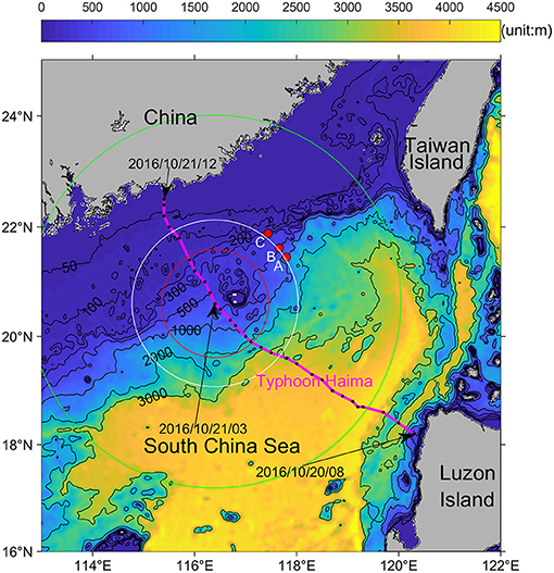
Figure 1. Map showing the bathymetry (color, unit: m) of the SCS and trajectory of Typhoon “Haima” (pink line). The pink color indicates that the intensity of this typhoon kept as Category One all the time in the SCS according to the Saffir-Simpson Hurricane Wind Scale. The three moorings (A, B, and C) are labeled with red dots. The black dots indicate the location of “Haima” every 1 h. Referring to the Beaufort wind scale, the red, white, and green circles represent the wind radii of Grade 12 (~100 km), Grade 10 (~160 km), and Grade 7 (~380 km), respectively, at 3:00 a.m. on October 21, 2016 when the typhoon center was closest to the mooring array.

TABLE 1

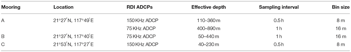
Table 1. Detailed information about the mooring ADCPs.

Typhoon Information

Typhoon “Haima” was generated in the Northwest Pacific at 8:00 a.m. on October 15, 2016. After entering the SCS at 10:00 a.m. on October 20, 2016, it moved northwestward at a speed of about ~27 km/h and kept its largest wind speed of ~42 m/s. When passing through the SCS, this typhoon maintained the level of Category One according to the Saffir–Simpson Hurricane Wind Scale (https://www.nhc.noaa.gov/aboutsshws.php). At around ~3:00 a.m. on October 21, the typhoon center was closest to the mooring array (~160 km; Figure 1). At that moment, the wind speed was about 35 m/s near the moorings A, B, and C. Additionally, the wind speed radii of Grade 12, Grade 10, and Grade 7 (referring to the Beaufort wind scale) were ~100, ~160, and ~380 km, respectively (Figure 1). After passing the mooring array, the typhoon landed at around 12:40 p.m. on October 21, 2016. All the information on Typhoon “Haima” is available on the China Meteorological Agency (http://typhoon.nmc.cn/web.html). The path of Typhoon “Haima” was almost parallel to the mooring array on the northeast side (Figure 1).

Reanalysis Currents Data

Three-dimensional currents data from the Copernicus Marine Environment Monitoring Service (CMEMS) were used to identify the BGF field. Their horizontal resolution was 1/12° × 1/12° (~8 km), with 50 vertical standard levels and a time interval of 1 day. This reanalysis product was based largely on the current real-time global forecasting CMEMS system. The model component was the Nucleus for European Modeling of the Ocean (NEMO) platform, which was driven at the surface by the European Center for Medium-Range Weather Forecasts (ECMWF) ERA-Interim reanalysis. The along-track altimeter data (sea level anomaly), satellite sea surface temperature, sea ice concentration, and in situ temperature, and salinity vertical profiles were jointly assimilated to the model by means of a reduced-order Kalman filter. The validity of these reanalysis current data can be identified by comparing with the ADCP data.

Bandpass Filtering

We first removed the anomalous values in raw current data and then, used the linear interpolation method to convert the data to the specified depth to obtain continuous currents at the same depth. In this study, we focused on the NIWs. A fourth-order Butterworth bandpass filter was applied to extract the near-inertial velocities. The cut-off frequency band is [0.85, 1.15]f₀, where f₀ is the local inertial frequency.

Computing Near-Inertial Kinetic Energy Density

The near-inertial kinetic energy density (NIKE) can be calculated as follows (Alford et al., 2012):

$\begin{array}{ll}\begin{array}{c}NIKE=\frac{1}{2}\rho \left(z\right)\left({u_f}^2+{v_f}^2\right)\end{array}& (1)\end{array}$

where ρ(z) is the seawater density that is calculated by 1/4° × 1/4° monthly mean climatological temperature and salinity data from the World Ocean Atlas 2018 (WOA18), and u_f and v_f are the near-inertial zonal and meridional velocities, respectively. The energy averaged over a wave period can better reflect the wave energy (Yang and Hou, 2014), so the sliding average of NIKE (hereafter, $\overline{NIKE}$) is carried out in the actual calculation.

Dynamic Modal Decomposition

In an ocean with a depth of H, the vertical structure of NIWs can be represented by the superposition of multiple discrete vertical modes (Alford and Zhao, 2007; Klymak et al., 2011; Ma et al., 2013; Shang et al., 2015) as follows:

$\begin{array}{ll}\begin{array}{c}u(z,t)={{\displaystyle \sum _{n=1}^{\infty }}{u}_n(z,t)}_{}\end{array}& (2)\end{array}$

$\begin{array}{ll}\begin{array}{c}{u}_n(z,t)={u_n(t)•\varnothing }_n(z)\end{array}& (3)\end{array}$

where u(z, t) is the velocity of NIWs (i.e., u_f or v_f), u_n(z, t) is the normal modal velocity, n is the number of modes, u_n(t) is the time coefficient that can be fitted by the least square method, and ∅_n(z) is the horizontal velocity structure. ∅_n(z) can be obtained by the following equation (Shang et al., 2015):

$\begin{array}{ll}\begin{array}{c}{\varnothing }_n(z)=\rho (z)C_n^2\frac{d{\eta }_n(z)}{dz}\end{array}& (4)\end{array}$

where C_n is the eigen speed of the nth baroclinic mode, and _ηn(z)is the vertical displacement. For low frequency internal waves (ω ≪ N, and N is buoyancy frequency), they are solutions to the following modal equations (Mackinnon and Gregg, 2003; Alford and Zhao, 2007; Alford, 2010, 2020):

$\begin{array}{ll}\begin{array}{c}\frac{{\partial }^2{\eta }_n(z)}{\partial z^2}+\frac{N^2(z)}{c_n^2}{\eta }_n(z)=0\end{array}& (5)\end{array}$

$\begin{array}{ll}\begin{array}{c}{N}^2(z)=-\frac{g}{{\rho }_0}•\frac{\partial \rho (z)}{\partial z}\end{array}& (6)\end{array}$

These are subject to the boundary conditions η(0) = η(−H) = 0. In these formulas, g is the acceleration due to gravity, and ρ₀ = 1,030 kg/m³ is a reference density. Over a flat bottom, the vertical structure of the waves only depends on the ocean stratification profile N²(z) (Alford and Zhao, 2007; Klymak et al., 2011; Ma et al., 2013; Shang et al., 2015). Due to the low vertical resolution of the thermohaline chains of moorings A, B, and C, the vertical distribution of the buoyancy frequency during observation cannot be calculated. The sensitivity calculations by Nash et al. (2005) and Alford and Zhao (2007) showed that the buoyancy frequency profiles calculated from observed data were very close to the climatological hydrographic profiles. Thus, N²(z) computed from the monthly climatological data from WOA18 was used to compute the modal function and the eigen speed of each mode. The velocity and displacement of each mode, u_n(z, t) and _{ηn(z, t)}, can be extracted from the observed velocity and displacement profiles by least-squares modal fitting (Alford, 2003; Nash et al., 2005; Alford and Zhao, 2007). The profiles of buoyancy frequency, vertical displacement, and horizontal velocity of moorings A, B, and C are shown in Supplementary Figure S1. There may be some problems in decomposing the flows into vertical modes over sloping topography, but examples of applying this method to the sloping topography were also common in previous work (e.g., Klymak et al., 2011; Ma et al., 2013; Shang et al., 2015). As the average slope of our observed sea area is only about 3°, assuming a flat bottom is fairly reasonable.

Results

Characteristics of Observed NIWs

Before Typhoon “Haima” passed through the mooring array, from October 15 to 20, the near-inertial velocities were small (<5 cm/s; Figure 2). After Typhoon “Haima” passed over the mooring array (on October 24), the near-inertial velocities were significantly enlarged at all moorings, with the maximum velocity being more than 50 cm/s (Figure 2). At moorings A and B, strong NIWs successively appeared twice following Typhoon “Haima” (Figures 2A–D, 3A,B). The first event persisted until November 1. Hereafter, this period (from October 24 to November 1) is referred to as Stage-1. The second event started on November 3 and persisted until November 17. Hereafter, the latter period (from November 3 to November 17) is referred to as Stage-2. The enhanced NIWs were not observed at mooring C at Stage-2 (Figures 2E,F, 3C).

FIGURE 2

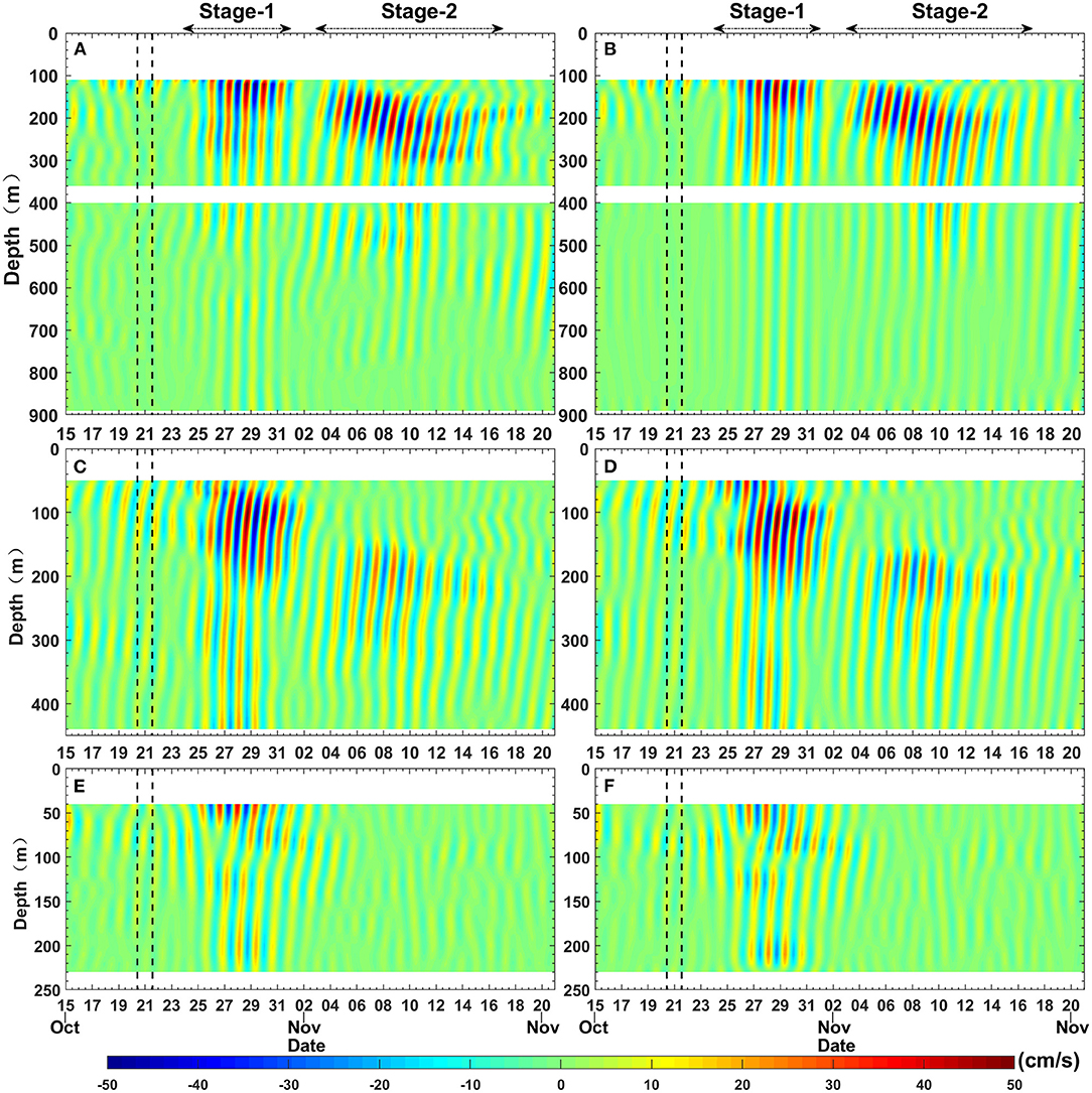
Figure 2. (Left) The time-depth graph of the band-pass ([0.85, 1.15] f₀) filtered near-inertial (meridional) velocities (unit: centimeter/second) from October 15 to November 20, 2016 at mooring A (A), mooring B (C), and mooring C (E). (Right) The sum of the first eight modes computed from the dynamic modal decomposition of the filtered near-inertial (meridional) velocities at mooring A (B), mooring B (D), and mooring C (F). The black dotted lines show the passage period of Typhoon “Haima”.

FIGURE 3

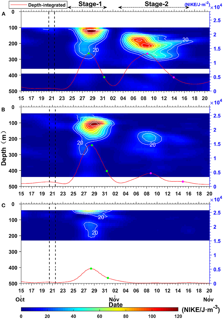
Figure 3. The time-depth graphs of moving-average near-inertial kinetic energy density ($\overline{NIKE}$) (unit: J/m³) at mooring A (A), mooring B (B), and mooring C (C). The red curves show the time evolution of the depth-integrated ($\overline{NIKE}$) (unit: J/m²) of the observation depth. The green and pink solid dots on each curve are the time interval which is used to compute the energy decays of NIWs (i.e., e-folding time scales). The black dotted lines show the passage period of Typhoon “Haima”. Contours start at 20 J/m³ and are displayed at an interval of 10 J/m³.

At Stage-1, strong NIWs showed a typical upward phase propagation and a downward energy propagation at all three moorings (Figure 2). On the continental slope (mooring A), strong NIWs appeared in the upper 200 m, below which the near-inertial energy fast decreased (Figure 3A). Compared with mooring A, NIWs on the shelf break (mooring B) showed comparable velocity amplitudes at the same depths, indicating similar responses to the typhoon at these two moorings. Near the continental shelf (mooring C), the NIWs were weaker than those on the continental slope and the shelf break. In the initial stage (October 26–29), an opposite phase (quasi-mode-1 structure) between the upper and lower layers can be observed at mooring C, which is a common near-inertial feature of ocean response to wind on a shallow sea (Sun Z. et al., 2011; Chen et al., 2015). After October 29, downward-traveling near-inertial signals can be clearly identified (Figure 2E). At Stage-2, the NIWs were weaker than those observed at Stage-1, especially at mooring B. In this period, the strong NIWs at both moorings appeared at deeper depths (140–360 m; Figures 2A–D, 3A,B), with the maximum energy occurring near 200 m.

Before Typhoon “Haima,” near-inertial velocity shears ($S=\sqrt{|\frac{\partial u}{\partial z}{|}^2+|\frac{\partial v}{\partial z}{|}^2}$) were identifiable, especially at mooring C (Figure 4C). The enhanced wind field before “Haima” arrived at the mooring array may have induced NIWs at the moorings. However, the shear can be elevated by more than four times 2–3 days after “Haima” traveled over the continental slope (Figure 4). Large near-inertial shears were also observed at Stage-2 at mooring A (Figure 4A). Below 150 m, the near-inertial velocity shears in this period were much larger than those observed at Stage-1, although the near-inertial velocity magnitude at Stage-2 was comparable to that at Stage-1. This suggested that the NIWs had smaller vertical scales at Stage-2 than at Stage-1. Additionally, the near-inertial velocities at mooring B were much smaller at Stage-2 than at Stage-1 in the subsurface layer, but the shears were larger at Stage-2. These near-inertial velocity shears were eventually able to extract and dissipate the energy of waves (Xie et al., 2009; Fer, 2014; Zhang et al., 2014), enabling the production of turbulence and associated deep small-scale vertical mixing (Kunze, 1985; Fer, 2014).

FIGURE 4

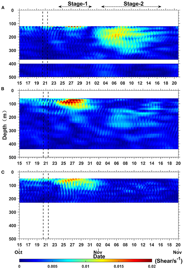
Figure 4. Time-depth graphs of near-inertial velocity shear at mooring A (A), mooring B (B), and mooring C (C). The black dotted lines show the passage period of Typhoon “Haima”.

The time evolution of the depth-integrated $\overline{NIKE}$ showed that the calculated e-folding time scales of moorings A, B, and C at Stage-1 were 2.3, 2.2, and 2.4 times those of the local inertial period—namely, 2.3/f ₀ (74 h), 2.2/f ₀ (69 h), and 2.4/f ₀ (77.5 h), respectively. Such small e-folding time scales indicate that $\overline{NIKE}$ was attenuated at a fast rate. One should note that the e-folding time scale does not mean the rate of local dissipation, but rather how fast the total near inertial-energy reduced in the observed time series. It contains both the portion of energy that propagated away from the mooring and the portion of local dissipation that occurred due to turbulent mixing and other interaction. Therefore, the advection of the wave packet away from the mooring array could also account for the observed small e-folding time scales. At Stage-2, the $\overline{NIKE}$ at mooring B was nearly half the $\overline{NIKE}$ at mooring A. At mooring A, the $\overline{NIKE}$ at Stage-2 was comparable with that at Stage-1, while the $\overline{NIKE}$ at mooring B at Stage-2 was much weaker than that at Stage-1 (<1/3). The e-folding time scales of $\overline{NIKE}$ at moorings A and B were 3.8/f ₀ (125 h) and 4.5/f ₀ (148 h) at Stage-2, respectively, suggesting that $\overline{NIKE}$ decays more slowly at Stage-2 than at Stage-1.

Dynamic Modal Analysis

In the above section, the observations showed that the vertical scales of NIWs at both A and B were smaller at Stage-2 than at Stage-1, suggesting the dominance of higher vertical modes at Stage-2. To quantify the modal contents, we performed dynamic modal decomposition. The sum of the first eight modes could well reproduce the near-inertial velocity patterns at both Stage-1 and Stage-2 (Figure 2). The contributions of these eight modes to the total near inertial velocity are shown in Figure 5.

FIGURE 5

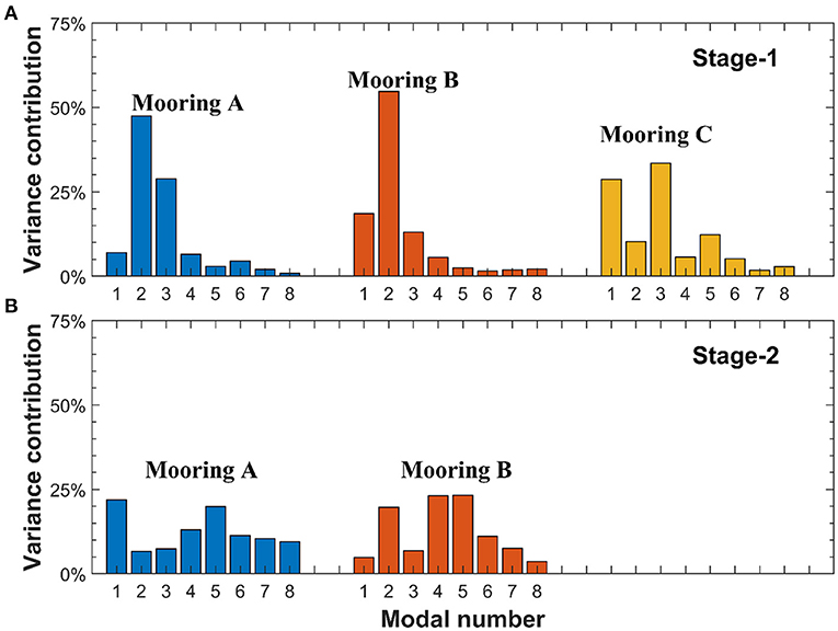
Figure 5. The percentages of the first eight modes at three moorings at Stage-1 (A) and Stage-2 (B).

The modal contents at Stage-1 and Stage-2 were different. At Stage-1, the NIWs were dominated by the first three modes, which can explain ~83, ~87, and ~75% of the total velocity variance at moorings A, B, and C, respectively. However, the maximum mode was different on the continental shelf and slope. Mode-2 on the continental slope and the shelf break (A and B) had the largest energy, while mode-1 and mode-3 had comparable energies at mooring C near the continental shelf and contributed ~65% of the total variance. At Stage-2, the sum of the contribution of the first three modes decreased significantly and the importance of the higher modes began to work. Compared to Stage-1 (<17% for the sum of 4–8 modes), higher modes (n > 3) became dominant and explained ~64% and ~69% of the total energy at A and B, respectively, as shown in the near-inertial shear field. The low-mode NIWs (modes 1–3) can quickly propagate thousands of kilometers away (preferentially equatorward), while the NIWs of higher modes remain to eventually dissipate since they are more likely to break during the propagation (Alford and Zhao, 2007; Alford, 2020). Therefore, the NIWs of higher modes at Stage-2 could be advected from nearby lower latitudes by the BGF. We will further explore this issue in the discussion section.

Frequency Estimation of NIWs

In addition to the different modal contents, the frequencies of the NIWs at Stage-1 and Stage-2 were also different. To calculate the frequencies of NIWs, the band-pass-filtered near-inertial velocity was fitted into the following equation:

$\begin{array}{ll}\begin{array}{c}u(z,t)=v_0+a\; •\; sin\left(2\pi f_{i}t+\theta \right)+E(t)\end{array}& (7)\end{array}$

where f_i is the test frequency; v₀, a, and θ are the fitting parameters; and E(t) is the residual error (Rossby and Sanford, 1976; Shay and Elsberry, 1987; Jaimes and Shay, 2010; Sun Z. et al., 2011; Pallàs-Sanz et al., 2015). A common combined measure of the quality of fitting for near-inertial velocity is (Jaimes and Shay, 2010; Pallàs-Sanz et al., 2015):

$\begin{array}{ll}\begin{array}{c}R=\sqrt{\frac{r_u^2+r_v^2}{2}}\end{array}& (8)\end{array}$

where r_u and r_v are the correlation coefficients between the observed and modeled components of the velocity, respectively. This study results show that R is mostly >0.9 (see Supplementary Figure S2), which indicates that the fitting results are reliable.

The near-inertial frequencies at different depths are shown in Figure 6 and the depth-mean near-inertial frequencies of the corresponding depth range are shown in Table 2. The results showed that the near-inertial frequency was much lower at Stage-2 than at Stage-1 in both zonal and meridional velocities (Figure 6). At Stage-1, the frequencies of the NIWs at all moorings were blue-shifted with respect to the local inertial frequencies. Such a frequency shift of NIWs can commonly be observed during tropical cyclones. Furthermore, three moorings presented a similar variance with depth. However, the “blue-shift” value at each mooring was different. The magnitudes of the “blue-shift” at moorings A and B were relatively large, and the frequencies of the observed NIWs at these two moorings were ~1.05 f , while the frequency was ~1.03 f at mooring C (Table 2). On the contrary, the frequencies of NIWs at both moorings A and B were red-shifted to ~0.98 f at Stage-2. As the depth increased, the red-shift was reduced (Figures 6D,E).

FIGURE 6

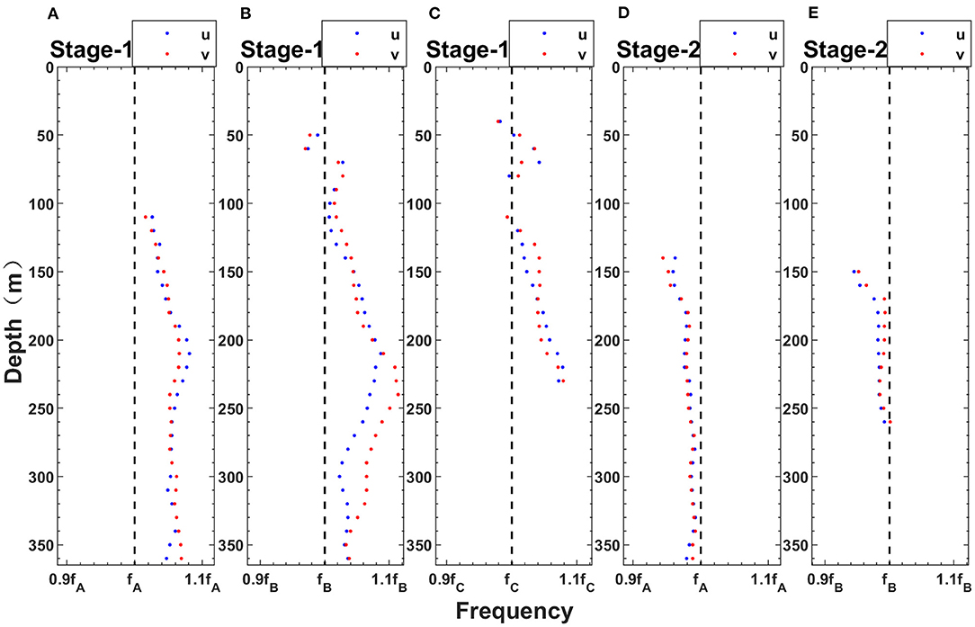
Figure 6. Ratio of the frequency of observed NIWs and the local inertial frequency versus depth at Stage-1 (A–C) and Stage-2 (D, E) at mooring A (A, D), mooring B (B, E), and mooring C (C). Note that the results at depths with very small ($\overline{NIKE}$) (<15 J/m³) are removed. The blue dots and red dots represent the frequencies of the zonal and meridional velocities of NIWs, respectively. The black dashed line represents the local inertial frequency at each mooring.

TABLE 2

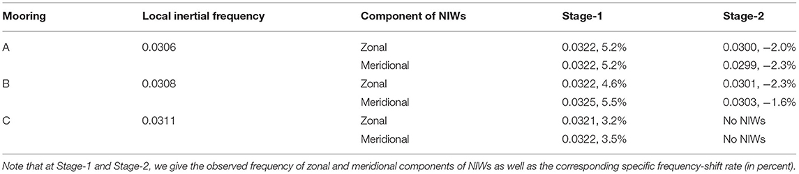
Table 2. Detailed information about the frequency (unit: cph).

Discussion

The blue-shift feature of NIWs is common in the ocean and can be predicted by the linear internal wave dynamics (Fu, 1980). Although the red-shifted NIWs are also often observed, their occurrence following tropical cyclones is rare. A common explanation for red-shifted NIWs is the effect of the mean flow including background vorticity (Kunze, 1985; Sun Z. et al., 2011; Chen et al., 2015) and Doppler shift (Pallàs-Sanz et al., 2015; Sun et al., 2015; Jeon et al., 2019). The theories and observations have shown that the background vorticity ζ could shift the lower bound of the internal wave band from f₀ to an effective Coriolis frequency f_eff (Kunze, 1985; Sun et al., 2015; Xie et al., 2015; Alford et al., 2016). In the stratified flows with the absence of vertical shear, the actual observed frequency ω satisfies the following equations (Claret and Viúdez, 2010; Pallàs-Sanz et al., 2015):

$\begin{array}{ll}\begin{array}{c}\omega =\sqrt{N^2\frac{k^2+l^2}{k^2+l^2+m^2}+{f_{eff}}^2\frac{m^2}{k^2+l^2+m^2}}+\text{K}•\overline{\text{V}}\end{array}& (9)\end{array}$

$\begin{array}{ll}\begin{array}{c}{f}_{eff}\approx f_0+\frac{\zeta }{2}\end{array}& (10)\end{array}$

$\begin{array}{ll}\begin{array}{c}\zeta =\frac{\partial \overline{v}}{\partial x}-\frac{\partial \overline{u}}{\partial y}\end{array}& (11)\end{array}$

where K = (k, l, m) is the wave number vector and $\overline{\text{V}}=(\overline{u}, v, \overline{w})$ is the mean BGF. When ζ is negative, sub-inertial NIWs may be trapped (Kawaguchi et al., 2020). In order to confirm the potential influence of background vorticity, we used the reanalysis currents data from the CMEMS to calculate the background vorticity. The validity of these reanalysis current data can be identified by comparing them with ADCP data (e.g., Figure 9).

Since large NIWs were observed above 360 m at both Stage-1 and Stage-2, reanalysis current data in this depth range were used to calculate the relative vorticity (Figure 7). We adopted the average vorticity of the 1° × 1° region (moorings A, B, and C were in the same 1° × 1° region) to represent the background vorticity of the moorings. Before and during the typhoon passage, the vorticity was positive but became negative during strong near-inertial events. The time-mean ζ/2 was approximately −7.04 × 10⁻⁴ cph at Stage-1, while it was −6.32 × 10⁻⁴ cph at Stage-2. That is, f_eff was ~0.98 f at moorings A and B, and it was close to the frequency of the NIWs observed at Stage-2. Therefore, it was possible that the sub-inertial waves observed at Stage-2 were due to the effects of the negative background vorticity. However, we should assume that these waves were generated during the typhoon passage and at that time, the relative vorticity was positive; thus, the NIWs should be super-inertial, meaning that the sub-inertial waves could not be locally generated. Instead, they may have resulted from lower latitudes where they were generated with respect to the local inertial frequency of the generated location and propagated poleward to the moorings. As a result, the frequencies of these waves became sub-inertial due to the β-effect (the intrinsic frequency ω of waves does not change, but f increases with latitude, thus gradually ω < f).

FIGURE 7

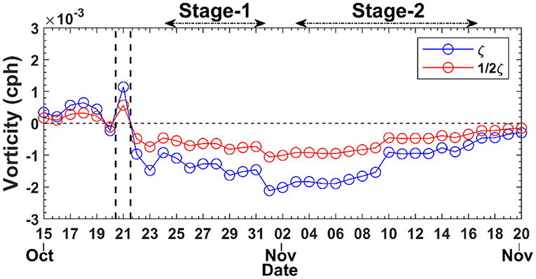
Figure 7. The temporal evolution of background vorticity at three moorings before and after the passage of Typhoon “Haima.” The vertical black dotted lines show the passage period of Typhoon “Haima.” We adopt the average vorticity of the 1° × 1° region (moorings A, B, and C were located in the same 1° × 1° region) to represent the background vorticity of moorings.

In the absence of poleward BGF, NIWs could not propagate from the generated location to our moorings whose latitudes were higher than their critical latitudes. However, the observed poleward BGF allowed the possibility of the poleward propagation of these NIWs to the moorings. The previous studies have also revealed that the waves can propagate poleward beyond their critical latitude under the effect of the mean flow (Zhai et al., 2005; Gerkema et al., 2013; Xie et al., 2015). Therefore, the poleward propagation of NIWs may be associated with the poleward BGF caused by typhoons (Figures 8, 9). In Equation (9), the second term $\text{K}•\overline{\text{V}}$ can also account for the “red-shift” frequencies of NIWs if the mean flow is poleward (Gerkema et al., 2013; Xie et al., 2015). However, the time–depth map of the low-pass-filtered meridional velocity at A and B showed that the mean flows at Stage-2 were not always poleward (Figures 8A,B). In contrast, the strong poleward BGFs caused by “Haima” were observed at Stage-1 (Figures 8, 9). Furthermore, the reanalysis current data showed that the BGF in a large area to the south of moorings A and B was almost poleward following “Haima” (October 27–November 8; Figure 9). Therefore, these poleward BGF may accelerate the propagation of “Haima” -induced poleward traveling NIWs and reverse the equatorward propagation component (Zhai et al., 2005; Xie et al., 2015). Xie et al. (2015) have suggested that the high-mode waves may be more easily advected by BGF because of their relatively small propagation speed. Under the effect of a meridional BGF, the meridional group velocity of NIWs (Xie et al., 2015) is

$\begin{array}{ll}\begin{array}{c}{C}_{gy}=\overline{v}+\frac{C_n^{2}l}{(\omega -l\overline{v})}\end{array}& (12)\end{array}$

FIGURE 8

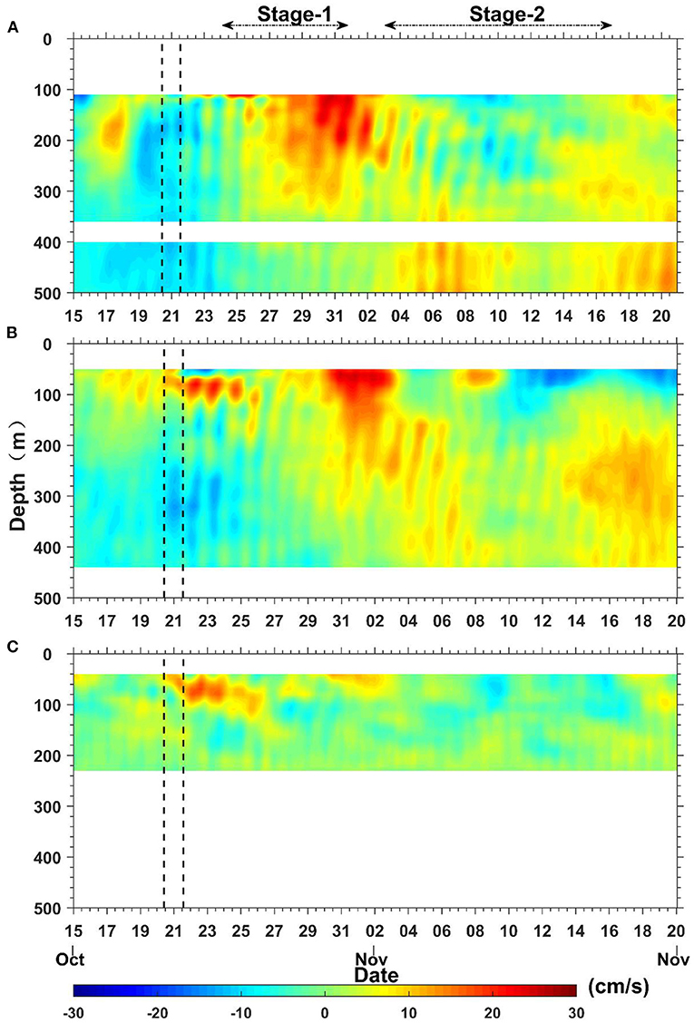
Figure 8. The time-depth graph of low-pass filtered (96 h) meridional velocities (unit: cm/s) obtained at mooring A (A), mooring B (B), and mooring C (C) from October 15 to November 20, 2016. The black dotted lines show the passage period of Typhoon “Haima”.

FIGURE 9

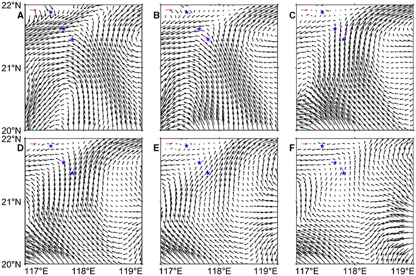
Figure 9. Map of the mean BGF (unit: cm/s) of 100–360 m depth on (A) October 23, (B) October 27, (C) October 31, (D) November 4, (E) November 8, and (F) November 12. The blue stars indicate the mooring locations as Figure 1 shows. The red arrow at the top left corner of each panel indicates the velocity due east at 10 cm/s. The pink arrows indicate the mean observed velocity between 100 and 360 m depth at moorings.

To confirm whether high-mode NIWs can be transported poleward by the BGF, we computed Equation (12) based on the mooring and reanalysis data. The results showed that the low-mode (modes 1–3) NIWs have a relatively large baroclinic dispersion term [the second term on the right side of Equation (12)]; therefore, they can overcome advection (Figure 10) and freely propagate (preferentially equatorward). They can even propagate quickly thousands of kilometers away (Alford and Zhao, 2007; Alford, 2020). However, as the vertical wavenumber increases, the mean flow velocity exceeds the baroclinic dispersion speed when n > 3 (Figure 10). Therefore, the high-mode NIWs can be carried away by the poleward BGF to other regions with different latitudes. This explains why high-mode NIWs were dominant at Stage-2.

FIGURE 10

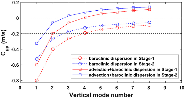
Figure 10. Horizontal group velocity as a function of vertical mode number computed from Equation (12) (line with squares) and the baroclinic dispersion term in Equation (12) (line with circles). Red color and blue color represent Stage-1 and Stage-2, respectively.

The previous studies have suggested that the low-mode NIWs (modes 1–3) can quickly propagate thousands of kilometers away (preferentially equatorward) while the high mode NIWs remain to eventually dissipate since they are more likely to break during the propagation (Alford and Zhao, 2007; Alford, 2020). The high mode NIWs are easily dissipated, but it does not mean that they must completely vanish within a short distance from the generation site. They can still travel a certain distance (tens to hundreds of kilometers), especially under the effects of the favorable BGF. But they cannot travel very far since they will dissipate very quickly because of their potential shear instability in the presence of high velocity shears (Figure 4). As shown in Figure 3, when near-inertial waves observed at Stage-2 traveled poleward to mooring A, they still had large kinetic energy. However, when they arrived at mooring B, their energy became much smaller. Note that the distance between A and B is only ~20 km (Figure 1), suggesting significant energy dissipation during their poleward propagation with a short distance. The NIWs were not observed at mooring C at Stage-2 (Figures 2E,F, 3C) because they likely dissipated completely before they propagated poleward to mooring C.

Conclusions

Based on the observations of three moorings in the northern SCS, this article analyzes the responses of the upper ocean at the continental slope, shelf break, and continental shelf to Typhoon “Haima” and the poleward propagation of typhoon-induced NIWs.

Moorings with different locations responded differently to the typhoon, with stronger NIWs on the continental slope to the shelf break and relatively weak NIWs near the shallow continental shelf. The frequencies of the NIWs at all these three moorings at Stage-1 were super-inertial, and the level of “blue-shift” of NIWs at moorings A and B at Stage-1 could be more than 5%, while it was only ~3.5% at mooring C. Moreover, the NIWs at all these three moorings at Stage-1 were mainly dominated by the first three baroclinic modes, and the energy of these low modes can quickly spread away under the influence of the baroclinic dispersion term and the BGF.

After the NIWs observed at Stage-1 had decayed completely due to their propagation away and local dissipation, strong NIWs were again observed at moorings A and B at Stage-2. The analysis of the mean BGF reveals that these NIWs were excited at lower latitudes, and then, reached moorings A and B by the advection of the BGF. Therefore, frequencies at Stage-2 presented a “red-shift” effect relative to the local inertial frequencies. However, no NIWs were observed at mooring C at Stage-2, as mooring C was located further north near the continental shelf and there was no persistent poleward BGF there. Therefore, NIWs could not arrive at mooring C since they had dissipated completely during the poleward propagation to mooring C. Additionally, a theoretical analysis shows that low-mode (n ≤ 3) NIWs can overcome the effect of advection and freely propagate, while the higher-mode (n > 3) NIWs are more easily carried away by BGF to other regions. Therefore, NIWs at Stage-2 have a large contribution of higher modes. During poleward propagation, the red-shifted NIWs propagated downward and dissipated energy because of their potential shear instability in the presence of high velocity shears. Therefore, the NIWs at Stage-2 appeared to be deeper, and the observed $\overline{NIKE}$ was larger at mooring A than that at mooring B.

These findings emphasize the fact that the BGF plays a significant role in the redistribution of energy in the upper ocean imported from tropical cyclones, as the BGF can enable NIWs to propagate poleward and reach areas with higher latitudes than the critical latitude. The previous observational and modeling studies have suggested that the typhoon-induced NIWs may be a common phenomenon that occurs frequently in the ocean. Given the fact that the typhoon-induced NIW energy may be redistributed to non-source region to drive turbulent mixing there, one should not ignore the impact of BGF on the NIW energy redistribution when considering the energy budget in climate and Earth system models.

Data Availability Statement

Mooring data sufficient to regenerate the figures, tables, and other results in this paper are stored on computers of Xiamen University, and can be freely available at https://dspace.xmu.edu.cn/handle/2288/174152. All the information of Typhoon “Haima” used in this paper is available on the China Meteorological Agency (http://typhoon.nmc.cn/web.html). Temperature and salinity data from the World Ocean Atlas 2018 (WOA18) can be downloaded from https://www.nodc.noaa.gov/OC5/woa18/. And the reanalysis current data can be accessed through Copernicus Marine Service (https://resources.marine.copernicus.eu/?option=com_csw&view=details&product_id=GLOBAL_REANALYSIS_PHY_001_030).

Author Contributions

JH and ZS designed the experiment and secured funding. ZS conducted the fieldwork. RH processed the data and performed analyses with guidance from XX, JH, and ZS. RH wrote the manuscript, with significant input from XX and JH. All the authors contributed to the article and approved the submitted version.

Funding

This study was jointly supported by the National Natural Science Foundation of China (91958203 and 41776027). XX was also supported by the Scientific Research Fund of the Second Institute of Oceanography, the MNR (HYGG2003), the Natural Science Foundation of Zhejiang (LR20D060001), the NSFC (41876016), and the MEL Visiting Fellowship (MELRS1913). RH was supported by The PhD Fellowship of the State Key Laboratory of Marine Environmental Science at Xiamen University.

Conflict of Interest

The authors declare that the research was conducted in the absence of any commercial or financial relationships that could be construed as a potential conflict of interest.

Publisher's Note

All claims expressed in this article are solely those of the authors and do not necessarily represent those of their affiliated organizations, or those of the publisher, the editors and the reviewers. Any product that may be evaluated in this article, or claim that may be made by its manufacturer, is not guaranteed or endorsed by the publisher.

Acknowledgments

We acknowledge all the principal investigators and technicians, as well as the captain and crew of R/V Yanping 2, for deploying and recovering the in-situ moorings, without whose talent and hard work, the observation would not be possible. We also thank the valuable comments and the nice suggestions from Gilles Reverdin, Ilker Fer, and other reviewers that help improve the article.

Supplementary Material

The Supplementary Material for this article can be found online at: https://www.frontiersin.org/articles/10.3389/fmars.2021.713991/full#supplementary-material

References

Alford, M. H. (2001). Internal swell generation: the spatial distribution of energy flux from the wind to mixed layer near-inertial motions. J. Phys. Oceanogr. 231, 2359–2368. doi: 10.1175/1520-0485(2001)031<2359:ISGTSD>2.0.CO

CrossRef Full Text | Google Scholar

Alford, M. H. (2003). Redistribution of energy available for ocean mixing by long-range propagation of internal waves. Nature 423, 159–162. doi: 10.1038/nature01628

PubMed Abstract | CrossRef Full Text | Google Scholar

Alford, M. H. (2010). Sustained, full-water-column observations of internal waves and mixing near Mendocino Escarpment. J. Phys. Oceanogr. 40, 2643–2660. doi: 10.1175/2010JPO4502.1

CrossRef Full Text | Google Scholar

Alford, M. H. (2020). Global calculations of local and remote near-inertial-wave dissipation. J. Phys. Oceanogr. 50, 3157–3164. doi: 10.1175/JPO-D-20-0106.1

CrossRef Full Text | Google Scholar

Alford, M. H., Cronin, M. F., and Klymak, J. M. (2012). Annual cycle and depth penetration of wind-generated near-inertial internal waves at ocean station Papa in the northeast pacific. J. Phys. Oceanogr. 42, 889–909. doi: 10.1175/JPO-D-11-092.1

CrossRef Full Text | Google Scholar

Alford, M. H., and Gregg, M. C. (2001). Near-inertial mixing: modulation of shear, strain and microstructure at low latitude. J. Geophys. Res. Oceans 106, 16947–16968. doi: 10.1029/2000JC000370

CrossRef Full Text | Google Scholar

Alford, M. H., Mackinnon, J. A., Simmons, H. L., and Nash, J. D. (2016). Near-inertial internal gravity waves in the ocean. Annu. Rev. Marine Sci. 8, 95–123. doi: 10.1146/annurev-marine-010814-015746

PubMed Abstract | CrossRef Full Text | Google Scholar

Alford, M. H., Shcherbina, Y. A., and Gregg, C. M. (2013). Observations of near-inertial internal gravity waves radiating from a frontal jet. J. Phys. Oceanogr. 43, 1225–1239. doi: 10.1175/JPO-D-12-0146.1

CrossRef Full Text | Google Scholar

Alford, M. H., and Zhao, Z. (2007). Global patterns of low-mode internal-wave propagation. Part I: energy and energy flux. J. Phys. Oceanogr. 37, 1829–1848. doi: 10.1175/JPO3085.1

CrossRef Full Text | Google Scholar

Boyer, A. L., Alford, M. H., Pinkel, R., Hennon, T. D., Yang, Y. J., Ko, D., and Nash, J. D. (2020). Frequency shift of near-inertial waves in the South China Sea. J. Phys. Oceanogr. 50, 1121–1135. doi: 10.1175/JPO-D-19-0103.1

CrossRef Full Text | Google Scholar

Cao, A., Guo, Z., Song, J., Lv, X., He, H., and Fan, W. (2018). Near-inertial waves and their underlying mechanisms based on the South China Sea internal wave experiment (2010–2011). J. Geophys. Res. Oceans 123, 5026–5040. doi: 10.1029/2018JC013753

CrossRef Full Text | Google Scholar

Chen, G., Xue, H., Wang, D., and Xie, Q. (2013). Observed near-inertial kinetic energy in the northwestern South China Sea. J. Geophys. Res. Oceans 118, 4965–4977. doi: 10.1002/jgrc.20371

CrossRef Full Text | Google Scholar

Chen, K. (2007). Typhoon induced inertial motion in the South China Sea (dissertation). National Taiwan University, Taipei, Taiwan. p. 98.

Chen, S., Hu, J., and Polton, J. A. (2015). Features of near-inertial motions observed on the northern South China Sea shelf during the passage of two typhoons. Acta Oceanol. Sin. 34, 38–43. doi: 10.1007/s13131-015-0594-y

CrossRef Full Text | Google Scholar

Claret, M., and Viúdez, Á. (2010). Vertical velocity in the interaction between inertia-gravity waves and sub-mesoscale baroclinic vortical structures. J. Geophys. Res. Oceans 115:C12060. doi: 10.1029/2009JC005921

CrossRef Full Text | Google Scholar

D'Asaro, E. A. (1985). The energy flux from the wind to near-inertial motions in the surface mixed layer. J. Phys. Oceanogr. 15, 1043–1059. doi: 10.1175/1520-0485(1985)015<1043:TEFFTW>2.0.CO

CrossRef Full Text | Google Scholar

Fer, I. (2014). Near-inertial mixing in the central Arctic Ocean. J. Phys. Oceanogr. 44, 2031–2049. doi: 10.1175/JPO-D-13-0133.1

CrossRef Full Text | Google Scholar

Fer, I., Bosse, A., Ferron, B., and Bouruet-Aubertot, P. (2018). The dissipation of kinetic energy in the Lofoten Basin Eddy. J. Phys. Oceanogr. 48, 1299–1316. doi: 10.1175/JPO-D-17-0244.1

CrossRef Full Text | Google Scholar

Fu, L. L. (1980). Observations and models of inertial waves in the deep ocean. Rev. Geophys. 19, 141–170. doi: 10.1029/RG019i001p00141

CrossRef Full Text | Google Scholar

Garrett, C. (2003). Oceanography: mixing with latitude. Nature 422, 477–478. doi: 10.1038/422477a

PubMed Abstract | CrossRef Full Text | Google Scholar

Gerkema, T., Maas, L. R. M., and Haren, H. V. (2013). A note on the role of mean flows in Doppler-shifted frequencies. J. Phys. Oceanogr. 43, 432–441. doi: 10.1175/JPO-D-12-090.1

CrossRef Full Text | Google Scholar

Gill, A. E. (1982). Atmosphere–Ocean Dynamics. New York, NY: Academic Press. p. 662.

Guan, S., Zhao, W., Huthnance, J., Tian, J., and Wang, J. (2014). Observed upper ocean response to typhoon Megi (2010) in the Northern South China Sea. J. Geophys. Res. Oceans 119, 3134–3157. doi: 10.1002/2013JC009661

CrossRef Full Text | Google Scholar

Jaimes, B., and Shay, L. K. (2010). Near-inertial wave wake of Hurricanes Katrina and Rita over mesoscale oceanic eddies. J. Phys. Oceanogr. 40, 1320–1337. doi: 10.1175/2010JPO4309.1

CrossRef Full Text | Google Scholar

Jeon, C., Park, J., Nakamura, H., Nishina, A., Zhu, X. H., Kim, D. G., et al. (2019). Poleward-propagating near-inertial waves enabled by the western boundary current. Sci. Rep. 9, 1977–2010. doi: 10.1038/s41598-019-46364-9

PubMed Abstract | CrossRef Full Text | Google Scholar

Kawaguchi, Y., Wagawa, T., and Igeta, Y. (2020). Near-inertial internal waves and multiple-inertial oscillations trapped by negative vorticity anomaly in the central Sea of Japan. Progress Oceanogr. 181:102240. doi: 10.1016/j.pocean.2019.102240

CrossRef Full Text | Google Scholar

Klymak, J. M., Alford, M. H., Pinkel, R., Lien, R., Yang, Y. J., and Tang, T. (2011). The breaking and scattering of the internal tide on a continental slope. J. Phys. Oceanogr. 41, 926–945. doi: 10.1175/2010JPO4500.1

CrossRef Full Text | Google Scholar

Kunze, E. (1985). Near-inertial wave propagation in geostrophic shear. J. Phys. Oceanogr. 15, 544–565. doi: 10.1175/1520-0485(1985)015<0544:NIWPIG>2.0.CO

CrossRef Full Text | Google Scholar

Ma, B., Lien, R., and Dong, S. (2013). The variability of internal tides in the Northern South China Sea. J. Oceanogr. 69, 619–630. doi: 10.1007/s10872-013-0198-0

CrossRef Full Text | Google Scholar

Mackinnon, J. A., and Gregg, M. C. (2003). Shear and baroclinic energy flux on the summer new England shelf. J. Phys. Oceanogr. 33, 1462–1475. doi: 10.1175/1520-0485(2003)033<1462:SABEFO>2.0.CO

CrossRef Full Text | Google Scholar

Maeda, A., Uejima, K., Yamashiro, T., Sakurai, M., Ichikawa, H., Chaen, M., et al. (1996). Near inertial motion excited by wind change in a margin of the Typhoon 9019. J. Oceanogr. 52, 375–388. doi: 10.1007/BF02235931

CrossRef Full Text | Google Scholar

Nash, J. D., Alford, M. H., and Kunze, E. (2005). Estimating internal-wave energy fluxes in the ocean. J. Atm. Oceanic Technol. 22, 1551–1570. doi: 10.1175/JTECH1784.1

CrossRef Full Text | Google Scholar

Oey, L. Y., Inoue, M., Lai, R., Lin, X. H., Welsh, S. E., and Rouse, L. J. (2008). Stalling of near-inertial waves in a cyclone. Geophys. Res. Lett. 35, 150–152. doi: 10.1029/2008GL034273

CrossRef Full Text | Google Scholar

Pallàs-Sanz, E., Candela, J., Sheinbaum, J., Ochoa, J., and Jouanno, J. (2015). Trapping of the near-inertial wave wakes of two consecutive hurricanes in the loop current. J. Geophys. Res. Oceans 121, 7431–7454. doi: 10.1002/2015JC011592

CrossRef Full Text | Google Scholar

Price, J. F., Sanford, T. B., and Forristall, G. Z. (1994). Forced stage response to a moving hurricane. J. Phys. Oceanogr. 24, 233–260. doi: 10.1175/1520-0485(1994)024<0233:FSRTAM>2.0.CO

CrossRef Full Text | Google Scholar

Rossby, H. T., and Sanford, T. B. (1976). A study of velocity profiles through the main thermocline. J. Phys. Oceanogr. 6, 766–774. doi: 10.1175/1520-0485(1976)006<0766:ASOVPT>2.0.CO

CrossRef Full Text | Google Scholar

Rubino, A., Dotsenko, S., and Brandt, P. (2010). Near-inertial oscillations of geophysical surface frontal currents. J. Phys. Oceanogr. 33, 1990–1999. doi: 10.1175/1520-0485(2003)033<1990:NOOGSF>2.0.CO

CrossRef Full Text | Google Scholar

Shang, X., Liu, Q., Xie, X., Chen, G., and Chen, R. (2015). Characteristics and seasonal variability of internal tides in the southern South China Sea. Deep Sea Res. Part I 98, 43–52. doi: 10.1016/j.dsr.2014.12.005

CrossRef Full Text | Google Scholar

Shay, L. K., and Elsberry, R. L. (1987). Near-inertial ocean current response to Hurricane Frederic. J. Phys. Oceanogr. 17, 1249–1269. doi: 10.1175/1520-0485(1987)017<1249:NIOCRT>2.0.CO

CrossRef Full Text | Google Scholar

Sun, L., Zheng, Q., Tang, T. Y., Chuang, W. S., Li, L., Hu, J., et al. (2012). Upper ocean near-inertial response to 1998 Typhoon “faith” in the South China Sea. Acta Oceanol. Sin. 31, 25–32. doi: 10.1007/s13131-012-0189-9

CrossRef Full Text | Google Scholar

Sun, Z., Hu, J., Zheng, Q., and Gan, J. (2015). Comparison of typhoon-induced near-inertial oscillations in shear flow in the northern South China Sea. Acta Oceanol. Sin. 34, 38–45. doi: 10.1007/s13131-015-0746-0

CrossRef Full Text | Google Scholar

Sun, Z., Hu, J., Zheng, Q., and Li, C. (2011). Strong near-inertial oscillations in geostrophic shear in the northern South China Sea. J. Oceanogr. 67, 377–384. doi: 10.1007/s10872-011-0038-z

CrossRef Full Text | Google Scholar

Xie, X., Liu, Q., Shang, X., Chen, G., and Wang, D. (2015). Poleward propagation of parametric subharmonic instability-induced inertial waves. J. Geophys. Res. Oceans 121, 1881–1895. doi: 10.1002/2015JC011194

CrossRef Full Text | Google Scholar

Xie, X., Shang, X., Chen, G., and Sun, L. (2009). Variations of diurnal and inertial spectral peaks near the bi-diurnal critical latitude. Geophys. Res. Lett. 36, 349–363. doi: 10.1029/2008GL036383

CrossRef Full Text | Google Scholar

Xu, J., Huang, Y., Chen, Z., Liu, J., and Ning, D. (2019). Horizontal variations of typhoon-forced near-inertial oscillations in the South China Sea simulated by a numerical model. Continental Shelf Res. 180, 24–34. doi: 10.1016/j.csr.2019.05.003

CrossRef Full Text | Google Scholar

Yang, B., and Hou, Y. (2014). Near-inertial waves in the wake of 2011 Typhoon Nesat in the northern South China Sea. Acta Oceanol. Sin. 33, 102–111. doi: 10.1007/s13131-014-0559-6

CrossRef Full Text | Google Scholar

Zhai, X., Greatbatch, R. J., and Sheng, J. (2005). Doppler-shifted inertial oscillations on a β plane. J. Phys. Oceanogr. 35, 1480–1488. doi: 10.1175/JPO2764.1

CrossRef Full Text | Google Scholar

Zhang, L., Wu, J., Wang, F., Hu, S., Wang, Q., Jia, F., et al. (2020). Seasonal and interannual variability of the currents off the new guinea coast from mooring measurements. J. Geophys. Res. Oceans 125:e2020JC016242. doi: 10.1029/2020JC016242

CrossRef Full Text | Google Scholar

Zhang, S., Xie, L., Hou, Y., Zhao, H., Qi, Y., and Yi, X. (2014). Tropical storm-induced turbulent mixing and chlorophyll-a enhancement in the continental shelf southeast of Hainan Island. J. Marine Syst. 129, 405–414. doi: 10.1016/j.jmarsys.2013.09.002

CrossRef Full Text | Google Scholar