 Antonio Comesaña1*
 Bieito Fernández-Castro2,3
 Paloma Chouciño1
 Emilio Fernández1Antonio Fuentes-Lema1
 Miguel Gilcoto4María Pérez-Lorenzo1
 Beatriz Mouriño-Carballido1
- 1Departamento de Bioloxía e Ecoloxía Animal, Universidade de Vigo, Vigo, Spain
- 2Ocean and Earth Sciences, University of Southampton, Southampton, United Kingdom
- 3Physics of Aquatic Systems Laboratory, Margaretha Kamprad Chair, Ecole Polytechnique Fédérale de Lausanne, Institute of Environmental Engineering, Lausanne, Switzerland
- 4Departamento de Oceanografía, Instituto de Investigacións Mariñas (IIM-CSIC), Vigo, Spain
Previous studies focused on understanding the role of physical drivers on phytoplankton bloom formation mainly used indirect estimates of turbulent mixing. Here we use weekly observations of microstructure turbulence, dissolved inorganic nutrients, chlorophyll a concentration and primary production carried out in the Ría de Vigo (NW Iberian upwelling system) between March 2017 and May 2018 to investigate the relationship between turbulent mixing and phytoplankton growth at different temporal scales. In order to interpret our results, we used the theoretical framework described by the Critical Turbulent Hypothesis (CTH). According to this conceptual model if turbulence is low enough, the depth of the layer where mixing is active can be shallower than the mixed-layer depth, and phytoplankton may receive enough light to bloom. Our results showed that the coupling between turbulent mixing and phytoplankton growth in this system occurs at seasonal, but also at shorter time scales. In agreement with the CTH, higher phytoplankton growth rates were observed when mixing was low during spring-summer transitional and upwelling periods, whereas low values were described during periods of high mixing (fall-winter transitional and downwelling). However, low mixing conditions were not enough to ensure phytoplankton growth, as low phytoplankton growth was also found under these circumstances. Wavelet spectral analysis revealed that turbulent mixing and phytoplankton growth were also related at shorter time scales. The higher coherence between both variables was found in spring-summer at the ~16–30 d period and in fall-winter at the ~16–90 d period. These results suggest that mixing could act as a control factor on phytoplankton growth over the seasonal cycle, and could be also involved in the formation of occasional short-lived phytoplankton blooms.
1. Introduction
Marine phytoplankton is responsible for about half of the primary production in the biosphere (Field et al., 1998), and therefore plays a key role in the cycling of matter and energy on Earth. The two main resources limiting phytoplankton growth, light, and nutrients availability, are strongly dependent on turbulent mixing conditions in the water column. By controlling the vertical displacement of cells, mixing determines their exposure to solar photosynthetic active radiation. In addition, turbulent mixing is one of the mechanisms responsible for the supply of inorganic nutrients from deep waters to the surface, where they can be taken up by phytoplankton. For this reason, turbulent mixing has been frequently invoked in the formulation of theoretical models, either to explain the dominance of different phytoplankton functional groups (Margalef, 1978) or the behavior of individual phytoplankton cells (Sverdrup, 1953).
The Critical Depth Hypothesis (CDH) formulated by Sverdrup (1953) to explain the onset of the North Atlantic spring bloom, pioneered the development of conceptual models relating phytoplankton growth, mixing conditions, and light availability. The CDH concluded that deep mixed-layers during winter keep phytoplankton in an unfavorable light environment and therefore limit their production. When solar heating thins the non-stratified mixed-layer, phytoplankton could have the potential to bloom because growth outweighs loses due to the increase of solar exposure. He defined the “critical depth” as the lower limit of the water column in which depth-integrated production of organic matter equals its oxidation by respiratory processes. Since its formulation, several studies have attempted to verify the CDH in the field with controversial results. Some of them found evidence supporting the CDH (Semina, 1960; Menzel and Ryther, 1961; Nelson and Smith, 1991; Obata et al., 1996; Siegel et al., 2002; Chiswell, 2011; Brody et al., 2013; Chiswell et al., 2013, 2015; Brody and Lozier, 2014, 2015; Wihsgott et al., 2019; Hopkins et al., 2021), whereas others rejected it based on the observation that phytoplankton growth rate was positive during deep winter mixing (Acuña et al., 2010; Behrenfeld, 2010; Boss and Behrenfeld, 2010; Behrenfeld et al., 2013; Behrenfeld and Boss, 2014; Arteaga et al., 2020). A recent study revealed that although phytoplankton starts growing in early winter at weak rates, a proper bloom initiates only in spring when atmospheric cooling subsides and the mixed-layer rapidly shoals (Mignot et al., 2018). The observation that phytoplankton blooms sometimes occur in the apparent absence of water column stratification (Townsend et al., 1992; Ellertsen, 1993; Backhaus et al., 1999; Körtzinger et al., 2008) led to propose alternative bloom formation processes (Franks, 2015). The Critical Turbulence Hypothesis (CTH, Huisman et al., 1999a,b) proposed that if turbulence is low enough, phytoplankton in the well-lit surface layer could bloom independently of the thickness of the mixed-layer.
Sverdrup (1953) was aware of the distinction between a mixed-layer, defined as a subsurface layer of relatively uniform temperature or density, and the active mixed-layer, defined by the intensity of turbulent diffusivity (K). However, by explicitly assuming that it was large enough to be ignored, he avoided the need to include K in his model. Franks (2015) emphasized that using the theoretical background of the CDH requires observations of microstructure turbulence, rather than mixed-layer depth estimates derived from thermohaline properties. He also noted that it is crucial to determine, not only the intensity of turbulence, but also its vertical structure and temporal variability. In a recent study Hopkins et al. (2021) employed 2 weeks of sub-hourly observations of turbulent kinetic energy dissipation rate to demonstrate the critical role that the strength and structure of turbulent mixing play in governing the development of spring phytoplankton blooms in the Celtic Sea. According to these authors their results could be applicable to any region where wind-driven mixing can modify nutrient and light availability.
Eastern boundary upwelling systems (EBUS) are complex regions where the interaction between hydrographic conditions and phytoplankton growth occurs within a broad range of temporal scales (Pitcher et al., 2010). Several studies have investigated the role of the major physical processes that may control biological productivity in these regions (Messié and Chavez, 2015). Patti et al. (2008) suggested that several driving factors, as nutrients concentration, light availability, shelf extension, and surface turbulence estimated from wind speed, must be considered when investigating the phytoplankton biomass distribution. By using Finite Size Lyapunov Exponents and satellite data, Rossi et al. (2009) described a global negative correlation between surface horizontal mixing and chlorophyll. Fearon et al. (2020) used a 1D modeling approach to predict vertical mixing from wind speed in St Helena Bay (Bengala upwelling system), and emphasized the role of land-sea breeze in the development of phytoplankton blooms. As far as we know direct observations of microstructure turbulence have been never used to investigate the role of mixing in phytoplankton bloom formation in EBUS.
The Ría de Vigo is a long narrow embayment located in the northern boundary of the Canary Current upwelling ecosystem. Intense and intermittent upwelling events occur mainly in spring and summer (Fraga, 1981). In these seasons, the prevailing northerly winds cause offshore Ekman transport of surface water, and the rise of cold nutrient-enriched subsurface waters, which stimulate phytoplankton growth and support a highly productive pelagic ecosystem (Fréon et al., 2009). During winter, southerly winds driving downwelling conditions are dominant. The annual cycle of phytoplankton biomass corresponds to a typical temperate shelf sea, with the development of spring and autumn blooms (Álvarez-Salgado et al., 1996; Nogueira et al., 1997; Moncoiffe et al., 2000; Cermeño et al., 2006). On the other hand, short-term variability of the upwelling regime and runoff water pulses induce changes on phytoplankton biomass and composition over shorter time-scales (Nogueira et al., 2000; Nogueira and Figueiras, 2005). The main goal of this study is to investigate the relationship between vertical turbulent mixing and phytoplankton growth at the different temporal scales involved in the coupling between physical and biological processes in this coastal upwelling system.
2. Materials and Methods
2.1. Sampling Site
In the framework of the REMEDIOS project (RolE of Mixing on phytoplankton bloom initiation, maintEnance, and DIssipatiOn in the Galician ríaS, http://proyectoremedios.com/inicio), 52 samplings were carried out on board R/V Kraken at station EF located in the inner part of the Ría de Vigo (8.778oW 42.235oN, ~ 45 m depth, Figure 1), from 9 March 2017 to 10 May 2018, approximately once a week. During each sampling, hydrographic, and microstructure turbulence profiles, as well as samples for the determination of inorganic nutrients, chlorophyll a, and primary production were collected. A continuous recording of current velocity profiles during the sampling period was acquired with an upward-looking bottom-moored Acoustic Doppler Current Profiler (ADCP). The weekly samplings were clustered into three groups by virtue of the predominance of upwelling (U), downwelling (D), or the transition between both conditions (T). This classification was based on the upwelling index (UI), the horizontal currents, and hydrographic information. The upwelling index was calculated as the offshore Ekman transport (Bakun, 1973) in the direction perpendicular to the shoreline (Gomez-Gesteira et al., 2006):
being f the Coriolis factor, cd the drag coefficient, ρa and ρ the air and seawater density, respectively, and W and Wy the wind speed and the magnitude of the north-south component. UI data for the Rías Baixas region (SW of Galicia) were obtained from the website of the Instituto Español de Oceanografía (www.indicedeafloramiento.ieo.es). UI is calculated from sea-level pressure of the WRF (Weather Research and Forecasting, http://www2.mmm.ucar.edu/wrf/users/) atmospheric model from Meteogalicia (www.meteogalicia.gal). Daily solar irradiance (I0) data were obtained from the Porto station of Meteogalicia (Figure 1), located at the inner part of the Ría de Vigo (8.728oW 42.242oN). Photosynthetically active radiation (PAR) at the surface was computed as a fraction of I0 following PAR = 0.43 × I0 (Morel, 1988).
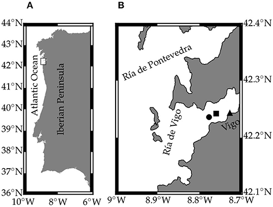
Figure 1. Map of the study area showing (A) the Iberian Peninsula and (B) the Ría de Vigo B). The circle indicates the EF sampling station (8.778°W 42.235°N), the square the ADCP position (8.761°W 42.241°N) and the triangle the Porto station (8.728°W 42.242°N).
2.2. Hydrography and Turbulence
Hydrographic and turbulent data were collected with a microstructure turbulence profiler MSS90 (Prandke and Stips, 1998). The profiler was equipped with two microstructure shear sensors (type PNS06), a microstructure temperature sensor (FP07), a high-precision CTD (Conductivity-Temperature-Depth) probe, a fluorescence sensor, and an accelerometer. On each sampling day, 10 profiles were conducted and then averaged. The profiler was balanced to have negative buoyancy in the water column and a sinking velocity in the range 0.4–0.7 ms−1.
Dissipation rates of turbulent kinetic energy (ϵ) were computed in 512 data point segments, with 50% overlap, from the vertical shear (∂zu) variance using the Taylor (1935) equation assuming isotropic turbulence:
where ν is the kinematic viscosity of seawater and 〈〉 denotes the ensemble average. The shear variance was computed by integrating the shear power spectrum. The lower integration limit was set to 2 cpm. The upper cut-off wavenumber for the integration of the shear spectrum was set as the Kolmogoroff number . An iterative procedure was applied to determine kc. The maximum upper cut-off was not allowed to exceed 30 cpm to avoid the noisy part of the spectrum. Assuming a universal form of the shear spectrum, ϵ was corrected for the loss of variance below and above the integration limits, using the polynomial functions reported by Prandke et al. (2000). ϵ values were then averaged in 1 m bins. Peaks due to particle collisions were removed by comparing the dissipation computed simultaneously from the two shear sensors. The turbulent diffusivity K was estimated from the Osborn (1980) formula:
where N2 is the squared buoyancy frequency and γ is the mixing efficiency, here considered to be 0.2 (Oakey, 1982). Although a growing body of evidence suggests that γ is not always constant, we follow the recommendation of Gregg et al. (2018) to use γ = 0.2 for microstructure studies until observations, laboratory experiments, and numerical simulations converge on a more accurate formulation. Furthermore, the Ría de Vigo is a system characterized by being marginally unstable to shear-driven turbulence (Fernández-Castro et al., 2018), which justifies the choice of this γ value (Smyth, 2020).
The mixed-layer depth (MLD) was determined as the depth where an increase of 0.125 kg m−3 was observed with respect to the surface values (~2 m). The turbulent layer depth (TLD) was computed using one-dimensional lagrangian simulations forced with the observed diffusivity profiles (Ross and Sharples, 2004). The new particle depth (zn+1) was computed in based of the present depth (zn) after:
where R ∈ [−1, 1] is a random number of variance and Δt the time-step chosen by ensuring that it was much lower than the minimum value of . In these simulations, 1,000 particles were released at the surface and let evolve in the diffusivity field for 24 h. The TLD was defined as the lower limit of the depth range containing 95% of 1,000 particles at the end of the simulation. The light availability was computed as the daily-average surface PAR in the turbulent layer computed following the expression reported in (Vallina and Simó, 2007):
where κ is the light attenuation coefficient determined from PAR profiles obtained with a Licor PAR sensor on each sampling day.
2.3. Current Velocities
The RD Instruments Acoustic Doppler Current Profiler (ADCP) was bottom-moored in the central part of the Ría de Vigo close to the EF station (8.761oW 42.241oN, ~ 45 m depth, Figure 1). Profiles of current velocity were acquired continuously from 3 March 2017 to 29 May 2018. A gap in data collection occurred from 30 May 2017 to 8 June 2017 due to maintenance operations. The measurements were made in 89 layers with a bin thickness of 0.5 m and the first bin located at 2 m above the ADCP transducers. Every 10 min, 85 samples of 3D currents were acquired at 2 Hz, averaged in ensemble and recorded. Resulting zonal and meridional velocity vector components were projected into the axis along the main channel (35o north of east) of the Ría de Vigo. Hence, the along-Ría component was positive into the Ría. Finally, these time-series were smoothed with the operator (Godin, 1972), which applies three consecutive moving averages with window size of 24, 24, and 25 h, with the aim of filtering out the tidal and supertidal frequencies. The residual current velocity along the main axis of the Ría at 32 m depth (u32) was selected to characterize the deep circulation in the Ría. Positive (negative) values indicate the deep water inflow (outflow) into the Ría and surface water outflow (inflow), corresponding to upwelling and downwelling conditions, respectively.
2.4. Inorganic Nutrients Concentration
Samples for the determination of dissolved inorganic nutrients (nitrate, nitrite, ammonium, phosphate, and silica) were collected from 8 to 9 depths, in the water column by using 5 l Niskin bottles. Samples were frozen at −20oC until further determination at the laboratory, following the methods described by Hansen and Koroleff (2007).
2.5. Nutrient Supply
Nutrient input into the surface layer of the Rías occurs mainly by coastal upwelling, while continental runoff and precipitation (Fernández et al., 2016) and turbulent diffusion (Moreira-Coello et al., 2017) represent minor inputs. An estimate of the supply of nitrate due to upwelling pulses was computed as the nitrate vertical advection induced by convergence of upwelled waters inside the Ría:
where l and A are the length of the mouth and surface area of the Ría (~10 km and ~174 km2, respectively), and is the nitrate concentration at the deepest sampling depth around 40 m depth. UI is the upwelling index averaged over the 3 days prior each sampling (Gilcoto et al., 2017). A null value was assigned to those samplings under downwelling conditions.
2.6. Chlorophyll a Concentration and Primary Production Rates
Chlorophyll a concentration (Chl a) and primary production rates were determined from samples collected at surface (~0.5–1 m) and 10 m depth. For the determination of total Chl a, 250 ml of seawater were filtered through polycarbonate filters of 0.2 μm, which were later frozen at −20oC until analysis. The fluorescence (Fluo) emitted by the Chl a was measured from pigments extracted in 90% acetone at 4oC overnight using a Turner designs Trilogy fluorometer previously calibrated with pure Chl a. The measured Chl a concentrations were used to calibrate the MSS fluorometer by using a linear regression (Chl a = 1.47 × Fluo−0.16, R2 = 0.89, n = 22) for Chl a concentration ranging between 0.26 and 5.83 mg m−3.
Primary production rates were determined by running incubations with the radioisotope 14C as described in Cermeño et al. (2016). Briefly, four 72 ml acid-washed polystyrene bottles (three light and one dark bottle) were filled with seawater from each depth. Each bottle was inoculated with ~ 5 μCi of and then incubated for 2 h starting at noon. An incubator equipped with a set of blue and neutral density plastic filters was used to simulate irradiance conditions at the original sampling depths. Temperature conditions during the incubation period were kept similar to those observed at surface (±1.5oC) by employing a closed refrigerated water system. Immediately after incubation, samples were filtered through 0.2 μm polycarbonate filters under low-vacuum pressure. Non-assimilated radioactive inorganic carbon retained in the filters was removed by exposing them to concentrated HCl fumes overnight. Radioactivity signal on each sample was determined on a 1409-012 Wallac scintillation counter, which used an internal standard for quenching correction.
Growth rates (μ) were computed as the ratio primary production to phytoplankton biomass. Carbon phytoplankton biomass was estimated assuming the C:Chl a ratios for three hydrographic conditions in the Ría de Vigo: stratification (55 ± 13), winter mixing (54 ± 27) and upwelling (35 ± 18) at the same station (Cermeño et al., 2005). In our case 35 ± 18 was used for upwelling and 55 ± 30 for downwelling and transitional periods. Daily growth rates were computed from hourly values considering the number of light hours on the sampling day.
2.7. Wavelet Analysis
Time-series of phytoplankton growth rates and turbulent layer depth were analyzed with the wavelet transform, a technique in which the evolution of the times-series variance is analyzed at different frequencies. The contribution of variance at different times and periods was determined by the wavelet power spectrum (WPS), which was represented in the time-period plane, the periodogram (Cazelles et al., 2008). The finite length of time-series provokes discontinuities at their borders delimited by the cone of influence, in which the edge effects are negligible (Torrence and Compo, 1998). The relation of two time-series can be identified in time and period in terms of coherence (Γ2, Liu, 1994), from 0 to 1 due to a smoothing in both time and period following the recommendation of Torrence and Webster (1999). Peaks in the spectrum can be assumed to be a true feature with a certain confidence by using a test against an assumed background level (Torrence and Compo, 1998). In this case, the background was simulated with 1000 replicas of surrogate times-series by using a hidden Markov model (HMM), in which the short-term temporal correlation of the original time-series is preserved (Cazelles and Stone, 2003). The null hypothesis tested is that the original and surrogate time-series had same value distribution and short-term autocorrelation (Cazelles et al., 2014) with 95% confidence level.
To apply the wavelet transform, the time-series have to be spaced in a regular time interval (δt). Hence, phytoplankton growth rates and turbulent layer depth were linearly interpolated onto an equi-spatially time-grid with δt ≈ 8 d and N = 52 points. The comparison between times-series was ensured by using the standardization of the variables, so they had nil mean and unit variance. An specific code was built on Python in order to conduct the wavelet analysis.
3. Results
3.1. Environmental and Hydrographic Conditions
The temporal variability of the smoothed (fortnight moving average) upwelling index and the smoothed current velocity sampled at 32 m depth allowed us to establish upwelling, downwelling, or transitional periods (Figure 2). Based on the bidirectional circulation of the Ría de Vigo, positive values of UI and deep current velocity correspond with the input of deep water, and negative values with the output of deep water. From sampling 1 to 11 (9 Mar 2017–18 May 2018) a spring transitional period (T1) was sampled characterized by the alternation of relatively short upwelling and downwelling events, which resulted in low averaged upwelling index of UI = 0.3 ± 0.1 m2s−1 (mean ± standard uncertainty of the mean, Table 1). Samplings 12–26 (25 May 2017 to 14 Sep 2017), when the averaged upwelling index was positive (UI = 1.7 ± 0.1 m2s−1), were characterized by spring-summer upwelling conditions (U1). Samplings 27–36 (21 Sep 2017–21 Nov 2017) recorded a fall transitional period (T2), with alternation of upwelling and downwelling events and null averaged upwelling index (UI = 0.0 ± 0.1 m2s−1). Between late fall and early spring (samplings 34–47, 30 Nov 2017–27 Mar 2018), downwelling conditions were dominant (D) and averaged upwelling index was negative (UI = −1.1 ± 0.1 m2s−1). Finally, in spring 2018 (samplings 48–52, 12 Apr 2018–10 May 2018) the beginning of the spring upwelling season (U2) was sampled, characterized by a mean upwelling index (UI = 1.9 ± 0.4 m2s−1) similar to the previous upwelling period (U1).
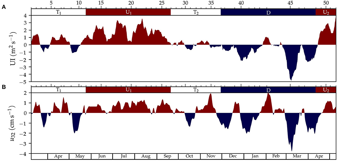
Figure 2. Time-series of fortnight moving average of (A) the upwelling index (UI) and (B) along-Ría residual current velocity at 32 meters depth (u32). The sign of UI and u32 is marked with red color for positive values (upwelling, deep flow into the Ría) and blue for negative (downwelling, deep flow out of the Ría). The ticks and numbers on the top axis indicate the sampling number and the colors, the periods for upwelling (U1 and U2, in red), downwelling (D, in blue), and transition (T1 and T2, in white).
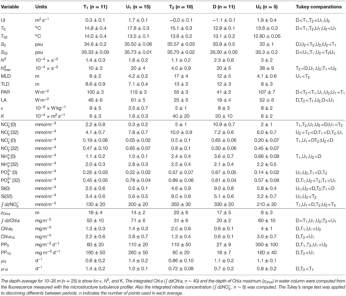
Table 1. Mean ± standard uncertainty of the mean for selected variables averaged on each time periods.
The variability in hydrographic properties sampled by the microstructure turbulence profiler is shown in Figures 3A–F and Table 1. The spring transitional period T1 (March–May 2017) was characterized by relatively low (14–15oC) and vertically homogeneous temperature. In general, salinity was relatively low at the surface (34.6 ± 0.2), which caused intermediate values of the mean squared buoyancy frequency (N2, 1.4 ± 0.3 × 10⁻⁴ s−2). Averaged dissipation rates (ϵ) in the water column were relatively large (9 ± 5 × 10⁻⁸ Wkg−1), which combined with intermediate N2 values caused intermediate values of averaged diffusivity (K, 6 ± 3 × 10⁻⁴ m2s−1). During the spring-summer upwelling period U1 (May–September 2017), surface temperature was relatively high whereas salinity was rather homogeneous in the water column. The thermal vertical gradient resulted in intermediate N2 values (1.8 ± 0.2 × 10⁻⁴ s−2), whereas ϵ (3.5 ± 0.7 × 10⁻⁸ Wkg−1) and K (1.6 ± 0.3 × 10⁻⁴ m2s−1) were comparatively low. The fall transitional period T2 (September–November 2017) was characterized by a decrease in surface temperature (15.1 ± 0.3oC), and relatively homogeneous vertical salinity distribution (35.57–35.70). The weak thermal stratification caused low N2 values (1.1 ± 0.2 × 10⁻⁴ s−2). Dissipation rates were relatively low (5 ± 1 × 10⁻⁸ Wkg−1), but the low N2 values provoked the highest values of K (40 ± 20 × 10−4 m2s−1). This increase was mainly due to the high values computed at depths greater than ~20 m in sampling 31 (18 Oct 2017, K = 146 × 10−4 m2s−1), and above ~30 m in sampling 36 (21 Nov 2017, K = 191 × 10−4 m2s−1). During the winter downwelling period D (December 2017–March 2018), low surface temperature (12.9 ± 0.1oC) and surface salinity (33.9 ± 0.5) were registered. This period was characterized by intense haline vertical stratification, which caused high N2 values (2.3 ± 0.8 × 10⁻⁴ s−2). Dissipation rates were relatively high (8 ± 3 × 10⁻⁸ Wkg−1), giving rise to high K (20 ± 10 × 10−4 m2s−1). During this period, high K values were calculated throughout the water column in sampling 38 (5 Dec 2017, K = 150 × 10−4 m2s−1). The spring 2018 upwelling period U2 (March–May 2018) presented low surface temperature (13.8 ± 0.3oC) and surface salinity (33 ± 1). The thermal, and specially, the haline vertical gradients, caused high N2 values (3 ± 2 × 10⁻⁴ s−2). Dissipation rates were relatively high (9 ± 2 × 10⁻⁸ Wkg−1), which, combined with the high N2 values, yielded intermediate K values (6 ± 2 × 10⁻⁴ m2s−1).
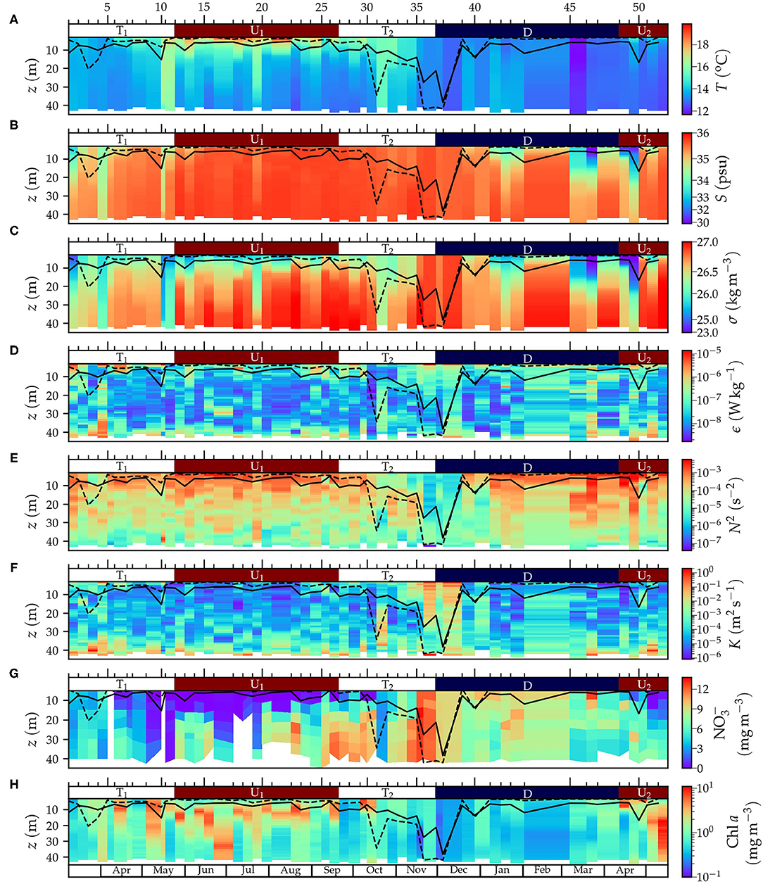
Figure 3. Time-series of the vertical distribution of (A) temperature (T), (B) salinity (S), (C) density anomaly (σ), (D) turbulent kinetic energy dissipation rate (ϵ), (E) squared buoyancy frequency (N2), (F) turbulent diffusivity (K), (G) nitrate concentration (), and (H) Chl a concentration. (A–F,H) Derived from data obtained from the microstructure profiler and (G) from water samples collected from the Niskin bottles. The solid and dashed black line denote the turbulent layer and mixed-layed depth, respectively. The ticks and numbers on the top axis indicate the sampling number and the colors, the periods for upwelling (U1 and U2, in red), downwelling (D, in blue), and transition (T1 and T2, in white).
The turbulent layer depth (TLD), an indication of the depth reached by currently active mixing (Brainerd and Gregg, 1995) computed by simulations forced with K profiles (see section 2), was significantly correlated with the mixed-layer depth (TLD = 0.48 × MLD + 5.4, R2 = 0.66, p < 0.001, n = 52), and exhibited similar seasonal variability (Figure 3). As a result of the enhanced K during samplings 36 and 38, maximum TLD values were computed during the fall transitional T2 (13 ± 2 m) and winter downwelling D (12 ± 3 m) periods, whereas TLD was shallower during the spring-summer upwelling U1 (7.1 ± 0.4 m). Most observations (n = 40) corresponded to shallow (< 9 m) MLD coinciding with slightly deeper (3-4 m) TLD. This could be the result of the limited number of microstructure turbulence data near the surface used for the calculation of both TLD and MLD. For samplings showing relatively deep mixed-layers (MLD > 9 m, n = 12), TLD was 8 ± 2 m shallower than MLD in average. In fact, in four sampling days, TLD was at least 12 m shallower than MLD (samplings 3, 31, 36, and 37), which suggests the occurrence of mixed-layers that were not actively mixing at the time of sampling.
3.2. Inorganic Nutrients
The temporal variability of the vertical distribution of nitrate is shown in Figure 3G and Table 1. During the spring transitional period T1, nitrate concentrations in surface (2.2 ± 0.8 μM) and deep waters (4.1 ± 0.7 μM) were relatively low. Nitrate concentration increased on average during the spring-summer upwelling U1 at deep waters (7.8 ± 0.7 μM), whereas lower concentrations were found at the surface (0.3 ± 0.2 μM). The fall transitional period T2 was characterized by increasing nitrate concentrations both at surface (5 ± 1 μM) and deep waters (10.0 ± 0.9 μM). Nitrate concentration increased during the winter downwelling D at the surface (10.9 ± 0.7 μM) but it decreased in deep layers (7.2 ± 0.6 μM). Finally, the spring upwelling U2 was characterized by declining nitrate concentrations at surface (2 ± 1 μM) and deep layers (6.0 ± 0.7 μM). Distinctive patterns in nitrate distribution were observed in samplings characterized by enhanced K (samplings 36 and 38). During these samplings, enhanced nitrate concentrations (≥ 9 μM) were sampled throughout the water column, coinciding with fall upwelling conditions.
Additional information about the vertical distribution of nitrite, ammonium, phosphate and silicate is shown in Supplementary Figure 1. In general, the seasonal variability of nitrite, phosphate and silicate concentration were very similar to the described nitrate distribution. In fact, a statistically significant positive relationship was found between nitrate and nitrite (, R2 = 0.56, p < 0.001, n = 428), phosphate (, R2 = 0.74, p < 0.001, n = 428) and silicate (, R2 = 0.73, p < 0.001, n = 428). However, no statistically significant relationship was found between nitrate and ammonium concentration (R2 = 0.11, p < 0.001, n = 428). Surface waters exhibited higher averaged ammonium concentration during winter downwelling during winter donwnwelling (3.6 ± 0.7 μM), whereas during the other periods values ranged between 0.66 ± 0.08 μM (U2) and 2.4 ± 0.4 μM (T2). The seasonal variability of ammonium concentrations at deep waters was low (2.0–2.8μM).
3.3. Chlorophyll a, Primary Production and Phytoplankton Growth Rates
The temporal and vertical distribution of Chl a concentration, determined from the calibrated fluorescence sensor included in the microstructure turbulence profiler, is shown in Figure 3H. Relatively large short-term variability was observed for the depth of the Chl a maximum, which was shallower and less variable during the upwelling periods (14 ± 2 m during U1 and 8 ± 3 m during U2) than the transitional T1 and T2 and the downwelling period (18 ± 4, 20 ± 3, and 17 ± 5 m, respectively). Higher values of depth-integrated Chl a were measured for the spring-summer upwelling U1 (71 ± 6 mgm−2) and U2 (60 ± 10 mgm−2) periods, whereas lower values were observed during winter downwelling D (20 ± 2 mgm−2).
The temporal variability of Chl a concentration, primary production rates and phytoplankton growth rates determined at the surface and 10 m depth from water samples collected from Niskin bottles are shown in Figure 4. All these variables exhibited a distinct seasonal variability, which allowed fitting the data to a sinusoidal curve to highlight the seasonal cycle. The amplitude of the seasonal variability for Chl a and primary production was larger at 10 m. In agreement with the chlorophyll-derived fluorescence data from the microstructure profiler, maximum values of extracted Chl a and primary production were measured during spring-summer upwelling, whereas minimum values were obtained mainly during winter downwelling. On average, Chl a and primary production were lower at the surface than at 10 m depth during the spring transition T1 and spring-summer upwelling U1, whereas the opposite pattern was found during the fall transition T2, the winter downwelling and the spring upwelling U2.
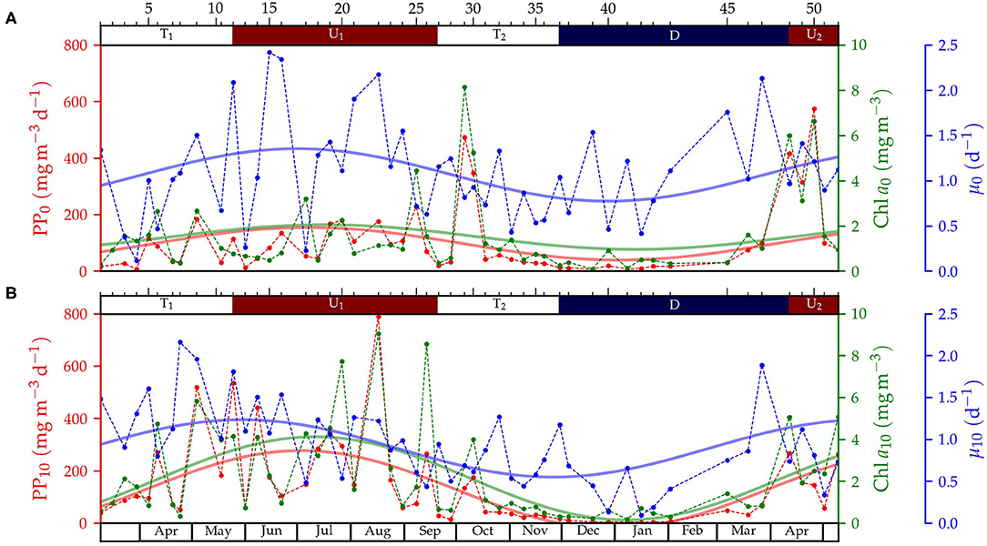
Figure 4. Time-series of primary production rates (PP, red), chlorophyll a (Chl a, green) and growth rates (μ, blue) at (A) surface (z ~ 0m) and (B) 10 m depth. Data for each sampling are represented by circles connected by a dashed line, and the seasonal mode (computed by fitting to a sinusoidal curve), with solid line. The ticks and numbers on the top axis indicate the sampling number and the colors, the periods for upwelling (U1 and U2, in red), downwelling (D, in blue), and transition (T1 and T2, in white).
As the result of the observed variability, phytoplankton growth rates were in general higher at the surface than at 10 meters depth. On average, surface rates were higher during spring-summer upwelling U1 (1.4 ± 0.2 d−1), downwelling (1.1 ± 0.2 d−1) and spring upwelling U2 (1.1 ± 0.1 d−1), whereas lower rates were computed during transitional periods T1 (0.8 ± 0.2 d−1) and T2 (0.9 ± 0.1 d−1). At 10 m, growth rates were higher during the spring transitional period T1 (1.4 ± 0.2 d−1) and spring-summer upwelling U1 (1.0 ± 0.1 d−1), whereas lower values were computed for the transitional T2 (0.72 ± 0.08 d−1) and downwelling period (0.7 ± 0.2 d−1). Since higher phytoplankton growth rates were estimated at the surface layer and a similar seasonal pattern was observed at the two sampling depths, we focus on surface rates to investigate the relationship between phytoplankton growth and mixing.
3.4. Relationship Between Turbulent Mixing and Phytoplankton Growth
We first investigated the relationship between turbulent mixing and surface phytoplankton growth rate over seasonal scales by plotting the variability of the TLD and phytoplankton growth in Figure 5. The annual mode, computed for both variables by fitting the observations to a sinusoidal curve, showed that in general maximum growth rates coincided with shallow turbulent layers, whereas minimum values corresponded to deep turbulent layers. Similarly, high phytoplankton growth was coincident with periods of high values of the light and nitrate availability indices, and vice versa.
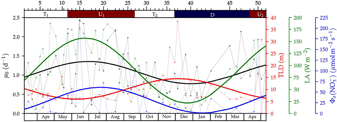
Figure 5. Time-series of surface phytoplankton growth rates (μ0, black), turbulent layer depth (TLD, red), light availability (LA, green) and nitrate advective flux [, blue]. Data for each sampling is represented by circles connected by a dashed line, and the seasonal mode (computed by fitting to a sinusoidal function), with a solid line. The ticks and numbers at the top axis indicate the sampling number and the colors, the periods for upwelling (U1 and U2, in red), downwelling (D, in blue), and transition (T1 and T2, in white).
In addition to the seasonal mode described above, Figure 5 evidenced the existence of short-term variability both in TLD and phytoplankton growth. In fact, 44 and 60% of the variance of TLD and surface growth rates, respectively, were distributed in periods shorter than 128 d. The wavelet analysis, used to investigate this shorter-term variability (Figure 6), showed that TLD variance was larger during the fall transition T2 and winter downwelling through all the periods with maxima at 34 and 91 days (Figure 6A). The variance of surface growth rates displayed two main components extending mostly during the spring-summer upwelling U1 centered at 26 and 56 days (Figure 6B). Growth rates at 10 m (Supplementary Figure 2A) exhibited variance maxima during the spring transition T1 (centered at 25 days), and during the fall transition T2 and winter downwelling (109 days period).
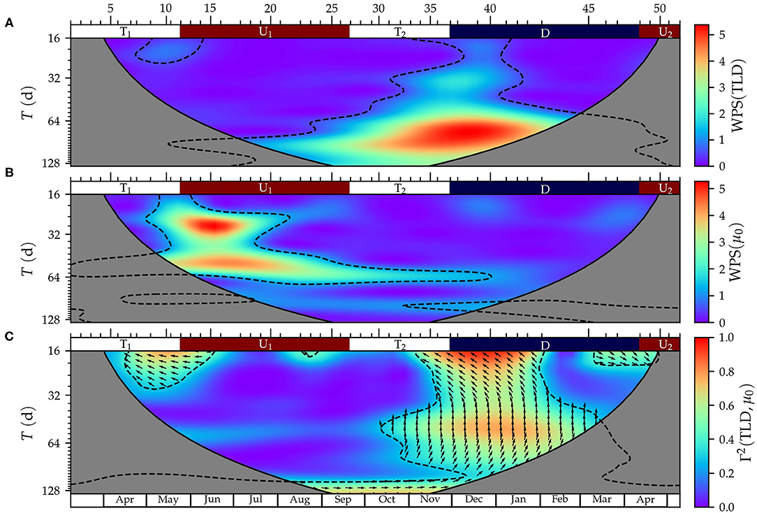
Figure 6. Wavelet analysis of turbulent layer depth (TLD) and surface phytoplankton growth rates (μ0). (A) Wavelet power spectrum (WPS) of TLD, (B) WPS of μ0, and (C) wavelet coherence (Γ2) and phase difference (δϕ) between TLD and μ0. The solid black line indicates the cone of influence inside which the edge effects have no influence. The black dashed lines denote the 0.05 significance regions. The arrows indicate δϕ measured with respect to the horizontal axis in the anti-clockwise direction; e.g., → for δϕ = 0o and ↑ for δϕ = 90o. For simplicity, arrows are only plotted inside the regions where significance was higher than 0.05 and only one arrow is plotted every eight period-points. The ticks and numbers at the top axis indicate the sampling number and the colors, the periods for upwelling (U1 and U2, in red), downwelling (D, in blue), and transition (T1 and T2, in white).
The relationship between the variance in TLD and surface phytoplankton growth rates was investigated via the coherence (Γ2) computed using the wavelet analysis (Figure 6C). Also, the phase difference (δφ) between both signals was calculated to characterize the delay between the two time-series. The variables are in phase (δφ = 0o) when their maxima coincide in time, whereas they are in phase opposition (δφ = 180o) when the maximum of one variable coincides with the minimum of the other, and vice versa. TLD and surface growth rates showed significant coherence during the end of the spring transitional T1 and the beginning of the spring-summer upwelling U1 (~16–30 d period) and from the end of the fall transitional period T2 to the middle of the winter downwelling (~16–90 d periods). The highest coherence (Γ2 > 0.8) occurred for periods ~16–20 d, for which the averaged phase difference was 145 ± 4o. The coherence between TLD and growth rates at 10 m depth (Supplementary Figure 2B) was significant during the end of the spring transitional T1 and the beginning of the spring-summer upwelling U1(~16–56 d period) and from the fall transitional period T2 to the spring upwelling U2 with maximum values at ~16 and ~35 d.
4. Discussion
As far as we know this study represents the first attempt to investigate the relationship between mixing and phytoplankton growth, by using coincident observations of microstructure turbulence and phytoplankton growth, in a coastal upwelling system. In general, higher turbulent mixing was observed during fall-winter transitional and downwelling periods, whereas weaker mixing corresponded to spring-summer transition and upwelling. However, this pattern was mainly driven by the enhanced turbulent diffusivity quantified during two samplings (36 and 38 sampled on 21 November 2017 and 5 December 2017, respectively). This increase in diffusivity was mainly due to a decrease in the buoyancy frequency, as the consequence of the weak vertical gradient observed in both temperature and salinity. According to the analysis of hydrographic and current velocity data, these two samplings were under the influence of fall upwelling conditions. Although this system is characterized by predominant upwelling conditions during the spring and summer (Fraga, 1981), previous studies described the existence of an important short-term variability in wind conditions, which generates a succession of upwelling-downwelling episodes in periods of 15 days (Álvarez-Salgado et al., 1993; Nogueira et al., 1997; Figueiras et al., 2002). Recently, using direct observations of currents, the mean duration of these upwelling-downwelling episodes has been estimated in ~ 3 days (Gilcoto et al., 2017). The vertical homogenization of the thermohaline conditions, due to the advection of salty oceanic waters inside the Rías, during fall upwelling events erodes the frequent haline stratification driven by increasing precipitation and runoff (Rosón et al., 2008), and enhances mixing.
The seasonality of turbulent mixing in the upper ocean, both in coastal and open-ocean regions, remains poorly assessed due to the limited number of microstructure observations spanning entire annual cycles, such that the limited present knowledge derived mostly from indirect methods (Whalen et al., 2012; Warner et al., 2016; Inoue et al., 2017; Evans et al., 2018; Thakur et al., 2019; Cherian et al., 2020). Previous studies carried out in this region provided information about the variability of turbulent diffusivity on short-time scales during specific seasons (Barton et al., 2016; Villamaña et al., 2017; Fernández-Castro et al., 2018; Broullón et al., 2020) or along seasonal scales with coarser temporal resolution (Cermeño et al., 2016; Moreira-Coello et al., 2017).
Our results show that surface growth rates, which ranged from 0.11 to 2.42 d−1 (0.008–0.226 h−1), were in general higher during spring-summer transitional and upwelling periods, and minimum during fall-winter transitional and downwelling. These values are consistent with previous estimates determined for this system, by using a similar methodology, but with coarser temporal resolution. An early study carried out in the Ría de Arousa during an upwelling event (Hanson et al., 1986), reported depth-averaged phytoplankton growth rates ranging from < 0.1 to 1.89 d−1 (from < 0.004 to 0.0788 h−1). Cermeño et al. (2016) estimated slightly lower phytoplankton growth rates at the same station in the Ría de Vigo (~0.004–0.114 h−1). Our data, derived from short (2 h) incubations experiments, are also consistent with apparent phytoplankton growth rates estimated from the dilution technique which ranged from 0.31 to 1.75 d−1 (Teixeira and Figueiras, 2009). However, maybe due to aliasing of short-term variability in their coarser observations, previous studies in the region did not report a clear seasonal cycle in phytoplankton growth rates. Seasonal trends in phytoplankton growth, consistent with our findings, have been described in several studies carried out in contrasting regions, mainly by using the dilution technique (Kim et al., 2007; Gutiérrez-Rodríguez et al., 2011; Lawrence and Menden-Deuer, 2012; Anderson and Harvey, 2019).
The temporal coverage and resolution of our study allowed interpreting our results within the conceptual framework of the Critical Turbulence Hypothesis (CTH, Huisman et al., 1999a,b, Figure 7A). According to the CTH, positive net phytoplankton growth will occur when (1) the water column depth is shallower than the critical depth, which is consistent with the Critical Depth Hypothesis (CDH, Sverdrup, 1953), or (2) when turbulent diffusivity in a mixed water column is lower than a critical value, which causes the timescale for phytoplankton growth to be less than the cell's residence time in the portion of the water column where net growth can be achieved. In this case, the depth of the turbulent layer would be shallower than the mixed layer depth.
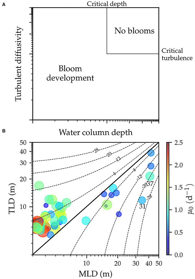
Figure 7. Theoretical framework of the Critical Turbulence Hypothesis (CTH). (A) Adaptation of original diagram (Figure 2 in Huisman et al., 1999a) where critical conditions of the water column depth and turbulent diffusivity for phytoplankton bloom formation are indicated. Critical values must be interpreted for visual purposes as an approximation. (B) Phytoplankton surface growth rates (μ0) vs. the mixed-layer depth (MLD) and the turbulent layer depth (TLD). The curve of constant differences between TLD and MLD of ±4, ±12, ±20, and ±28 are represented by a dotted line and of 0 (1:1 line) by a solid line. Logarithmic scales are used in both axes.
Huisman et al. (1999a) described these two distinct and independent mechanisms by using simulations with variable turbulent diffusivity and water column depth. Similar to the CDH, they assumed that phytoplankton growth was only limited by light, and also constant values in time and depth for turbulence diffusivity and the phytoplankton loss term. In order to interpret our results under this theoretical framework, we performed some modifications on the original diagram (Figure 7A). First, we used the mixed-layer depth instead of the water column depth, to indicate the depth of the water column where density was relatively vertically homogeneous. Second, we used the turbulent layer depth, instead of turbulent diffusivity, to consider both the magnitude and the vertical structure of turbulent mixing. Finally, we used surface growth rate instead of depth-integrated phytoplankton growth rates to represent phytoplankton growth in the turbulent layer (Figure 7B). Consequently, phytoplankton growth was always positive and its variability must be interpreted in relative terms instead of positive or negative growth, as in the original diagram.
In agreement with the first scenario proposed by the CTH, our results showed that higher phytoplankton growth rates were found for periods of shallow turbulent and mixed-layers during spring-summer transitional and upwelling periods, whereas low values were observed during periods of deep turbulent and mixed-layers (fall-winter transitional and downwelling periods). Unfortunately, our dataset was not suitable to assess the second scenario described by Huisman et al. (1999a), as most observations corresponded to shallow mixed- and turbulent layers. Only two samplings (31 and 37) showed the mixed-layer to be much deeper (~20 m) than the turbulent layer, suggesting that the mixed-layer was not actively mixing in <1 day. The surface phytoplankton growth rate for sampling 31, 2 days after the passage of Hurricane Ophelia, was relatively low (0.73 d−1), whereas this rate was slightly higher during sampling 37 (1.0 d−1).
Due to the difficulty to quantify turbulence in the field, previous studies using the CTH theoretical framework mainly used hydrographic and atmospheric data to infer mixing conditions in the upper layer, and its relationship with phytoplankton growth in different regions as the North Atlantic (Chiswell, 2011; Chiswell et al., 2013; Mignot et al., 2018), the North West European Shelf (Wihsgott et al., 2019), the southwest Pacific (Chiswell, 2011; Chiswell et al., 2013), the Western Mediterranean Sea (Bernardello et al., 2012; Kessouri et al., 2018), the Chukchi Sea (Lowry et al., 2018), and the Labrador Sea (Marchese et al., 2019). The decrease in turbulence that could explain the TLD being shallower than the MLD (second scenario proposed for the CTH) has been associated with a reduction in air-sea fluxes that generally precedes mixed-layer shoaling at the end of winter (Taylor and Ferrari, 2011) and lowered wind stress (Chiswell, 2011; Chiswell et al., 2013). Moreover, Brody and Lozier (2014) proposed that the mixing-length scale of the largest energy-containing eddies in the upper ocean is a better predictor for bloom initiation than the decrease in mixed-layer depth, the onset of positive heat fluxes, or the decrease in wind strength. They also found that the shift from buoyancy-driven to wind-driven mixing in late winter creates the decrease in mixing length scale, and thus the conditions necessary for blooms to begin (Brody and Lozier, 2015).
Only a limited number of studies have previously used microstructure observations to investigate the relationship between turbulence and phytoplankton activity and composition. Among those, most studies were focused on analyzing the role of mixing and nutrient supply as drivers of phytoplankton community structure (Sharples et al., 2007, 2009; Machado et al., 2014; Villamaña et al., 2017, 2019). As far as we know only two studies have used microturbulence observations to investigate phytoplankton growth under the CTH framework. Huisman et al. (2004) extended the CTH including competition theory, to predict how changes in turbulent mixing affect competition for light between buoyant and sinking phytoplankton species. Consistent with the model prediction, results from a lake experiment showed that changes in turbulent mixing caused a dramatic shift in phytoplankton species composition. In coherence with the CTH, Hopkins et al. (2021) used a relatively short (2 weeks) period of high-frequency (sub-hourly) observations collected from gliders in the Northwest European Shelf to conclude that turbulent mixing, that mediate light availability, was the key process governing phytoplankton growth in spring.
Our study covers a full annual cycle which allows investigating the coupling between turbulent mixing and phytoplankton growth at different temporal scales. Our results show that shallower mixed- and turbulent layers conditions were not enough to ensure phytoplankton growth, as low phytoplankton growth was also found under these circumstances. It is important to note that, instead of following a single phytoplankton bloom over time, our weekly approach involves sampling different blooms at different stages of development. Previous studies in this region have described that the spring-summer and fall phytoplankton growth seasons are the result of a succession of blooms triggered by the short-term variability in the upwelling regime and runoff water pulses (Nogueira and Figueiras, 2005). This is consistent with observations carried out in the North Atlantic where fluctuations in the winter mixed-layer depth triggered occasional short-live blooms (Mignot et al., 2018). Using a wavelet transform analysis we showed that the coupling between turbulent mixing and phytoplankton growth in this system occurs not only over the seasonal cycle, but also at shorter temporal scales. These results suggest that mixing could act as a control factor on phytoplankton growth over the seasonal cycle, but also being involved in the formation of occasional short-lived phytoplankton blooms.
5. Conclusions
By analyzing a unique dataset combining weekly observations of microstructure turbulence and phytoplankton growth collected in the NW Iberian coastal upwelling we show that coupling between turbulent mixing and phytoplankton growth occurs over the seasonal cycle, but also at shorter temporal scales. In agreement with the Critical Turbulence Hypothesis (Huisman et al., 1999a,b), our results indicate that higher values of phytoplankton growth occurred during spring-summer transitional and upwelling periods, when the depth of the turbulent layer was shallower, whereas the opposite pattern was observed during fall-winter transitional and downwelling periods. However, shallower turbulent layers were not enough to stimulate phytoplankton growth, as low growth rates were observed during the same conditions. Despite our unprecedented sampling effort, we are aware that a significant part of the variability in this system was still not captured, which deterred us from unveiling the mechanisms driving the coupling between mixing and phytoplankton growth rates, specially at short time-scales. Furthermore, longer observations will be needed to discern whether the seasonal patterns described here are characteristic of the study system or determined by the specific investigated sampling period.
The Critical Turbulence Hypothesis assumes that phytoplankton growth is exclusively limited by light and that the phytoplankton loss rate is independent of depth and constant through time. However, mixing conditions in the water column influence light but also nutrient availability for phytoplankton cells. Our results indicate that, in general, higher phytoplankton growth occurs when light but also nitrate availability was higher. Although our study was performed in a nutrient-rich coastal upwelling ecosystem, previous studies in the region have shown that phytoplankton is limited by nitrogen during the summer, or at least it positively responds to its addition (Martínez-García et al., 2010). Moreover, although phytoplankton blooms have traditionally been attributed to changes in “bottom-up” environmental factors controlling phytoplankton division rates, such as light and nutrients (e.g., Hunter-Cevera et al., 2016; Wihsgott et al., 2019), changes in phytoplankton biomass are the result of the interplay between phytoplankton division rates and the sum of all loss terms. Recent studies using satellite, in situ observations and modeling approaches highlighted the relevance of variability in loss rates (Behrenfeld, 2010; Boss and Behrenfeld, 2010; Behrenfeld et al., 2013). The Disturbance Recovery Hypothesis proposed by Behrenfeld and Boss (2014) argues that, contrary to the CDH, bloom initiation takes place in the winter because deep mixing dilutes phytoplankton cell density, thus reducing the encounter rate between predator and prey. It is important to note that our phytoplankton growth estimates, as derived from short carbon uptake experiments, are close to gross rates, and therefore do not reflect the balance between cell division and loss rates. Moreover, the time step we used for the wavelet analysis (8 days) is much longer than the time-scale for phytoplankton growth (~1 day). Future studies combing higher temporal resolution and longer observations, together with modeling approaches will be required in order to discern the mechanisms responsible for the coupling between mixing and phytoplankton growth observed in this system, and to evaluate the role of “bottom-up” and “top-down” control factors.
Despite their small surface extension (1% of the global ocean) eastern boundary upwelling systems account for 5% to the global marine primary production (Carr, 2001) and 20% of global fish catch (Chavez and Messié, 2009). One unresolved question is these regions is the regulation of primary production. Substantial variability in the ratio of nitrate supply to primary production has been described (Messié et al., 2009), indicating that regulators other than nitrate supply must be at play. In agreement with previous studies (Hardman-Mountford et al., 2003; Rossi et al., 2009; Fearon et al., 2020), our results indicate that turbulent mixing may control phytoplankton growth at the different time-scales involved in the physical-biological coupling in these systems.
Anthropogenic global change perturbations have the potential to affect phytoplankton dynamics, including the timing and magnitude of blooms (e.g., Hunter-Cevera et al., 2016; Jena and Narayana Pillai, 2020). Therefore, identifying the mechanisms responsible for the formation of phytoplankton blooms, including turbulent mixing (Károly et al., 2020), is key to understand the role of the ocean in the present and future climate.
Data Availability Statement
The original contributions presented in the study are included in the article/Supplementary Material, further inquiries can be directed to the corresponding author/s.
Author Contributions
AC, BM-C, and BF-C designed the overall study. PC, EF, AF-L, MG, MP-L, and BM-C carried out the observations and performed experiments in the lab. AC analyzed the dataset. AC, BM-C, and BF-C prepared the manuscript with contributions from all the co-authors. All authors contributed to the article and approved the submitted version.
Funding
This research was supported by grant CTM2016-75451-C2-1-R from the Spanish Ministry of Economy and Competitiveness to BM-C. AC was supported by a predoctoral fellowship for the doctoral formation (BES-2017-080935) from the Spanish Ministry of Economy and Competitiveness.
Conflict of Interest
The authors declare that the research was conducted in the absence of any commercial or financial relationships that could be construed as a potential conflict of interest.
Publisher's Note
All claims expressed in this article are solely those of the authors and do not necessarily represent those of their affiliated organizations, or those of the publisher, the editors and the reviewers. Any product that may be evaluated in this article, or claim that may be made by its manufacturer, is not guaranteed or endorsed by the publisher.
Acknowledgments
We thank the crew of the R/V Kraken and the R/V José María Navaz, and also all the scientists involved in data and water samples collection, for their valuable support during the sampling at sea.
Supplementary Material
The Supplementary Material for this article can be found online at: https://www.frontiersin.org/articles/10.3389/fmars.2021.712342/full#supplementary-material
References
Acuña, J. L., López-Alvarez, M., Nogueira, E., and González-Taboada, F. (2010). Diatom flotation at the onset of the spring phytoplankton bloom: an in situ experiment. Mar. Ecol. Prog. Ser. 400, 115–125. doi: 10.3354/meps08405
Álvarez-Salgado, X. A., Rosón, G., F. Pérez, F., Figueiras, F., and Ríos, A. (1996). Nitrogen cycling in an estuarine upwelling system, the Ría de Arousa (NW Spain). II. Spatial differences in the short-time-scale evolution of fluxes and net budgets. Mar. Ecol. Prog. Ser. 135, 275–288.
Álvarez-Salgado, X. A., Rosón, G., Pérez, F. F., and Pazos, Y. (1993). Hydrographic variability off the Rías Baixas (NW Spain) during the upwelling season. J. Geophys. Res. 98, 14447–14455. doi: 10.1029/93JC00458
Anderson, S. R., and Harvey, E. L. (2019). Seasonal variability and drivers of microzooplankton grazing and phytoplankton growth in a subtropical estuary. Front. Mar. Sci. 6:174. doi: 10.3389/fmars.2019.00174
Arteaga, L., Boss, E., Behrenfeld, M., Westberry, T., and Sarmiento, J. (2020). Seasonal modulation of phytoplankton biomass in the southern ocean. Nat. Commun. 11:5364. doi: 10.1038/s41467-020-19157-2
Backhaus, J., Wehde, H., Hegseth, E., and Kämpf, J. (1999). “Phyto-convection”: the role of oceanic convection in primary production. Mar. Ecol. Prog. Ser. 189, 77–92. doi: 10.3354/meps189077
Bakun, A. (1973). Coastal Upwelling Indices, West Coast of North America, 1946-71. Technical report, United States, Departament of Commerce, National Oceanic and Atmospheric Administration, National Marine Fisheries Service.
Barton, E. D., Torres, R., Figueiras, F. G., Gilcoto, M., and Largier, J. (2016). Surface water subduction during a downwelling event in a semienclosed bay. J. Geophys. Res. 121, 7088–7107. doi: 10.1002/2016JC011950
Behrenfeld, M. J. (2010). Abandoning Sverdrup's Critical Depth Hypothesis on phytoplankton blooms. Ecology 91, 977–989. doi: 10.1890/09-1207.1
Behrenfeld, M. J., and Boss, E. S. (2014). Resurrecting the ecological underpinnings of ocean plankton blooms. Annu. Rev. Mar. Sci. 6, 167–194. doi: 10.1146/annurev-marine-052913-021325
Behrenfeld, M. J., Doney, S. C., Lima, I., Boss, E. S., and Siegel, D. A. (2013). Annual cycles of ecological disturbance and recovery underlying the subarctic Atlantic spring plankton bloom. Glob. Biogeochem. Cycles 27, 526–540. doi: 10.1002/gbc.20050
Bernardello, R., Cardoso, J. G., Bahamon, N., Donis, D., Marinov, I., and Cruzado, A. (2012). Factors controlling interannual variability of vertical organic matter export and phytoplankton bloom dynamics-a numerical case-study for the NW Mediterranean Sea. Biogeosciences 9, 4233–4245. doi: 10.5194/bg-9-4233-2012
Boss, E., and Behrenfeld, M. (2010). In situ evaluation of the initiation of the North Atlantic phytoplankton bloom. Geophys. Res. Lett. 37, 1–5. doi: 10.1029/2010GL044174
Brainerd, K. E., and Gregg, M. C. (1995). Surface mixed and mixing layer depths. Deep Sea Res. Part I Oceanogr. Res. Pap. 42, 1521–1543.
Brody, S. R., and Lozier, M. S. (2014). Changes in dominant mixing length scales drive phytoplankton bloom initiation in the subpolar North Atlantic. Geophys. Res. Lett. 41, 3197–3203. doi: 10.1002/2014GL059707
Brody, S. R., and Lozier, M. S. (2015). Characterizing upper-ocean mixing and its effect on the spring phytoplankton bloom with in situ data. ICES J. Mar. Sci. 72, 1961–1970. doi: 10.1093/icesjms/fsv006
Brody, S. R., Lozier, M. S., and Dunne, J. P. (2013). A comparison of methods to determine phytoplankton bloom initiation. J. Geophys. Res. 118, 2345–2357. doi: 10.1002/jgrc.20167
Broullón, E., López-Mozos, M., Reguera, B., Chouciño, P., Dolores Doval, M., Fernández-Castro, B., et al. (2020). Thin layers of phytoplankton and harmful algae events in a coastal upwelling system. Prog. Oceanogr. 189:102449. doi: 10.1016/j.pocean.2020.102449
Carr, M.-E. (2001). Estimation of potential productivity in eastern boundary currents using remote sensing. Deep Sea Res. Part II Top. Stud. Oceanogr. 49, 59–80. doi: 10.1016/S0967-0645(01)00094-7
Cazelles, B., Cazelles, K., and Chavez, M. (2014). Wavelet analysis in ecology and epidemiology: impact of statistical tests. J. R. Soc. Interface 11:20130585. doi: 10.1098/rsif.2013.0585
Cazelles, B., Chavez, M., Berteaux, D., Ménard, F., Vik, J. O., Jenouvrier, S., and Stenseth, N. C. (2008). Wavelet analysis of ecological time series. Oecologia 156, 287–304. doi: 10.1007/s00442-008-0993-2
Cazelles, B., and Stone, L. (2003). Detection of imperfect population synchrony in an uncertain world. J. Anim. Ecol. 72, 953–968. doi: 10.1046/j.1365-2656.2003.00763.x
Cermeño, P., Chouciño, P., Fernández-Castro, B., Figueiras, F. G., Marañón, E., Marrasé, C., et al. (2016). Marine primary productivity is driven by a selection effect. Front. Mar. Sci. 3:173. doi: 10.3389/fmars.2016.00173
Cermeño, P., Marañón, E., Pérez, V., Serret, P., Fernández, E., and Castro, C. G. (2006). Phytoplankton size structure and primary production in a highly dynamic coastal ecosystem (Ría de Vigo, NW-Spain): seasonal and short-time scale variability. Estuar. Coast. Shelf Sci. 67, 251–266. doi: 10.1016/j.ecss.2005.11.027
Cermeño, P., Marañón, E., Rodríguez, J., and Fernández, E. (2005). Large-sized phytoplankton sustain higher carbon-specific photosynthesis than smaller cells in a coastal eutrophic ecosystem. Mar. Ecol. Prog. Ser. 297, 51–60. doi: 10.3354/meps297051
Chavez, F. P., and Messié, M. (2009). A comparison of eastern boundary upwelling ecosystems. Prog. Oceanogr. 83, 80–96. doi: 10.1016/j.pocean.2009.07.032
Cherian, D. A., Shroyer, E. L., Wijesekera, H. W., and Moum, J. N. (2020). The seasonal cycle of upper-ocean mixing at 8°n in the Bay of Bengal. J. Phys. Oceanogr. 50, 323–342. doi: 10.1175/JPO-D-19-0114.1
Chiswell, S. M. (2011). Annual cycles and spring blooms in phytoplankton: don't abandon Sverdrup completely. Mar. Ecol. Prog. Ser. 443, 39–50. doi: 10.3354/meps09453
Chiswell, S. M., Bradford-Grieve, J., Hadfield, M. G., and Kennan, S. C. (2013). Climatology of surface chlorophyll a, autumn-winter and spring blooms in the southwest Pacific Ocean. J. Geophys. Res. 118, 1003–1018. doi: 10.1002/jgrc.20088
Chiswell, S. M., Calil, P. H., and Boyd, P. W. (2015). Spring blooms and annual cycles of phytoplankton: a unified perspective. J. Plankton Res. 37, 500–508. doi: 10.1093/plankt/fbv021
Evans, D. G., Lucas, N. S., Hemsley, V., Frajka-Williams, E., Naveira Garabato, A. C., Martin, A., et al. (2018). Annual cycle of turbulent dissipation estimated from seagliders. Geophys. Res. Lett. 45, 10,560–10,569. doi: 10.1029/2018GL079966
Fearon, G., Herbette, S., Veitch, J., Cambon, G., Lucas, A. J., Lemarié, F., et al. (2020). Enhanced vertical mixing in coastal upwelling systems driven by diurnal-inertial resonance: numerical experiments. J. Geophys. Res. 125, 1–23. doi: 10.1029/2020JC016208
Fernández, E., Álvarez-Salgado, X. Á., Beiras, R., Ovejero, A., and Martínez, G. (2016). Coexistence of urban uses and shellfish production in an upwelling-driven, highly productive marine environment: the case of the ría de vigo (Galicia, Spain). Region. Stud. Mar. Sci. 8, 362–370. doi: 10.1016/j.rsma.2016.04.002
Fernández-Castro, B., Gilcoto, M., Naveira-Garabato, A. C., Villamaña, M., Graña, R., and Mouriño-Carballido, B. (2018). Modulation of the semidiurnal cycle of turbulent dissipation by wind-driven upwelling in a coastal embayment. J. Geophys. Res. 123, 4034–4054. doi: 10.1002/2017jc013582
Field, C., Behrenfeld, M., Randerson, J., and Falkowski, P. (1998). Primary production of the biosphere: Integrating terrestrial and oceanic components. Science 281, 237–240. doi: 10.1126/science.281.5374.237
Figueiras, F. G., Labarta, U., and Reiriz, M. J. F. (2002). Coastal Upwelling, Primary Production and Mussel Growth in the Rías Baixas of Galicia. Dordrecht: Springer Netherlands.
Fraga, F. (1981). Upwelling off the Galician coast, northwest Spain. Estuar. Sci. 1, 176–182. doi: 10.1029/CO001p0176
Franks, P. J. S. (2015). Has Sverdrup's critical depth hypothesis been tested? Mixed layers vs. turbulent layers. ICES J. Mar. Sci. 72, 1897–1907. doi: 10.1093/icesjms/fsu175
Fréon, P., Barange, M., and Arístegui, J. (2009). Eastern boundary upwelling ecosystems: integrative and comparative approaches. Prog. Oceanogr. 83, 1–14. doi: 10.1016/j.pocean.2009.08.001
Gilcoto, M., Largier, J. L., Barton, E. D., Piedracoba, S., Torres, R., Graña, R., et al. (2017). Rapid response to coastal upwelling in a semienclosed bay. Geophys. Res. Lett. 44, 2388–2397. doi: 10.1002/2016GL072416
Gomez-Gesteira, M., Moreira, C., Alvarez, I., and de Castro, M. (2006). Ekman transport along the Galician coast (Northwest Spain) calculated from forecasted winds. J. Geophys. Res. 111. doi: 10.1029/2005JC003331
Gregg, M. C., D'Asaro, E. A., Riley, J. J., and Kunze, E. (2018). Mixing efficiency in the ocean. Annu. Rev. Mar. Sci. 10, 443–473. doi: 10.1146/annurev-marine-121916-063643
Gutiérrez-Rodríguez, A., Latasa, M., Scharek, R., Massana, R., Vila, G., and Gasol, J. M. (2011). Growth and grazing rate dynamics of major phytoplankton groups in an oligotrophic coastal site. Estuar. Coast. Shelf Sci. 95, 77–87. doi: 10.1016/j.ecss.2011.08.008
Hansen, H. P., and Koroleff, F. (2007). “Determination of nutrients,” in Methods of Seawater Analysis eds K. Grasshoff, K. Kremling and M. Ehrhardt (Weinheim: Wiley-VCH Verlag GmbH), 159–228.
Hanson, R. B., Alvarez-Ossorio, M. T., Cal, R., Campos, M. J., Roman, M., Santiago, G., et al. (1986). Plankton response following a spring upwelling event in the Ria de Arosa, Spain. Mar. Ecol. -Prog. Ser. 32, 101–113.
Hardman-Mountford, N., Richardson, A., Agenbag, J., Hagen, E., Nykjaer, L., Shillington, F., et al. (2003). Ocean climate of the south east Atlantic observed from satellite data and wind models. Prog. Oceanogr. 59, 181–221. doi: 10.1016/j.pocean.2003.10.001
Hopkins, J. E., Palmer, M. R., Poulton, A. J., Hickman, A. E., and Sharples, J. (2021). Control of a phytoplankton bloom by wind-driven vertical mixing and light availability. Limnol. Oceanogr. 66, 1926–1949. doi: 10.1002/lno.11734
Huisman, J., Sharples, J., Stroom, J. M., Visser, P. M., Kardinaal, W. E. A., Verspagen, J. M. H., et al. (2004). Changes in turbulent mixing shift competition for light between phytoplankton species. Ecology 85, 2960–2970. doi: 10.1890/03-0763
Huisman, J., van Oostveen, P., and Weissing, F. (1999a). Critical depth and critical turbulence: two different mechanisms for the development of phytoplankton blooms. Limnol. Oceanogr. 44, 1781–1787.
Huisman, J., van Oostveen, P., and Weissing, F. J. (1999b). Species dynamics in phytoplankton blooms: incomplete mixing and competition for light. Am. Nat. 154, 46–68.
Hunter-Cevera, K. R., Neubert, M. G., Olson, R. J., Solow, A. R., Shalapyonok, A., and Sosik, H. M. (2016). Physiological and ecological drivers of early spring blooms of a coastal phytoplankter. Science 354, 326–329. doi: 10.1126/science.aaf8536
Inoue, R., Watanabe, M., and Osafune, S. (2017). Wind-induced mixing in the North Pacific. J. Phys. Oceanogr. 47, 1587–1603. doi: 10.1175/JPO-D-16-0218.1
Jena, B., and Narayana Pillai, A. (2020). Satellite observations of unprecedented phytoplankton blooms in the Maud rise Polynya, southern ocean. Cryosphere 14, 1385–1398. doi: 10.5194/tc-14-1385-2020
Károly, G., Prokaj, R. D., Scheuring, I., and Tél, T. (2020). Climate change in a conceptual atmosphere-phytoplankton model. Earth Syst. Dyn. 11, 603–615. doi: 10.5194/esd-11-603-2020
Kessouri, F., Ulses, C., Estournel, C., Marsaleix, P., D'Ortenzio, F., Severin, T., et al. (2018). Vertical mixing effects on phytoplankton dynamics and organic carbon export in the Western Mediterranean Sea. J. Geophys. Res. 123, 1647–1669. doi: 10.1002/2016JC012669
Kim, S., Park, M. G., Moon, C., Shin, K., and Chang, M. (2007). Seasonal variations in phytoplankton growth and microzooplankton grazing in a temperate coastal embayment, Korea. Estuar. Coast. Shelf Sci. 71, 159–169. doi: 10.1016/j.ecss.2006.07.011
Körtzinger, A., Send, U., Lampitt, R. S., Hartman, S., Wallace, D. W. R., Karstensen, J., et al. (2008). The seasonal pCO2 cycle at 49oN/16.5oW in the Northeastern Atlantic Ocean and what it tells us about biological productivity. J. Geophys. Res. 113, 1–15. doi: 10.1029/2007JC004347
Lawrence, C., and Menden-Deuer, S. (2012). Drivers of protistan grazing pressure: seasonal signals of plankton community composition and environmental conditions. Mar. Ecol. Prog. Ser. 459, 39–52. doi: 10.3354/meps09771
Liu, P. C. (1994). “Wavelet spectrum analysis and ocean wind waves,” in Wavelets in Geophysics, Vol. 4 of Wavelet Analysis and Its Applications, eds E. Foufoula-Georgiou and P. Kumar (San Diego, CA: Academic Press), 151–166. doi: 10.1016/B978-0-08-052087-2.50012-8
Lowry, K. E., Pickart, R. S., Selz, V., Mills, M. M., Pacini, A., Lewis, K. M., et al. (2018). Under-ice phytoplankton blooms inhibited by spring convective mixing in refreezing leads. J. Geophys. Res. 123, 90–109. doi: 10.1002/2016JC012575
Machado, D. A., Marti, C. L., and Imberger, J. (2014). Influence of microscale turbulence on the phytoplankton of a temperate coastal embayment, Western Australia. Estuar. Coast. Shelf Sci. 145, 80–95. doi: 10.1016/j.ecss.2014.04.018
Marchese, C., Castro de la Guardia, L., Myers, P. G., and Bélanger, S. (2019). Regional differences and inter-annual variability in the timing of surface phytoplankton blooms in the Labrador Sea. Ecol. Indic. 96, 81–90. doi: 10.1016/j.ecolind.2018.08.053
Margalef, R. (1978). Life-forms of phytoplankton as survival alternatives in an unstable environment. Oceanol. Acta 1, 493–509.
Martínez-García, S., Fernández, E., Álvarez-Salgado, X. A., González, J., Lonborg, C., Marañón, E., et al. (2010). Differential responses of phytoplankton and heterotrophic bacteria to organic and inorganic nutrient additions in coastal waters off the NW Iberian Peninsula. Mar. Ecol. Prog. Ser. 416, 17–33. doi: 10.3354/meps08776
Menzel, D. W., and Ryther, J. H. (1961). Annual variations in primary production of the Sargasso sea off Bermuda. Deep Sea Res. 7, 282–288. doi: 10.1016/0146-6313(61)90046-6
Messié, M., and Chavez, F. P. (2015). Seasonal regulation of primary production in eastern boundary upwelling systems. Prog. Oceanogr. 134, 1–18. doi: 10.1016/j.pocean.2014.10.011
Messié, M., Ledesma, J., Kolber, D. D., Michisaki, R. P., Foley, D. G., and Chavez, F. P. (2009). Potential new production estimates in four eastern boundary upwelling ecosystems. Prog. Oceanogr. 83, 151–158. doi: 10.1016/j.pocean.2009.07.018
Mignot, A., Ferrari, R., and Claustre, H. (2018). Floats with bio-optical sensors reveal what processes trigger the North Atlantic bloom. Nat. Commun. 9, 1–9. doi: 10.1038/s41467-017-02143-6
Moncoiffe, G., Álvarez-Salgado, X. A., Figueiras, F., and Savidge, G. (2000). Seasonal and short-time-scale dynamics of microplankton community production and respiration in an inshore upwelling system. Mar. Ecol. Prog. Ser. 196, 111–126. doi: 10.3354/meps196111
Moreira-Coello, V., Mouriño-Carballido, B., Marañón, E., Fernández-Carrera, A., Bode, A., and Varela, M. M. (2017). Biological N2 fixation in the upwelling region off NW Iberia: magnitude, relevance, and players. Front. Mar. Sci. 4:303. doi: 10.3389/fmars.2017.00303
Morel, A. (1988). Optical modeling of the upper ocean in relation to its biogenous matter content (Case I Waters). J. Geophys. Res. 93, 10749–10768.
Nelson, D. M., and Smith, W. (1991). Sverdrup revisited: critical depths, maximum chlorophyll levels, and the control of Southern Ocean productivity by the irradiance-mixing regime. Limnol. Oceanogr. 36, 1650–1661. doi: 10.4319/lo.1991.36.8.1650
Nogueira, E., and Figueiras, F. (2005). The microplankton succession in the Ría de Vigo revisited: species assemblages and the role of weather-induced, hydrodynamic variability. J. Mar. Syst. 54, 139–155. doi: 10.1016/j.jmarsys.2004.07.009
Nogueira, E., Ibáňez, F., and Figueiras, F. G. (2000). Effect of meteorological and hydrographic disturbances on the microplankton community structure in the Ría de Vigo (NW Spain). Mar. Ecol. Prog. Ser. 203, 23–45. doi: 10.3354/meps203023
Nogueira, E., Pérez, F., and F. Ríos, A. (1997). Seasonal patterns and long-term trends in an estuarine upwelling ecosystem (Ría de Vigo, NW Spain). Estuar. Coast. Shelf Sci. 44, 285–300.
Oakey, N. S. (1982). Determination of the rate of dissipation of turbulent energy from simultaneous temperature and velocity shear microstructure measurements. J. Phys. Oceanogr. 12, 256–271. doi: 10.1175/1520-0485(1982)012<0256:DOTROD>2.0.CO;2
Obata, A., Ishizaka, J., and Endoh, M. (1996). Global verification of critical depth theory for phytoplankton bloom with climatological in situ temperature and satellite ocean color data. J. Geophys. Res. C 101, 20657–20667.
Osborn, T. R. (1980). Estimates of the local rate of vertical diffusion from dissipation measurements. J. Phys. Oceanogr. 10, 83–89. doi: 10.1175/1520-0485(1980)010<0083:EOTLRO>2.0.CO;2
Patti, B., Guisande, C., Vergara, A., Riveiro, I., Maneiro, I., Barreiro, A., et al. (2008). Factors responsible for the differences in satellite-based chlorophyll a concentration between the major global upwelling areas. Estuar. Coast. Shelf Sci. 76, 775–786. doi: 10.1016/j.ecss.2007.08.005
Pitcher, G., Figueiras, F., Hickey, B., and Moita, M. (2010). The physical oceanography of upwelling systems and the development of harmful algal blooms. Prog. Oceanogr. 85, 5–32. doi: 10.1016/j.pocean.2010.02.002
Prandke, H., Holtsch, K., and Stips, A. (2000). MITEC Technology Development: The Microstructure/Turbulence Measuring System MSS. ISPRA: Space Applications Institute.
Prandke, H., and Stips, A. (1998). Test measurements with an operational microstructure-turbulence profiler: detection limit of dissipation rates. Aquat. Sci. 60, 191–209. doi: 10.1007/s000270050036
Rosón, G., Cabanas, J. M., and Pérez, F. F. (2008). “Hidrografía y dinámica de la Ría de Vigo: un sistema de afloramiento,” in La Ría de Vigo: Una Aproximación Integral al Ecosistema Marino de la Ría de Vigo, eds A. González-Garcés, F. Vilas, and X. A. Álvarez-Salgado (Vigo: Instituto de estudios vigueses), 111–152.
Ross, O. N., and Sharples, J. (2004). Recipe for 1-d lagrangian particle tracking models in space-varying diffusivity. Limnol. Oceanogr. 2, 289–302. doi: 10.4319/lom.2004.2.289
Rossi, V., López, C., Hernández-García, E., Sudre, J., Garçon, V., and Morel, Y. (2009). Surface mixing and biological activity in the four eastern boundary upwelling systems. Nonlin. Process. Geophys. 16, 557–568. doi: 10.5194/npg-16-557-2009
Semina, H. J. (1960). The influence OP vertical circulation on the phytoplankton in the Bering Sea. Int. Rev. Gesam. Hydrobiol. Hydrogr. 45, 1–10. doi: 10.1002/iroh.19600450102
Sharples, J., Moore, C. M., Hickman, A. E., Holligan, P. M., Tweddle, J. F., Palmer, M. R., et al. (2009). Internal tidal mixing as a control on continental margin ecosystems. Geophys. Res. Lett. 36, 1–5. doi: 10.1029/2009GL040683
Sharples, J., Tweddle, J. F., Mattias Green, J. A., Palmer, M. R., Kim, Y.-N., Hickman, A. E., et al. (2007). Spring-neap modulation of internal tide mixing and vertical nitrate fluxes at a shelf edge in summer. Limnol. Oceanogr. 52, 1735–1747. doi: 10.4319/lo.2007.52.5.1735
Siegel, D. A., Doney, S. C., and Yoder, J. A. (2002). The North Atlantic spring phytoplankton bloom and Sverdrup's critical depth hypothesis. Science 296, 730–733. doi: 10.1126/science.1069174
Smyth, W. D. (2020). Marginal instability and the efficiency of ocean mixing. J. Phys. Oceanogr. 50, 2141–2150. doi: 10.1175/JPO-D-20-0083.1
Sverdrup, H. U. (1953). On conditions for the vernal blooming of phytoplankton. ICES J. Mar. Sci. 18, 287–295. doi: 10.1093/icesjms/18.3.287
Taylor, G. I. (1935). Statistical theory of turbulence. Proc. R. Soc. Lond. Ser. A Math. Phys. Sci. 151, 421–444. doi: 10.1098/rspa.1935.0159
Taylor, J. R., and Ferrari, R. (2011). Shutdown of turbulent convection as a new criterion for the onset of spring phytoplankton blooms. Limnol. Oceanogr. 56, 2293–2307. doi: 10.4319/lo.2011.56.6.2293
Teixeira, I., and Figueiras, F. (2009). Feeding behaviour and non-linear responses in dilution experiments in a coastal upwelling system. Aquat. Microb. Ecol. 55, 53–63. doi: 10.3354/ame01281
Thakur, R., Shroyer, E. L., Govindarajan, R., Farrar, J. T., Weller, R. A., and Moum, J. N. (2019). Seasonality and buoyancy suppression of turbulence in the Bay of Bengal. Geophys. Res. Lett. 46, 4346–4355. doi: 10.1029/2018GL081577
Torrence, C., and Compo, G. P. (1998). A practical guide to wavelet analysis. Bull. Am. Meteorol. Soc. 79, 61–78. doi: 10.1175/1520-0477(1998)079<0061:APGTWA>2.0.CO;2
Torrence, C., and Webster, P. J. (1999). Interdecadal Changes in the ENSO-Monsoon System. American Meteorlogical Society.
Townsend, D. W., Keller, M. D., Sieracki, M. E., and Ackleson, S. G. (1992). Spring phytoplankton blooms in the absence of vertical water column stratification. Nature 360, 59–62. doi: 10.1038/360059a0
Vallina, S. M., and Simó, R. (2007). Strong relationship between DMS and the solar radiation dose over the global surface ocean. Science 315, 506–508. doi: 10.1126/science.1133680
Villamaña, M., Marañón, E., Cermeño, P., Estrada, M., Fernández-Castro, B., Figueiras, F. G., et al. (2019). The role of mixing in controlling resource availability and phytoplankton community composition. Prog. Oceanogr. 178:102181. doi: 10.1016/j.pocean.2019.102181
Villamaña, M., Mouriño-Carballido, B., Marañón, E., Cermeño, P., Chouciño, P., da Silva, J. C. B., et al. (2017). Role of internal waves on mixing, nutrient supply and phytoplankton community structure during spring and neap tides in the upwelling ecosystem of Ría de Vigo (NW Iberian Peninsula). Limnol. Oceanogr. 62, 1014–1030. doi: 10.1002/lno.10482
Warner, S. J., Becherer, J., Pujiana, K., Shroyer, E. L., Ravichandran, M., Thangaprakash, V., et al. (2016). Monsoon mixing cycles in the Bay of Bengal: a year-long subsurface mixing record. Oceanography 29, 158–169. doi: 10.5670/oceanog.2016.48
Whalen, C. B., Talley, L. D., and MacKinnon, J. A. (2012). Spatial and temporal variability of global ocean mixing inferred from Argo profiles. Geophys. Res. Lett. 39, 1–6. doi: 10.1029/2012GL053196
Keywords: phytoplankton, turbulent mixing, critical turbulence hypothesis, wavelet analysis, Ría de Vigo, NW Iberian upwelling system
Citation: Comesaña A, Fernández-Castro B, Chouciño P, Fernández E, Fuentes-Lema A, Gilcoto M, Pérez-Lorenzo M and Mouriño-Carballido B (2021) Mixing and Phytoplankton Growth in an Upwelling System. Front. Mar. Sci. 8:712342. doi: 10.3389/fmars.2021.712342
Received: 20 May 2021; Accepted: 10 August 2021;
Published: 06 September 2021.
Edited by:
François G. Schmitt, UMR8187 Laboratoire D'océanologie et de Géosciences (LOG), FranceReviewed by:
Alejandro Orfila, Consejo Superior de Investigaciones Científicas (CSIC), SpainQinghua Ye, Deltares, Netherlands
Copyright © 2021 Comesaña, Fernández-Castro, Chouciño, Fernández, Fuentes-Lema, Gilcoto, Pérez-Lorenzo and Mouriño-Carballido. This is an open-access article distributed under the terms of the Creative Commons Attribution License (CC BY). The use, distribution or reproduction in other forums is permitted, provided the original author(s) and the copyright owner(s) are credited and that the original publication in this journal is cited, in accordance with accepted academic practice. No use, distribution or reproduction is permitted which does not comply with these terms.
*Correspondence: Antonio Comesaña, YW5jb21lc2FuYUB1dmlnby5lcw==