 Huangchen Zhang
 Linbin Zhou
 Kaizhi Li1
 Zhixin Ke
 Yehui Tan
- 1CAS Key Laboratory of Tropical Marine Bio-resources and Ecology (LMB), Guangdong Provincial Key Laboratory of Applied Marine Biology (LAMB), South China Sea Institute of Oceanology, Chinese Academy of Sciences, Guangzhou, China
- 2Southern Marine Science and Engineering Guangdong Laboratory (Guangzhou), Guangzhou, China
- 3University of Chinese Academy of Sciences, Beijing, China
A freshwater-induced barrier layer (BL) is a common physical phenomenon both in coastal waters and the open ocean. To examine the effects of BL on the biological production and the associated carbon export, a physical-biogeochemical survey was conducted in the Bay of Bengal. Severe depletions of surface phosphorus and the deepening of the nutricline were observed at the BL-affected stations due to the vertical mixing prohibition. The lowered surface chlorophyll a (Chl a) and squeezed deep Chl a maximum (DCM) layer also resulted in the ~18% lowered vertically integrated Chl a at the said stations. The composition of the net-sampled zooplankton was altered, and the abundance decreased by half at the BL-affected station (29.68 ind. m−3) compared with the unaffected station (55.52 ind. m−3). Such reductions in major zooplankton groups were confirmed by a video plankton recorder (VPR). The VPR observation indicated that there was a lower (by one-half) abundance of detritus at the BL-affected station, while the much lower carbon export flux rates were estimated to be at the BL-affected station (0.31 mg C m−2 d−1) rather than the unaffected station (0.77 mg C m−2 d−1). An idealized one-dimensional nutrient-phytoplankton-detritus model identified that the existence of BL can lead to decreased surface nutrients and phytoplankton concentrations, squeezed DCM layers, and lower detritus abundances. Finally, this study indicated that BL layers inhibit biological production and reduce carbon export, thus playing an important role in the ocean biogeochemical cycles.
Introduction
Various physical processes regulate the nutrient supply of the upper ocean and thus influence biological production and plankton distribution at the surface (Ashjian et al., 2001; Mann and Lazier, 2013). Decreasing the stability of the water column (vertical mixing) and increasing the supply of deep nutrients to the euphotic layers are important mechanisms for regulating the production and distribution of upper marine organisms (Pingree et al., 1978; Dekshenieks et al., 2001). However, physical processes can enhance the vertical density gradient in the water column and increase its stability by altering seawater temperature and salinity (Miller, 1976; Kara et al., 2000; Montégut et al., 2007).
Global warming is altering oceanic temperature and salinity (Balaguru et al., 2016). As a result, ocean stratification has substantially increased in recent decades (Li et al., 2020) and has a significant impact on primary and export production (Fu et al., 2016). In regions that are significantly affected by runoff, rainfall, or sea ice melting, freshwater covering the surface will form a “barrier layer” (BL) in the upper ocean, hindering the vertical dynamic in the water column. At present, the studies on the effects of BLs on nutrient supply, biological production, and especially on carbon export in the upper ocean are still scarce.
Barrier layers, located between the bottom of a mixed layer and the top of a thermocline, were first observed in the western tropical Pacific Ocean (Godfrey and Lindstrom, 1989; Lukas and Lindstrom, 1991). Frequent rainfall greatly reduced the sea surface salinity in the tropical ocean, causing the vertical density profile to deflect from that of temperature, consequently altering the mixed layer depth. Systematic work has been carried out to examine the effects of BLs on the energy and material exchanges in the ocean and at the air–sea interface (Webster and Lukas, 1992; Godfrey et al., 1998; Vialard and Delecluse, 1998; Balaguru et al., 2012; Vinayachandran et al., 2018). Barrier layers can also strengthen surface stratification, reduce vertical mixing, and prevent energy and material exchange between the upper ocean and deeper layers (Balaguru et al., 2012; George et al., 2019). The existence of a BL can also cause a temperature inversion in the surface layer and inhibit vertical mixing (Thadathil et al., 2002; Girishkumar et al., 2013). Barrier layers commonly occur in the tropical, subtropical, and polar regions due to high rainfall, freshwater input, and sea ice melting (Lukas and Lindstrom, 1991; Montégut et al., 2007; Balaguru et al., 2012; Vinayachandran et al., 2018). Furthermore, an increase in freshwater-induced near-surface stratification has been documented since the 1960s (Bindoff et al., 2019; Yamaguchi and Suga, 2019; Li et al., 2020), with BLs, especially in the tropical regions, becoming thickened (Wang and Xu, 2018). However, the impact of BLs on the biological production in the upper ocean (Cabrera et al., 2011) and its associated carbon export to the deep ocean is not clear.
The Bay of Bengal (BoB) receives large amounts of freshwater from rainfall and big rivers such as Gange-Branmaputra, Irrawaddy, and Salween. It is also one of the major regions with a semi-permanent BL induced by net freshwater input (Montégut et al., 2007; Wilson and Riser, 2016). Due to the horizontal flow of monsoon-driven currents, the freshwater input is transported from the north to the other areas of the bay. Various dynamic processes such as eddies then lead to the path distribution of low-salinity water to the surface (Behara and Vinayachandran, 2016; Mahadevan et al., 2016). Although it receives plenty of nutrients from runoffs, the BoB is still less productive than its counterpart, the Arabian Sea (Kumar et al., 2002; Gauns et al., 2005), which is located at the same latitude of the northern Indian Ocean. This may be due to the formation of a freshwater-induced BL, which hinders the vertical transport of nutrients (Kumar et al., 2002; Gauns et al., 2005; Prasanna Kumar et al., 2009; Sarma et al., 2016; Amol et al., 2020). Large increases in biological production in these regions have been reported when strong disturbances caused by eddies or tropical cyclones occurred (Prasanna Kumar et al., 2007; Vinayachandran, 2009), which suggests that the BLs were disrupted by the strong hydrodynamic process. Therefore, BLs may play an important role in regulating carbon sinks both by reducing carbon fixing and lowering the carbon export in the BoB. However, the knowledge on how BLs influence biological production and the biogeochemical processes in the ocean is still limited.
In this study, the difference of the vertical profile of nutrients, Chlorophyll a (Chl a), zooplankton abundance, and detritus between the BL-affected stations and the BL-unaffected stations were examined. Field observations of physical parameters such as temperature and salinity were used to calculate the thickness of the BLs. In situ data regarding dissolved inorganic nutrients and primary producers (Chl a concentrations) were also collected. Plankton nets were used to evaluate zooplankton abundance, and an underwater video plankton recorder (VPR) was used to observe the real-time distributions of zooplankton and detrital material. The vertical carbon export from the euphotic zone was calculated using the spatial distribution and abundance data of sinking particles (detritus) obtained by the VPR. Moreover, a one-dimensional nutrient-phytoplankton-detritus numerical model was used to elucidate the mechanisms of how BLs affect the biological processes in the upper ocean.
Methods and Data
Sampling and Observations
A physical-biogeochemical survey was conducted along a transect at 10°N (from 84° to 89°E) in the southern BoB onboard the RV Shiyan 3 from April 28 to 30, 2018. A total of nine sampling stations (S1–S9) were selected at an interval of ~0.5° of longitude (Figure 1). During the cruise, a Trichodesmium bloom was observed, extending from stations S3 to S5. Satellite remote sensing and numerical modeling data were also used to assess the surface features in the study region. Furthermore, the 8-day average sea surface temperature (SST) and sea surface Chl a from moderate-resolution imaging spectroradiometer (MODIS, Level-3, 4 km resolution) were acquired from the NASA OceanColor Web database (http://oceancolor.gsfc.nasa.gov). Daily sea surface height (SSH) and geostrophic currents (1/4° resolution) were obtained from the archiving validation and interpretation of satellite oceanography (AVISO) database (http://www.aviso.altimetry.fr). Daily sea surface salinity (SSS) data were from the Global Ocean 1/12° Physics Analysis Dataset at the copernicus marine environment monitoring service (CMEMS, http://marine.copernicus.eu). The satellite SSH and CMEMS SSS data were selected for April 29, 2018.
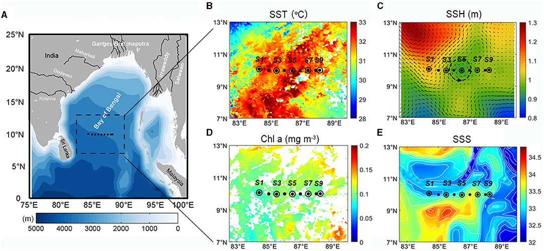
Figure 1. (A) Bathymetry, (B) MODIS sea surface temperature (SST, °C), (C) AVISO sea surface height (SSH, m) with geostrophic currents (m s−1), (D) MODIS sea surface Chl a (mg m−3), and (E) CMEMS modeling sea surface salinity (SSS) in the study region. The dots in black indicate CTD sampling stations, while black circles are additional chemical and biological samplings.
CTD Sampling
Hydrographic data, including temperature and salinity, along the transect were collected through a Sea-Bird 911 plus conductivity-temperature-depth profiler (CTD, Belleview, WA, USA). Fluorescence and dissolved oxygen were also measured along with the CTD. These data were binned every 1 m depth.
Nutrients and Chl a Sampling and Analyses
Water samples from seven depths [5, 25, 50 m, deep Chl a maximum (DCM) depth, 100, 150, and 200 m] at stations S1, S3, S5, S7, and S9 were collected using an 8-L Niskin bottle (Hydro-Bio, Altenholz, Germany) mounted on the CTD. The in situ DCM depth was determined using the fluorescence profiles from CTD sensor. The seawater (100 ml) from each of the Niskin bottles was immediately stored in pickled polyethylene bottles and frozen at −20°C in the dark for further nutrient analyses in the laboratory. Dissolved inorganic nitrate (NO3), silicate (SiO3) and soluble reactive phosphorus (SRP) were then measured with an autoanalyzer (QuickChem 8500, Lachat Instruments, Milwaukee, WI, USA) (Kirkwood et al., 1996).
For the size-fractionated Chl a from micro- (>20 μm), nano- (3–20 μm), and pico-phytoplankton (0.7–3 μm), 500 or 1,000 ml of sampled seawater were sequentially filtered through polycarbonate membranes with pore sizes of 20 and 3 μm (Osmonics Inc., Macungie, PA, USA) and glass-fiber filters with a pore size of 0.7 μm (Whatman plc, Little Chalfont, Buckinghamshire, UK). The filters were wrapped in aluminum foil and stored at −20°C in the dark until they were analyzed in the laboratory. The filtered samples were then extracted with 90% acetone, sonicated for 15 min, and stored overnight at −20°C in the dark. The Chl a was then measured using a Turner Designs Model 10 Fluorometer (San Jose, CA, USA) (Parsons et al., 1984). The total Chl a concentration was calculated as the sum of these three size-fractionated values.
Zooplankton Sampling by Vertical Trawl
A plankton net with a mouth diameter of 80 cm and a mesh size of 300 μm was towed vertically from a depth of 200 m to the surface at a speed of ~1 m s−1 to collect zooplankton (Li et al., 2017). A flowmeter (Hydro-Bios, Altenholz, Germany) was mounted at the net mouth to estimate the volume of filtered water. The zooplankton samples were then preserved in a 5% formalin-seawater solution for laboratory analysis. All specimens were identified and counted based on the available taxonomic information from Li et al. (2017).
Zooplankton and Detritus Sampling and Determination by VPR
To examine the vertical distribution of zooplankton, a VPR (Seascan, Inc.) was also used to collect in situ images (Davis et al., 1996; Ashjian et al., 2001). The VPR was lowered vertically from the surface to a depth of ~800 m at a speed of ~1 m s−1. A camera with a larger field of view of ~46.5 × 34.5 mm (actual ~300 ml sampling volume) was chosen because this field size was the most productive based on the test sampling. The image data (including time and depth information) were processed and analyzed using the Visual Plankton software package. Automatic recognition and classification were performed based on our zooplankton image database, followed by manual calibration. The number of zooplankton was averaged for every 1 m depth. In this study, the upper 200 m of the imagery were used for the zooplankton analyses to compare with the net-sampling results.
The images of detritus collected by the VPR were processed in the same way as the zooplankton images. Based on the size (in pixels) of each individual particle in pixels and through image calibration, the actual sizes of the particles were obtained in mm. The equivalent spherical diameter (ESD) and equivalent spherical volume (ESV) were also obtained from the area of each individual particle. The sinking rate was then calculated using the formula m d−1 = 50ESD0.26 (Alldredge and Gotschalk, 1988), and the carbon content of each individual particle was estimated using the formula μg C = 0.99ESV0.52 (Alldredge, 1998). Furthermore, the concentrations of organic carbon (μg L−1) were obtained by coupling the abundances of the organic detrital particles and the carbon content of each individual particle, and the vertical organic carbon export flux (μg m−2 L−1) was calculated from the concentrations and organic carbon sinking rate. The concentration (μg L−1) and the vertical export flux (μg m−2 L−1) of organic carbon were then derived from the detrital abundance, the carbon content of individual particle, and their sinking rates.
Barrier Layer and Stability Calculation
Barrier layer thickness is equal to the difference between the isothermal layer depth (ILD) and mixed layer depth (MLD). The calculation of the MLD in this study was based on the UNESCO equation of state:
where Δσ represents the difference in density from the sea surface to the bottom of the mixed layer; the first term of the right hand of the equation represents the density of the seawater when the temperature changes ΔT (1.2°C) relative to the surface while the salinity remains constant; the second term represents the sea surface density. The T0, S0, and P0 are sea surface temperature, salinity, and pressure, respectively. The depth of the mixed layer is the depth that corresponds to the surface density minus Δσ. The ILD is the depth obtained by subtracting the same ΔT from the sea surface temperature.
The state stability parameter was calculated based on the formula from Pond and Pickard (1983):
where E is the state stability parameter (m−1), ρ is the density of seawater (kg m−3), and z is the depth (m).
One-Dimensional Nutrient-Phytoplankton-Detritus Model
To study the mechanism and processes of how barrier layers affect the biological production and carbon export in the upper ocean, an idealized one-dimensional vertical nutrient-phytoplankton-detritus (NPD) ecosystem model, based on Beckmann and Hense (2007), was used:
where N is the limiting nutrient, P is phytoplankton, and D is detritus (all in units of mmol N m−3). In simplified marine ecosystem models, the biomass of zooplankton is usually regarded as a proportion of phytoplankton biomass, so zooplankton is not explicitly included in this simple model. σL and σN are the growth limitations for nutrients and light, respectively, with functions:
The Photosynthetically Active Radiation (PAR) decreases with depth:
According to the sensitivity experiments of Beckmann and Hense (2007), the proper values of the parameters in the above equations and functions are chosen to form a DCM layer in the upper ocean. The definition and values of the parameters used in this model are listed in Table 1.
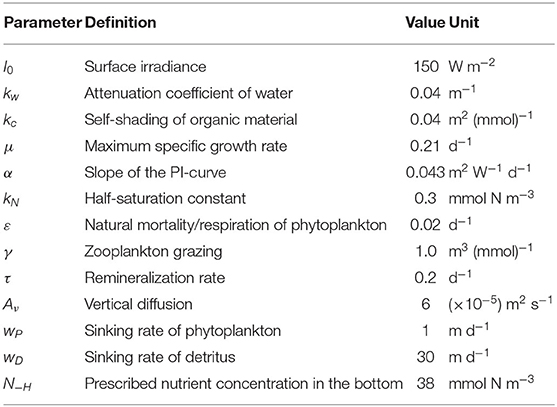
Table 1. Definition and values of parameters used in the model.
The fluxes at the surface boundary (z = 0) for all variables are zero. At the bottom boundary (z = −H, where H = 1,000 m), the phytoplankton flux is zero, and nutrient concentration is prescribed, and detritus is free to sink out of the domain. The vertical resolution in the model is 2 m. The initial concentrations of nutrients, phytoplankton, and detritus were set to be uniformly 0.1 mmol N m−3. The model was then integrated into a steady state (differences between successive time steps of vertically integrated phytoplankton content reach within 10−8%). This steady-state solution was seen as a representation of the basic ecosystem structure in the upper ocean under a weak mixing and oligotrophic condition that is not affected by the BL (“unaffected scenario”).
To evaluate the effects of the barrier layer in the upper ocean, we set a special layer, in which the vertical diffusion coefficient Aν was much smaller than other depths. This special layer was set to be located at depths between 20 and 40 m and the vertical diffusion Aν in this layer was 2 × 10⁻⁵ m2 s−1, which was one-third of that at other depths. After initializing with the steady-state solution of the unaffected scenario, the model was then restarted to achieve a new steady solution, which was referred to as “the BL-affected scenario.” Moreover, a series of sensitivity tests on the thickness of this layer and the value of its vertical diffusion were conducted to assess the impact of the BL thickness on ecosystem structures. The thickness varied from 10 to 30 m with a fixed Aν (2 × 10⁻⁵ m2 s−1) and a varied Aν [1, 2, 4 (× 10−5 m2 s−1)], with 20 m in thickness being set in each sensitivity test.
Results
Physical Setting
The satellite data showed that the SST was generally high in the southern region of the BoB (south of 15°N) (Figure 1). The SSH and sea surface geostrophic current field demonstrated that a cyclone eddy passed through the survey transect. During the investigation period, the satellite-obtained sea surface Chl a concentration was low (<0.2 mg m−3) in the southern BoB. The SSS showed strong spatial gradient with high values (>34) in the southwest, northwest, and lower values (<32) in the east. The survey transect was located at the intersection of the salty and freshwater bodies, while the sea surfaces at some stations were covered by freshwater (salinity <33).
The in situ data collected along the transect showed that the stations capped by freshwater had lower surface Chl a concentrations (Figure 2). The salinity was quite low within the upper 20 m (lowest was 32.2) except for stations S6 and S7 (~34). The vertical salinity gradient in these stations reached their maximums at 10–20 m and formed a surface halocline. The fluorescence had a very similar pattern to that of the salinity in the surface layer, with relatively higher values at stations S6 and S7. The surface temperature along the survey transect was high (>30°C), and values that exceeded 31°C were observed at some stations. The dissolved oxygen (DO) concentrations in the surface layer were also high (5–6 mg L−1) but exhibited no horizontal differences.
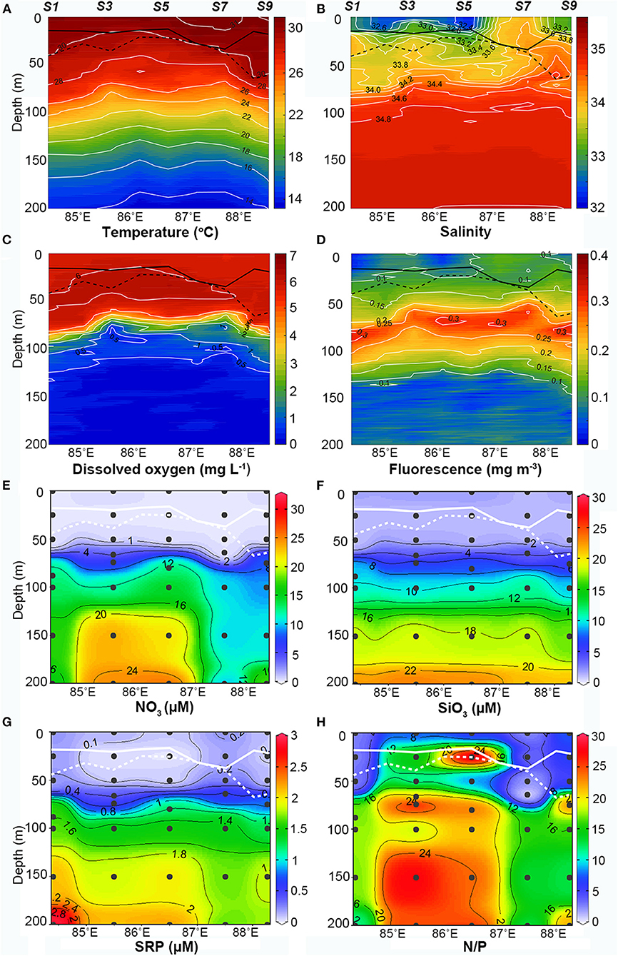
Figure 2. Vertical profiles of in situ (A) temperature (°C), (B) salinity, (C) dissolved oxygen (mg L−1), (D) fluorescence, (E) nitrate (μM), (F) silicate (μM), (G) dissolved reactive phosphorous (μM), and (H) ratio of nitrate to dissolved reactive phosphorus (N/P) to P along the section in the upper 200 m. The solid and dashed lines plotted in each panel represent mixed layer depth and isothermal depth, respectively.
The temperature, salinity, and DO isoclines upheaved distinctly around stations S3 and S4 but failed to outcrop. The 30°C isotherm shallowed from ~50 m at station S1 to ~20 m at stations S3 and S4. Isohalines (33), isolines of DO (6 mg L−1), and fluorescence isolines (0.1 mg m−3) also showed obvious shoaling in this region. This might be due to the passing of the cyclonic eddy observed by the satellite (Figure 1C). Although the near surface isohalines shallowed, they failed to break through the surface low-salinity water mass and were still suppressed below the surface. At depths of 80–100 m, the temperature gradient and those of salinity and DO varied significantly, subsequently forming a deep thermocline, halocline, and DO-cline. At the same depth, fluorescence reached its maximum and formed the DCM layer. The DCM layers uplifted at station S3 and S7 but were thinner at station S3 compared to station S7. Below the DCM layer, the temperature gradually decreased from 22 to 14°C, while the salinity remained between 34.8 and 35 with no marked horizontal variations. Meanwhile, the DO decreased to an extremely low level (<0.1 mg L−1) and the fluorescence also decreased rapidly.
Barrier Layer
Barrier layers were formed beneath the MLD at the freshwater-capped sampling stations and enhanced the stability of the upper water column. According to equation (1), the MLDs at the surveyed stations were relatively shallow (<36 m) during the survey period (Figure 2, solid black line) and shoaled to <20 m at freshwater-capped stations. The ILD (black dotted line) had a very different trend. It was deeper than MLD at most stations, except at stations S6 and S7, where the surface salinities were much higher. The BL thickness, derived from the difference of MLD and ILD, ranged from 0 to 48 m along the survey transect, with an average of 18 m. While the average BL thickness at the freshwater-capped stations was ~23 m, the same thickness at stations without freshwater cap was negligible at only ~1 m. Based on the calculated BL thickness, S1 (25.6 m), S2 (13.1 m), S3 (18.3 m), S4 (7.0 m), S5 (8.9 m), S8 (47.8 m), and S9 (41.7 m) were referred to as the BL-affected stations, while S6 (0 m) and S7 (3 m) were referred to as the unaffected stations (Figure 2). Calculated from equation (2), the stability parameter of the surface water at the BL-affected station S3 was 1.5 × 10⁻⁴, which was much larger than that at the unaffected station S7 (<0.4 × 10⁻⁴). It even exceeded the deep stability parameter (1.18 × 10⁻⁴), which was caused by the thermocline at a depth of ~70 m at station S3 (Figure 3, dashed line).
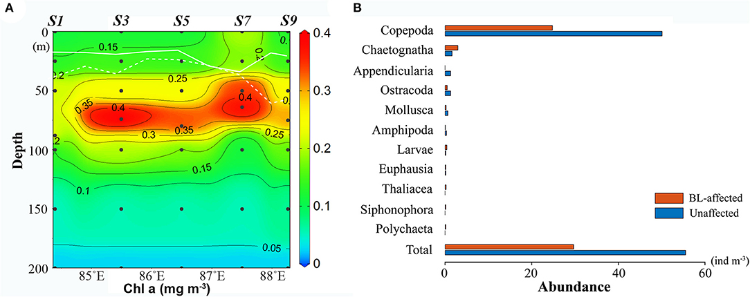
Figure 3. Comparison of the vertical profiles of nitrate (cyan), silicate (yellow), soluble reactive phosphorous (SRP) (red), Chl a (lime), salinity (black, solid), and stability parameter (black, dashed) at the BL-affected station S3 (A) and unaffected station S7 (B), only the upper 100 m are shown. The depth and thickness of the BL at station S3 are indicated.
Vertical Profiles of Nutrients
The vertical distributions of the nutrients had prominent disparities between the BL-affected and -unaffected stations. The concentrations of NO3, SiO3, and SRP generally increased with depth. An intense nutricline appeared at depths of 50–60 m, above which the concentrations of all the nutrients became fairly low and almost depleted. However, the concentrations of SRP at stations S1 and especially S7 (>0.2 μM) were higher than those at the other stations (<0.1 μM), though the minimum value still occurred in the near-surface layer. Furthermore, NO3 was extremely depleted above the nutricline, and the minimum concentration below 0.2 μM occurred in the 25–50-m layer. However, the surface concentration of NO3 increased slightly at stations S3 and S9 (~0.5 μM). Above the nutricline, the concentrations of SiO3 (<2 μM) were also quite low but higher than NO3. Similar to NO3, the surface concentrations of SiO3 (~2 μM) at all stations except S7 appeared to be higher than in the 25 and 50 m layers (~1 μM). Below the nutricline, the concentrations of all three nutrients increased considerably, while there was a deep increase in NO3 and SRP at stations S1–S5. The ratio of NO3 to SRP (N/P) above the nutricline was generally low (<5), but it increased in the near-surface layers at stations S3 and S5. While the N/P ratio in the deep waters below the nutricline increased and exceeded the Redfield ratio (~16), especially at stations S3 and S5, station S7 did not show such an increase.
Vertical Distribution of Chl a
The Chl a concentrations were lower and the DCM layers were deeper and thinner at the BL-affected stations. The total Chl a concentration was generally low in the upper 25-m layer (Figure 4A) and even lower (<0.15 mg m−3) in the BL-affected stations. The DCM layers in our study regions varied from 40 to 90 m. The DCM layers (> 0.3 mg m−3) at the BL-affected stations (70–90 m) were deeper than at the unaffected stations (40–80 m). Moreover, the DCM layers at the BL-affected stations (20 m) were remarkably thinner compared to that of the unaffected stations (40 m). The vertical distribution of sized-fractionated Chl a concentrations (not shown) were also consistent with that of the total Chl a. Among the size fractions, the pico-phytoplankton accounted for the majority of the total Chl a (>70%). The concentrations of micro- and nano-phytoplankton were both quite low (<0.1 mg m−3), while each accounted for only ~10% of the total phytoplankton concentration. The average vertically integrated Chl a concentrations in the BL-affected stations (0.15 mg m−3) were ~18% lower than those at the unaffected stations (0.18 mg m−3) in the upper 200 m.
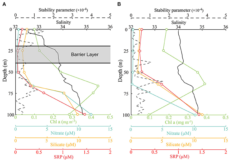
Figure 4. (A) Vertical distribution of total Chlorophyll a (Chl a) (mg m−3) along the transect (the solid and dashed lines in white represent the mixed layer depth and isothermal depth, respectively); (B) abundances of zooplankton taxonomic groups at the barrier layer (BL)-affected station S3 and the unaffected station S7.
Abundance and Vertical Distribution of Zooplankton
Zooplankton abundances were remarkably lower while zooplankton composition was altered at BL-affected stations (Figure 4B). Net-sampled zooplankton in the upper 200 m consisted of Copepods, Chaetognaths, Appendicularia, Ostracoda, Mollusca, Amphipoda, Polychaeta, Euphausia, Thaliacea, Siphonophora, and Larvae. Copepods were the most dominant group (83–90%), followed by Chaetognatha (3–10%), Ostracoda (1–3%), and Appendicularia (0–3%). The copepods abundance at the BL-affected stations (24.8 ind. m−3) was less than half of the abundance at the unaffected stations (50.08 ind. m−3). The abundances of Appendicularia, Ostracoda, and Mollusca and their contributions to the total zooplankton abundance were also lower at BL-affected stations. However, the abundance of Chaetognaths was higher at the BL-affected stations while their proportion to the total abundance reached 10%, which was much higher than that at the unaffected stations (3%). The abundances of the other groups were rather low during the sampling period. The total zooplankton abundances at the BL-affected and -unaffected stations were 29.68 and 55.52 ind. m−3, respectively.
To rule out of the diel vertical migration effect of zooplankton, station S3 and S7 (both sampled during daytime) were selected as the representative BL-affected and -unaffected stations, respectively, for the VPR analyses. Copepods and detritus were the most abundant groups captured by VPR imaging. Copepod abundances observed using the VPR were very low at BL-affected station S3 and were mainly distributed above the DCM layer. The average abundance of copepods in the upper 200 m was 5.17 ind. m−3 at station S3 and 24.15 ind. m−3 at station S7, both of which were lower than the net-sampled abundances. This may be partly due to the selection of a larger viewing field; such that smaller copepods could not be clearly identified. However, consistent with the results of the net-sampled zooplankton, the VPR observations also showed that the copepod abundance at the BL-affected station was much less than that of the unaffected station. Copepods were mainly distributed above the depths of the DCM layer at both stations (Figure 5). Additionally, maximum copepods abundance occurred in the surface layer at station S7, but no maximum was apparent at station S3.
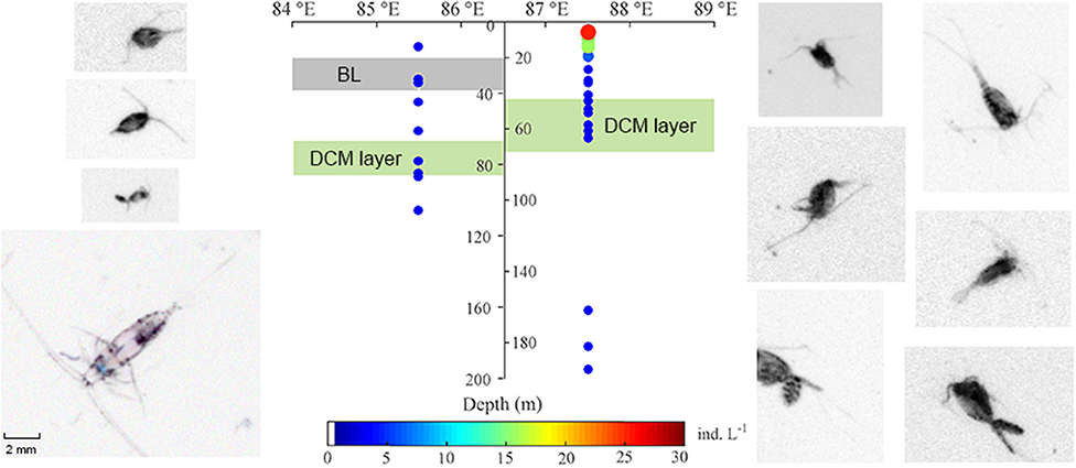
Figure 5. Comparison of vertical distribution and abundance of copepods from the video plankton recorder (VPR) in the upper 200 m at the BL-affected and -unaffected stations. The shaded gray indicates the depth and thickness of the BL, while the shaded lime indicates the depth and thickness of the deep Chl a maximum (DCM) layers. Copepod photos were taken from the sampling stations and their colors have been inverted to capture more details.
Vertical Distribution of Detritus and Particulate Organic Carbon Fluxes From Euphotic Zone
A lower abundance of detritus was observed at the BL-affected station compared with the unaffected station. The average size of individual detrital particles (ESD) captured in the upper 800 m was ~2.28 mm with 2.39 ± 0.77 mm at station S3 and 2.24 ± 0.52 mm at station S7 (Table 2). The average carbon content per individual detrital particle calculated from the detrital particles size was 3.01 ± 1.36 μg C ind.−1 at station S3 and 2.58 ± 0.88 μg C ind.−1 at station S7. Figure 6 depicts the vertical distribution of detrital particles and carbon concentrations at both stations. Although no significant differences in particle sizes were found between these two stations (p > 0.05; t-test), much higher detrital particle abundances (two-fold) in the carbon concentrations were observed at station S7, which was consistent with the higher abundance of net-captured zooplankton. Moreover, the detrital particles only occurred below 100 (S3) and 60 m (S7), both of which were below the depth of the DCM layers, and scarce detritus particles were observed below 500 m at both stations (Supplementary Figure 1).
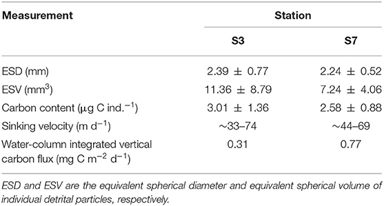
Table 2. Measurements of detritus and associated carbon flux at the BL-affected station and the unaffected station in the upper 800 m.
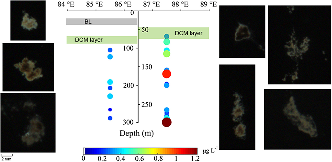
Figure 6. Vertical distribution of detritus abundance in carbon concentration in the upper 300 m at the BL-affected station and the unaffected station. The BL and DCM layers were shown by shaded gray and lime, respectively, as the same as those in Figure 5. Photos of detrital particles were extracted from the sampling stations.
Higher carbon export fluxes were estimated at the unaffected station compared with the BL-affected station. The sinking rates of the detrital particles ranged from 33 to 74 m d−1 at station S3 and from 44 to 69 m d−1 at station S7. Considering the much higher detrital abundances at station S7, the average vertical carbon export flux from the upper ocean (800 m) to the deep ocean was remarkably lower at station S3 (0.31 mg C m−2 d−1) compared with that at station S7 (0.77 mg C m−2 d−1).
Model Results
The steady-state solution of the unaffected scenario (Figure 7A, solid line) represented the vertical distribution of nutrient, phytoplankton, and detritus well in a weak mixing oligotrophic ocean and resembled our observations at the unaffected stations. With an extremely low concentration at the surface, the nutrient gradually increased with depth. The phytoplankton concentration also increased with depth as the nutrient limitation relaxed and then reached its maximum in the subsurface, forming a DCM layer. Below this maximum layer, the concentration decreased rapidly when the light became the dominant limiting factor. The vertical distribution of detritus followed the phytoplankton, but its maximum was located about 30 m deeper than the DCM layer. Below the detritus maximum, the amount of detritus decreased slowly with depth, forming a long tail.
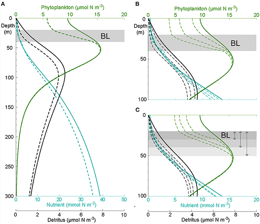
Figure 7. (A) Modeled vertical distribution of nutrients (blue), phytoplankton (green), and detritus (black) not affected (solid) and affected by the BL (dashed) in the upper 300 m. Sensitivity of the model solutions to the (B) vertical diffusion [1, 2, 4 (× 10−5 m2 s−1)] and (C) thickness (10, 20, and 30 m) of the BL, only the upper 100 m are shown.
The existence of a BL altered the vertical distribution of phytoplankton in the upper ocean and nutrient and detritus in the whole domain (Figure 7A, dashed line). After adding a BL at depths of 20–40 m, the model gained a new steady solution quickly. The new steady state showed that the nutrient above the BL was depleted to an even lower level but slightly enhanced beneath the layer. This was due to the inhibition of upward nutrient transport by the BL, leading to the accumulation of nutrients underneath. Furthermore, the phytoplankton concentration significantly decreased in the surface because of the depleted nutrients, as this decrease then went down to the DCM layer, subsequently leading to a thinner and slightly smaller DCM layer. This, in turn, resulted in an ~22% decrease of the phytoplankton biomass above the DCM layer. Not surprisingly, the decrease of phytoplankton above the DCM layer led to a notable decrease (~20%) of detritus in the whole model domain. The decrease of the nutrient below the DCM layer was due to reduced remineralization, which relied on the concentration of detritus.
The sensitivity tests showed that both the vertical diffusion in the BL and the thickness of the BL affected the ecosystem productivity in the upper ocean: a smaller vertical diffusion (stronger stability) in the BL (Figure 7B) or a thicker BL (Figure 7C) led to a lower concentration of nutrients above the BL and below the DCM layer, a reduced phytoplankton concentration above the DCM layer and a thinner DCM layer, and a diminished detritus concentration in the whole column. Furthermore, the magnitude of the DCM layer was reduced when the vertical diffusion became smaller.
Discussion
By comparing the environmental and biological parameters at the BL-affected and -unaffected stations, we found that the BL-affected regions experienced lower nutrient concentrations in the upper layers, lower phytoplankton biomasses in the surface layer, and thinner DCM layers. The zooplankton and detrital abundances were also lower in the BL-affected regions. Subsequently, a one-dimensional vertical NPD model was used to validate the observed results. The results indicated that the BL reduced the biological production by weakening vertical mixing and associated nutrient supplies. The BL, thus, has an inhibitory effect on carbon export to the deep ocean in the BoB. This study could be a strong piece of evidence that explains the impact of a BL on biological production and carbon export in this region. The results also suggest that more attention should be paid to the effects of BLs on the biological production and biogeochemical cycle in tropical and polar oceans, as freshwater input and surface stratification are predicted to increase along with the global warming (Wentz et al., 2007; Trenberth, 2011; Yamaguchi and Suga, 2019; Li et al., 2020).
Barrier layers strongly enhance stability and inhibit vertical mixing in the upper ocean. George et al. (2019) had previously measured the turbulent mixing to be much smaller in the BL compared with that in the mixed layer. In contrast, the current study also showed that the existence of BL strengthened the stability of the upper water column (Figure 3). The depletion of dissolved inorganic nutrients in surface waters and the rapid decrease of DO in the upper layer at 80–100 m suggested the strong surface stability and inhibited vertical mixing in the upper ocean within the study region. If no intense external perturbations such as tropical cyclones or eddies were present (Prasanna Kumar et al., 2007; Vissa et al., 2013), the BL would not be easily destroyed, even during the winter when the strong northeast monsoon dominates and the surface temperatures drop (Thadathil et al., 2002; Girishkumar et al., 2013). In this study, a cyclonic eddy did pass through the study region, leading to shallower ILDs and thinner BLs at stations S3 and S4 (Figure 2). However, this eddy was pretty weak and did not break up the BL, while the strong near-surface halocline was maintained. Although the advection of freshwater may lead to high shear at the interfaces, the strong stratification can overcome the destabilizing influence of these shear regions (George et al., 2019).
The concentrations of SRP at unaffected stations, such as S7, were much higher than those at the BL-affected stations, suggesting that BLs prevent the vertical transport of nutrients. During the study period, dissolved inorganic nutrients above the nutricline had low concentrations. The replenishment of the surface nutrients in the open areas of the BoB was highly dependent on the vertical transport of deep, nutrient-rich water. Inhibited by the BL, vertical transport and mixing were weakened in the upper layers. This depletion of SRP in the upper 50 m and the suppression and deepening of the phosphate nutricline were observed at the BL-affected stations. Although the observation results were from limited stations, the one-dimensional NPD model in this study successfully simulated the lowered surface nutrient concentrations and downward movements of nutricline induced by the BL. Slightly higher residual concentrations of nitrate and silicate, but larger depletions of SRP in surface waters, at the BL-affected stations indicated that the low-salinity surface waters at these stations may have originated from river runoffs. This is because river runoffs contain relatively higher concentrations of nitrate and silicate (Liu et al., 2009; Sarma et al., 2010). Furthermore, dissolved inorganic phosphorus is often depleted first, while nitrate and silicate remained when the freshwater plume arrived in the study region. The occurrence of a Trichodesmium bloom during the survey could also support this argument, as the nitrogen fixer Trichodesmium can out-compete other phytoplankton for dissolved organic phosphorus without nitrogen and, therefore, has an advantage in waters with low dissolved inorganic phosphorus concentrations (Dyhrman et al., 2006; Orchard et al., 2010).
A barrier layer results in low epipelagic biological production by inhibiting vertical nutrient supplies. In weakly mixed open seas, a DCM layer usually occurs above the nutricline, and its depth, thickness, and intensity are controlled by water column stability (Beckmann and Hense, 2007; Gong et al., 2015; Thushara et al., 2019; Amol et al., 2020). It was observed that the DCM layers were thinner and deepened in the BL-affected regions, while the Chl a concentrations above the DCM layers were notably lower in these regions (Figure 4). In regions affected by the eddy (station S3), the DCM layer was lifted but the surface Chl a was still suppressed by the BL (Figures 2D, 4A). The model of this study successfully simulated the decreased surface Chl a and squeezed DCM layer, but not the significant deepening of the DCM layer. The observed deepening of the DCM layer, coupled with deepened thermocline and DO-cline in freshwater-covered regions (except for the cyclone-affected stations; Figure 2), might be due to the horizontal advection of freshwater that pushed the water column downward. The results from our model revealed that a single surface stratification (without freshwater covering the surface) can cause decreased surface phytoplankton biomasses and squeezed DCM layers. As a result of stratification, low secondary production, which is indicated by low zooplankton abundance, was also observed in the BL-affected regions. Both the net-sampling and VPR observations showed that the zooplankton abundances in the BL-affected regions were much lower than those of the unaffected regions. Sarma et al. (2016) also observed fewer mammals in regions covered by freshwater, indicating that the existence of a BL might influence fishery resources due to reduced primary (carbon fixation) and secondary productions in the upper ocean. Furthermore, the results of the net-captured zooplankton taxonomic compositions and abundances were consistent with previously reported results in the study region (Fernandes, 2008; Li et al., 2017). The study also indicated that the VPR observations had advantages for imaging the vertical trends of zooplankton, although the VPR-observed abundance values were smaller than those obtained using net-sampling.
Consistent with the decreased biological production, the detrital abundance as marine snow and the organic carbon export from the euphotic zone to the deep ocean were remarkably lower in the BL-affected regions. The estimated organic carbon sinking rates (0.31–0.77 mg C m−2 d−1) in the BoB during spring were lower than the findings reported by Anand et al. (2017). This might be due to the difficulty of capturing all detrital particles using real-time video observation techniques. However, optical instruments can deliver a much greater spatial and temporal coverage of particles in the ocean than traditional techniques (Briggs et al., 2020; Giering et al., 2020). The detritus with higher abundance below the DCM layer (both indicated by the VPR and the model), coupled with high zooplankton abundance, suggests the linkage between carbon flux and the productivity of the upper ocean (Ittekkot et al., 1991; Ashjian et al., 2001; Sarma et al., 2014). In the BL-affected regions, the decrease in biological production reduced the amount of detritus produced by dead plankton and feces. Moreover, the remineralization of sinking coarser detritus in highly stratified waters occurring below the thermocline led to the formation of the oxygen minimum zones (OMZs) and the dominance of heterotrophy (Sarma, 2002; Anand et al., 2017). The occurrence of the Trichodesmium bloom during the survey and the lowered oxygen concentration beneath the thermocline at station S3 (Figure 2C) also indicated a more severe dominance of heterotrophy in the BL-affected regions. Therefore, the organic carbon in the BL-affected regions might undergo more intermediate steps in the micro-food web before passing to the higher trophic level, resulting in a prolonged organic carbon residence time and a reduced vertical organic carbon export (Jyothibabu et al., 2008; Anand et al., 2017; Middelbo et al., 2018; Fragoso et al., 2019).
Conclusions
This study systematically investigated the effects of the barrier layer on biological production and organic carbon export through in situ observations and a numerical model. The existence of a BL restricted vertical mixing and nutrient transport, causing the inorganic nutrients in the upper layers to be completely consumed or be present at extremely low concentrations. The reduced surface phytoplankton concentration and squeezed DCM layer produced a decrease in carbon fixation in the upper ocean, causing a reduction in zooplankton abundance. The use of a VPR also gave a better understanding of the vertical distribution of zooplankton and detrital particles that are affected by a BL. The decrease in the vertical carbon export flux rates caused by detrital deposition indicates that BLs exert a non-negligible effect on the ocean biogeochemical progresses and carbon cycle. More comprehensive studies on the effects of BLs on biological production processes and ocean biogeochemical cycles are suggested in regions affected by high precipitations and freshwater flux. As high precipitation and freshwater inputs are predicted to increase in tropical and polar oceans with global warming, the greater impacts of BLs on the global epipelagic ecosystem, marine fishery resources, biogeochemical progresses, and carbon cycles might be expected.
Data Availability Statement
The raw data supporting the conclusions of this article will be made available by the authors, without undue reservation.
Author Contributions
HZ conceived of the presented idea. HZ and LZ collected the in situ samplings. HZ, LZ, ZK, and KL analyzed the samplings. HZ processed the data, performed the analysis, drafted the manuscript, and designed the figures. LZ and YT revised the manuscript. All authors provided critical feedback, helped to shape the research, contributed to the article, and approved the submitted version.
Funding
This work was jointly funded by the National Natural Science Foundation of China (Nos. 31971432 and 41506161), Southern Marine Science and Engineering Guangdong Laboratory, Guangzhou (Nos. GML2019ZD0405), Guangdong marine economy promotion projects Fund (No. GDOE[2019]A32), and Science and Technology Planning Project of Guangdong Province, China (No. 2017B0303014052).
Conflict of Interest
The authors declare that the research was conducted in the absence of any commercial or financial relationships that could be construed as a potential conflict of interest.
Publisher's Note
All claims expressed in this article are solely those of the authors and do not necessarily represent those of their affiliated organizations, or those of the publisher, the editors and the reviewers. Any product that may be evaluated in this article, or claim that may be made by its manufacturer, is not guaranteed or endorsed by the publisher.
Acknowledgments
We would like to thank the crew of the Shiyan 3 for their assistance with the sampling by CTD. MODIS-Aqua Level-3 sea surface temperature and Chl a are from http://oceancolor.gsfc.nasa.gov/. SSH and geostrophic current data are from http://www.aviso.altimetry.fr. Numerical-model salinity is from http://marine.copernicus.eu.
Supplementary Material
The Supplementary Material for this article can be found online at: https://www.frontiersin.org/articles/10.3389/fmars.2021.710051/full#supplementary-material
References
Alldredge, A. (1998). The carbon, nitrogen and mass content of marine snow as a function of aggregate size. Deep Sea Res. Part I Oceanogr. Res. Pap. 45, 529–541. doi: 10.1016/S0967-0637(97)00048-4
Alldredge, A. L., and Gotschalk, C. (1988). In situ settling behavior of marine snow. Limnol. Oceanogr. 33, 339–351. doi: 10.4319/lo.1988.33.3.0339
Amol, P., Vinayachandran, P. N., Shankar, D., Thushara, V., Vijith, V., Chatterjee, A., et al. (2020). Effect of freshwater advection and winds on the vertical structure of chlorophyll in the northern Bay of Bengal. Deep Sea Res. Part II: Top. Stud. Oceanogr. 179:104622. doi: 10.1016/j.dsr2.2019.07.010
Anand, S. S., Rengarajan, R., Sarma, V. V. S. S., Sudheer, A. K., Bhushan, R., and Singh, S. K. (2017). Spatial variability of upper ocean POC export in the Bay of Bengal and the Indian Ocean determined using particle-reactive 234Th. J. Geophys. Res. Oceans 122, 3753–3770. doi: 10.1002/2016JC012639
Ashjian, C. J., Davis, C. S., Gallager, S. M., and Alatalo, P. (2001). Distribution of plankton, particles, and hydrographic features across Georges Bank described using the Video Plankton Recorder. Deep Sea Res. Part II: Top. Stud. Oceanogr. 48, 245–282. doi: 10.1016/S0967-0645(00)00121-1
Balaguru, K., Chang, P., Saravanan, R., and Jang, C. J. (2012). The Barrier Layer of the Atlantic warm pool: formation mechanism and influence on the mean climate. Tellus Ser. A-Dyn. Meteorol. Oceanol. 64:18162. doi: 10.3402/tellusa.v64i0.18162
Balaguru, K., Foltz, G. R., Leung, L. R., and Emanuel, K. A. (2016). Global warming-induced upper-ocean freshening and the intensification of super typhoons. Nat. Commun. 7:13670. doi: 10.1038/ncomms13670
Beckmann, A., and Hense, I. (2007). Beneath the surface: characteristics of oceanic ecosystems under weak mixing conditions—a theoretical investigation. Prog. Oceanogr. 75, 771–796. doi: 10.1016/j.pocean.2007.09.002
Behara, A., and Vinayachandran, P. N. (2016). An OGCM study of the impact of rain and river water forcing on the Bay of Bengal. J. Geophys. Res. Oceans 121, 2425–2446. doi: 10.1002/2015JC011325
Bindoff, N. L., Cheung, W. W. L., Kairo, J. G., Arístegui, J., Guinder, V. A., Hallberg, R., et al. (2019). Changing ocean, marine ecosystems, and dependent communities, in IPCC Special Report on the Ocean and Cryosphere in a Changing Climate, eds. H.-O. Pörtner, D. C. Roberts, V. Masson-Delmotte, P. Zhai, M. Tignor, E. Poloczanska, et al., 447–587
Briggs, N., Dall'Olmo, G., and Claustre, H. (2020). Major role of particle fragmentation in regulating biological sequestration of CO2 by the oceans. Science 367, 791–793. doi: 10.1126/science.aay1790
Cabrera, O., Villanoy, C., David, L., and Gordon, A. (2011). Barrier Layer Control of Entrainment and Upwelling in the Bohol Sea, Philippines. Oceanography 24, 130–141. doi: 10.5670/oceanog.2011.10
Davis, C. S., Gallager, S. M., Marra, M., and Kenneth Stewart, W. (1996). Rapid visualization of plankton abundance and taxonomic composition using the Video Plankton Recorder. Deep-Sea Res. Part II: Top. Stud. Oceanogr. 43, 1947–1970. doi: 10.1016/S0967-0645(96)00051-3
Dekshenieks, M. M., Donaghay, P. L., Sullivan, J. M., Rines, J. E. B., Osborn, T. R., and Twardowski, M. S. (2001). Temporal and spatial occurrence of thin phytoplankton layers in relation to physical processes. Mar. Ecol. Prog. Ser. 223, 61–71. doi: 10.3354/meps223061
Dyhrman, S. T., Chappell, P. D., Haley, S. T., Moffett, J. W., Orchard, E. D., Waterbury, J. B., et al. (2006). Phosphonate utilization by the globally important marine diazotroph Trichodesmium. Nature 439, 68–71. doi: 10.1038/nature04203
Fernandes, V. (2008). The effect of semi-permanent eddies on the distribution of mesozooplankton in the central Bay of Bengal. J. Mar. Res. 66, 465–488. doi: 10.1357/002224008787157430
Fragoso, G. M., Davies, E. J., Ellingsen, I., Chauton, M. S., Fossum, T., Ludvigsen, M., et al. (2019). Physical controls on phytoplankton size structure, photophysiology and suspended particles in a Norwegian biological hotspot. Prog. Oceanogr. 175, 284–299. doi: 10.1016/j.pocean.2019.05.001
Fu, W., Randerson, J. T., and Moore, J. K. (2016). Climate change impacts on net primary production (NPP) and export production (EP) regulated by increasing stratification and phytoplankton community structure in the CMIP5 models. Biogeosciences 13, 5151–5170. doi: 10.5194/bg-13-5151-2016
Gauns, M., Madhupratap, M., Ramaiah, N., Jyothibabu, R., Fernandes, V., Paul, J. T., et al. (2005). Comparative accounts of biological productivity characteristics and estimates of carbon fluxes in the Arabian Sea and the Bay of Bengal. Deep Sea Res. Part II: Top. Stud. Oceanogr. 52, 2003–2017. doi: 10.1016/j.dsr2.2005.05.009
George, J. V., Vinayachandran, P. N., Vijith, V., Thushara, V., Nayak, A. A., Pargaonkar, S. M., et al. (2019). Mechanisms of barrier layer formation and erosion from in situ observations in the Bay of Bengal. J. Phys. Oceanogr. 49, 1183–1200. doi: 10.1175/JPO-D-18-0204.1
Giering, S. L. C., Cavan, E. L., Basedow, S. L., Briggs, N., Burd, A. B., Darroch, L. J., et al. (2020). Sinking organic particles in the ocean—flux estimates from in situ optical devices. Front. Mar. Sci. 6:834. doi: 10.3389/fmars.2019.00834
Girishkumar, M. S., Ravichandran, M., and McPhaden, M. J. (2013). Temperature inversions and their influence on the mixed layer heat budget during the winters of 2006–2007 and 2007–2008 in the Bay of Bengal. J. Geophys. Res.-Oceans 118, 2426–2437. doi: 10.1002/jgrc.20192
Godfrey, J. S., Houze, R. A., Johnson, R. H., Lukas, R., Redelsperger, J. L., Sumi, A., et al. (1998). Coupled ocean-atmosphere response experiment (COARE): an interim report. J. Geophys. Res.-Oceans 103, 14395–14450. doi: 10.1029/97JC03120
Godfrey, J. S., and Lindstrom, E. J. (1989). The heat budget of the equatorial western Pacific surface mixed layer. J. Geophys. Res. Oceans 94, 8007–8017. doi: 10.1029/JC094iC06p08007
Gong, X., Shi, J., Gao, H. W., and Yao, X. H. (2015). Steady-state solutions for subsurface chlorophyll maximum in stratified water columns with a bell-shaped vertical profile of chlorophyll. Biogeosciences 12, 905–919. doi: 10.5194/bg-12-905-2015
Ittekkot, V., Nair, R. R., Honjo, S., Ramaswamy, V., Bartsch, M., Manganini, S., et al. (1991). Enhanced particle fluxes in Bay of Bengal induced by injection of fresh water. Nature 351, 385–387. doi: 10.1038/351385a0
Jyothibabu, R., Madhu, N. V., Maheswaran, P. A., Jayalakshmy, K. V., Nair, K. K. C., and Achuthankutty, C. T. (2008). Seasonal variation of microzooplankton (20–200μm) and its possible implications on the vertical carbon flux in the western Bay of Bengal. Cont. Shelf Res. 28, 737–755. doi: 10.1016/j.csr.2007.12.011
Kara, A. B., Rochford, P. A., and Hurlburt, H. E. (2000). An optimal definition for ocean mixed layer depth. J. Geophys. Res. Oceans 105, 16803–16821. doi: 10.1029/2000JC900072
Kirkwood, D. S., Aminot, A., and Carlberg, S. R. (1996). The 1994 QUASIMEME Laboratory Performance Study: Nutrients in seawater and standard solutions. Mar. Pollut. Bull. 32, 640–645. doi: 10.1016/0025-326X(96)00076-8
Kumar, S. P., Muraleedharan, P. M., Prasad, T. G., Gauns, M., Ramaiah, N., Souza, S. N., et al. (2002). Why is the Bay of Bengal less productive during summer monsoon compared to the Arabian Sea? Geophys. Res. Lett. 29, 88–1–88-4. doi: 10.1029/2002GL016013
Li, G., Cheng, L., Zhu, J., Trenberth, K. E., Mann, M. E., and Abraham, J. P. (2020). Increasing ocean stratification over the past half-century. Nat. Clim. Chang. 10, 1116–1123. doi: 10.1038/s41558-020-00918-2
Li, K., Yin, J., Huang, L., Tan, Y., and Lin, Q. (2017). A comparison of the zooplankton community in the Bay of Bengal and South China Sea during April–May, 2010. J. Ocean Univ. China 16, 1206–1212. doi: 10.1007/s11802-017-3229-4
Liu, S. M., Hong, G.-H., Zhang, J., Ye, X. W., and Jiang, X. L. (2009). Nutrient budgets for large Chinese estuaries. Biogeosciences 6, 2245–2263. doi: 10.5194/bg-6-2245-2009
Lukas, R., and Lindstrom, E. (1991). The mixed layer of the western equatorial Pacific Ocean. J. Geophys. Res. Oceans 96, 3343–3357. doi: 10.1029/90JC01951
Mahadevan, A., Spiro Jaeger, G., Freilich, M., Omand, M., Shroyer, E., and Sengupta, D. (2016). Freshwater in the Bay of Bengal: its fate and role in air-sea heat exchange. Oceanography 29, 72–81. doi: 10.5670/oceanog.2016.40
Mann, K. H., and Lazier, J. R. N. (2013). Dynamics of Marine Ecosystems: Biological–Physical Interactions in the Oceans. Hoboken, NJ: John Wiley and Sons
Middelbo, A. B., Sejr, M. K., Arendt, K. E., and Moller, E. F. (2018). Impact of glacial meltwater on spatiotemporal distribution of copepods and their grazing impact in Young Sound NE, Greenland. Limnol. Oceanogr. 63, 322–336. doi: 10.1002/lno.10633
Miller, J. R. (1976). The salinity effect in a mixed layer ocean model. J. Phys. Oceanogr. 6, 29–35.
Montégut, C., de, B., Mignot, J., Lazar, A., and Cravatte, S. (2007). Control of salinity on the mixed layer depth in the world ocean: 1. General description. J. Geophys. Res. Oceans 112:C06011. doi: 10.1029/2006JC003953
Orchard, E. D., Ammerman, J. W., Lomas, M. W., and Dyhrman, S. T. (2010). Dissolved inorganic and organic phosphorus uptake in Trichodesmium and the microbial community: the importance of phosphorus ester in the Sargasso Sea. Limnol. Oceanogr. 55, 1390–1399. doi: 10.4319/lo.2010.55.3.1390
Parsons, T. R., Maita, Y., and Lalli, C. M. (1984). A Manual of Chemical and Biological Methods for Seawater Analysis. New York: Pergamon Press.
Pingree, R. D., Holligan, P. M., and Mardell, G. T. (1978). The effects of vertical stability on phytoplankton distributions in the summer on the northwest European Shelf. Deep Sea Res. 25, 1011–1028. doi: 10.1016/0146-6291(78)90584-2
Pond, S., and Pickard, G. L. (1983). Introductory Dynamical Oceanography. New York, NY: Pergamon Press.
Prasanna Kumar, S., Narvekar, J., Nuncio, M., Gauns, M., and Sardesai, S. (2009). What drives the biological productivity of the Northern Indian Ocean? Am. Geophys. Union Geophys. Monogr. Ser. 185, 33–56. doi: 10.1029/2008GM000757
Prasanna Kumar, S., Nuncio, M., Ramaiah, N., Sardesai, S., Narvekar, J., Fernandes, V., et al. (2007). Eddy-mediated biological productivity in the Bay of Bengal during fall and spring intermonsoons. Deep Sea Res. Part I Oceanogr. Res. Pap. 54, 1619–1640. doi: 10.1016/j.dsr.2007.06.002
Sarma, V. V. S. S. (2002). An evaluation of physical and biogeochemical processes regulating the oxygen minimum zone in the water column of the Bay of Bengal: physical and biogeochemical processes regulating the OMZ. Glob. Biogeochem. Cycles 16, 46–1–46-10. doi: 10.1029/2002GB001920
Sarma, V. V. S. S., Krishna, M. S., Prasad, V. R., Kumar, B. S. K., Naidu, S. A., Rao, G. D., et al. (2014). Distribution and sources of particulate organic matter in the Indian monsoonal estuaries during monsoon. J. Geophys. Res. Biogeosci. 119, 2095–2111. doi: 10.1002/2014JG002721
Sarma, V. V. S. S., Prasad, V. R., Kumar, B. S. K., Rajeev, K., Devi, B. M. M., Reddy, N. P. C., et al. (2010). Intra-annual variability in nutrients in the Godavari estuary, India. Cont. Shelf Res. 30, 2005–2014. doi: 10.1016/j.csr.2010.10.001
Sarma, V. V. S. S., Rao, G. D., Viswanadham, R., Sherin, C. K., Salisbury, J., Omand, M., et al. (2016). Effects of freshwater stratification on nutrients, dissolved oxygen, and phytoplankton in the Bay of Bengal. Oceanography 29, 222–231. doi: 10.5670/oceanog.2016.54
Thadathil, P., Gopalakrishna, V. V., Muraleedharan, P. M., Reddy, G. V., Araligidad, N., and Shenoy, S. (2002). Surface layer temperature inversion in the Bay of Bengal. Deep Sea Res. Part I: Oceanogr. Res. Pap. 49, 1801–1818. doi: 10.1016/S0967-0637(02)00044-4
Thushara, V., Vinayachandran, P. N., Matthews, A., Webber, B., and Queste, B. (2019). Vertical distribution of chlorophyll in dynamically distinct regions of the southern Bay of Bengal. Biogeosciences 16, 1447–1468. doi: 10.5194/bg-16-1447-2019
Trenberth, K. E. (2011). Changes in precipitation with climate change. Clim. Res. 47, 123–138. doi: 10.3354/cr00953
Vialard, J., and Delecluse, P. (1998). An OGCM study for the TOGA decade. Part II: Barrier-layer formation and variability. J. Phys. Oceanogr. 28, 1089–1106. doi: 10.1175/1520-0485(1998)028<1089:AOSFTT>2.0.CO;2
Vinayachandran, P. N. (2009). Impact of physical processes on chlorophyll distribution in the Bay of Bengal, in Geophysical Monograph Series, eds. J. D. Wiggert, R. R. Hood, S. W. A. Naqvi, K. H. Brink, and S. L. Smith (Washington, D. C.: American Geophysical Union), 71–86. doi: 10.1029/2008GM000705
Vinayachandran, P. N., Matthews, A. J., Kumar, K. V., Sanchez-Franks, A., Thushara, V., George, J., et al. (2018). BoBBLE: ocean–atmosphere interaction and its impact on the south asian monsoon. Bull. Am. Meteor. Soc. 99, 1569–1587. doi: 10.1175/BAMS-D-16-0230.1
Vissa, N. K., Satyanarayana, A. N. V., and Kumar, B. P. (2013). Response of upper ocean and impact of barrier layer on Sidr cyclone induced sea surface cooling. Ocean Sci. J. 48, 279–288. doi: 10.1007/s12601-013-0026-x
Wang, L., and Xu, F. (2018). Decadal variability and trends of oceanic barrier layers in tropical Pacific. Ocean Dyn. 68, 1155–1168. doi: 10.1007/s10236-018-1191-3
Webster, P., and Lukas, R. (1992). Toga Coare—the coupled Ocean atmosphere response experiment. Bull. Am. Meteorol. Soc. 73, 1377–1416. doi: 10.1175/1520-0477(1992)073<1377:TCTCOR>2.0.CO;2
Wentz, F. J., Ricciardulli, L., Hilburn, K., and Mears, C. (2007). How much more rain will global warming bring? Science 317, 233–235. doi: 10.1126/science.1140746
Wilson, E. A., and Riser, S. C. (2016). An assessment of the seasonal salinity budget for the upper Bay of Bengal. J. Phys. Oceanogr. 46, 1361–1376. doi: 10.1175/JPO-D-15-0147.1
Keywords: barrier layer, biological production, carbon export, numerical model, Bay of Bengal
Citation: Zhang H, Zhou L, Li K, Ke Z and Tan Y (2021) Decreasing Biological Production and Carbon Export Due to the Barrier Layer: A Case Study in the Bay of Bengal. Front. Mar. Sci. 8:710051. doi: 10.3389/fmars.2021.710051
Received: 15 May 2021; Accepted: 16 August 2021;
Published: 16 September 2021.
Edited by:
Angel Pérez-Ruzafa, University of Murcia, SpainReviewed by:
Peter Strutton, University of Tasmania, AustraliaDaniele Brigolin, Università Iuav di Venezia, Italy
Copyright © 2021 Zhang, Zhou, Li, Ke and Tan. This is an open-access article distributed under the terms of the Creative Commons Attribution License (CC BY). The use, distribution or reproduction in other forums is permitted, provided the original author(s) and the copyright owner(s) are credited and that the original publication in this journal is cited, in accordance with accepted academic practice. No use, distribution or reproduction is permitted which does not comply with these terms.
*Correspondence: Yehui Tan, dGFueWhAc2NzaW8uYWMuY24=