Classifying 3-D Models of Coral Reefs Using Structure-From-Motion and Multi-View Semantic Segmentation

Benthic quadrat surveys using 2-D images are one of the most common methods of quantifying the composition of coral reef communities, but they and other methods fail to assess changes in species composition as a 3-dimensional system, arguably one of the most important attributes in foundational systems. Structure-from-motion (SfM) algorithms that utilize images collected from various viewpoints to form an accurate 3-D model have become more common among ecologists in recent years. However, there exist few efficient methods that can classify portions of the 3-D model to specific ecological functional groups. This lack of granularity makes it more difficult to identify the class category responsible for changes in the structure of coral reef communities. We present a novel method that can efficiently provide semantic labels of functional groups to 3-D reconstructed models created from commonly used SfM software (i.e., Agisoft Metashape) using fully convolutional networks (FCNs). Unlike other methods, ours involves creating dense labels for each of the images used in the 3-D reconstruction and then reusing the projection matrices created during the SfM process to project semantic labels onto either the point cloud or mesh to create fully classified versions. When quantitatively validating the classification results we found that this method is capable of accurately projecting semantic labels from image-space to model-space with scores as high as 91% pixel accuracy. Furthermore, because each image only needs to be provided with a single set of dense labels this method scales linearly making it useful for large areas or high resolution-models. Although SfM has become widely adopted by ecologists, deep learning presents a steep learning curve for many. To ensure repeatability and ease-of-use, we provide a comprehensive workflow with detailed instructions and open-sourced the programming code to assist others in replicating our methodology. Our method will allow researchers to assess precise changes in 3-D community composition of reef habitats in an entirely novel way, providing more insight into changes in ecological paradigms, such as those that occur during coral-algae shifts.

Introduction

Coral reefs provide a number of valuable ecosystem services, supporting more than 25% of the global marine biodiversity (Reaka-Kudla and Wilson, 1997). Globally, coral reefs provide an estimated $30 B/year in various goods and services that include tourism, coastal protection and fisheries (Cesar et al., 2003). Ocean acidification, increasing sea-surface temperature and frequency and severity of storm events, polluted river runoff from agricultural centers, sedimentation from nearby construction projects and overfishing are a few of the stressors that have led to dramatic changes in the composition of these vital ecosystems (Nyström et al., 2000; Burke, 2012; De’ath et al., 2012).

To rapidly assess the response of coral reefs to changing environmental conditions, a number of methods are used. One of the most common is benthic habitat surveys where researchers collect underwater images of a coral reef using randomly placed quadrats (Jokiel et al., 2015). These images are then loaded into an annotation software tool such as coral point count (CPCe), which randomly projects a sparse number of points onto each image and tasks the user with manually labeling the class category on which each point is superimposed (Kohler and Gill, 2006). Coverage statistics such as relative abundance, mean, standard deviation, and standard error for each annotated species can then be estimated for each image. Such point-based annotation software and analysis tools are standard methods of calculating metrics allowing habitat changes to be tracked across space and time. However, they are expensive and time-consuming as the user must manually annotate every sparse label present in each image. Recently, convolutional neural networks (CNNs) have been adopted to automate the annotation process, drastically reducing the amount of time and effort required by the user (Beijbom et al., 2012; Mahmood et al., 2016; Modasshir et al., 2018; Pierce et al., 2020). The “patch-based” image classification technique is an effective method for assigning labels to different taxa automatically. However, like the manual method this technique can only provide sparse labels. Hence, typically less than one percent of all an image’s pixels are actually provided with a label, potentially resulting in misleading coverage statistics. Ideally, coverage statistics would be calculated using dense labels (i.e., pixel-wise labels).

Although calculating percent cover within a 2-D quadrat is the most common method for empirical analysis of changes in coral reefs, it fails to assess the changes in community composition as a 3-dimensional system. Coral reefs are structurally complex and facilitate diverse assemblages of organisms largely due to the diverse size of shelters that they provide. Although coral reefs are highly intricate, advances in computer vision have made it possible to model the structure of a reef through structure-from-motion (SfM) algorithms, which utilize the images collected from various viewpoints to form an accurate 3-D reconstruction. Due to the relative ease and the accuracy of the models produced, SfM has opened new opportunities for exploring how the physical structure of a reef changes across space and time at unmatched levels of precision (Harborne et al., 2011; Burns et al., 2016; Young et al., 2018).

One drawback of SfM is that it lacks an inherent mechanism for denoting which portions of the reconstructed model belong to a particular species. Consequently, 3-D percent cover of species composition cannot be calculated and any metric that describes the structure of a reef can only be resolved at the model scale. This inability severely hinders the potential to understand any connections that may exist between changes in habitat structure and the associated species composition, such as those that occur during coral-algal phase shifts (McManus and Polsenberg, 2004).

A recent study used CNNs to differentiate between classes in 3-D models of coral reefs (Hopkinson et al., 2020). Their technique is similar to a 3-D version of classifying each individual pixel within an image one-by-one. This is computationally demanding especially for high resolution models made up of millions of elements, each of which may be associated with 10+ images. Our study demonstrates a more efficient method that first creates a corresponding set of dense labels (i.e., pixel-wise labels) for each image used in the SfM process using a fully convolutional network (FCN). Second, the dense labels are used with the camera transformation matrices created during the SfM process, which maps pixels in image-space to their respective locations in model-space as a way to project the semantic labels onto both the point cloud and the mesh to create fully classified versions. Furthermore, because each image only needs to be provided with a single corresponding set of dense labels, this method scales linearly and can be used to efficiently provide semantic labels to a 3-D model regardless of its size or resolution. We developed a multi-step workflow that uses multiple computer vision algorithms designed to automate most of the necessary sub-tasks. This workflow is explained in detail, and our programming tools are open-sourced to assist in emulating our methodology for future studies that may not have the resources to manually create dense labels.

Materials and Methods

Image Acquisition

Video footage was collected of a coral patch reef located near Cheeca Rocks (24.9041°N, 80.6168°W) in the Florida Keys National Marine Sanctuary (Figure 1) using a custom frame equipped with two GoPro Hero 7 Black video cameras encased in waterproof housings with flat-view ports and mounted approximately one meter apart (see Supplementary Information 1 for more details on underwater video footage collection). The video survey was conducted in July 2019 and covered a single patch reef approximately 5 m × 5 m in area with divers filming at a depth of 8 ± 2 m.

FIGURE 1

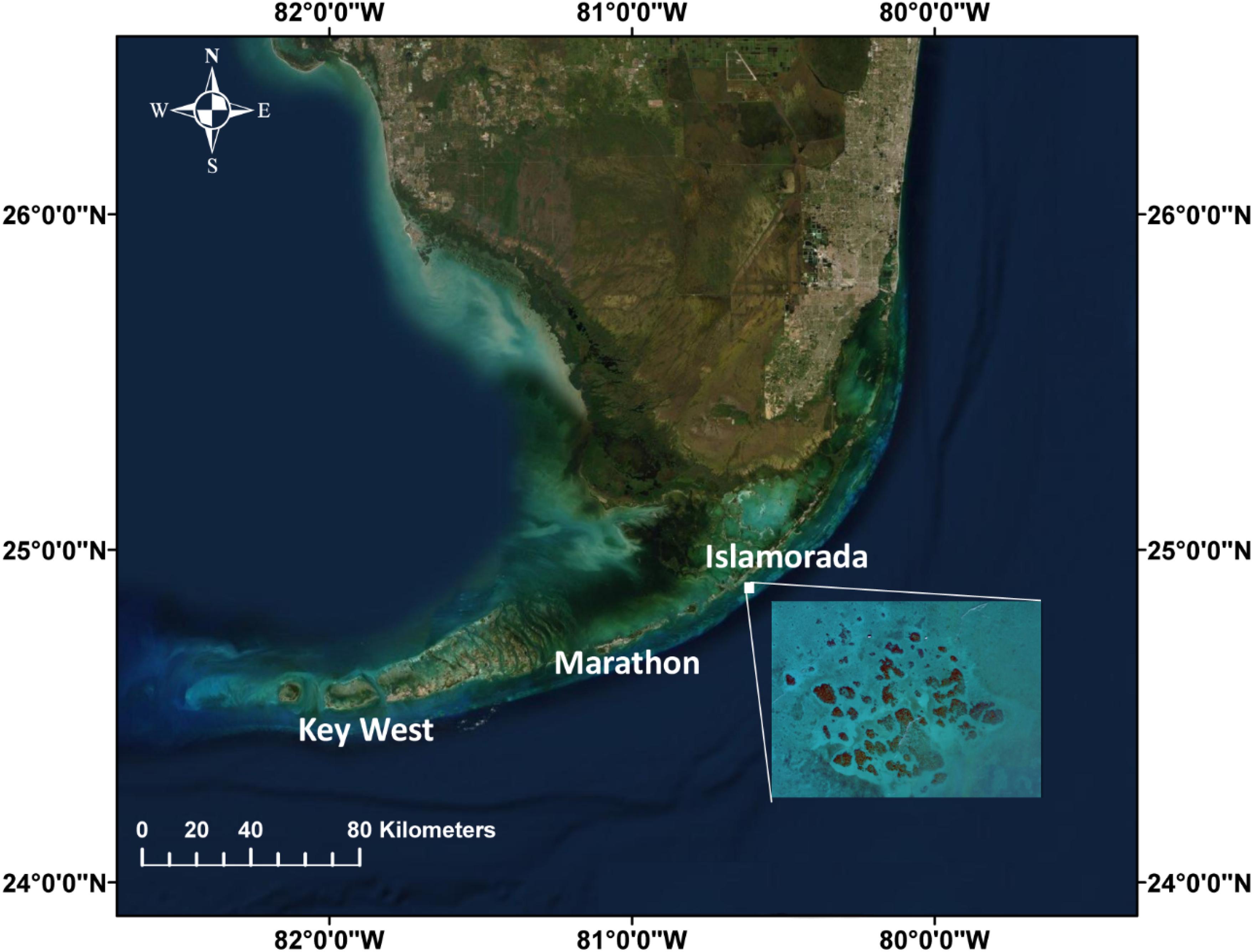
Figure 1. Florida Keys (created using ArcMap) and inserted satellite imagery obtained from Google Earth showing Cheeca Rocks.

3-D Model Reconstruction

The 3-D model in this study was created using the SfM photogrammetry software [Agisoft Metashape Pro 1.6, previously Photoscan AgiSoft MetaShape Professional (2020)] following a similar methodology outlined by Young et al. (2018), with a few additional steps that were found to enhance model quality (see Supplementary Information 2,3 for more details). The patch reef in Figure 2 was reconstructed from 2180 still images that were extracted from the video footage following the standard procedure set by Metashape. The final model was estimated to have a ground resolution of 0.278 mm/pixel and a reprojection error (i.e., root-mean square error) equal to 1.6 pixels with estimated accumulative error of 1.4 mm. For more information on 3-D model reconstruction see Supplementary Information 2.

FIGURE 2

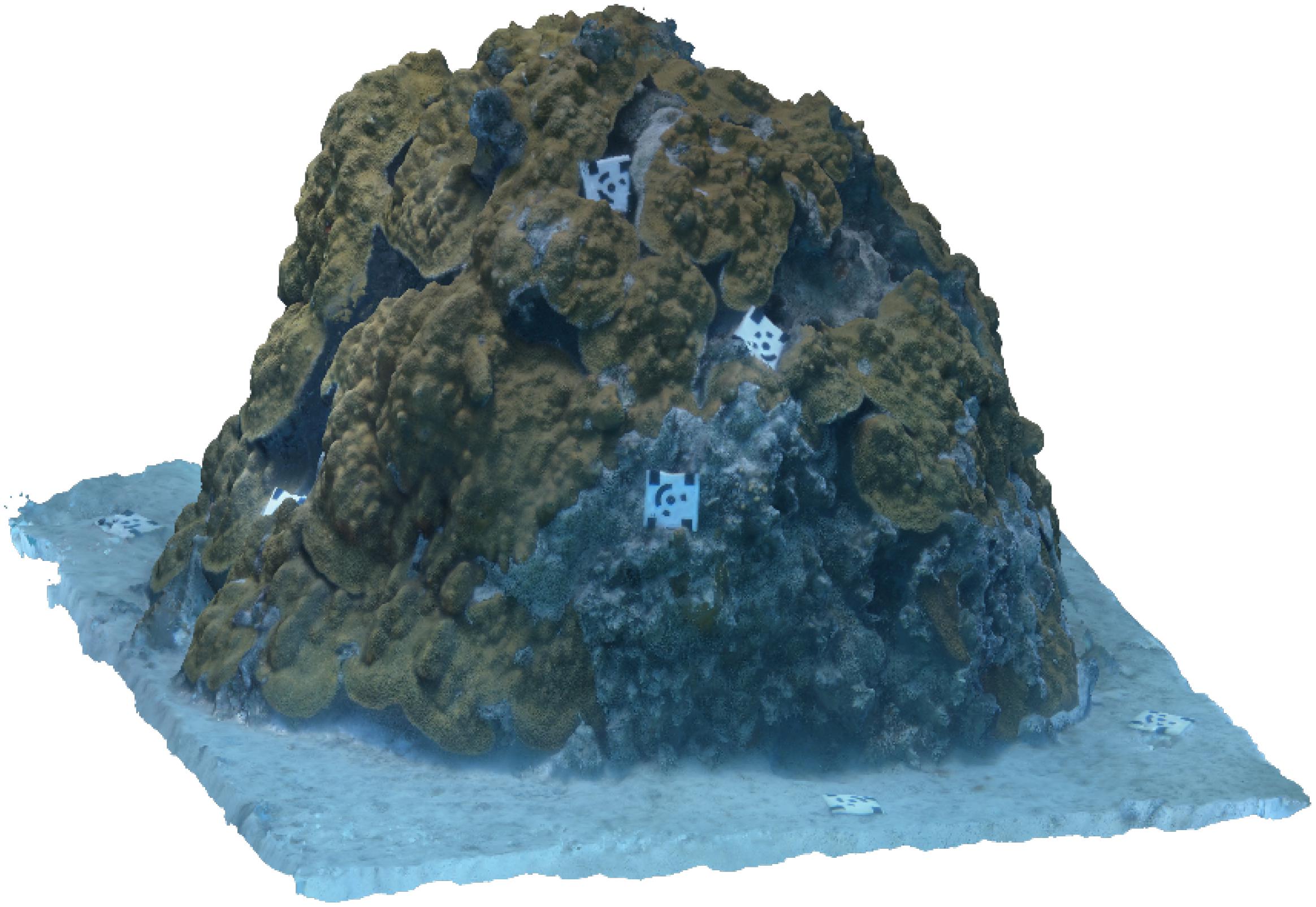
Figure 2. A textured mesh representing the example coral patch—which is roughly 1.5 m in diameter and 3 m in height—was reconstructed from still images extracted from video footage using Agisoft Metashape SfM photogrammetry software. The mesh consisted of 10 million faces and had an estimated accumulative error of 1.4 mm after providing absolute scale using the actual dimensions of the coded targets.

Deep Learning and Computer Vision Workflow

The 2180 still images used to reconstruct the 3-D model were the same ones used to train the FCN. However, before they could be used as training data they needed to be provided with the appropriate annotations. When training a deep learning semantic segmentation algorithm, every pixel in the image needs to be provided with a label denoting the class category to which it belongs (i.e., dense labels); as mentioned previously, this can be a time-consuming and expensive process. Even when using commercial image annotation software, creating dense labels manually can cost the annotator 20+ min per image. Thus, to reduce the burden this study designed a workflow that provided every still image in the dataset with dense labels while also minimizing the amount of work needed to be performed by the user (Figure 3).

FIGURE 3

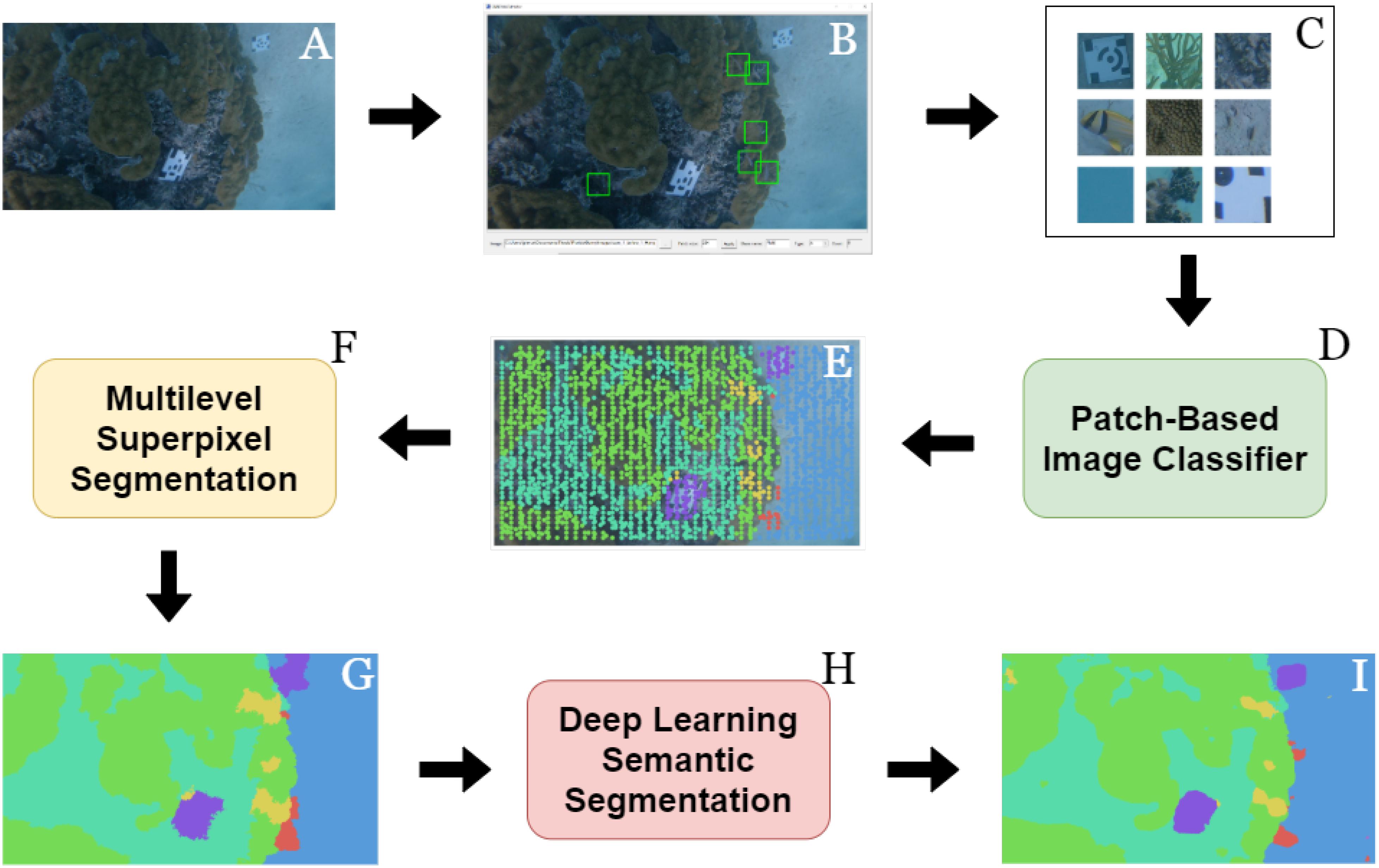
Figure 3. A diagram illustrating the workflow used to obtain dense labels for each image. Still images were extracted from the video footage (A) and imported into Rzhanov’s patch-extraction tool (B) where patches for each class category of interest were extracted (C). These patches and their corresponding labels were used to train a patch-based image classifier (D) that then provided numerous sparse labels to each image in the dataset (E). Using Fast-MSS (F), the sparse labels were converted into dense (G) and used as the pixel-wise labels necessary for training a deep learning semantic segmentation algorithm. (H) With a trained FCN, novel images collected from the same or similar habitats could then be provided with dense labels automatically (I) and without having to perform any of the previous steps (B–G).

Briefly summarized, the workflow started with the user manually creating sparse labels for each image (i.e., CPCe annotations) that were then used to train a CNN patch-based image classifier following a similar methodology outlined by others (Beijbom et al., 2012; Mahmood et al., 2016; Modasshir et al., 2018; Pierce et al., 2020). Once the classifier was sufficiently trained, it then served as an automatic annotator and was tasked with automatically providing all of the images in the dataset with numerous additional sparse labels. Once >0.01% of the pixels in an image were labeled, it was used with fast multilevel semantic segmentation (Fast-MSS), which converted them into dense labels automatically (Pierce et al., 2020). These dense labels and their corresponding images formed a dataset that were used to train a FCN capable of performing pixel-level classifications on unannotated images, thus eliminating the need to perform any of the previous steps in future studies when working in similar benthic habitats.

To quantitatively evaluate the accuracy of the results of these algorithms, 50 still images were first randomly sampled with replacement from the dataset and given an additional set of ground-truth dense labels that were created by hand using the commercial image annotation software LabelBox (Labelbox, 2020). These ground-truth dense labels served as a testing set to gauge the performance of the CNN patch-based image classifier, Fast-MSS, and the FCN.

The metrics used to evaluate accuracy include pixel accuracy (PA), mean pixel accuracy (mPA), weighted intersection-over-union (wIoU), and weighted dice coefficient (wDice). Weighted averages based on the frequency of each class were included because there existed a large imbalance between class categories, but no class was considered more important than any other. PA was computed by globally calculating the ratio of correctly classified pixels to the total number of pixels; this is identical to the overall classification accuracy and does not take into consideration class imbalances. The mPA calculates the global accuracy of each class individually and then averages them together so that each class contributes to the final score equally, regardless of class imbalances. PA and mPA were calculated by Eqs 1 and 2, respectively:

$$PA=\frac{TP+TN}{TP+FP+TN+FP}(1)$$

$$mPA=\frac{{\sum }_{i=1}^{n}P{A}_i}{N}(2)$$

where TP, TN, FP, and FN represent the True Positive, True Negative, False Positive and False Negative rates, respectively. Last are IoU (i.e., Jaccard index) and Dice (i.e., F1-Score, the harmonic mean between Recall and Precision), which are similarity coefficients commonly used for quantifying classification scores of semantic segmentation tasks (Eqs 3 and 5, respectively).

$$IoU=\frac{TP}{TP+FP+FN}(3)$$

$$\mathrm{\omega }IoU=\frac{{\sum }_{i=1}^{N}Io{U}_i*{\mathrm{\omega }}_i}{{\sum }_{i=1}^N{\mathrm{\omega }}_i}(4)$$

$$Dice=\frac{2*TP}{TP+FP+TN+FN}(5)$$

$$\mathrm{\omega }Dice=\frac{{\sum }_{i=1}^{N}Dic{e}_i*{\mathrm{\omega }}_i}{{\sum }_{i=1}^N{\mathrm{\omega }}_i}(6)$$

where the weight for each class w_i, was calculated as ratio of pixels per class over the total number of pixels in the test set.

Although there were multiple steps involved in this workflow, only the first step required manual effort from the user; the remaining steps were completed automatically using either the CNN patch-based image classifier, Fast-MSS, or the FCN. Thus, this workflow showcased that training data created through an almost entirely automatic process (as opposed to being done manually) could still produce a FCN that performs with acceptable classification scores useful in other applications.

Creating an Image-Patch Dataset

The workflow begins with the creation of a dataset from which a CNN patch-based image classifier could learn. Unlike a normal image classifier, a patch-based image classifier is trained on sub-images commonly referred to as “patches” that are cropped on individual class categories. A common method for creating an image-patch dataset is outlined in Beijbom et al. (2012); Mahmood et al. (2016), Modasshir et al. (2018), where patches are extracted and centered on top of the existing sparse labels that were created manually by a user with a point-based annotation software tool such as CPCe.

However, instead of going through the time-consuming process of creating CPCe annotations for each image, this study used a customized annotation software tool that was developed specifically for the purpose of extracting patches from still images. The patch-extractor is fast and provides an intuitive interface that allows the user to easily sample any part of the image, while archiving the location of extraction and assigned class label. Given the freedom to extract patches using a mouse or trackpad, a user can quickly create a highly representative dataset. Using this tool, roughly 10,000 patches with dimensions of 112 pixels by 112 pixels were extracted from the still images in the dataset, averaging approximately 50 patch extractions per minute.

Training a Convolutional Neural Network Patch-Based Image Classifier to Provide Additional Sparse Labels

This newly created dataset consisting of patches and their corresponding labels served as the training data for the CNN patch-based image classifier; as in Pierce et al. (2020), the classifier was first trained and then used to provide numerous additional sparse labels to each still image automatically.

Providing these additional sparse labels involved uniformly extracting patches with dimensions of 112 pixels × 112 pixels from an image following a grid formation. In total, approximately 2800 patches were sampled from each image in the dataset, representing potentially 2800 additional labels per image, or roughly 0.035% of the total number of pixels. Extracted patches were then passed to the trained classifier as input. The output for each patch was a corresponding vector representing the probability distribution of class categories to which the center-most pixel of the patch likely belonged. For each patch, the extracted location, the presumed class label, and the difference between the two highest probability distributions (i.e., top-1 and top-2 choices) were recorded.

The difference between the top two probabilities was considered the relative confidence level of the classifier when making the prediction. If the difference was small, the classifier was less confident about its top-1 choice (i.e., the presumed class label). By setting a confidence threshold value, sparse labels that the classifier was less certain about could be ignored. However, determining the ideal threshold involved trying different values and comparing the classification scores of the sparse labels predicted for the test images against the labels in the corresponding pixel indices of the manually created ground-truth dense labels (i.e., test set). As is discussed in the results section, the final threshold value that was chosen was a trade-off between the total number of labels that were accepted and their classifications scores.

With regards to efficiency, the CNN patch-based image classifier was able to assign roughly 200 sparse labels to an image per second, as opposed to the one annotation every 6 s that it cost users who used CPCe manually (Beijbom et al., 2015).

Converting Sparse Labels to Dense Using Fast-Multilevel Semantic Segmentation

The next step of the workflow converted the accepted sparse labels that were assigned to each image into dense using Fast-MSS (see Pierce et al., 2020 for more details on this method). As the name implies, this algorithm uses multiple iterations of an over-segmentation algorithm to partition the image into homogeneous regions called “super-pixels.” The class category of existing sparse labels for the image are then propagated to neighboring pixels located within the same super-pixel, assigning them labels automatically. This process is repeated for multiple iterations, and then joins all of the labels together to create a set of dense labels for the image representing the pixel-level classifications for each observed functional group (see Figure 3G).

For this dataset, the first and last number of super-pixels to partition each image was 5000 and 300, respectively, and across 30 iterations. Each image was down-sampled by reducing the height and width by a factor of six after confirming that a reduction in the input image’s dimensions could decrease the time required to create the dense labels without negatively affecting the classification scores (see Table 1). Dense labels were then up-sampled using nearest neighbor interpolation so they matched the image’s original dimensions, a requirement for deep learning model training.

TABLE 1

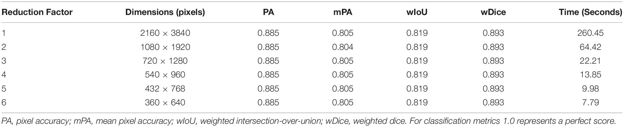
Table 1. The effect of reducing an input image’s dimensions on the output of Fast-MSS.

Training Fully Convolutional Networks on Fast-Multilevel Semantic Segmentation Dense Labels

Although the dense labels created by Fast-MSS could have been used to classify the 3-D reconstructed model directly, they were also used as training data with a deep learning semantic segmentation algorithm to produce a FCN. The major advantage of a FCN is its ability to generalize to images collected from domains that are similar to those on which it was trained. A researcher could obtain dense labels from an FCN given images collected from the same or similar habitats that it was previously trained on without having to perform any of the previous steps in the workflow (steps B-G). Thus, the objective of this workflow was not just to obtain a set of dense labels for every still image, but rather to acquire a deep learning semantic segmentation model that could create dense labels automatically for datasets collected in the future.

This study experimented with five different FCNs to understand how the size of the network affected the classification accuracy. Each FCN used an encoder from the EfficientNet series (Tan and Le, 2019) and was used to create an additional set of dense labels for every image in the dataset; these and the set created by Fast-MSS were validated and compared against the ground-truth dense labels that were manually created for the test set.

Class Categories

Of the different organisms, substrate types, and objects present in the video footage data, seven class categories were formed. Four of these were biological (“Branching Soft and Hard Coral,” “Fish,” “Massive Coral,” and “Algae”) and consisted of multiple species, one encompassed all of the potential substrate types (“Substrate”), another was used to denote the coded targets (“Target”), and lastly was the class used to represent the background (“Water,” Figure 4). The first five class categories served as functional groups to demonstrate the ability to calculate community composition in both 2-D images and 3-D models, but alternative functional groups, genuses, or even species could be chosen for different purposes.

FIGURE 4

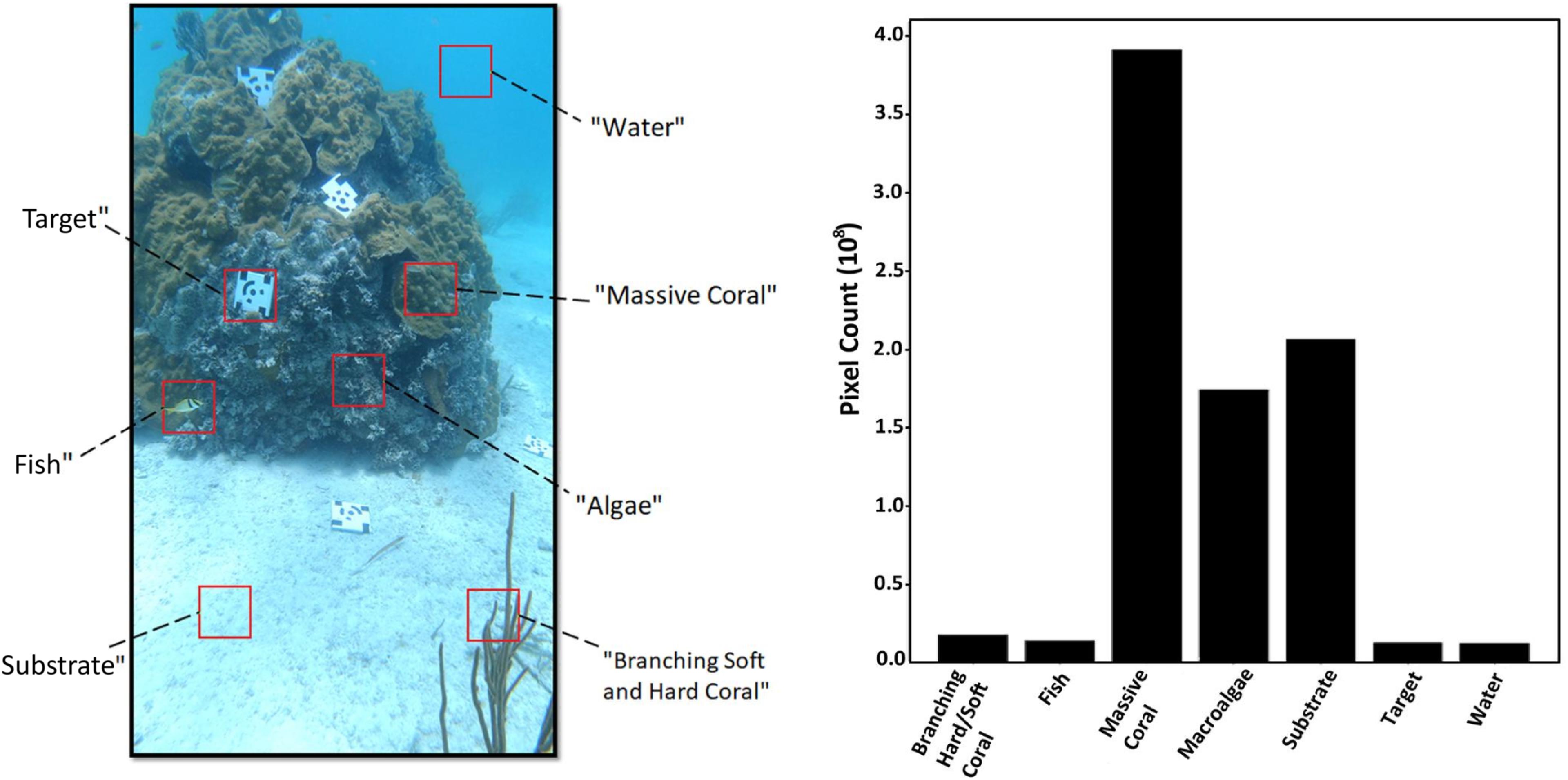
Figure 4. A still image (2160 pixels × 3840 pixels) extracted from the video footage showcasing the class categories used in this study (left), and the distribution of each class category based on their pixel count calculated from the 50 ground-truth dense labels within the testing set (right).

The majority of the still images in the dataset were made up of pixels that belonged to massive corals (Orbicella faveolata, Orbicella annularis, and Porites astreoides), followed by different types of substrate (sand, rubble). The third most represented class category was “Algae,” which contained some crustose coralline algae (CCA) and filamentous turf algae, but primarily Halimeda spp., which was found in abundance in crevices between coral colonies. The “Branching Soft and Hard Coral” class was comprised of various types of branching morphologies including octocorals (e.g., sea pens, sea fans) and fire coral (Millepora alcicornis), and the “Fish” class category incorporated all individuals with no distinction made among species. To ensure the coded targets would not be associated with one of the functional groups, a class was created for it. Lastly “Water” served as the background class meant to represent the pixels in an image where there was nothing visible as a result of light attenuation through the water column.

These seven class categories could be found in the still images, but only “Branching Soft and Hard Coral,”, “Massive Coral,” “Algae,” “Substrate,” and “Target” were included in the 3-D model because SfM photogrammetry is only capable of reconstructing objects that are static within the source images. Thus “Fish” and “Water” were excluded from the model.

Model Training

The CNN patch-based image classifier that was used to provide numerous additional sparse labels to each image as described in the workflow used the EfficientNet-B0 architecture. Instead of using the typical “ImageNet” weights, the classifier was initialized with the “Noisy-Student” weights, which were learned using a semi-supervised training scheme that outperformed the former (Xie et al., 2020). This encoder was followed by a max pooling operation, a dropout layer (80%), and finally a single fully connected layer with seven output nodes (one for each of the class categories). Patches were resized to 224 pixels × 224 pixels and fed to the model as training data after heavy augmentation techniques were applied using the ImgAug (Jung, 2019) library, and normalized to have pixel values between 0 and 1.

The task is considered a multi-categorical classification, therefore the network used a softmax activation function resulting in an output representing the probability distribution of each potential class category. The batch size was set to 32 as this was the largest amount possible given the network architecture, the size of the image patches, and the amount of memory that could be allocated by the GPU being used. The model was trained on 10,000 image patches that were randomly split into a training (90%) and validation (10%) set for 25 epochs; the final model was evaluated using the test set that consisted of 50 manually created ground-truth dense labels (see Table 2).

TABLE 2

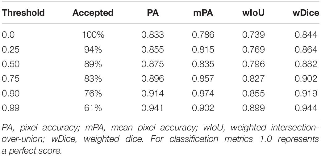
Table 2. Classification scores for the CNN patch-based image classifier compared against ground-truth.

During training the error between the actual and predicted output was calculated using the categorical-cross entropy loss function. Parameters throughout the network were adjusted using the Adam optimizer with an initial learning rate of 10^–4. During training the learning rate was reduced by a factor of 0.5 for every three epochs in which the validation loss failed to decrease, and the weights from the epoch with the lowest validation loss were archived.

For the task of semantic segmentation this study experimented with five different FCNs, all of which used the U-Net architecture and were equipped with one of the five smallest encoders within the EfficientNet family (i.e., B0 through B4, see Supplementary Information 4 for more information). All models were implemented in Python using the Segmentation Models library (Yakubovskiy, 2019).

When training the FCNs, the error was calculated using the soft-Jaccard loss function, which acted as a differentiable proxy that attempted to maximize the Intersection-over-Union metric (Berman et al., 2018). Parameters were updated via backpropagation using the Adam optimizer with an initial learning rate of 10^–4, which decreased using the same settings as described before. After 20 epochs, the weights from the epoch with the lowest validation loss were archived. All deep learning models were trained on a PC equipped with a NVIDIA GTX 1080 Ti GPU and an Intel i7-8700 CPU, using the Keras deep learning framework and the Tensorflow numerical computational library; for more information see Supplementary Information 4.

3-D Model Classification

Following the training process, Fast-MSS and the five FCNs experimented with were each used to create a different set of dense labels for each of the 2180 images in the dataset. With each respective set of dense labels, a separate classified 3-D model was created, thus allowing the comparison between each of the five FCN encoders (i.e., EfficientNet B0–B4) and Fast-MSS. The technique to assign semantic labels to the 3-D model was straightforward and was done almost entirely in Agisoft Metashape (see Figure 5).

FIGURE 5

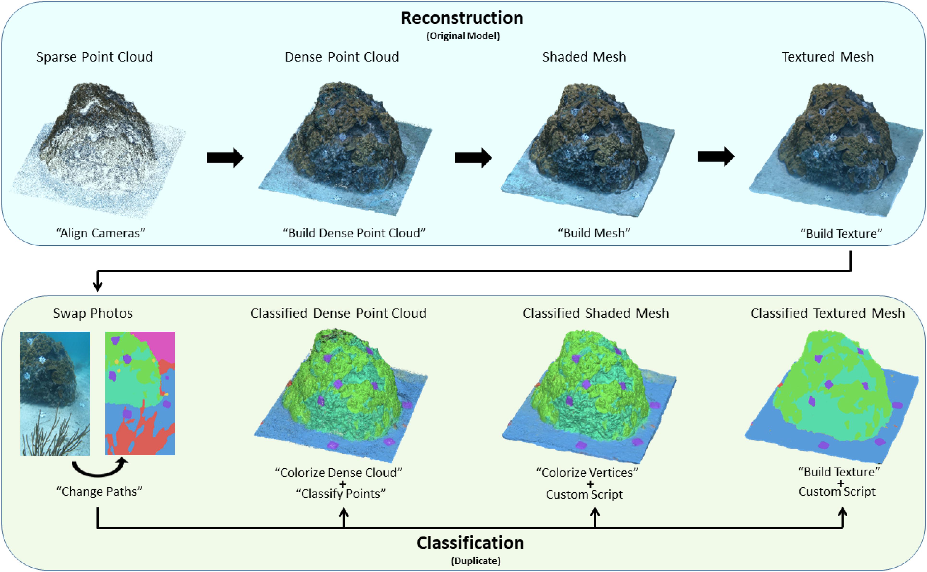
Figure 5. A diagram showing step-by-step which tools in Agisoft Metashape were used to reconstruct the 3-D model, followed by how semantic labels were provided to it. Once the source images are swapped with their corresponding dense labels, the classified point cloud, shaded mesh, and textured mesh can be created independently of one another and is not a sequential process like the reconstruction.

Once the textured mesh for the 3-D model was created, the entire project was duplicated and a second textured mesh was created, but using dense labels as source images instead of the originals. The process involved first swapping the original images with their corresponding dense labels using the “Change Paths” tool. Next, the “Build Texture” tool was used with the “Source data” parameter set to “Images,” the “Blending” mode was disabled, and the “Keep UV” parameter was kept active. By disabling blending we could ensure that the discrete categorical values representing each class in the dense labels would not be accidentally averaged or “bleed” along the borders of neighboring semantic groups in the resulting classified textured mesh. With the “Keep UV” parameter kept to active, the texture for the classified 3-D model used the same texture coordinates as those that were created when reconstructing the original textured model; this ensured that the predictions from the dense labels used the same UV mapping from image-space to model-space as the pixels in the original images. Once completed, the classified textured mesh was identical to the original in appearance, but with textures that were mapped from the set of dense labels that were used as source images instead of the originals (see Figure 6).

FIGURE 6

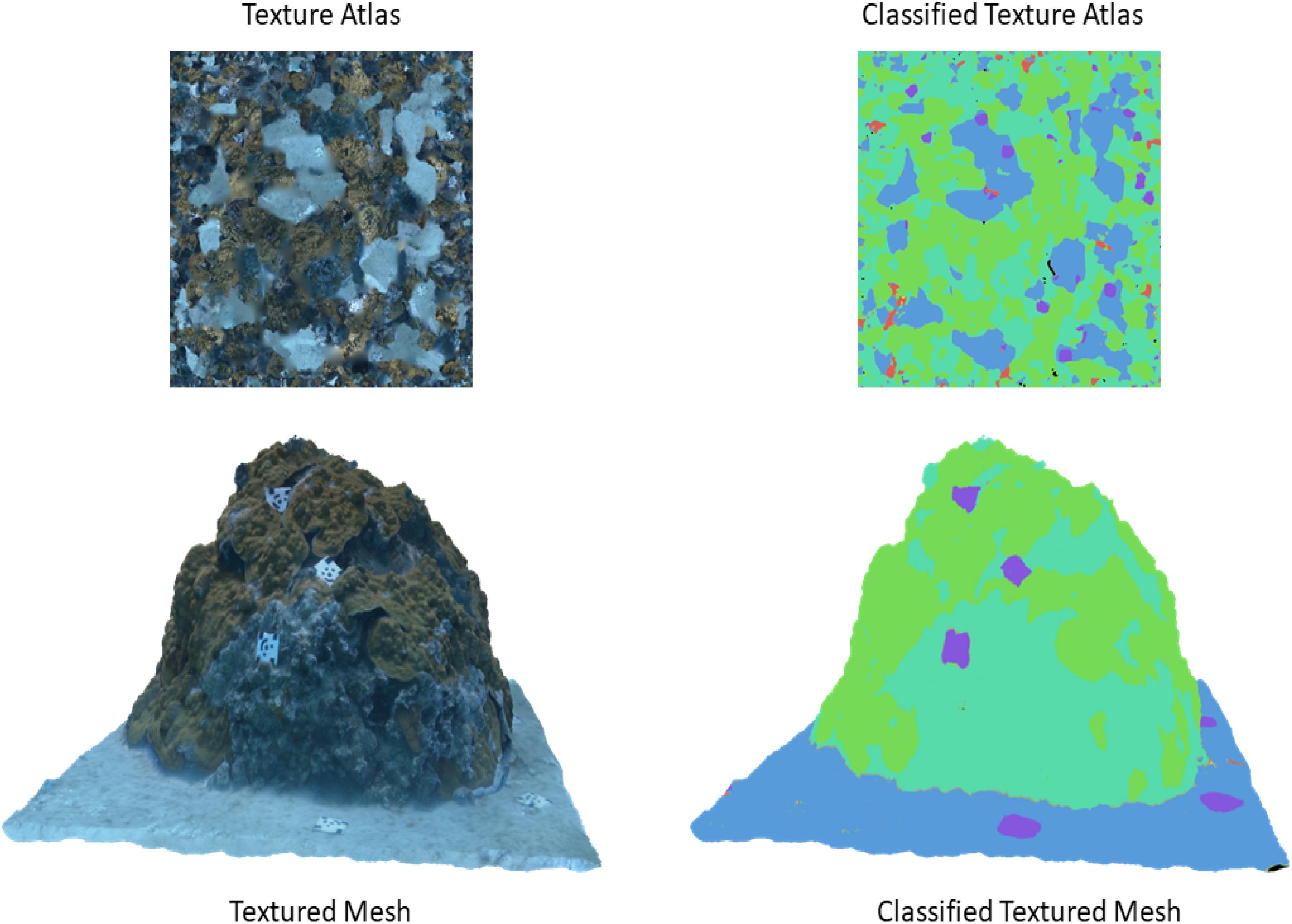
Figure 6. Comparison between the textured mesh and its corresponding atlas (left) against the classified version of the mesh and its corresponding atlas after being corrected using the custom post-processing script (right).

A classified shaded mesh and dense point cloud were then created using the “Colorize Vertices” and “Colorize Dense Cloud” tools, respectively. These tools worked similarly in that they mapped the color components from the pixel indices found in the source images (in this case, the dense labels) to their corresponding elements or points within the shaded mesh or dense cloud. However, the blending mode could not be disabled in either “Colorize Vertices” or “Colorize Dense Cloud” resulting in some of the elements or points having color components with values that were averaged together and were not within the set of discrete values denoting one of the class categories. To correct this issue and to obtain discretely classified points in the dense point cloud, we used the “Classify Points” tool to first select points based on a range of similar color component values, and then reclassified them to the correct class category. However, because version 1.6 of Metashape Pro does not offer a “Classify Vertices” tool, the color component values for each vertex of the shaded mesh were corrected in the same way but done outside of Metashape using a custom Python script (see Supplementary Information 5).

Validation for the classified model was obtained by comparing the classified texture atlas (Figure 6) with a manually annotated texture atlas (not shown) that served as ground-truth. Accuracy assessments of the original and classified textured mesh were completed using similarity metrics including PA, mPA, wIoU, and wDice when compared as 2-D images. The original and the classified textured mesh were first exported as 2-D images (i.e., texture atlases) using the “Export Texture” tool, and then the former was made into a “ground-truth texture atlas” by manually providing it with semantic labels using the image annotation software tool LabelBox (Labelbox, 2020). Similar to annotation of a 2-D image, the pixel indices in the ground-truth texture atlas were assigned labels denoting the class category they were thought to belong to by a trained annotator. However, not all textures could be discerned by the annotator as some were either too small, or simply did not resemble any of the class categories when represented in the texture atlas. In such cases, the annotator assigned labels only to the pixel indices they were able to identify, resulting in a ground-truth texture atlas (4096 pixels by 4096 pixels) where ∼88% of the pixels were provided with semantic labels.

Experiments

This study validated the results of the CNN patch-based image classifier and its ability to produce sparse labels, the dense labels that were created by Fast-MSS, the predictions made by the five FCNs experimented with, and the classification accuracy of the 3-D classified models. To calculate classification scores, the sparse labels predicted by the CNN patch-based image classifier for each image in the test set were compared to the labels in the corresponding pixel indices of the ground-truth dense labels that were made manually using LabelBox (Labelbox, 2020). Similarly, the dense labels created by Fast-MSS and the FCNs for each image in the test set were also compared to the same ground-truth dense labels. Lastly, each classified 3-D model was evaluated by comparing the semantic labels in the exported 2-D image (i.e., classified texture atlas) of each 3-D model against the labels in the ground-truth texture atlas that was created manually by a trained annotator.

Results

First, we present the results of how the CNN patch-based image classifier’s performance changed as a function of the confidence threshold value used. The confidence score was used to filter sparse labels that were more likely to have been misclassified.

Table 2 is the inverse relationship between the confidence threshold value chosen and the percentage of sparse labels accepted: as the threshold value increases, the model becomes more conservative with its predictions (Figure 7). This also created a direct relationship between the threshold value and the classification scores, because again, as more of the labels the model was not confident about were rejected, the overall classification accuracy of the remaining labels was likely to increase. Based on these results, 0.50 was chosen as the confidence threshold value for the remainder of the workflow as it was deemed to produce results that balanced this trade-off.

FIGURE 7

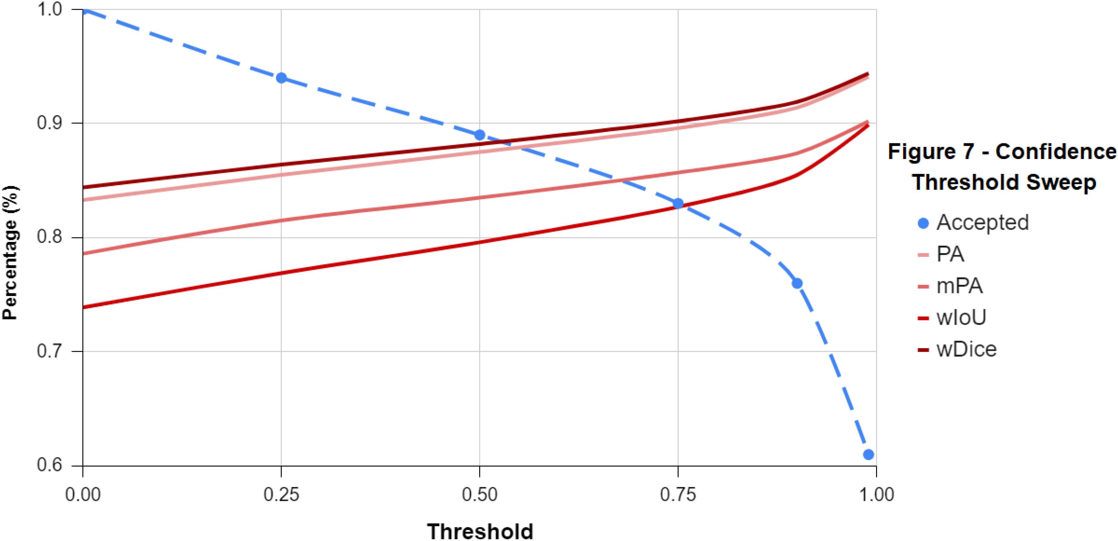
Figure 7. A line-graph displaying the inverse relationship between the confidence threshold value and the classification scores of the sparse labels accepted. As the threshold value increases and becomes more conservative along the x-axis, more of the sparse labels the classifier was unsure about were rejected.

Table 3 shows that the dense labels produced by Fast-MSS had classification scores that were slightly less than those created by any of the FCNs, except for B2, which produced the lowest scores among the FCNs (Table 3). The differences in performance were marginal. With regards to speed, all FCNs performed substantially faster than Fast-MSS, whose recorded time also included the time required by the CNN patch-based image classifier to first predict sparse labels for the input image. Even when the original input image with dimensions of 736 pixels by 1280 pixels was reduced by a factor of 6×, the CNN patch-based image classifier/Fast-MSS combo produced results in 22.6 s, which is still 10× slower than the slowest FCN.

TABLE 3

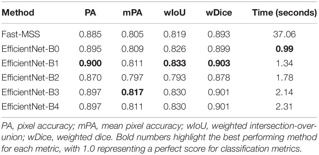
Table 3. Classification scores of each method for producing dense labels compared against ground-truth.

A key takeaway from Table 3 is that even though the FCNs were trained on the dense labels produced by Fast-MSS, all but B2 achieved higher classification scores. This suggests that as a deep learning algorithm, a FCN has the potential to develop a better understanding of which features are associated with each class category by learning from all of the images collectively throughout the training process.

Last are the results for the classified 3-D model (Table 4), which shows that the overall classification scores followed the same general trend that can be seen in Table 3. The classified texture atlas that used the dense labels produced by Fast-MSS as the source images had scores for PA, wIoU, and wDice that were slightly less than those created by any of the FCNs; the FCNs were equally good with no clear indication that one outperformed another.

TABLE 4

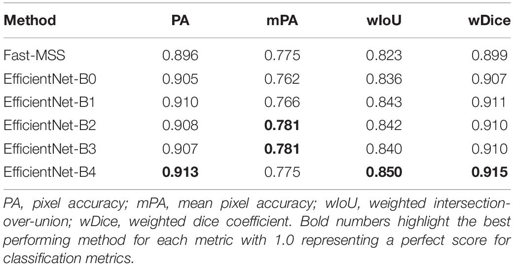
Table 4. Classification scores of 3-D models represented as texture atlases compared against ground-truth.

Table 4 shows that the difference in scores between each 3-D model is not substantial, though the fact that they closely resemble the scores seen in Table 3 suggests three things. The first is that Agisoft Metashape is able to map each semantic label from the dense labels to create a 3-D classified model with a high level of accuracy. Secondly, the classification scores of the 3-D models appear to be largely dependent on the classification scores of the dense labels that were used as source images; this reinforces what was already assumed to be true and also provides positive validation for this technique for creating 3-D classified models. Finally, the results suggest that the non-conventional ground-truth texture atlas that was created is of similar quality when compared to the more conventional ground-truth dense labels that were created for the images in the test set. This provides validation for this method of evaluating the classification scores of the 3-D model directly, which could prove useful in future studies.

Though the scores between Tables 3, 4 are similar, there is a pattern of a 1 to 2-point increase for PA, wIoU, and wDice, which may be caused by the blending of color components that occurs during the building of a textured mesh. For each individual element within the 3-D mesh, there are multiple pixels found within different source images that all correspond to it, but from different vantage points. When creating the textured mesh with the blending mode set to either “mosaic,” each element is assigned a color based on the weighted average of the color components from the pixels that it corresponds to (Metashape, see Supplementary Information 3). Thus, by using “mosaic,” the blending of source images—in this case, the dense labels—may serve as a weighted average ensemble that contributes to slightly higher classification scores (Hopkinson et al., 2020).

These results provide evidence that this method can accurately assign semantic labels from source images to a 3-D model, and that resulting classification accuracy of the classified textured mesh is a function of the reconstruction error of the original model, as well as the classification scores of the method used to produce the dense labels (i.e., Fast-MSS and the FCNs). Although the classified textured mesh is not typically used in spatial analyses, this study showed that it can serve as a useful proxy for validating the accuracy of the classified shaded mesh and dense point cloud, which often are. Since the elements that make up the textured mesh store both the texture coordinates and the color components, it stands to reason that all three model types share similar classification scores (Figure 8).

FIGURE 8

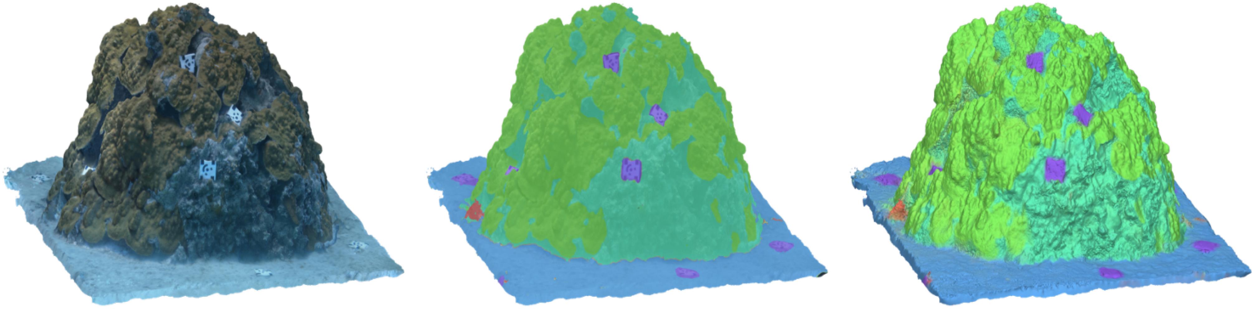
Figure 8. A side-by-side comparison between the textured mesh (left), the classified textured mesh with 40% transparency (center), and the classified shaded mesh (right). The classified textured mesh was used as a method for validating the classification results of the classified shaded mesh and dense point cloud (not shown), which can be used in spatial analyses.

Discussion

Coral reefs are complex 3-dimensional structures that promote the assemblage of diverse groups of organisms by creating spaces for the establishment of sessile sponges, ascidians, hydroids and bryozoans, and by providing shelter for prey seeking refuge from predation. Although 2-D images collected through benthic quadrat surveys are routinely used to evaluate community composition, this form of representation fails to capture the changes that occur to a coral reef when considering the 3-dimensional structure, arguably one of its most important attributes.

Generally, the 3-D structure of a reef is studied through the use of metrics such as rugosity and fractal dimensions to quantify specific aspects of the architecture (Young et al., 2018). These metrics are then correlated with important ecosystem functions such as species richness, abundance and assemblage. Rugosity—the oldest and most prevalent metric used in these types of studies—is obtained by using a technique called the “tape-and-chain” method, which requires divers to physically lay out a chain to measure the surface of a coral colony or an entire reef in situ (Risk, 1972). SfM algorithms are designed for non-technical users and many ecologists have begun favoring photogrammetry over more traditional techniques. By doing so researchers are able to obtain a highly precise (<2 mm error) digital representation of the physical habitat from which a number of spatial analyses can be performed (Ferrari et al., 2016; Young et al., 2018).

Due to the wide reaching applications of SfM within this domain, we developed a mostly automated workflow for classifying 3-D photogrammetric models. This workflow will provide a more efficient method for monitoring changes in structural complexity and community composition in both marine and terrestrial environments. Unlike the method described in Hopkinson et al. (2020) that performs image classification, our method performs semantic segmentation. The critical distinction being that instead of performing image classification multiple times for each individual element of the model one-by-one, our method only needs to classify or provide each image used in the reconstruction process with a corresponding set of dense labels once. Then, using the re-projection matrices created during the photo alignment phase these dense labels can be accurately projected onto the point cloud and mesh using the same mechanism (i.e., UV coordinates) that provided the original model with its color component values. This results in the accuracy of the 3-D classified model being largely dependent on both the accuracy dense labels (i.e., Fast-MSS, FCNs) and the quality of the 3-D model itself (see Tables 3, 4). It also means that this method scales linearly and can be used to provide semantic labels to a 3-D model regardless of its size or resolution.

However, to obtain labels for a 3-D model each image used in the reconstruction process must first be provided with a corresponding set of dense labels. This can of course be done manually by using an image annotation tool (e.g., LabelBox Labelbox, 2020) or using an AI-assisted labeling tool such as TAGLab, though depending on the number of images used to create the 3-D model this could require a significant amount of time, and thus might not always be feasible for a study. In our workflow we described how to obtain dense labels for an image automatically by using the associated sparse labels with Fast-MSS. Due to the ubiquitousness of CPCe annotations within the field of benthic ecology, their inclusion in the workflow makes our method more accessible and easier to emulate in other studies. However, we do acknowledge that the benthic quadrat survey images that CPCe annotations are typically made for are not usually the same images used with SfM algorithms to reconstruct a 3-D model. In the scenarios where sparse labels have not already been created for the images we recommend using an annotation tool such as the patch-extractor tool or CoralNet (Beijbom et al., 2015) to create them, both of which are much faster and less taxing on the user compared to CPCe. Regardless of the method chosen, once sparse labels have been created they can be converted into dense labels automatically using Fast-MSS and used to either train a deep learning semantic segmentation algorithm, or classify the 3-D model directly (both of which were shown to be capable of achieving high levels of accuracy, see Table 4).

Our method can be used to efficiently and accurately segment the 3-D structure into specific class categories (e.g., species, genuses, functional groups). Hence, this study moves beyond 2-dimensional analyses and begins to quantify 3-D coverage statistics allowing for greater insight into the complex spatial relationships between groups within a reef community. This ability to classify the individual elements of a 3-D model also allows for metrics of structural complexity to be resolved from the model-scale down to the functional or even species-scale. This could have a significant impact on the understanding of species-specific effects of coral restoration on biodiversity or ecosystem functions. Coral reef communities are undergoing rapid changes in species compositions including shifts from hard to soft corals (Inoue et al., 2013), or corals to macro-algae (McManus and Polsenberg, 2004). There is also a growing effort to restore reefs by outplanting corals that have dissimilar morphologies, which may differentially contribute to reef complexity and architecture. Consequently, it will be important to have an efficient, reliable and repeatable method that quantifies the amount of structural complexity that each individual functional group contributes to the overall reef complexity.

The method outlined here was applied to a tropical coral reef, though it is agnostic to the domain and would be suitable for many other ecosystems including deep sea coral communities, oyster reefs, intertidal zones, and even some terrestrial environments. As discussed previously, the ability to apply this method—regardless of the domain—is dependent on the quality of the 3-D reconstructed model itself, and the accuracy of the dense labels produced, whether they were made manually, by Fast-MSS, or a deep learning model. If both are independently accurate, the predictions projected from image-space to model-space should be proportionally accurate. However, if the dense labels associated with each image used in the reconstruction are of low accuracy, the labels for the 3-D classified model will also be of low accuracy regardless of the quality of the 3-D reconstructed model. Alternatively, if the quality of the 3-D reconstructed model is poor due to misalignment, occlusions, a noisy point cloud, etc., spatial statistics calculated from the 3-D classified model may not be accurate even when the dense labels are. Data collection and the reconstruction of 3D models for other habitats will depend on topographic features (e.g., vertical relief), currents and/or surge (in marine environments) as both will affect the number of images needed to acquire an accurate model. To ensure quality results, 3-D reconstructed models should be created from mostly static scenes using a high-resolution camera, and with ground control points (i.e., coded targets) strategically placed around areas of interest; for more information on performing SfM in underwater scenes in particular, we refer interested readers to the Supplementary Information section and (Ferrari et al., 2016; Young et al., 2018; Bayley and Mogg, 2020; Hopkinson et al., 2020).

This study represents a step toward fully automated assessments and monitoring systems for coral reefs. It is hoped that the techniques outlined here can provide some assistance in understanding how the changes that are occurring are affecting benthic habitats, and serve as a stepping stone for more advanced techniques to build off of in the near future. To ensure repeatability and ease-of-use, we have open-sourced our code and provided instructions for its use, which are located in our Github repository.

Data Availability Statement

The datasets presented in this study can be found in online repositories. The names of the repository/repositories and accession number(s) can be found below: www.github.com/jorda nmakesmaps/3D-Model-Classification.

Author Contributions

JP and JD: methodology, investigation, data wrangling, and project administration. JP, JD, MB, KL, and YR: formal analysis and writing. JP, JD, and MB: resources and data collection. JD, YR, and KL: supervision. JD and MB: funding acquisition. All authors contributed to the conceptualization, writing, review, and editing of the manuscript, and read and agreed to the published version of the manuscript.

Funding

Funding for this study was provided by NOAA grant/award number NA15NOS4000200.

Conflict of Interest

The authors declare that the research was conducted in the absence of any commercial or financial relationships that could be construed as a potential conflict of interest.

Publisher’s Note

All claims expressed in this article are solely those of the authors and do not necessarily represent those of their affiliated organizations, or those of the publisher, the editors and the reviewers. Any product that may be evaluated in this article, or claim that may be made by its manufacturer, is not guaranteed or endorsed by the publisher.

Acknowledgments

We would like to thank the Butler Lab for their help with data collection, and our reviewers for their time, feedback, and insightful questions.

Supplementary Material

The Supplementary Material for this article can be found online at: https://www.frontiersin.org/articles/10.3389/fmars.2021.706674/full#supplementary-material

References

AgiSoft MetaShape Professional (2020). AgiSoft MetaShape Professional (Version 1.6) (Software). Available online at: http://www.agisoft.com/downloads/installer/ (accessed June 1, 2019).

Google Scholar

Bayley, D. T., and Mogg, A. O. (2020). A protocol for the large-scale analysis of reefs using structure from motion photogrammetry. Methods Ecol. Evolut. 11, 1410–1420. doi: 10.1111/2041-210x.13476

CrossRef Full Text | Google Scholar

Beijbom, O., Edmunds, P. J., Kline, D. I., Mitchell, B. G., and Kriegman, D. (2012). “Automated annotation of coral reef survey images,” in 2012 IEEE Conference on Computer Vision and Pattern Recognition, (Rhode Island, RI: CVPR), doi: 10.1109/cvpr.2012.6247798

CrossRef Full Text | Google Scholar

Beijbom, O., Edmunds, P. J., Roelfsema, C., Smith, J., Kline, D. I., Neal, B. P., et al. (2015). Towards Automated Annotation of Benthic Survey Images: Variability of Human Experts and Operational Modes of Automation. PLoS One 10:0130312. doi: 10.1371/journal.pone.0130312

PubMed Abstract | CrossRef Full Text | Google Scholar

Berman, M., Triki, A. R., and Blaschko, M. B. (2018). “The Lovasz-Softmax Loss: A Tractable Surrogate for the Optimization of the Intersection-Over-Union Measure in Neural Networks,” in 2018 IEEE/CVF Conference on Computer Vision and Pattern Recognition, (Utah: CVPR), doi: 10.1109/cvpr.2018.00464

CrossRef Full Text | Google Scholar

Burke, L. M. (2012). Reefs at risk revisited. Washington, D.C.: World Resources Institute.

Google Scholar

Burns, J., Delparte, D., Kapono, L., Belt, M., Gates, R., and Takabayashi, M. (2016). Assessing the impact of acute disturbances on the structure and composition of a coral community using innovative 3D reconstruction techniques. Methods Oceanogr. 15-16, 49–59. doi: 10.1016/j.mio.2016.04.001

CrossRef Full Text | Google Scholar

Cesar, H., Burke, L., and Pet-Soede, L. (2003). “The Economics of Worldwide Coral Reef Degradation,” in International Coral Reef Action Network, (Arnhem: CEEC).

Google Scholar

De’ath, G., Fabricius, K. E., Sweatman, H., and Puotinen, M. (2012). The 27-year decline of coral cover on the Great Barrier reef and its causes. Proc. Natl. Acad. Sci. 109, 17995–17999. doi: 10.1073/pnas.1208909109

PubMed Abstract | CrossRef Full Text | Google Scholar

Ferrari, R., McKinnon, D., He, H., Smith, R. N., Corke, P., and Gonzalez-Rivero, M. (2016). Quantifying Multiscale Habitat Structural Complexity: A Cost-Effective Framework for Underwater 3D Modelling. Rem. Sens. 8:113.

Google Scholar

Harborne, A. R., Mumby, P. J., and Ferrari, R. (2011). The effectiveness of different meso-scale rugosity metrics for predicting intra-habitat variation in coral-reef fish assemblages. Environ. Biol. Fishes 94, 431–442. doi: 10.1007/s10641-011-9956-2

CrossRef Full Text | Google Scholar

Hopkinson, B. M., King, A. C., Owen, D. P., Johnson-Roberson, M., Long, M. H., and Bhandarkar, S. M. (2020). Automated classification of three-dimensional reconstructions of coral reefs using convolutional neural networks. PLoS One 15:0230671. doi: 10.1371/journal.pone.0230671

PubMed Abstract | CrossRef Full Text | Google Scholar

Inoue, S., Kayanne, H., Yamamoto, S., and Kurihara, H. (2013). Spatial community shift from hard to soft corals in acidified water. Nat. Clim. Change 3, 683–687. doi: 10.1038/nclimate1855

CrossRef Full Text | Google Scholar

Jokiel, P. L., Rodgers, K. S., Brown, E. K., Kenyon, J. C., Aeby, G., Smith, W. R., et al. (2015). Comparison of methods used to estimate coral cover in the Hawaiian Islands. PeerJ 3:954. doi: 10.7717/peerj.954

PubMed Abstract | CrossRef Full Text | Google Scholar

Jung (2019). ImgAug. GitHub Repository. San Francisco, CA: github. Available online at: https://github.com/aleju/imgaug (accessed February 1, 2019).

Google Scholar

Kohler, K. E., and Gill, S. M. (2006). Coral Point Count with Excel extensions (CPCe): A Visual Basic program for the determination of coral and substrate coverage using random point count methodology. Comput. Geosci. 32, 1259–1269. doi: 10.1016/j.cageo.2005.11.009

CrossRef Full Text | Google Scholar

Labelbox (2020). Get to production AI faster. San Francisco, CA: Labelbox. Available online at: https://labelbox.com (accessed March 15, 2019).

Google Scholar

Mahmood, A., Bennamoun, M., An, S., Sohel, F., Boussaid, F., Hovey, R., et al. (2016). “Coral classification with hybrid feature representations,” in 2016 IEEE International Conference on Image Processing (ICIP), (Arizona, ARI: ICIP), doi: 10.1109/icip.2016.7532411

CrossRef Full Text | Google Scholar

McManus, J. W., and Polsenberg, J. F. (2004). Coral–algal phase shifts on Coral reefs: Ecological and environmental aspects. Prog. Oceanogr. 60, 263–279. doi: 10.1016/j.pocean.2004.02.014

CrossRef Full Text | Google Scholar

Modasshir, M., Li, A. Q., and Rekleitis, I. (2018). “MDNet: Multi-Patch Dense Network for Coral Classification,” in OCEANS 2018 MTS/IEEE Charleston, (Charleston, SC: MTS), doi: 10.1109/oceans.2018.8604478

CrossRef Full Text | Google Scholar

Nyström, M., Folke, C., and Moberg, F. (2000). Coral reef disturbance and resilience in a human-dominated environment. Trends Ecol. Evolut. 15, 413–417. doi: 10.1016/s0169-5347(00)01948-0

CrossRef Full Text | Google Scholar

Pierce, J., Rzhanov, Y., Lowell, L., and Dijkstra, J. A. (2020). “Reducing Annotation Times: Semantic Segmentation of Coral Reef Imagery,” in OCEANS 2020 MTS/IEEE Singapore – U.S. Gulf Coast, (U.S. Gulf Coast: MTS).

Google Scholar

Reaka-Kudla, M. L., and Wilson, D. E. (eds) (1997). “Global biodiversity of coral reefs: a comparison with rainforests,” in Biodiversity II: Understanding and Protecting Our Biological Resources, (Washington, D.C: Joseph Henry Press).

Google Scholar

Risk, M. J. (1972). Fish Diversity on a Coral Reef in the Virgin Islands. Atoll Res. Bull. 153, 1–6.

Google Scholar

Tan, M., and Le, Q. (2019). “Efficientnet: Rethinking Model Scaling for Convolutional Neural Networks,” in International Conference on Machine Learning (pp. 6105-6114). PMLR.

Google Scholar

Xie, Q., Luong, M., Hovy, E., and Le, Q. V. (2020). “Self-Training With Noisy Student Improves ImageNet Classification,” in 2020 IEEE/CVF Conference on Computer Vision and Pattern Recognition (CVPR), (Seattle, WA: CVPR), doi: 10.1109/cvpr42600.2020.01070

CrossRef Full Text | Google Scholar

Yakubovskiy, P. (2019). Segmentation Models. Github Repository. San Francisco, CA: Github.

Google Scholar

Young, G. C., Dey, S., Rogers, A. D., and Exton, D. (2018). Correction: Cost and time-effective method for multi-scale measures of rugosity, fractal dimension, and vector dispersion from coral reef 3D models. PLoS One 13:0201847. doi: 10.1371/journal.pone.0201847

PubMed Abstract | CrossRef Full Text | Google Scholar